Article

Learning to Identify Illegal Landfills through Scene Classification in Aerial Images

by
Rocio Nahime Torres
* and
Piero Fraternali
Department of Electronics, Information and Bioengineering, Politecnico di Milano, 20133 Milan, Italy
*
Author to whom correspondence should be addressed.
Remote Sens. 2021, 13(22), 4520; https://doi.org/10.3390/rs13224520
Submission received: 27 September 2021 / Revised: 27 October 2021 / Accepted: 4 November 2021 / Published: 10 November 2021
(This article belongs to the Special Issue Machine Learning Methods for Environmental Monitoring)

Abstract

:
Illegal landfills are uncontrolled disposals of waste that cause severe environmental and health risk. Discovering them as early as possible is of prominent importance for preventing hazards, such as fire pollution and leakage. Before the digital era, the only means to detect illegal waste dumps was the on site inspection of potentially suspicious sites, a procedure extremely costly and impossible to scale to a vast territory. With the advent of Earth observation technology, scanning the territory via aerial images has become possible. However, manual image interpretation remains a complex and time-consuming task that requires expert skill. Photo interpretation can be partially automated by embedding the expert knowledge within a data driven classifier trained with samples provided by human annotators. In this paper, the detection of illegal landfills is formulated as a multi-scale scene classification problem. Scene elements positioning and spatial relations constitute hints of the presence of illegal waste dumps. A dataset of ≈3000 images (20 cm resolution per pixel) was created with the help of expert photo interpreters. A combination of ResNet50 and Feature Pyramid Network (FPN) elements accounting for different object scales achieves 88% precision with an 87% of recall in a test area. The results proved the feasibility of applying convolutional neural networks for scene classification in this scenario to optimize the process of waste dumps detection.

1. Introduction

Illegal waste disposal is one of the most critical activities against the waste management laws and contributes to the social alarm raised by waste and ecological crimes substantially. Other examples of waste crimes include burning, falsification of waste documentation, storage of dangerous materials in authorized landfills, and the international trafficking of waste, especially towards developing countries [1]. Illegal waste disposals threaten public safety and health, the environment, and the economy, with scenarios that range from small dumps created by citizens to vast landfills of toxic materials collected and buried in dangerous places. Often, criminal organizations set waste on fire to eliminate evidence of hazardous materials, releasing highly toxic fumes (e.g., dioxin) that put public health at risk [2].
Unauthorized landfills often lack the proper waste treatment leading to the release of leachate, which pollutes the water sources and causes long-term damage, e.g., by increasing cancer incidence [3]. In [4], the authors enumerate the impacts of illegal landfills on the environment, which comprise the pollution of plants and animals and the corruption of the air, soil, and water quality, on health, which causes neurotoxicity, infectious diseases, and respiratory problems, and on the society at large, with effects of economic loss, discomfort, change in habits, among others. The detection of illegal landfills is crucial to prevent and alleviate their impact and the cost of the waste treatment.
When observed from above, waste dumps present themselves as complex arrangements of objects of different shapes, sizes, and orientation: a typical case occurs when a shed or a dismissed industrial building is filled with waste, which appears in aerial images as spilling over the building’s boundaries, and the area contains further clues, such as sparse debris, pallets, or containers. Further signs can be trucks, the isolation of the place, secluded access roads, and stressed vegetation [5]. Typical waste deposited in dumping sites includes organic waste, plastics, glass, metal, paper, wood, textiles, tires, bulky waste, electronics, hazardous waste, among others [6]. Some examples are illustrated in Figure 1.
Although efforts have been spent in recent years to detect suspicious sites in images collected with Earth observation (EO) campaigns, [7], manual photo interpretation is still the predominant technique. Mass-scale territory analysis is hindered by the essentially manual nature of the photo interpretation task, which skilled experts must perform. The advances in computer vision (CV) methods boosted by deep learning (DL) models and techniques hold the promise of capturing the expertise of senior analysts for reducing the cost and time of illegal landfill detection and territory monitoring [8]. DL has been successfully applied to many EO tasks such as urban slum mapping [9], land cover classification [10], and others [11]. DL has been applied also to EO for waste identification with an object detection approach aimed at segmenting the regions of the images that contains waste [8,12].
In this paper, we address the illegal landfill detection problem as a remote sensing (RS) scene classification task. RS scene classification categorizes the content of aerial images into semantic classes based on the spatial arrangement and the structural patterns of the ground objects [13]. More specifically, we cast the problem as a binary classification one in which the positive class represents the scenes that portray potential illegal waste dumps, and the negative class represents all the other configurations of the territory.
Although substantial progress has been made in RS scene classification, in [13] the author summarizes the most relevant challenges to overcome when designing models for RS scene classification in specific domains:
  • Intra-class diversity: in our scenario, this corresponds to the variations of the type of garbage present in the scene (plastics, tires, wood, building material), of its disposition (scattered, collected in dumpsters, trucks, or sheds), as well as to the different geographical contexts (e.g., urban, rural).
  • Inter-class similarity: this derives from the fact that the negative class represents all the “other” configurations of the territory (e.g., residential areas, sports campuses, open fields), some of which carry a high visual similarity with the positive class scenes (e.g., industrial districts, legal landfills, cemeteries).
  • Object/scene variable scale: the detection of objects might need a varying degree of context (e.g., garbage stored in dumpsters vs. scattered in a large area). Therefore, the classifier should extract relevant features at different scales depending on the type of scene.
  • Limited samples: collecting the ground truth is a difficulty in all supervised learning methods. In the addressed scenario, this problem is even more relevant due to the sensitivity of the domain, which may prevent the disclosure of open datasets.
  • Cross-domain adaptation: as in all aerial image scene classification tasks, also waste classification evaluation suffers from the limitation of using training and testing data from the same domain (geographical region, acquisition device, employed sensor).
In this paper, we study the application of convolutional neural network (CNN) scene classification models for landfill detection in aerial images, a yet scarcely explored field lacking empirical evidence. To the best of our knowledge only two previous works have examined the utility of CNN architectures for waste detection in aerial images [8,12]. The work in [8] provides only a qualitative evaluation of applying the YOLO [14] object detection CNN architecture to images acquired with drones in a small coastal region in Senegal. The identified waste dumps are mainly patches of scattered debris. The work in [12] applies the RetinaNet [15] object detection architecture to satellite images of a urban region in the Qinpu district (China), achieving 84.7 mean average precision on the test set. Differently from [8] we assess quantitatively and qualitatively the application of a CNN scene classifier to a vast region comprising both urban, peri-urban and extra-urban, areas with a variety of geographical features and waste configurations. Our scene classifier achieves 94.5% average precision and 88.2% F1 score, with 88.6% precision at 87.7% recall and it does not require (as both [8,12] do) manually crafted bounding boxes for training, which are costly and error prone to produce at a large scale. The proposed method, being based on classification, requires only whole image labels as ground truth. To cope with the complexity of illegal landfill imagery, in which the recognition of the relevant scenes might need a varying degree of context (e.g., garbage stored in dumpsters vs. scattered in a large area), we apply a multi-scale CNN architecture normally employed in complex scene detection tasks. The method is tested on a large-scale territory, and both a qualitative and a quantitative evaluation are reported.
The contributions of this paper can be summarized as follows:
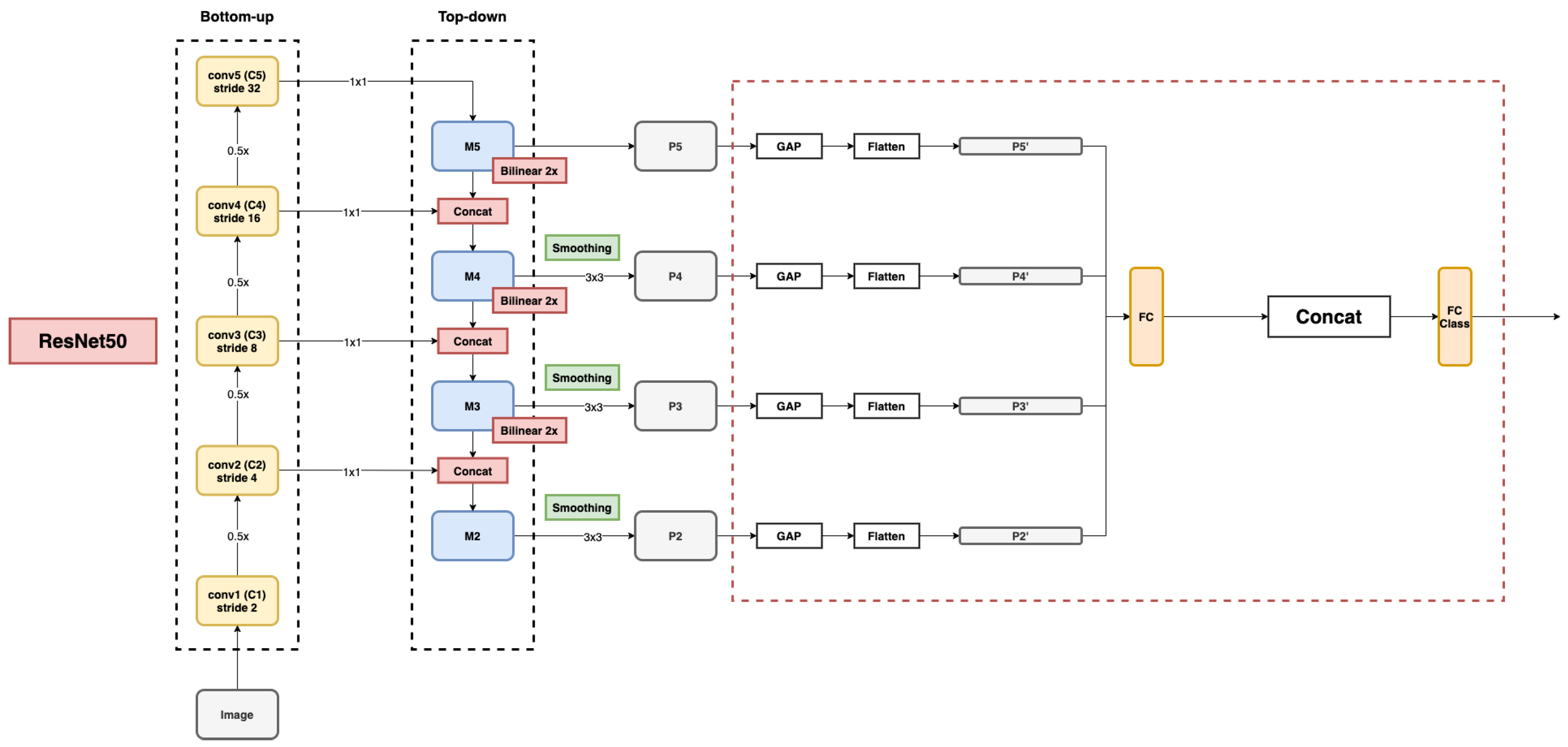
  • We train a binary CNN classifier for the task of illegal landfill detection. The proposed architecture exploits a ResNet50 backbone augmented with a Feature Pyramid Network (FPN) links [16], a technique used in object detection tasks to improve the identification of items at different scales. We evaluate the performance of the architecture on a test set of 337 images. The classifier achieves 94.5% average precision and 88.2% F1 score, with 88.6% precision at 87.7% recall. Such a result improves the accuracy w.r.t. object detection methods without requiring the manual creation of bounding boxes;
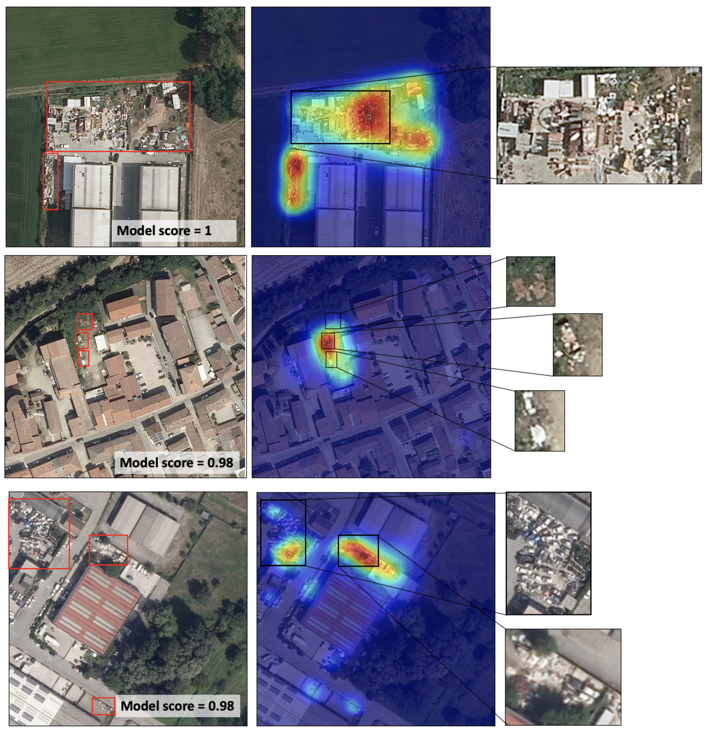
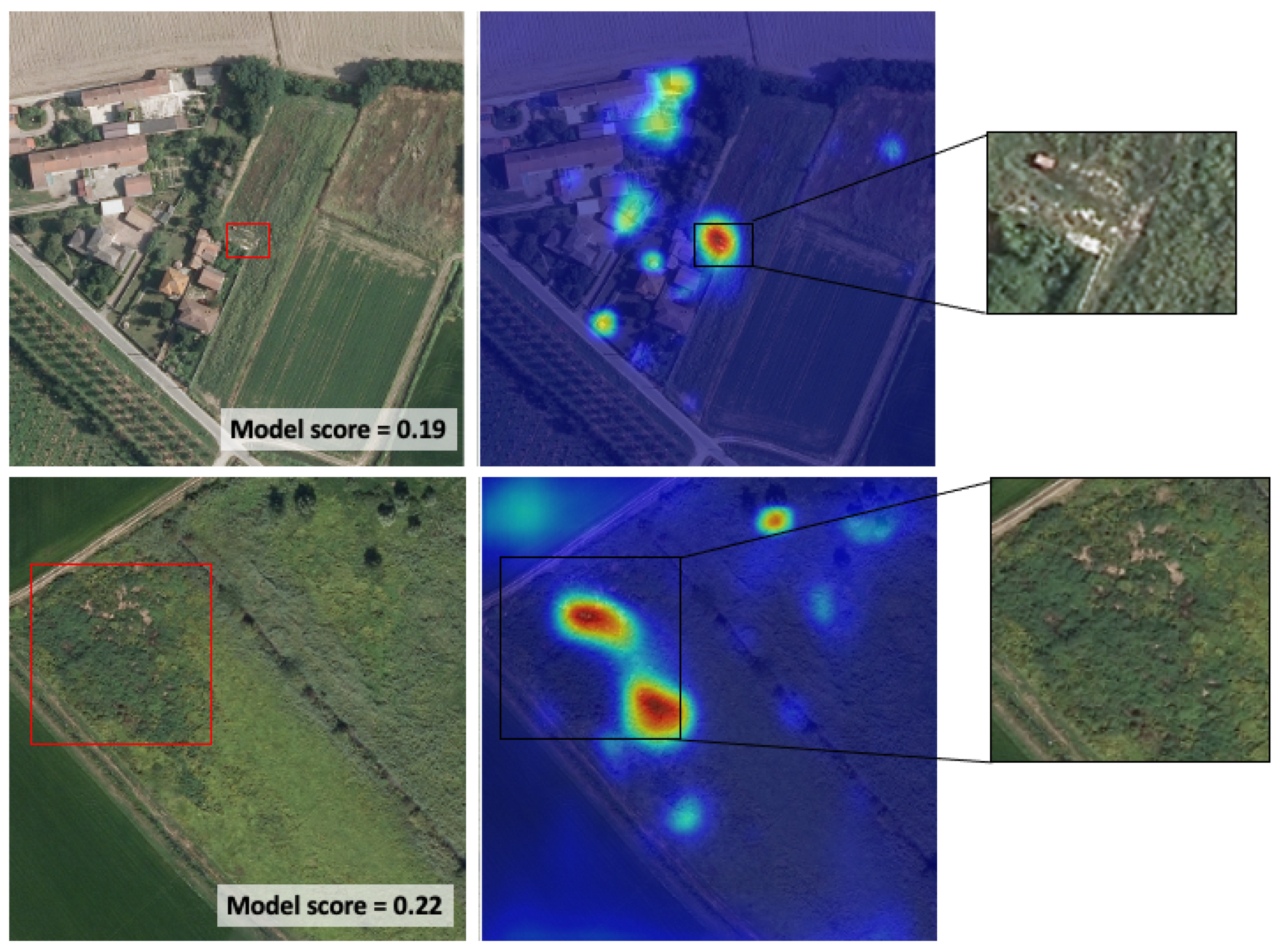
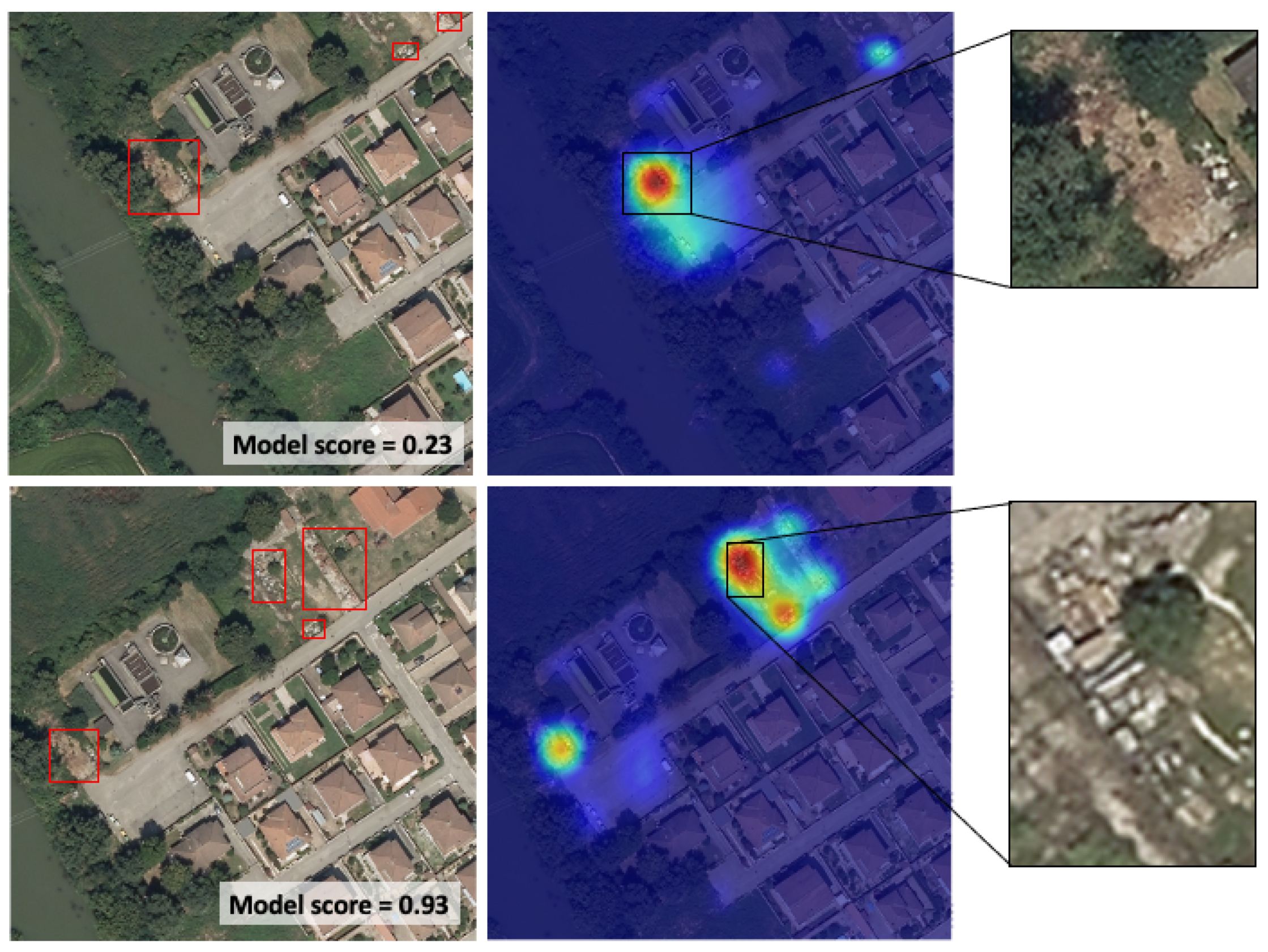
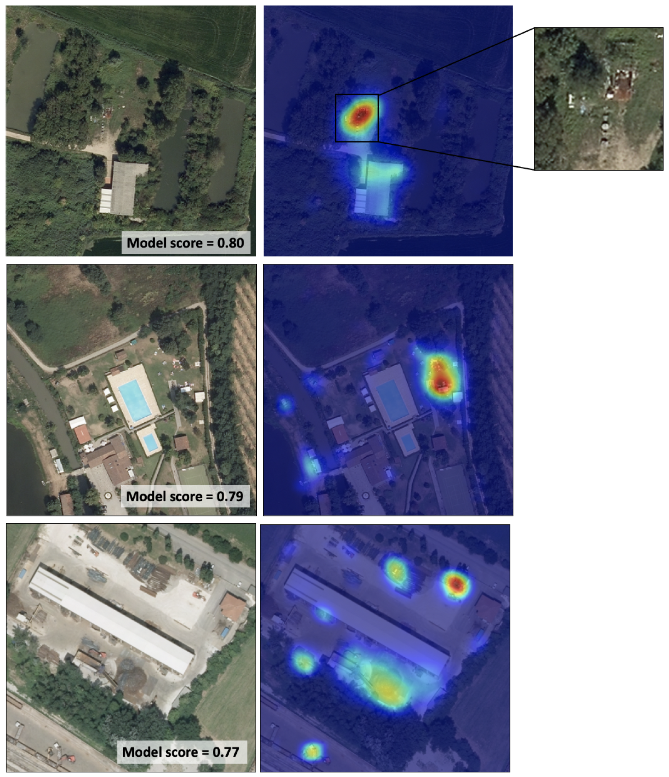
  • We analyze the output of the classifier qualitatively by exploiting visual understanding and interpretability techniques (specifically Class Attention Maps—CAMs [17]). This procedure allows identifying the representative image regions where the classifier focuses its attention.
To achieve the goals of the paper we built a dataset for the RS scene classification task in the illegal landfill domain. The dataset comprises ≈3000 images from which ≈33% are positive samples. Such positive sites were identified by experts who manually screened orthophotos at a resolution of ≈20 cm per pixel acquired during 2018 in three Italian provinces. To better situate our work in the panorama of waste detection research, we also summarize the state-of-the-art waste detection problem and organize the many heterogeneous approaches proposed in the literature by a number of characteristic dimensions.
The paper is organized as follows: Section 2 overviews the related work in the specific domain of illegal landfill identification and the more general field of deep learning applied to remote sensing scene classification, Section 3 presents the dataset used in this work, Section 4 illustrates the proposed DL approaches, Section 5 presents a quantitative and qualitative evaluation and, finally, Section 6 concludes and provides an outlook on the future work.

2. Related Work

The computer-aided identification of waste disposal sites has been an active research area for many years. The methods for identifying waste dumps can be characterized along several dimensions:
  • Data: the input data to the landfills identification process can include structured data (e.g., cadastral and administrative databases), Geographic Information System (GIS) data (e.g., land use maps, road networks), remote sensing data (optical, multi or hyperspectral), in particular, unmanned aerial vehicle (UAV) images and videos, and street-level images and videos (e.g., from surveillance cameras).
  • Time: Data can represent a snapshot at a given time or a data series acquired over a period.
  • Output: The output depends on how the problem is specified. It can be formulated as a classification task of geographic locations or of images in which an observation is labeled based on the presence or absence of illegal landfills. Alternatively, it can be defined as a CV localization task (object detection, image semantic segmentation) in which the result is a mask indicating the region of the image that belongs to the illegal landfill area. Based on these formulations, the output can be a set of positive geographical locations or images, object bounding boxes, or image segmentation masks.
  • Method: the methods can be manual, e.g., human interpretation of digital data, heuristic, or data-driven. In data-driven methods, the relevant features can be hand-crafted or learned from the data [40]. Data-driven methods in the cited works are primarily supervised and can be further distinguished based on their statistical learning approach (e.g., support vector machines (SVM), deep neural networks, CNNs).
  • Range: studies can be small range analyses focusing on the in-depth investigation of a specific landfill or small region or large scale surveys over a broad geographical area.
  • Validation: results can be validated qualitatively (e.g., by experts) or quantitatively with the aid of ground truth data (e.g., collections of images or geographic locations corresponding to known waste disposal sites).
Table 1 summarizes the characteristics of the most relevant contributions analyzed in this Section. An interesting finding is that the works using DL/CNN approaches are mainly applied to street-level imagery (6). The works applied to aerial imagery (2: [8,12]) used CNN architectures to solve an object detection task in UAV and satellite images, respectively, and produced a mask delineating the area of the image that contains waste. This analysis highlights the lack of contributions that explore alternative CNN-based methods, such as multi-scale scene detection architectures, to solve the illegal landfill problem at scale without requiring a high number of manually created bounding boxes.
Given the scarcity of directly comparable works that apply CNNs to waste dump classification, we also offer in Section 2.4 a brief overview of the results attained in DL for remote sensing scene classification in other domains.

2.1. Landfill and Waste Dump Detection from Remote Sensing Data

Early studies on waste detection using RS data focused on the human interpretation of aerial images. In 1974, the work [41] was published in which the authors proposed the use of aerial photos to determine the spatial distribution of waste producers and waste quantities. Around a decade later, the work [39] highlighted the importance of using historical aerial images to document landfills’ existence, location, extent, and possible nature. In [35], the authors studied the case of uncontrolled landfills (buried waste) in Veneto (Italy). They calculate the Stress Vegetation Index (SVI) from multispectral satellite observations. Along with an analysis of GIS information (e.g., the street network) and other historical aerial images, they find that stressed vegetation is present in all the illegal landfills and conclude that SVI is a relevant indicator. In [27], the authors classify WorldView2 high-resolution 8-band multispectral images into six categories, two of which refer to waste: building rubble and domestic dump. Overall, on a dataset of 610 observations among six categories, they obtained 85.16% accuracy on the validation split (30%) using a support vector machine. According to the authors, not all the bands have the same importance on the classification process for the different classes: the blue band is more significant for domestics dumps and the yellow one for the building rubble. They also highlight that 54% of the waste dumps occur on vacant or unused lands. In [24], the authors use images of 0.5 m spatial resolution in the panchromatic band and 2 m resolution for each multispectral band (Red, green, blue, and near InfraRed) to identify illegal landfills in the Campania region (Italy) relying on experts’ photo-interpretation. They claim that artificial intelligence (AI) cannot replace human knowledge, experience, intelligence, or understanding but acknowledge that the human eye can only interpret few layers of remotely sensed information at a time. At the same time, machine processing enables the quantitative analysis of all spectral bands simultaneously and can detect subtle differences that escape humans. As their work was performed manually, they call for the implementation of tools to make this task as automated as possible. In recent years, approaches involving DL techniques have been employed. In [12], the authors applied state-of-the-art DL models to detect landfills in satellite images. The problem is formulated as an object detection task rather than as a scene classification one. They apply the RetinaNet [15] model (with DenseNet [42] as the backbone) with a dataset with more than 2.000 images of the Shangai district annotated with bounding boxes framing the garbage. They obtained 84.7% average precision on the test set using IOU = 0.3. The authors highlight the importance of data augmentations (flip, rotation, scaling, translation) to enlarge the dataset. The authors also repeat the experiments with two image sizes (800 and 1000), obtaining different results given to the different amount of context provided. In [8], the authors also employed a multi-scale object detection approach over drone images to detect dumped waste on the riverside of Saint Lois Senegal. They annotated 5000 images with an average of 5 bounding boxes per image and trained a Single Shot Detector (SSD) model reserving 10% of the dataset for testing. The authors did not provide the characteristic metric of the object detection task (mean average precision) on the test set. From qualitative analysis, they observed that predictions vary according to the zone. The model generated many false positives given to confusion with non-waste objects (e.g., trees), and for this reason, samples from different regions will be included to continue their study.

2.2. Landfill and Waste Dump Detection from GIS and Other Structured Data

GIS information is exploited in [34], which reports a study carried out in the Veneto region divided into two areas for training and validation with 20 and 19 known illegal sites and 26 and 28 authorized ones, respectively. A weighted linear combination of different factors (presence of former quarries, proximity to authorized landfills, land use, population density) enabled the creation of a waste dump probability map. The results reported that 84.2% of the known illegal landfills were located in areas with high probability (0.67–1). Additionally, 738 new positive locations were identified as potentially relevant. In [5], the authors performed a feature analysis to determine the factors relevant to the presence of an illegal landfill and created a geo-statistical model to predict their presence. Features included the local socio-economic level, land use, proximity to urban centers, and geographic characteristics. The study was carried out in Andalusia with 518 known locations. The main finding is that the illegal landfills are not randomly distributed in the territory and 63.3% of the sites reside in areas with high predicted probability (>0.36). Similar conclusions were drawn in posterior work [31] using a logistic regression model on different features. The studies surveyed in this section use datasets provided by local administrative agencies. The number of sites in such datasets usually ranges in the order of hundreds.

2.3. Image Classification for Street-Level Visual Content

Street-level garbage detection is a problem complementary to identifying landfills in aerial images, although tackled with comparable CV methods. In [22], the authors evaluate the cleanliness of streets using a dataset of 22K geo-tagged images annotated by experts. They contrasted different feature extractors (SIFT, color histogram, CNNs based) and algorithms (Naive Bayes, SVM, among others) to classify the images into five categories (bulky item, encampment, overgrown vegetation, illegal dumping, clean). They found that training sub-models for different geographical areas yielded the best performances and reported an F1-score of 90%. In [29], the authors trained a GoogleNet [43] model with 1423 images of eight classes (tree, cart furniture, trash, trash bags, electronics, sofa, mattress). The model achieved 77% average accuracy, and the authors observed that the inclusion of the clean category introduced noise worsening performances. In [30], the authors created a dataset of 450 street-level garbage images and applied the AlexNet [44] architecture for binary classification, obtaining 87.7% average accuracy. In [23], the authors proposed a semi-supervised method for creating a segmentation mask for the garbage in the image. For the evaluation, 25 volunteers rated the segmentation masks yielding an average score of 4.1/5 for 500 images. In [45], the author analyzed 816 urban scenes and achieved an accuracy of 89% on the test set using the Faster-RCNN [46] with ResNet [47] as the backbone. In [19], the authors located the garbage in 3974 images with 5535 labels of four classes: bag, dumpster, bin, and blob (a conglomerate of objects). Using a variation of the YOLO [14] network and applying data augmentation, they achieved ≈60% mean average precision. The authors of [48] go a step further and combined object tracking and pedestrian detection to understand when someone is leaving garbage in the street from surveillance cameras. They obtained a 79% precision at 64% recall. In most of these works, state-of-the-art DL architectures were successfully applied to classify waste types at street level, showing the capability of the methods to learn features that characterize waste objects viewed up close.

2.4. Deep Learning for RS Scene Classification
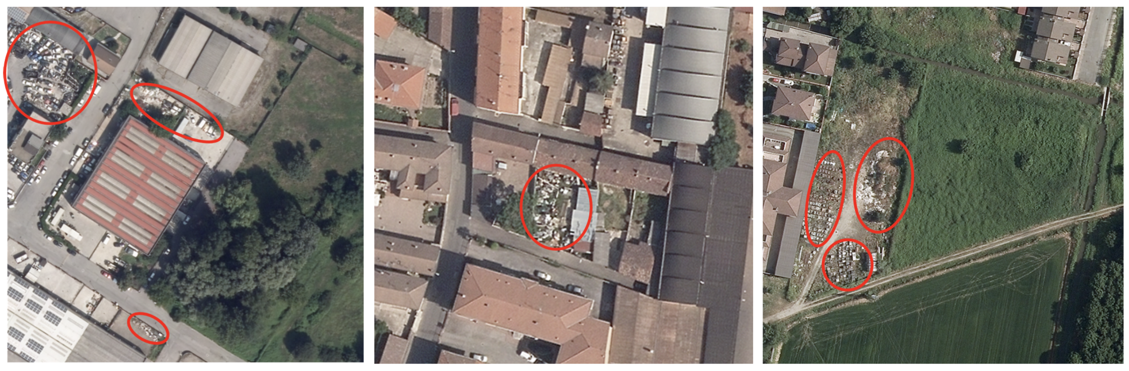
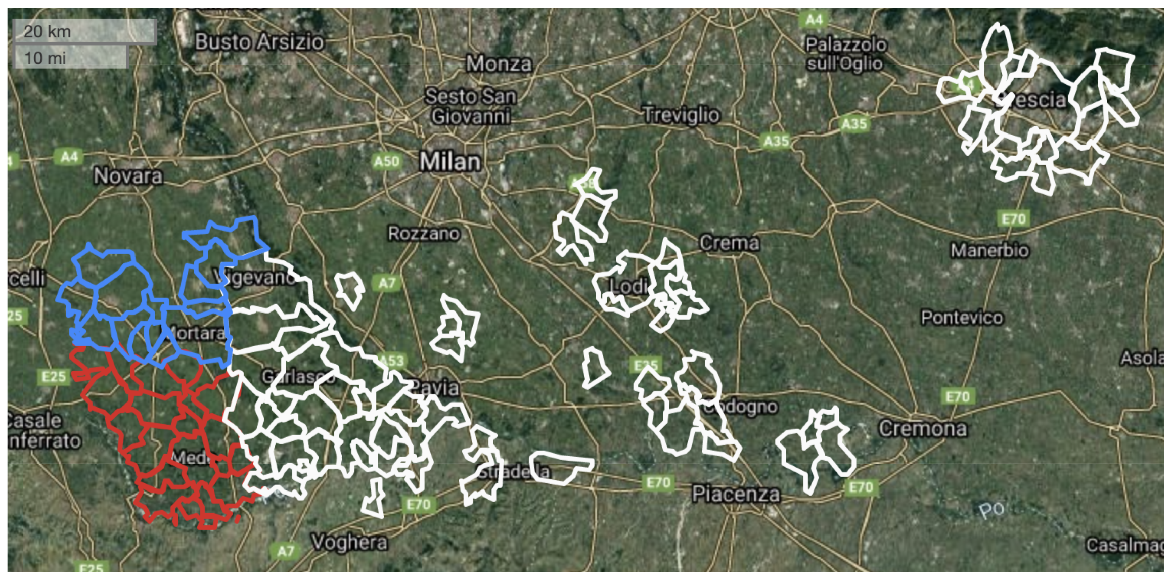
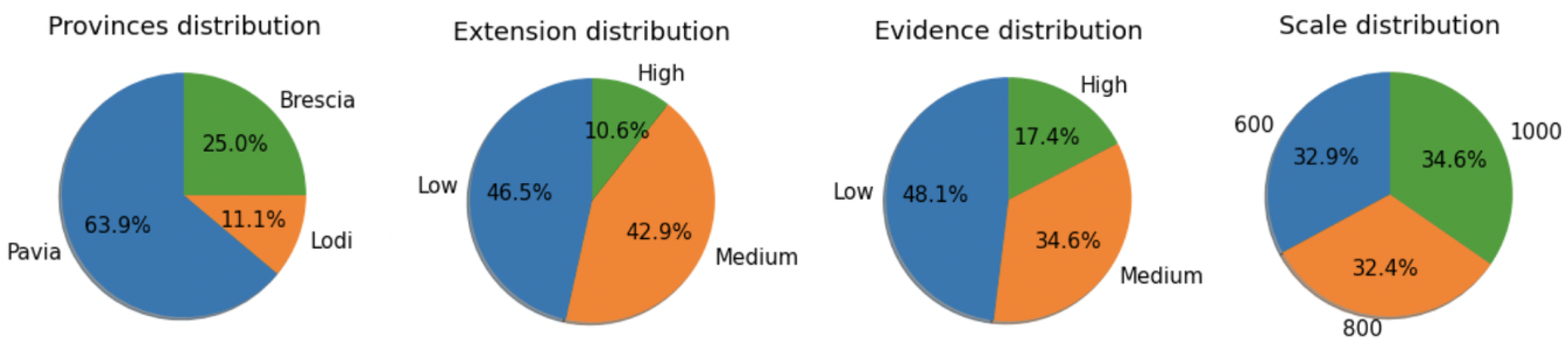
RS image classification has rapidly evolved thanks to the availability of high resolution images and to the advances in the CV field. High resolution pixels do not contain enough information to represent a whole object and pixel-wise classification does not account for the relationship between neighboring pixels. Therefore, the analysis at the object-level rather than at the pixel-level is required [49]. Furthermore, some semantic categories are characterized by multiple objects in various spatial relations (e.g., airports with planes, control towers and landing strips). The recognition of such composite configurations in aerial images is a task known as RS scene classification, which underpins our approach for detecting landfills composed of many different objects viewed from above. RS scene classification is challenging because objects may appear at different scales and with different orientations causing high intra-class diversity. Moreover, the same type of objects might compose different categories inducing high inter-class similarity.
Table 2 lists examples of RS scene classification datasets, mostly targeting land use applications. State-of-the-art datasets comprise a varying number of images per class. At one extreme, the SEN12MS dataset [50] contains classes with 31,836 images. Other datasets have much lower numbers: NWPU-RESISC45 [51] contains 700 images per class; UC-Merced [52] ≈100 images per class. Although some datasets present an unbalance in the number of images per class, other ones have the same amount of samples for all classes irrespective of the real distribution. For example, the Brazilian Coffee Scene dataset [53] contains two classes (coffee and not coffee plantations) with a very unbalanced real distribution. However, in the experiments the authors used the same amount of images for both the positive and the negative class. From the datasets listed in Table 2, one cannot conclude that there is a unique optimal number of samples for the RS scene classification task.
None of the datasets in Table 2 includes an expert-annotated landfill class. The most similar category is that of dump sites in the BigEarthNet dataset. The category is rather generic and gathers only small images with low resolution (10 m per pixel).
Early works addressing the scene classification in remote sensing focused on extracting hand-crafted features or image descriptors, such as SIFT and HOG, as inputs for supervised (e.g., SVM, RF) or unsupervised (e.g., PCA, k-means) methods. As research on CNNs emerged, different architectures were used as feature extractors. In the pioneering work [53], the CaffeNet [64] and OveraFeat [65] CNNs trained with ImageNet were used as feature extractors and compared with other 22 machine learning methods. With the UC Merced dataset, the CNNs obtained the best results (93.42% CaffeNet, 90.91% Overfeat) with a margin of ≈+17% over the best low-level descriptor method. Conversely, in the Brazilian Coffee dataset, global descriptors’ methods outperformed the CNNs by ≈+3%. This difference was motivated by the fact that UC Merced contained more complex scenes in which objects have patterns similar to those present in ImageNet, whereas in the Brazilian Coffee dataset, textures and spectral features play a dominant role. In [66], the authors proved the benefit of using the CNNs end-to-end. GoogLeNet was used to perform classification by adding a fully connected and a softmax layer achieving 97.1% accuracy with the UC Merced dataset and 91.8% with the Brazilian Coffee one.
The current research directions involve different approaches to improve classical CNNs. An example is the usage of attention methods [67,68,69] that focus the computation on the most informative parts of the input data and have improved both convergence and accuracy [70]. A different direction is that of multi-scale techniques [71,72,73] designed to cope with scenes in which objects of the same type appear with different sizes and amount of surrounding context. The idea is to combine global features with local object-level features. Another path is that of semi-supervised learning. Remote sensing offers a massive amount of imagery, but annotating these data is labor-intensive. Semi-supervised approaches help exploit unlabelled data, mainly through the use of Generative adversarial networks (GANs) [16,74].

3. Dataset

For this study, a binary dataset was used. As a starting point, the orthophotos generated by a remote sensing campaign commissioned by AGEA (https://www.agea.gov.it/, accessed on 27 September 2021 ) were acquired for the Lombardy region (Italy). The images are collected with an RGB aerophotogrammetry survey at a resolution of 20 cm per pixel. A set of 990 positive locations corresponding to sites containing waste dumps were provided to us by experts from the Environmental Protection Agency of Region of Lombardy (ARPA) from an analysis of 105 municipalities. For each site, two annotations were provided: the evidence level (low, medium, and high) specifies how confident the annotator is that a site falls under the illicit category, and the extension level (small, medium, and large) indicates the size of the site. Such annotations were not used for training but were exploited in the qualitative analysis of the results. Negative samples were randomly chosen from the territory of the same municipalities analyzed by the experts. To include unbalance into the dataset we doubled the number of negative samples with respect to the positive ones, resulting in ≈2000 negative locations. The locations were split into three geographical areas for training (75%), validation (13%), and testing (12%). Figure 2 displays the split with a color-coded representation of the sampling locations: training (white), validation (blue), and testing (red). One square image was created centered at that location for each positive and negative geographical position in the dataset. The image size was chosen randomly among three options: 600 pixels (120 m), 800 pixels (160 m), and 1000 (200 m), to include a variable amount of context in the dataset.
Figure 3 shows the distribution of the samples by province, extension level, evidence level, and image size. Most examples have low evidence or extension. At training time, data were augmented by means of a random flip (vertical and horizontal) applied to images with 25% probability.

4. Classification Approach

The binary classifier exploits ResNet50 [47] as the network backbone and augments it with a Feature Pyramid Network (FPN) architecture [75]. FPN improves performances in object detection when different scales must be taken into account [73,76] and thus can benefit also classification tasks in which objects of the same class appear with variable sizes. FPN creates a feature pyramid that has good semantics at all scales by combining low resolution semantically strong features with high resolution semantically weaker ones. This is realized by complementing the bottom up feature extraction path typical of CNNs with a top down path that builds the feature pyramid by extracting adapting and merging features at multiple levels, as shown in Figure 4. In the Figure { C 2 , C 3 , C 4 , C 5 } , respectively denote the outputs of the residual blocks of the ResNet50 stages conv2, conv3, conv4, conv5. The output of the first stage C 1 is not included in the pyramid due to its large memory footprint. The top-down path starts from C 5 and computes the merged features maps ( M 5 M 2 ), which are upsampled and de-aliased to obtain the pyramid layers { P 2 , P 3 , P 4 , P 5 } . Each P i is subjected to global average pooling (GAP) followed by a flattening operation to produce the vectors { P 2 , P 3 , P 4 , P 5 } . Each P i is input to a fully connected (FC) layer for performing classification at the respective scale level. Finally, the results of the scale-level classifiers are concatenated and used as input to the final FC layer to produce the output. The binary cross-entropy loss function is used with a learning rate of 0.005. An early stopping strategy is implemented to prevent over-fitting, with a patience factor (number of epochs with no improvement after which training will be stopped) of 10 and a min delta (minimum change in the monitored quantity to qualify as an improvement) of 0.0005.
The initialization of the ResNet50 layers is performed with transfer learning from ImageNet [77,78]. The best results were obtained by freezing the first two layers during the fine tuning. In the training phase, resizing of the input to a fixed dimension is performed to cope with images of different sizes in the same batch and to fit more images in the GPU memory. The images are also normalized based on the mean and standard deviation of the dataset. After the last FC classification layer, a Sigmoid function is added obtaining a value between 0 and 1 that denotes how confident the model is that the image belongs to the positive class [78,79]. A threshold over this value is used to classify each image. The model was trained using two Nvidia GeForce RTX 2080Ti GPUs. The batch size was set to 12 (given the capacity of the server). The weights of the trained model, as well as additional details on the training phase are published on GitHub (https://github.com/rnt-pmi/remote-sensing-scene-classification-landfills, accessed on 27 September 2021).

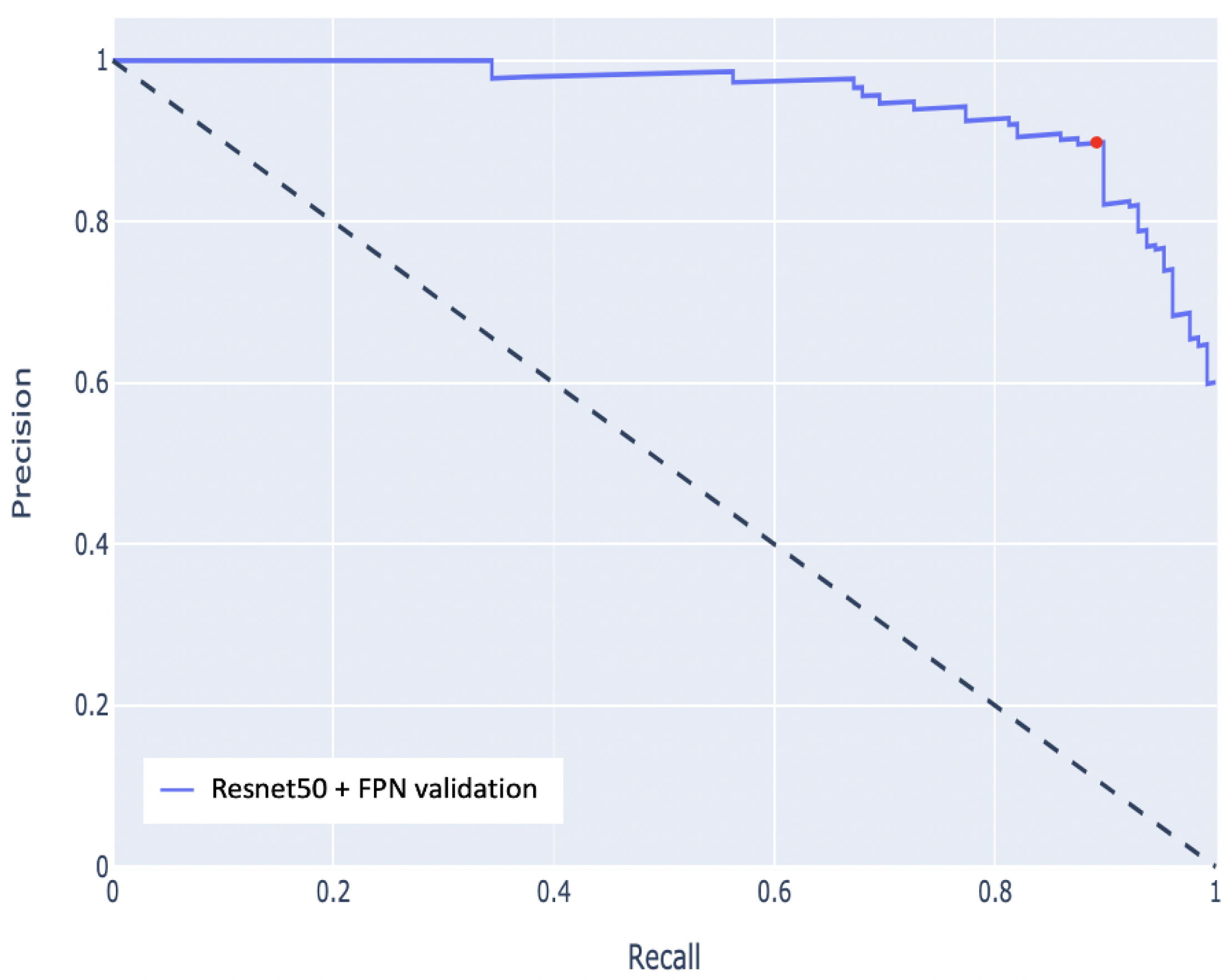
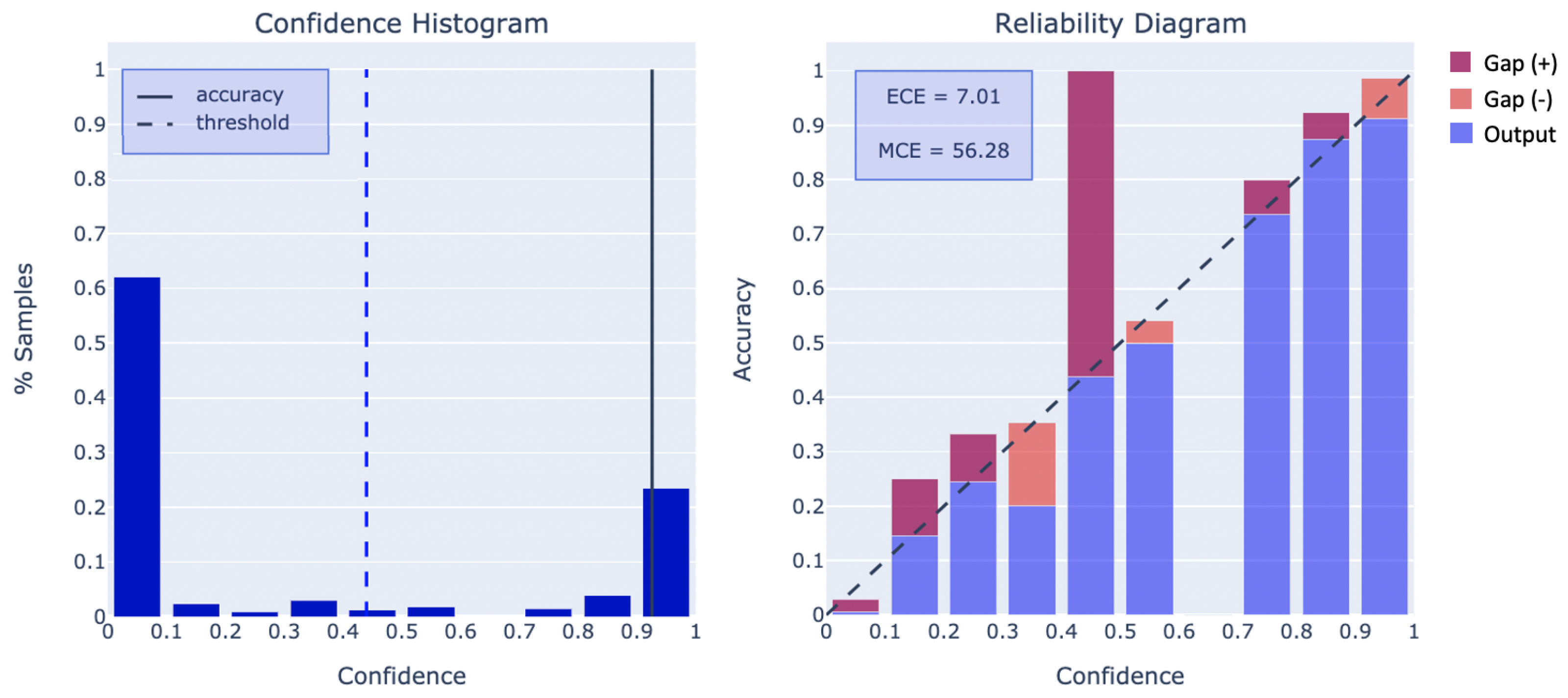
5. Quantitative Analysis

The binary classification of input samples is performed by setting a threshold on the confidence score produced as output by the ResNet50 + FPN model. Figure 5 shows the precision and recall (PR) curve computed on the validation dataset by varying the threshold [80]. The value to use for the test dataset ( 0.44 ) is chosen as the one that maximises the F1 score on the validation dataset. Maximising F1 makes a good compromise between the number of missed positive samples and the number of irrelevant sites reported as positives, which would cause unnecessary interpretation work for the analyst. Table 3 presents the results of applying the classifier to the test dataset. The evaluated metrics comprise the average precision (AP), which summarizes the PR curve as the weighted mean of precision values achieved at each threshold, accuracy, precision, recall, F1-score, and ECE (described next). A moderate drop in performances is observed when switching from the validation to the test dataset ( 1.2 in F1-score). However, the model generalizes very well on the test dataset with AP exceeding 94% and ≈90% precision at ≈89% recall.
The expected calibration error (ECE) indicates how well the probability estimates can be interpreted as correctness likelihood. In a well-calibrated classifier of all the samples that are predicted with a probability estimate of, say, 0.6 (around 60%), should belong to the positive class [81]. Calibration is related to the reliability of the confidence score, which is a critical property when a classification model is exploited to make predictions for high-risk or sensitive applications. In the case of illegal landfills detection, it is particularly important that the model output reflects the actual underlying probability of the positive class to support the decision of inspecting a suspicious site. Figure 6 shows the confidence distribution diagram and the reliability diagram [81] of our ResNet50 + FPN model. The confidence distribution diagram shows that the model assigns a low confidence value to nearly twice as many as the samples it rates with high confidence. This proportion reflects the class distribution in the dataset since there are nearly twice as many negative samples as there are positive ones. The reliability diagram contrasts the model behavior with the ideal case represented by the diagonal line, which denotes a perfectly calibrated model. Figure 6 also reports the expected calibration error (ECE) (Equation (1)) and maximum calibration error (MCE) (Equation (2)) defined as follows:
E C E = m = 1 M B m n a c c ( B m ) c o n f ( B m )
M C E = m a x m ϵ ( 1 . . M ) | a c c ( B m ) c o n f ( B m ) |
where n is the number of samples in the dataset, M is the number of buckets (each of size 1/M), and B m denotes the set of indices of observations whose prediction confidence falls into the interval m.
As shown in Figure 6, in most cases, the model is moderately more confident than it should be, except in the 0.4–0.5 bucket, where the over-confidence is high, giving an MCE of 56. Such a bin has a small effect on the ECE (7.01) given the low number of samples in this range, as visible in the confidence distribution histogram. An ECE of 7.01 shows that the model is well-calibrated, and thus, the analyst could use its estimates as realistic proxies of the actual probabilities.

6. Qualitative Analysis

A visual inspection of the results helps understand the behavior of the model. The classification of illegal landfill scenes relies on the presence of diverse objects, such as dumpsters, scattered debris, tires, containers, and others. Thus it is interesting to examine which objects are responsible for predicting a site as a waste dump. To this end, the computation of Class Activation Maps (CAMs) [17] can be used to highlight the regions of the input image with the greatest influence on the model prediction. A CAM is a matrix that is scaled to the same dimensions as the input image and associated with a specific output class. Each CAM cell contains a value denoting the relevance of the pixel with respect to the class of interest. Visually, CAMs can overlay a heat map representation onto the input image to highlight the pixels with the higher relevance for a specific class. In our multi-scale context, CAMs are computed at every scale level and multiplied by the weights of that scale in the last FC layer. Finally, they are combined by element-wise addition and normalized in the 0 to 1 range. Figure 7, Figure 8, Figure 9 and Figure 10 exemplify input images overlaid with the heat maps derived from the respective CAMs.

6.1. Examples of True Positives

Figure 7 exemplifies sites classified correctly and with high confidence (≥98%). Red boxes are provided to highlight the objects that led the analyst to classify the image as a positive one. The first example shows a production plant with a waste storage area and various materials (messy and often very large). The waste dumps regions have a well-delimited boundary and cover a large part of the image. The model focuses on them quite precisely, as shown by the CAM heat maps. In the second example, the significant objects are concentrated in a much smaller part of the image, nonetheless appear as relevant in the CAM heat map. As suggested by these two examples, the multi-scale analysis capability afforded by the FPN links helps the detection of relevant objects of different sizes and coverage. In the third example, the attention focuses on a group of abandoned cars, which highlights the capability of the classifier to cope with the intra-class diversity challenge typical of the waste detection task, in which objects of very different nature may contribute to the prediction.
The three examples demonstrate the recognition of disparate types of objects with different sizes and distributions within the image. The model is able to classify all of them with very high confidence tackling the intra-class dissimilarity and multi-scale challenges adequately.

6.2. Examples of False Negatives

Figure 8 illustrates two cases that were incorrectly classified as negative even if the expert interpreter had labeled them as containing waste dumps.
The first image shows a site where some waste is visible close to the north wall of a property and inside the courtyard. In this scene, the CAM components are small and sparse and overlay regions with rather generic visual content. More intensity can be seen in the rightmost CAM component, but this is still insufficient to obtain a high classification score for the whole image. The second case is a site where the presence of waste is only perceivable indirectly. The experienced photo interpreter noted a patch of stressed vegetation, which could be a clue of liquid or buried waste. The model fails to classify the site correctly only from such weak clues. A multi-spectral analysis and the computation of the vegetation stress index could help solve this case as well [35].
Figure 9 shows a case of wrong negative classification due to the lack of significant context in the image. The first image shows the original sample from the dataset, which was classified as negative. However, a small shift of the focus to the north-east reveals a missing part of the scene, which unveils an access road and a field full of litter. When the whole context is provided, the model achieves high confidence and correctly classifies the scene. The occurrence of wrong classifications caused by the fragmentation of a significant scene across multiple input samples can be mitigated by increasing the overlap between the images of the testing set, to the price of an increase in the computational cost.
In most false negative cases, the CAMs show that the most relevant areas for the model usually coincide with those highlighted by the human expert. However, the contribution of such areas to the activation is not enough to trigger the classification layer. The average confidence of the model for the false negatives is ≈0.17 and most false positives in the test set were characterized by the expert with “low” (46%) and “medium” (40%) extension and “low” (35%) and “medium” (35%) evidence.

6.3. False Positive Analysis

Figure 10 presents three cases classified as positive by the model and not considered as such by the human expert. The first image represents a scene where some scattered objects are visible close to a large shed served by a secondary road. The general configuration looks similar to that of the typical waste dump, but the photo interpreter judged that the visible objects were not sufficiently clear to justify a positive assessment. The second example illustrates well the challenge of inter-class similarity. It consists of a swimming pool area with sun umbrellas and deckchairs. Such objects could be confused with plastic bags, usually present in waste dumping sites. Although for the human eye it is easy to infer the real nature of the site based on the context, the model is unable to make the distinction. In the third example, the model classifies positively a plant that collects metal scraps. The CAM heat map shows that the model focuses on a big heap of metal scraps and an area piled with tubes. However, the photo interpreter used other information (the location address and the yellow page directory) to exclude the site from the suspicious ones.
In most false positive cases, the analyst excluded the danger of a site by visual inspection or by resorting to collateral information not available to the image classifier. The average confidence of the model for the false positives is ≈0.7 (70%). This value could be used to prioritize the positively classified locations, selecting for human validation suspicious sites with confidence ≥70% first.

7. Conclusions and Future Work

In this paper, we have addressed the detection of illegal landfills with a binary remote sensing scene classification task. A dataset was created with the help of experts using remote sensing imagery. The classical ResNet50 CNN was combined with components of the FPN architecture to improve the extraction of features at different scales to classify better images containing relevant objects of different sizes and extensions. The resulting architecture was trained and evaluated. The classifier achieves 94.5% average precision and 88.2% F1 score, with 88.6% precision at 87.7% recall. The qualitative analysis conducted with the support of Class Activation Maps (CAMs) provided further insight. In particular, improvements can be obtained by increasing the overlap between images extracted from the survey data and by considering non-visual information to enrich the classifier’s input. The qualitative analysis with CAMs also proved that the model tends to focus on the same aspects considered by the human expert. This information can be provided to the analyst as a guide on where to look, which can accelerate the photo interpretation process.
Future work will concentrate on new tasks and research directions:
  • Dataset extension. As analysts inspect new territories, their findings will be incorporated into the dataset, improving the model. Specifically, complex negative examples will be sought. In the present work, negative examples were sampled randomly, but choosing them based on semantic information (e.g., vicinity to “difficult” contexts, such as swimming pools and cemeteries) could reduce false positives substantially;
  • Different imagery. The described analysis was executed on a single type of image with a resolution of 20 cm per pixel. The experimentation with other resolutions and different remote sensing products beyond the visible band could lead to more accurate classification, e.g., including the NIR band to exploit the presence of stressed vegetation as a clue for buried waste;
  • Classification of waste types. The type of waste present at a location is a clue that helps the analyst categorize a site. Examples include plastic, tires, grouped cars, bulky waste, sludge, or manure. Moreover, waste treatment plants might intentionally misclassify waste to deceive law enforcement authorities, e.g., by using non-hazardous waste codes for hazardous materials. In this scenario, classifying images based on the type of waste is extremely useful;
  • Weakly supervised segmentation. Understanding the extension of relevant objects could help estimate the level of risk associated with a detected site, which would help prioritize interventions. Object detection and instance segmentation tools output bounding boxes and masks from which the area of a waste dump can be computed. However, training an object detection or instance segmentation model requires a costly and time-consuming ground truth production process. Weakly supervised methods have attracted interest in recent years to reduce the effort of ground truth creation. Illegal landfill detection could be a perfect use case to apply state-of-the-art weakly-supervised approaches;
  • Multi-temporal analysis. Analyzing images taken at different dates could provide information on the site activity, e.g., growing or shrinking;
  • Model efficiency. The ultimate goal of automating the photo interpretation task is enabling the complete scanning of the territory at a vast scale in a limited amount of time or even the implementation of near real-time alerting of the insurgence of waste-related risks. This objective requires a substantial reduction in the inference time coupled with a limited loss in prediction reliability.

Author Contributions

Conceptualization, R.N.T. and P.F.; methodology, R.N.T. and P.F.; software, R.N.T.; validation, R.N.T. and P.F.; formal analysis, R.N.T. and P.F.; investigation, R.N.T. and P.F.; writing—original draft preparation, R.N.T. and P.F.; writing—review and editing, R.N.T. and P.F.; visualization, R.N.T.; supervision, R.N.T. and P.F. All authors have read and agreed to the published version of the manuscript.

Funding

This research received no external funding.

Institutional Review Board Statement

Not applicable.

Informed Consent Statement

Not applicable.

Data Availability Statement

The data are not publicly available due to the sensitive information on locations that are under investigation and law enforcement.

Acknowledgments

We wish to thank the Environmental Protection Agency of Region of Lombardy (ARPA Lombardia) for the collaboration in the acquisition of the imagery and in the construction of the ground truth employed in this study.

Conflicts of Interest

The authors declare no conflict of interest.

References

  1. Association, E.S. Rethinking Waste Crime. 2017. Available online: http://www.esauk.org/application/files/7515/3589/6448/20170502_Rethinking_Waste_Crime.pdf (accessed on 25 May 2021).
  2. Rocco, G.; Petitti, T.; Martucci, N.; Piccirillo, M.C.; La Rocca, A.; La Manna, C.; De Luca, G.; Morabito, A.; Chirico, A.; Franco, R.; et al. Survival after surgical treatment of lung cancer arising in the population exposed to illegal dumping of toxic waste in the land of fires (‘Terra dei Fuochi’) of Southern Italy. Anticancer Res. 2016, 36, 2119–2124. [Google Scholar]
  3. Schrab, G.E.; Brown, K.W.; Donnelly, K. Acute and genetic toxicity of municipal landfill leachate. Water Air Soil Pollut. 1993, 69, 99–112. [Google Scholar] [CrossRef] [Green Version]
  4. Limoli, A.; Garzia, E.; De Pretto, A.; De Muri, C. Illegal landfill in Italy (EU)—A multidisciplinary approach. Environ. Forensics 2019, 20, 26–38. [Google Scholar] [CrossRef]
  5. Jordá-Borrell, R.; Ruiz-Rodríguez, F.; Lucendo-Monedero, Á.L. Factor analysis and geographic information system for determining probability areas of presence of illegal landfills. Ecol. Indic. 2014, 37, 151–160. [Google Scholar] [CrossRef]
  6. Quesada-Ruiz, L.C.; Rodriguez-Galiano, V.; Jordá-Borrell, R. Characterization and mapping of illegal landfill potential occurrence in the Canary Islands. Waste Manag. 2019, 85, 506–518. [Google Scholar] [CrossRef]
  7. Slonecker, T.; Fisher, G.B.; Aiello, D.P.; Haack, B. Visible and infrared remote imaging of hazardous waste: A review. Remote Sens. 2010, 2, 2474–2508. [Google Scholar] [CrossRef] [Green Version]
  8. Youme, O.; Bayet, T.; Dembele, J.M.; Cambier, C. Deep Learning and Remote Sensing: Detection of Dumping Waste Using UAV. Procedia Comput. Sci. 2021, 185, 361–369. [Google Scholar] [CrossRef]
  9. Wurm, M.; Stark, T.; Zhu, X.X.; Weigand, M.; Taubenböck, H. Semantic segmentation of slums in satellite images using transfer learning on fully convolutional neural networks. ISPRS J. Photogramm. Remote Sens. 2019, 150, 59–69. [Google Scholar] [CrossRef]
  10. Helber, P.; Bischke, B.; Dengel, A.; Borth, D. Eurosat: A novel dataset and deep learning benchmark for land use and land cover classification. IEEE J. Sel. Top. Appl. Earth Obs. Remote Sens. 2019, 12, 2217–2226. [Google Scholar] [CrossRef] [Green Version]
  11. Zhang, L.; Zhang, L.; Du, B. Deep learning for remote sensing data: A technical tutorial on the state of the art. IEEE Geosci. Remote Sens. Mag. 2016, 4, 22–40. [Google Scholar] [CrossRef]
  12. Abdukhamet, S. Landfill Detection in Satellite Images Using Deep Learning. Master’s Thesis, Shanghai Jiao Tong University, Shanghai, China, 2019. [Google Scholar]
  13. Cheng, G.; Xie, X.; Han, J.; Guo, L.; Xia, G.S. Remote Sensing Image Scene Classification Meets Deep Learning: Challenges, Methods, Benchmarks, and Opportunities. arXiv 2020, arXiv:2005.01094. [Google Scholar] [CrossRef]
  14. Redmon, J.; Divvala, S.; Girshick, R.; Farhadi, A. You only look once: Unified, real-time object detection. In Proceedings of the IEEE Conference on Computer Vision and Pattern Recognition, Las Vegas, NV, USA, 27–30 June 2016; pp. 779–788. [Google Scholar]
  15. Lin, T.Y.; Goyal, P.; Girshick, R.; He, K.; Dollár, P. Focal loss for dense object detection. In Proceedings of the IEEE International Conference on Computer Vision, Venice, Italy, 22–29 October 2017; pp. 2980–2988. [Google Scholar]
  16. Lin, D.; Fu, K.; Wang, Y.; Xu, G.; Sun, X. MARTA GANs: Unsupervised representation learning for remote sensing image classification. IEEE Geosci. Remote Sens. Lett. 2017, 14, 2092–2096. [Google Scholar] [CrossRef] [Green Version]
  17. Zhou, B.; Khosla, A.; Lapedriza, A.; Oliva, A.; Torralba, A. Learning deep features for discriminative localization. In Proceedings of the IEEE Conference on Computer Vision and Pattern Recognition, Las Vegas, NV, USA, 27–30 June 2016; pp. 2921–2929. [Google Scholar]
  18. Kazaryan, M.; Simonyan, A.; Simavoryan, S.; Ulitina, E.; Aramyan, R. Waste disposal facilities monitoring based on high-resolution information features of space images. E3S Web Conf. 2020, 157, 02029. [Google Scholar] [CrossRef] [Green Version]
  19. De Carolis, B.; Ladogana, F.; Macchiarulo, N. YOLO TrashNet: Garbage Detection in Video Streams. In Proceedings of the 2020 IEEE Conference on Evolving and Adaptive Intelligent Systems (EAIS), Bari, Italy, 27–29 May 2020; pp. 1–7. [Google Scholar]
  20. Gill, J.; Faisal, K.; Shaker, A.; Yan, W.Y. Detection of waste dumping locations in landfill using multi-temporal Landsat thermal images. Waste Manag. Res. 2019, 37, 386–393. [Google Scholar] [CrossRef] [Green Version]
  21. Jakiel, M.; Bernatek-Jakiel, A.; Gajda, A.; Filiks, M.; Pufelska, M. Spatial and temporal distribution of illegal dumping sites in the nature protected area: The Ojców National Park, Poland. J. Environ. Plan. Manag. 2019, 62, 286–305. [Google Scholar] [CrossRef]
  22. Alfarrarjeh, A.; Kim, S.H.; Agrawal, S.; Ashok, M.; Kim, S.Y.; Shahabi, C. Image classification to determine the level of street cleanliness: A case study. In Proceedings of the IEEE Fourth International Conference on Multimedia Big Data (BigMM), Xi’an, China, 13–18 September 2018; pp. 1–5. [Google Scholar]
  23. Anjum, M.; Umar, M.S. Garbage localization based on weakly supervised learning in Deep Convolutional Neural Network. In Proceedings of the 2018 International Conference on Advances in Computing, Communication Control and Networking (ICACCCN), Greater Noida, India, 12–13 October 2018; pp. 1108–1113. [Google Scholar]
  24. Angelino, C.; Focareta, M.; Parrilli, S.; Cicala, L.; Piacquadio, G.; Meoli, G.; De Mizio, M. A case study on the detection of illegal dumps with GIS and remote sensing images. In Earth Resources and Environmental Remote Sensing/GIS Applications IX; International Society for Optics and Photonics: Bellingham, WA, USA, 2018; Volume 10790, p. 107900M. [Google Scholar]
  25. Rad, M.S.; von Kaenel, A.; Droux, A.; Tieche, F.; Ouerhani, N.; Ekenel, H.K.; Thiran, J.P. A computer vision system to localize and classify wastes on the streets. In Proceedings of the International Conference on Computer Vision Systems, Las Vegas, NV, USA, 27–30 June 2017; pp. 195–204. [Google Scholar]
  26. Manzo, C.; Mei, A.; Zampetti, E.; Bassani, C.; Paciucci, L.; Manetti, P. Top-down approach from satellite to terrestrial rover application for environmental monitoring of landfills. Sci. Total Environ. 2017, 584, 1333–1348. [Google Scholar] [CrossRef]
  27. Selani, L. Mapping Illegal Dumping Using a High Resolution Remote Sensing Image Case Study: Soweto Township in South Africa. Ph.D. Thesis, University of the Witwatersrand, Johannesburg, South Africa, 2017. [Google Scholar]
  28. Begur, H.; Dhawade, M.; Gaur, N.; Dureja, P.; Gao, J.; Mahmoud, M.; Huang, J.; Chen, S.; Ding, X. An edge-based smart mobile service system for illegal dumping detection and monitoring in San Jose. In Proceedings of the 2017 IEEE SmartWorld, Ubiquitous Intelligence & Computing, Advanced & Trusted Computed, Scalable Computing & Communications, Cloud & Big Data Computing, Internet of People and Smart City Innovation (SmartWorld/SCALCOM/UIC/ATC/CBDCom/IOP/SCI), San Francisco, CA, USA, 4–8 August 2017; pp. 1–6. [Google Scholar]
  29. Dabholkar, A.; Muthiyan, B.; Srinivasan, S.; Ravi, S.; Jeon, H.; Gao, J. Smart illegal dumping detection. In Proceedings of the 2017 IEEE Third International Conference on Big Data Computing Service and Applications (BigDataService), San Francisco, CA, USA, 6–9 April 2017; pp. 255–260. [Google Scholar]
  30. Mittal, G.; Yagnik, K.B.; Garg, M.; Krishnan, N.C. Spotgarbage: Smartphone app to detect garbage using deep learning. In Proceedings of the 2016 ACM International Joint Conference on Pervasive and Ubiquitous Computing, Heidelberg, Germany, 12–16 September 2016; pp. 940–945. [Google Scholar]
  31. Lucendo-Monedero, A.L.; Jordá-Borrell, R.; Ruiz-Rodríguez, F. Predictive model for areas with illegal landfills using logistic regression. J. Environ. Plan. Manag. 2015, 58, 1309–1326. [Google Scholar] [CrossRef]
  32. Viezzoli, A.; Edsen, A.; Auken, E.; Silvestri, S. The Use of Satellite Remote Sensing and Helicopter Tem Data for the Identification and Characterization of Contaminated. In Proceedings of the Near Surface 2009-15th EAGE European Meeting of Environmental and Engineering Geophysics. European Association of Geoscientists & Engineers, Dublin, Ireland, 17–19 September 2009; p. cp–134. [Google Scholar]
  33. Chinatsu, Y. Possibility of monitoring of waste disposal site using satellite imagery. JIFS 2009, 6, 23–28. [Google Scholar]
  34. Biotto, G.; Silvestri, S.; Gobbo, L.; Furlan, E.; Valenti, S.; Rosselli, R. GIS, multi-criteria and multi-factor spatial analysis for the probability assessment of the existence of illegal landfills. Int. J. Geogr. Inf. Sci. 2009, 23, 1233–1244. [Google Scholar] [CrossRef]
  35. Silvestri, S.; Omri, M. A method for the remote sensing identification of uncontrolled landfills: Formulation and validation. Int. J. Remote Sens. 2008, 29, 975–989. [Google Scholar] [CrossRef]
  36. Notarnicola, C.; Angiulli, M.; Giasi, C.I. Southern Italy illegal dumps detection based on spectral analysis of remotely sensed data and land-cover maps. In Remote Sensing for Environmental Monitoring, GIS Applications, and Geology III; International Society for Optics and Photonics: Bellingham, WA, USA, 2004; Volume 5239, pp. 483–493. [Google Scholar]
  37. Salleh, J.B.; Tsudagawa, M. Classification of industrial disposal illegal dumping site images by using spatial and spectral information together. In Proceedings of the 19th IEEE Instrumentation and Measurement Technology Conference (IEEE Cat. No. 00CH37276), IMTC/200, Anchorage, AK, USA, 21–23 May 2002; Volume 1, pp. 559–563. [Google Scholar]
  38. Lyon, J. Use of maps, aerial photographs, and other remote sensor data for practical evaluations of hazardous waste sites. Photogramm. Eng. Remote Sens. 1987, 53, 515–519. [Google Scholar]
  39. Erb, T.L.; Philipson, W.R.; Teng, W.L.; Liang, T. Analysis of landfills with historic airphotos. Photogramm. Eng. Remote Sens. 1981, 47, 1363–1369. [Google Scholar]
  40. Nanni, L.; Ghidoni, S.; Brahnam, S. Handcrafted vs. non-handcrafted features for computer vision classification. Pattern Recognit. 2017, 71, 158–172. [Google Scholar] [CrossRef]
  41. Garofalo, D.; Wobber, F. Solid waste and remote sensing. Photogramm. Eng. 1974, 40, 45–59. [Google Scholar]
  42. Huang, G.; Liu, Z.; Van Der Maaten, L.; Weinberger, K.Q. Densely connected convolutional networks. In Proceedings of the IEEE Conference on Computer Vision and Pattern Recognition, Honolulu, HI, USA, 21–27 July 2017; pp. 4700–4708. [Google Scholar]
  43. Szegedy, C.; Liu, W.; Jia, Y.; Sermanet, P.; Reed, S.; Anguelov, D.; Erhan, D.; Vanhoucke, V.; Rabinovich, A. Going deeper with convolutions. In Proceedings of the IEEE Conference on Computer Vision and Pattern Recognition, Boston, MA, USA, 7–15 June 2015; pp. 1–9. [Google Scholar]
  44. Krizhevsky, A.; Sutskever, I.; Hinton, G.E. Imagenet classification with deep convolutional neural networks. Adv. Neural Inf. Process. Syst. 2012, 25, 1097–1105. [Google Scholar] [CrossRef]
  45. Wang, Y.; Zhang, X. Autonomous garbage detection for intelligent urban management. In Proceedings of the MATEC Web of Conferences. EDP Sciences, Shanghai, China, 12–14 October 2018; Volume 232, p. 01056. [Google Scholar]
  46. Girshick, R. Fast r-cnn. In Proceedings of the IEEE International Conference on Computer Vision, Santiago, Chile, 7–13 December 2015; pp. 1440–1448. [Google Scholar]
  47. He, K.; Zhang, X.; Ren, S.; Sun, J. Deep residual learning for image recognition. In Proceedings of the IEEE Conference on Computer Vision and Pattern Recognition, Las Vegas, NV, USA, 27–30 June 2016; pp. 770–778. [Google Scholar]
  48. Yun, K.; Kwon, Y.; Oh, S.; Moon, J.; Park, J. Vision-based garbage dumping action detection for real-world surveillance platform. ETRI J. 2019, 41, 494–505. [Google Scholar] [CrossRef]
  49. Blaschke, T.; Strobl, J. What’s wrong with pixels? Some recent developments interfacing remote sensing and GIS. Z. Geoinformationssysteme 2001, 14, 12–17. [Google Scholar]
  50. Schmitt, M.; Wu, Y.L. Remote Sensing Image Classification with the SEN12MS Dataset. arXiv 2021, arXiv:2104.00704. [Google Scholar]
  51. Cheng, G.; Han, J.; Lu, X. Remote sensing image scene classification: Benchmark and state of the art. Proc. IEEE 2017, 105, 1865–1883. [Google Scholar] [CrossRef] [Green Version]
  52. Yang, Y.; Newsam, S. Bag-of-visual-words and spatial extensions for land-use classification. In Proceedings of the 18th SIGSPATIAL International Conference on Advances in Geographic Information Systems, San Jose, CA, USA, 2–5 November 2010; pp. 270–279. [Google Scholar]
  53. Penatti, O.A.; Nogueira, K.; Dos Santos, J.A. Do deep features generalize from everyday objects to remote sensing and aerial scenes domains? In Proceedings of the 2015 IEEE Conference on Computer Vision and Pattern Recognition Workshops (CVPRW), Boston, MA, USA, 7–15 June 2015; pp. 44–51. [Google Scholar]
  54. Zhao, B.; Zhong, Y.; Xia, G.S.; Zhang, L. Dirichlet-derived multiple topic scene classification model for high spatial resolution remote sensing imagery. IEEE Trans. Geosci. Remote Sens. 2015, 54, 2108–2123. [Google Scholar] [CrossRef]
  55. Zou, Q.; Ni, L.; Zhang, T.; Wang, Q. Deep learning based feature selection for remote sensing scene classification. IEEE Geosci. Remote Sens. Lett. 2015, 12, 2321–2325. [Google Scholar] [CrossRef]
  56. Zhao, L.; Tang, P.; Huo, L. Feature significance-based multibag-of-visual-words model for remote sensing image scene classification. J. Appl. Remote Sens. 2016, 10, 035004. [Google Scholar] [CrossRef]
  57. Xu, S.; Fang, T.; Li, D.; Wang, S. Object classification of aerial images with bag-of-visual words. IEEE Geosci. Remote Sens. Lett. 2009, 7, 366–370. [Google Scholar]
  58. Xia, G.S.; Hu, J.; Hu, F.; Shi, B.; Bai, X.; Zhong, Y.; Zhang, L.; Lu, X. AID: A benchmark data set for performance evaluation of aerial scene classification. IEEE Trans. Geosci. Remote Sens. 2017, 55, 3965–3981. [Google Scholar] [CrossRef] [Green Version]
  59. Li, H.; Dou, X.; Tao, C.; Hou, Z.; Chen, J.; Peng, J.; Deng, M.; Zhao, L. RSI-CB: A large scale remote sensing image classification benchmark via crowdsource data. Sensors 2020, 20, 1594. [Google Scholar] [CrossRef] [Green Version]
  60. Wang, Q.; Liu, S.; Chanussot, J.; Li, X. Scene classification with recurrent attention of VHR remote sensing images. IEEE Trans. Geosci. Remote Sens. 2018, 57, 1155–1167. [Google Scholar] [CrossRef]
  61. Sumbul, G.; Charfuelan, M.; Demir, B.; Markl, V. Bigearthnet: A large-scale benchmark archive for remote sensing image understanding. In Proceedings of the IGARSS 2019-2019 IEEE International Geoscience and Remote Sensing Symposium, Yokohama, Japan, 28 July–2 August 2019; pp. 5901–5904. [Google Scholar]
  62. Qi, X.; Zhu, P.; Wang, Y.; Zhang, L.; Peng, J.; Wu, M.; Chen, J.; Zhao, X.; Zang, N.; Mathiopoulos, P.T. MLRSNet: A multi-label high spatial resolution remote sensing dataset for semantic scene understanding. ISPRS J. Photogramm. Remote Sens. 2020, 169, 337–350. [Google Scholar] [CrossRef]
  63. Hua, Y.; Mou, L.; Jin, P.; Zhu, X.X. MultiScene: A Large-scale Dataset and Benchmark for Multi-scene Recognition in Single Aerial Images. arXiv 2021, arXiv:2104.02846. [Google Scholar]
  64. Jia, Y.; Shelhamer, E.; Donahue, J.; Karayev, S.; Long, J.; Girshick, R.; Guadarrama, S.; Darrell, T. Caffe: Convolutional architecture for fast feature embedding. In Proceedings of the 22nd ACM International Conference on Multimedia, New York, NY, USA, 3–7 November 2014; pp. 675–678. [Google Scholar]
  65. Sermanet, P.; Eigen, D.; Zhang, X.; Mathieu, M.; Fergus, R.; LeCun, Y. Overfeat: Integrated recognition, localization and detection using convolutional networks. arXiv 2013, arXiv:1312.6229. [Google Scholar]
  66. Castelluccio, M.; Poggi, G.; Sansone, C.; Verdoliva, L. Land use classification in remote sensing images by convolutional neural networks. arXiv 2015, arXiv:1508.00092. [Google Scholar]
  67. Tong, W.; Chen, W.; Han, W.; Li, X.; Wang, L. Channel-attention-based DenseNet network for remote sensing image scene classification. IEEE J. Sel. Top. Appl. Earth Obs. Remote Sens. 2020, 13, 4121–4132. [Google Scholar] [CrossRef]
  68. Zhao, Z.; Li, J.; Luo, Z.; Li, J.; Chen, C. Remote Sensing Image Scene Classification Based on an Enhanced Attention Module. IEEE Geosci. Remote. Sens. Lett. 2020, 18, 1926–1930. [Google Scholar] [CrossRef]
  69. Li, L.; Liang, P.; Ma, J.; Jiao, L.; Guo, X.; Liu, F.; Sun, C. A Multiscale Self-Adaptive Attention Network for Remote Sensing Scene Classification. Remote Sens. 2020, 12, 2209. [Google Scholar] [CrossRef]
  70. Liu, S.; Wang, Q.; Li, X. Attention based network for remote sensing scene classification. In Proceedings of the IGARSS 2018-2018 IEEE International Geoscience and Remote Sensing Symposium, Valencia, Spain, 22-27 July 2018; pp. 4740–4743. [Google Scholar]
  71. Xie, J.; He, N.; Fang, L.; Plaza, A. Scale-free convolutional neural network for remote sensing scene classification. IEEE Trans. Geosci. Remote Sens. 2019, 57, 6916–6928. [Google Scholar] [CrossRef]
  72. Zhang, X.; Wang, Y.; Zhang, N.; Xu, D.; Chen, B. Research on Scene Classification Method of High-Resolution Remote Sensing Images Based on RFPNet. Appl. Sci. 2019, 9, 2028. [Google Scholar] [CrossRef] [Green Version]
  73. Wang, X.; Wang, S.; Ning, C.; Zhou, H. Enhanced Feature Pyramid Network with Deep Semantic Embedding for Remote Sensing Scene Classification. IEEE Trans. Geosci. Remote Sens. 2021, 1–15. [Google Scholar] [CrossRef]
  74. Yu, Y.; Li, X.; Liu, F. Attention GANs: Unsupervised deep feature learning for aerial scene classification. IEEE Trans. Geosci. Remote Sens. 2019, 58, 519–531. [Google Scholar] [CrossRef]
  75. Lin, T.Y.; Dollár, P.; Girshick, R.; He, K.; Hariharan, B.; Belongie, S. Feature pyramid networks for object detection. In Proceedings of the IEEE Conference on Computer Vision and Pattern Recognition, Honolulu, HI, USA, 21–27 July 2017; pp. 2117–2125. [Google Scholar]
  76. Rahimzadeh, M.; Attar, A.; Sakhaei, S.M. A Fully Automated Deep Learning-based Network for Detecting COVID-19 from a New And Large Lung CT Scan Dataset. 2020. Available online: https://www.medrxiv.org/content/early/2020/09/01/2020.06.08.20121541 (accessed on 27 September 2021).
  77. Deng, J.; Dong, W.; Socher, R.; Li, L.J.; Li, K.; Fei-Fei, L. Imagenet: A large-scale hierarchical image database. In Proceedings of the 2009 IEEE Conference on Computer Vision and Pattern Recognition, Miami, FL, USA, 20–25 June 2009; pp. 248–255. [Google Scholar]
  78. Pendharkar, P.C. A threshold-varying artificial neural network approach for classification and its application to bankruptcy prediction problem. Comput. Oper. Res. 2005, 32, 2561–2582. [Google Scholar] [CrossRef]
  79. Z-Flores, E.; Trujillo, L.; Schütze, O.; Legrand, P. A local search approach to genetic programming for binary classification. In Proceedings of the 2015 Annual Conference on Genetic and Evolutionary Computation, Madrid, Spain, 11–15 July 2015; pp. 1151–1158. [Google Scholar]
  80. Davis, J.; Goadrich, M. The relationship between Precision-Recall and ROC curves. In Proceedings of the 23rd International Conference on Machine Learning, Pittsburgh, PA, USA, 25–29 June 2006; pp. 233–240. [Google Scholar]
  81. Guo, C.; Pleiss, G.; Sun, Y.; Weinberger, K.Q. On calibration of modern neural networks. In Proceedings of the International Conference on Machine Learning, Sydney, NSW, Australia, 6–11 August 2017; pp. 1321–1330. [Google Scholar]
Figure 1. Examples of the presence of waste in potentially illegal sites. Red circles indicate suspicious objects. In all images accumulations of various materials and scattered waste are present. In the first image on the left, some car carcasses are abandoned at the sides of the shed.
Remotesensing 13 04520 g001
Figure 2. Geographic split of the dataset based on the analyzed cities (polygons): training (white), validation (blue), and testing (red). Map layers provided by GoogleMaps.
Remotesensing 13 04520 g002
Figure 3. Distribution of the input samples with respect to provenance, extension, and evidence of the visible waste dumps and size of the image.
Remotesensing 13 04520 g003
Figure 4. The architecture of the binary classifier extending Resnet50 with FPN links.
Remotesensing 13 04520 g004
Figure 5. Precision and recall curve for validation split.
Remotesensing 13 04520 g005
Figure 6. Resnet50 + FPN calibration assessment: confidence histogram (left) and reliability diagram (right). The former shows the distribution of confidence scores over the dataset the latter compares the model behavior to the ideal case of a perfectly calibrated classifier represented by the dashed diagonal.
Remotesensing 13 04520 g006
Figure 7. Examples of sites correctly classified a positive with high confidence. In each row, the left image is the input sample with one or more manually created bounding boxes surrounding the areas with waste. The center image shows the heat map derived from the CAM of the positive class. The right image zooms on the region where most of the waste appears.
Remotesensing 13 04520 g007
Figure 8. Examples of sites labeled as positive by the expert photo interpreter but classified as negative by the model.
Remotesensing 13 04520 g008
Figure 9. Example of a false negative caused by the fragmentation of the relevant scene across multiple tiles (top). A manually created image of the same scene that includes the missing information is classified positively (bottom).
Remotesensing 13 04520 g009
Figure 10. Examples of false positives.
Remotesensing 13 04520 g010
Table 1. Summary of relevant previous research on illegal landfill and waste dump detection. Works are presented in descending order of publication year.
Input DataOutputMethod
GISRSUAVStreet
Level
img.
Location
Classif.
Img.
Classif.
Img.
Object
Det.
ManualHeuri
stic
Data Driven
Classical
ML
DL/
CNN
Deep Learning and Remote Sensing:
Detection of Dumping Waste Using UAV [8]
nonoyesnononoyesnononoyes
Waste disposal facilities monitoring
based on high-resolution information
features of space images [18]
noyesnonoyesyesnonoyesnono
YOLO TrashNet: Garbage
Detection in Video Streams [19]
nononoyesnonoyesnononoyes
Landfill Detection in Satellite
Images Using Deep Learning [12]
noyesnonononoyesnononoyes
Characterization and mapping of illegal
landfill potential occurrence in the
Canary Islands [6]
yesyesnonoyesnonononoyesno
Detection of waste dumping locations
in landfill using multi-temporal
Landsat thermal images [20]
noyesnonoyesnononoyesnono
Spatial and temporal distribution of
illegal dumping sites in the nature p
rotected area: the Ojców National Park [21]
yesnononoyesnonoyesyesnono
Image classification to determine the
level of street cleanliness: A case study  [22]
nononoyesnoyesnononoyesno
Garbage localization based on weakly
supervised learning in DCNN [23]
nononoyesnonoyesnononoyes
A case study on the detection of illegal
dumps with GIS and RS images [24]
noyesnonoyesnonoyesnonono
A computer vision system to localize
and classify wastes on the streets [25]
nononoyesnonoyesnononoyes
Top-down approach from satellite to
terrestrial rover application for
monitoring of landfills [26]
yesyesnonoyesnonoyesyesnono
Mapping illegal dumping using a high
resolution RS image case study [27]
noyesnononoyesnononoyesno
An edge-based smart mobile
service system for illegal dumping
detection and monitoring [28]
nononoyesnoyesyesnononoyes
Smart illegal dumping detection [29]nononoyesnoyesnonononoyes
Spotgarbage: smartphone app to detect
garbage using deep learning [30]
nononoyesnonoyesnononoyes
Predictive model for areas with illegal
landfills using logistic regression [31]
yesyesnonoyesnonononoyesno
Factor analysis and GIS for
determining probability areas
of presence of illegal landfills [5]
yesnononoyesnonononoyesno
The Use of Satellite RS and Helicopter Tem
Data for the Identification and
Characterization of Contaminatedcite [32]
yesyesnonoyesnonoyesyesnono
Possibility of monitoring of waste disposal
site using satellite imagery [33]
noyesnonoyesnonoyesnonono
GIS, multi-criteria and multi-factor
spatial analysis for the probability
assessment of illegal landfills [34]
yesyesnonoyesnonoyesnoyesno
A method for the RS identification of
uncontrolled landfills [35]
yesyesnonoyesnonoyesnoyesno
Southern Italy illegal dumps detection
based on spectral analysis of remotely
sensed data and land-cover maps [36]
noyesnononoyesnoyesnoyesno
Classification of industrial disposal illegal
dumping site images by using spatial and
spectral information together [37]
noyesnononoyesnononoyesno
Use of maps, aerial photographs, and other
RS data for practical evaluations of
hazardous waste sites [38]
noyesnonoyesnonoyesnonono
Analysis of landfills with historic
airphotos  [39]
noyesnonoyesnonoyesnonono
Table 2. Datasets for RS scene classification. When classes are unbalanced we specify minimum and maximum number of samples per class.
DatasetScenes
Categories
Per Class
Images
Total ImagesYear
UC-Merced [52]2110021002010
WHU-RS19 [54]19509502012
RSSSCN7 [55]740028002015
Brazilian Coffee Scene [53]2143828762015
SIRI-WHU [54]1220024002015
RSC11 [56]1111212322016
AID[57] [58]30220/42010,0002017
NWPU-RESISC45 [51]4570031,5002017
RSI-CB256 [59]35690240002017
OPTIMAL-31 [60]316018602018
EuroSAT [10]102000/300027,0002019
BigEarthNet [61]44328/217,119590,3262019
MLRSNet [62]461500/2895109,1612020
MultiScene [63]3622/862814,0002021
SEN12MS [50]1614/31,836180,6622021
Table 3. Evaluation results in the test dataset. The threshold ( 0.44 ) is used to compute all metrics except AP and ECE, which do not depend on the threshold value.
Resnet50 + FPN
ThresholdAverage PrecisionAccuracyF1-ScorePrecisionRecallECE
Validation (%)0.4495.193.089.489.889.15.05
Testing (%) 94.592.688.288.687.77.01
Publisher’s Note: MDPI stays neutral with regard to jurisdictional claims in published maps and institutional affiliations.

