Article

A Meta-Learning Approach of Optimisation for Spatial Prediction of Landslides

by
Biswajeet Pradhan
1,2,*,
Maher Ibrahim Sameen
1,
Husam A. H. Al-Najjar
1,
Daichao Sheng
3,
Abdullah M. Alamri
4 and
Hyuck-Jin Park
5
1
Centre for Advanced Modelling and Geospatial Information Systems (CAMGIS), Faculty of Engineering and IT, University of Technology Sydney, Sydney, NSW 2007, Australia
2
Earth Observation Centre, Institute of Climate Change, Universiti Kebangsaan Malaysia, Bangi 43600, Selangor, Malaysia
3
School of Civil and Environmental Engineering, Faculty of Engineering and IT, University of Technology Sydney, Sydney, NSW 2007, Australia
4
Department of Geology and Geophysics, College of Science, King Saud University, Riyadh 11362, Saudi Arabia
5
Department of Energy and Mineral Resources Engineering, Sejong University, Choongmu-gwan, 209 Neungdong-ro, Gwangjin-gu, Seoul 05006, Korea
*
Author to whom correspondence should be addressed.
Remote Sens. 2021, 13(22), 4521; https://doi.org/10.3390/rs13224521
Submission received: 11 October 2021 / Revised: 1 November 2021 / Accepted: 8 November 2021 / Published: 10 November 2021

Abstract

:
Optimisation plays a key role in the application of machine learning in the spatial prediction of landslides. The common practice in optimising landslide prediction models is to search for optimal/suboptimal hyperparameter values in a number of predetermined hyperparameter configurations based on an objective function, i.e., k-fold cross-validation accuracy. However, the overhead of hyperparameter optimisation can be prohibitive, especially for computationally expensive algorithms. This paper introduces an optimisation approach based on meta-learning for the spatial prediction of landslides. The proposed approach is tested in a dense tropical forested area of Cameron Highlands, Malaysia. Instead of optimising prediction models with a large number of hyperparameter configurations, the proposed approach begins with promising configurations based on several basic and statistical meta-features. The proposed meta-learning approach was tested based on Bayesian optimisation as a hyperparameter tuning algorithm and random forest (RF) as a prediction model. The spatial database was established with a total of 63 historical landslides and 15 conditioning factors. Three RF models were constructed based on (1) default parameters as suggested by the sklearn library, (2) parameters suggested by the Bayesian optimisation (BO), and (3) parameters suggested by the proposed meta-learning approach (BO-ML). Based on five-fold cross-validation accuracy, the Bayesian method achieved the best performance for both the training (0.810) and test (0.802) datasets. The meta-learning approach achieved slightly lower accuracies than the Bayesian method for the training (0.769) and test (0.800) datasets. Similarly, based on F1-score and area under the receiving operating characteristic curves (AUROC), the models with optimised parameters either by the Bayesian or meta-learning methods produced more accurate landslide susceptibility assessment than the model with the default parameters. In the present approach, instead of learning from scratch, the meta-learning would begin with hyperparameter configurations optimal for the most similar previous datasets, which can be considerably helpful and time-saving for landslide modelings.

Graphical Abstract

1. Introduction

Landslides are a threat to human society in most parts of the world today [1], leading to substantial economic losses and deaths [2]. For that reason, landslide spatial prediction is important for managing landslide-prone areas [3]. There are many factors affecting landslides, such as topography, lithology, hydrology, rainfall, vegetation, and human activity [4,5,6,7]. Such factors are known as causative or conditioning factors that have complex and nonlinear relationships [8,9]. These factors or dataset can be extracted from remote sensing sensors employed in the landslide modelling data preparation process. Nowadays, more remotely sensed data such as satellite images, aerial photogrammetry, including light detection and ranging (LiDAR), and radio detection and ranging (RADAR) can be obtained for landslide data equationtion, making landslide susceptibility modelling (LSM) more efficient in response to landslide disaster management [10,11,12].
Machine learning and statistical modelling are among popular methods for landslide susceptibility assessment [13,14,15]. In the literature, the effect of data quantity and quality on statistical and machine learning models’ performance was widely investigated [16,17,18]. For example, the significance of input data [19], the role of absence of landslide data [16,20] effect of balanced and imbalanced data [21,22] and effect of feature transformation on optimisation [12] have been addressed in recent studies [23]. For such purpose of LSMs, software such as ArcGIS, QGIS, and GRASS GIS has been widely used for spatial analysis and visualization, while platforms such as Python, R, R studio, and Matlab have been broadly utilized for prediction and modelling [24].
In recent years, machine learning methods, including deep learning techniques such as convolutional neural networks (CNN) and recurrent neural networks (RNN), have been found successful in landslide modeling compared to costly methods requiring site investigations or domain experts [25]. Machine learning methods have achieved substantial results in assessing landslide susceptibility due to the absence of prior knowledge requirements [7,26,27]. Machine learning approaches also achieve higher prediction accuracy because they can reliably identify nonlinear relationships between causative factors and the likelihood of landslide occurrence [28,29].
Nevertheless, machine learning algorithms need hyperparameter optimisation to optimise prediction capacity, which is an expensive task computationally and requires additional validation datasets [30]. Hyperparameters are parameters set before starting the training process. Optimisation of machine learning algorithms can be achieved with manual search or automatic search methods. Manual search attempts to set the hyperparameters manually. Expert users should identify key parameters with a greater effect on the performance of the model. Professional background and practical experience are required for a manual search. Therefore, tuning hyperparameters with a manual search is not effective and cannot be reproduced easily [31]. Automatic search algorithms are proposed to overcome the drawbacks of a manual search. The most common automatic search methods include grid search, random search, and Bayesian optimisation [32]. Grid search tries each combination of possible hyperparameter values on the training set and evaluates the performance on the cross-validation set according to a pre-defined metric. Although this method achieves automatic tuning, it suffers from the curse of dimensionality. Random search attempts to use random combinations of a range of values. Compared to the grid search, the random search is more efficient in high-dimensional space [31]. Another efficient algorithm and smarter than the grid and random search is Bayesian optimization (BO) [33]. With grid and random search, each hyperparameter guess is independent. However, Bayesian approaches use knowledge of previous algorithm iterations.
Grid and random search were commonly used to optimise support vector machines for spatial prediction of landslide studies [3,34,35,36,37,38]. Recently, Bayesian optimisation was also used to select hyperparameters of machine learning models to determine landslide susceptibility. Scholars used Bayesian optimisation to select optimal hyperparameters of a CNN for landslide susceptibility assessment [33]; this study showed that Bayesian optimisation could enhance CNN’s accuracy by nearly 3% compared to default configurations, outperforming the artificial neural network (ANN) and support vector machine (SVM). Sun D. et al. [39] used Bayesian optimisation to select the hyperparameters of a random forest (RF) model for assessing landslide susceptibility. Their findings showed that the optimised model had higher reliability and landslide prediction compared to non-optimised models.
In addition to the above optimisation methods, many studies have developed other optimisation techniques for machine learning-based landslide susceptibility. The most common methods are population intelligence-inspired (or metaheuristic), including biogeography-based optimizations. Pham et al. [40] used swarm intelligence optimisation named moth flame optimiser (MFO) to find optimal hyperparameters of a CNN model for the assessment of landslide susceptibility. They used MFO to optimise two main hyperparameters of the CNN model, which are a number of convolutional filters and a number of neurons in the fully connected layers. The results of their research suggested that the MFO-optimised CNN model could produce better results than RF, random subspace, and CNN without optimising hyperparameters.
Though the problem remains with the above optimization methods, which are computationally expensive and require additional data sets for complex machine learning algorithms. A substantial number of evaluations are required to find optimal models. A promising approach is to apply meta-learning to the hyperparameter search problem [41,42]. Meta-learning refers to systematically and data-driven learning from prior experience. The key concept behind meta-learning for hyperparameter search is to recommend appropriate configurations for a new dataset based on well-known configurations based on similar previously tested datasets [43]. The first step in meta-learning optimization is to obtain meta-data, which is data identifying prior learning tasks and previously learned models. It includes the exact configurations of the algorithms used to train the models, hyperparameter settings, pipeline compositions and/or network architecture. It also includes the resulting model evaluations, such as accuracy and training time, the learned model parameters, as well as measurable properties of the task itself, also known as meta-features. The second step is to learn from this meta-data, extract, and transfer information to direct the search for optimum models for new tasks.
Prior knowledge on LSM, especially their optimised hyperparameters is important but not utilised in previous studies. This research fills this gap by developing a meta-learning-based optimisation of a RF algorithm for spatial prediction of landslides. It aims to speed up optimisation by starting from promising configurations based on several basic and statistical meta-features. The contribution of the research involves developing a set of meta-features that are spatial or statistical appropriate for this research aims. The proposed approach may also naturally be integrated into other machine learning algorithms, making it useful for practical applications.

2. Materials and Methodology
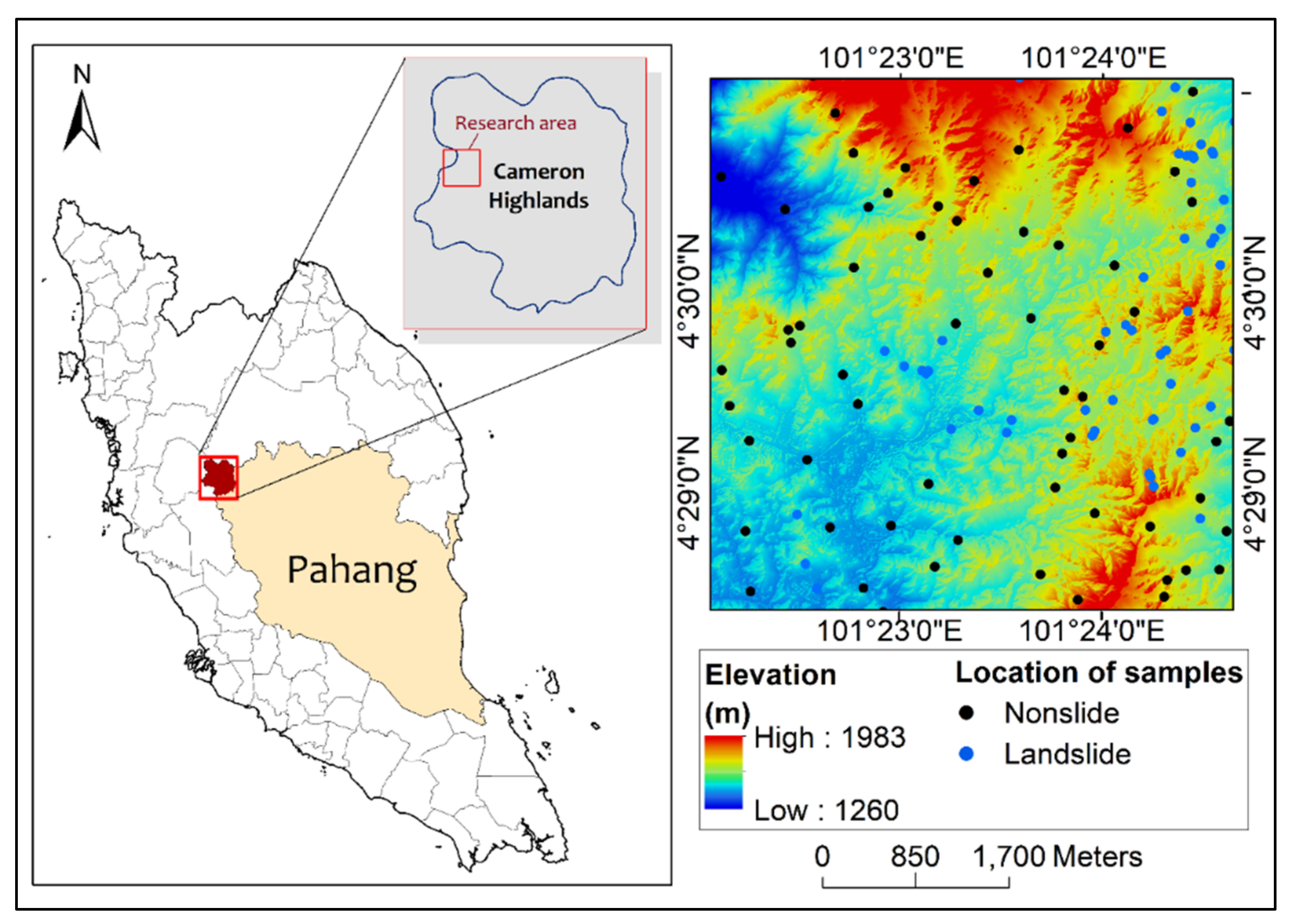
2.1. Study Area

The study area is a sub-area of Cameron Highlands located in the north-eastern tip of Pahang State, Malaysia (latitudes 101°24′00″ E and 101°25′10″ E, longitudes 4°30′00″ N and 4°30′55″ N) (Figure 1). It is a tropical mountainous region with frequent occurrence of landslides and flash flooding triggered by strong, prolonged rainfall [44]. The combination of topography, climate, and human activities creates natural hazards that pose a major threat to Cameron Highlands [20,44]. Government reports and previous research indicate that landslides in this area have been common, and that there has been significant damage to property in the past [20].
Geomorphology of the area is mostly hilly landforms, mainly the western and northern parts. The land slope ranges from 0° to 78° and the lowest and highest altitudes are 1153 m and 1765 m. Forest and tea plantations, temperate vegetables and flower farms are the main vegetation cover of the area. The primary lithology in this area is megacrystic biotite granites, the other geological structures being schists and phyllite [44]. Cameron Highlands has a mild climate with average annual rainfall between March and May and November to December. The average daytime and night-time temperatures are 24 °C and 14 °C, respectively. Approximately 8% (5500 ha) of the area is agricultural land, 86% (60,000 ha) is cultivated, 4% (2750 ha) is housed, and the rest is used for recreation and other activities. The selected sub-area occupies about 25 km2.

2.2. Geospatial Database

Valid datasets are required to assess landslide susceptibility with machine learning methods ranging from digital elevation models, geological data to geographic information system (GIS) data such as stream network, road network, and administrative division/subdivision to historical landslides aka landslide inventory. The datasets collected and prepared in the current research are shown in Table 1. A 0.5 m digital elevation model (DEM) was generated using LiDAR point clouds and down-sampled to 2 m. The details of the LiDAR data and campaign are documented in Table 1. The DEM was generated by removing non-ground points by the Multiscale Curvature Classification (MCC) algorithm [45] and the Inverse Distance Weighted (IDW) interpolation techniques were implemented in ArcGIS Pro 2.4. The DEM is then used to generate other causative factors such as altitude, slope, aspect, plan curvature, profile curvature, ruggedness index, relative topographic position, topographic wetness index, and sediment transport index. Satellite images from Landsat 7/ETM+ were used to generate vegetation density and normalised difference vegetation indices. Geological data such as lithology and lineaments have also been analysed in this study. However, the study area contained only one type of lithology (granite) and was therefore not considered being a factor in the prediction models. Lineament data was used to prepare the distance from lineaments factor using the GIS Euclidean distance function. Additionally, GIS data such as stream and road networks, land use, administrative divisions/subdivisions, and historical landslides, were used to prepare other causative factors and to prepare training and test samples.
This research was conducted using open-source libraries including Numpy, Scikit-learn, and Pandas in Python platform. In addition, ArcGIS Pro 2.4 was implemented for data preparation, spatial analysis, and result presentation. All experiments were conducted in Python using Scikit-Learn and Keras on a computer with a Core i7-4510U CPU running at 2.60 GHz, 16 GB of RAM, and a x64-based processor.

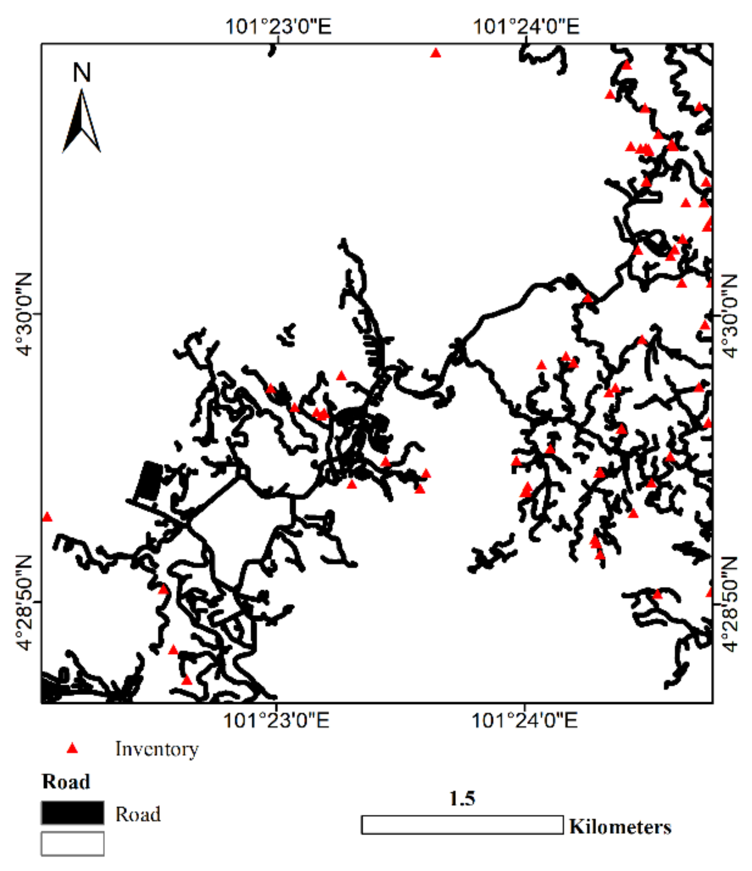
2.2.1. Landslide Inventory

Landslide inventory data is essential for training and validating machine learning and statistical predictive models. A typical landslide inventory database contains information, such as the location of past and recent landslide events, type of landslides, and other statistical information about the landslide sites and their impacts. The landslide inventory data of the area was prepared by [46] in their previous works in the same area. A total of 63 landslides were identified in the area, as shown in Figure 1. The database shows that most of the landslides are shallow rotational and a few translational in type. Landslide data has been randomly split into a training set (80% of the landslides; 50) and test set (20% of the landslide; 13). Table 2 shows the descriptive statistics of landslide causative factors at landslide locations calculated with mean values from a 10 m circular buffers.

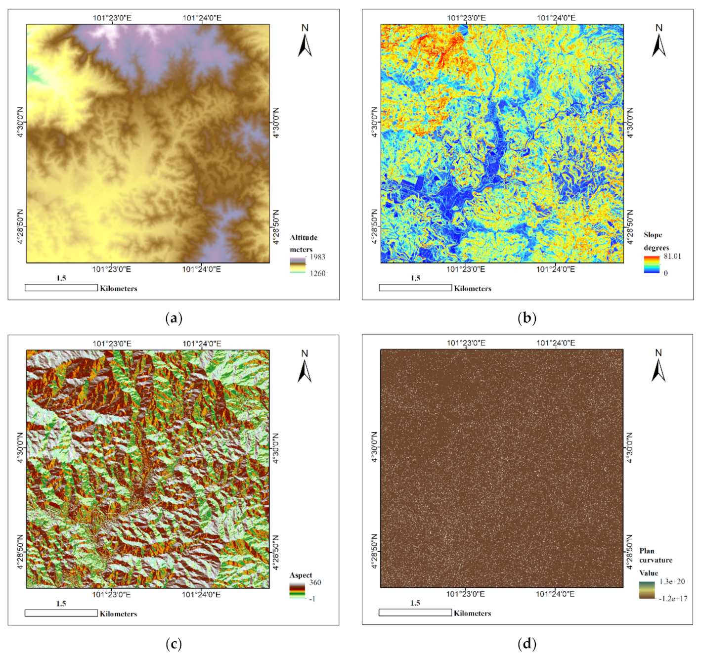
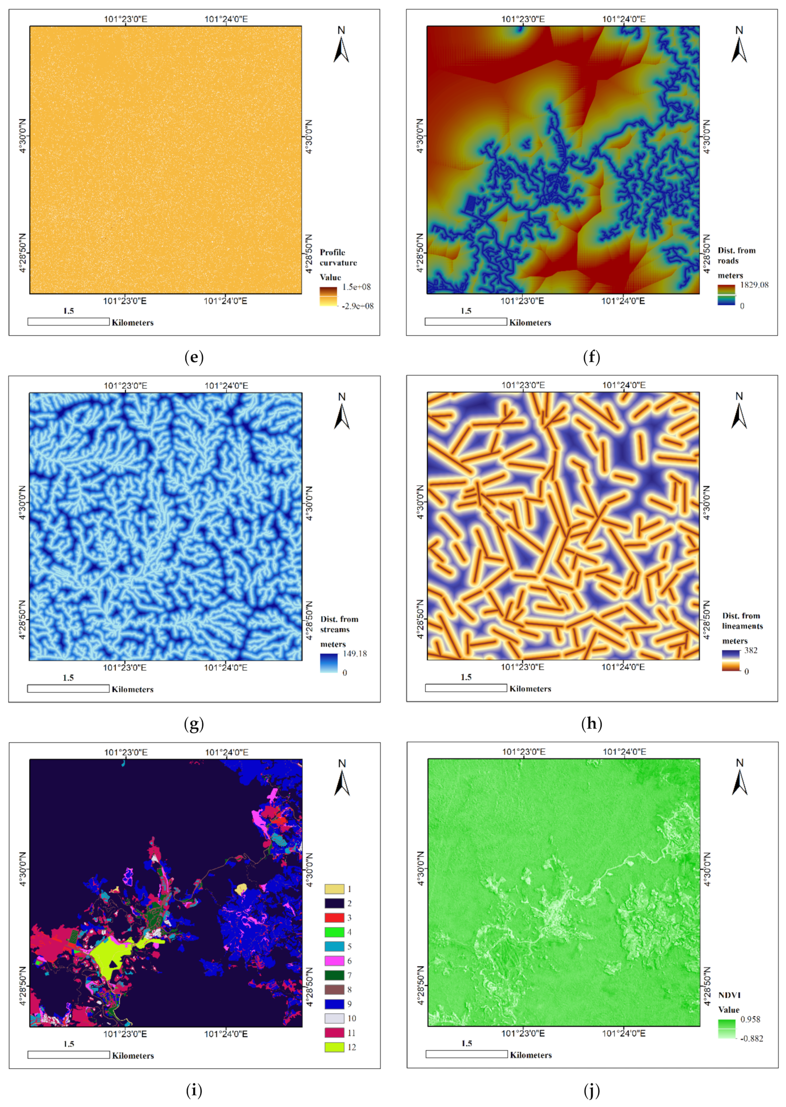
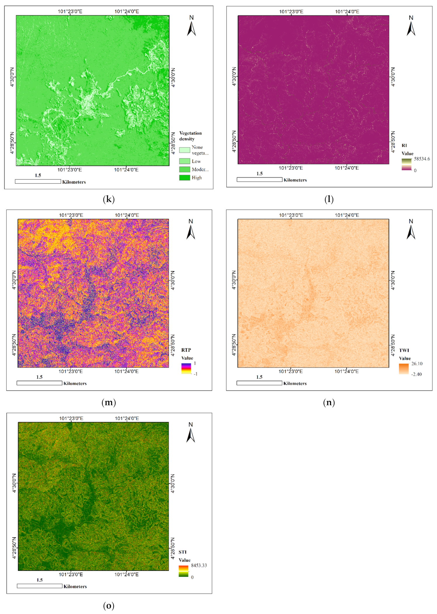
2.2.2. Landslide Causative Factors

This work involved a total of 15 causative factors, two of which were categorical while the others were numerical. All factors were selected based on previous works done in the same area, which showed a significant correlation to landslide events. Although some research indicates that numerical factors should be reclassified from continuous to categorical; this study did not reclassify numerical factors into categorical to allow more reliable calculation of meta-features required in the proposed meta-learning, reduce the predictive model’s sensitivity to the type of reclassification models and range of values used to convert continues values into categorical and reduce the time-complexity of the models as they do not have to do extra processes with new examples during prediction. Thus, two factors, namely vegetation density and land use, as well as 13 numerical factors, as indicated in Table 3, are included in this research (the maps of landslide causative factors are provided in Appendix A). The categorical data were transformed to numerical form. The one-hot encoding was used for the ordinal representation. The integer encoded variable is removed and one new binary variable is added for each unique integer value into the variable. Each category value is converted into a new column in this strategy and assigned a 1 or 0 (representing true/false) value to the column [47].

2.3. Methodology

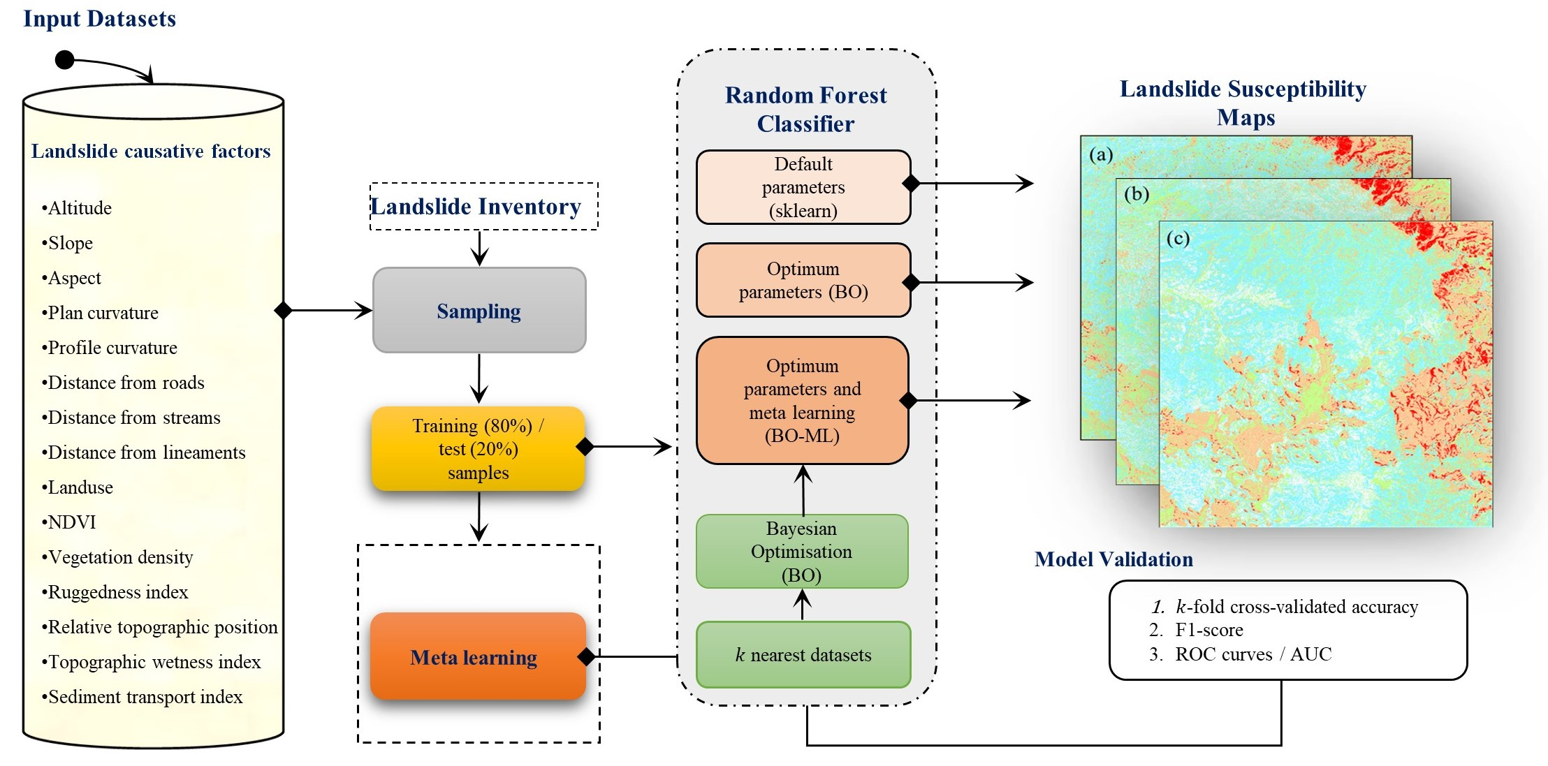
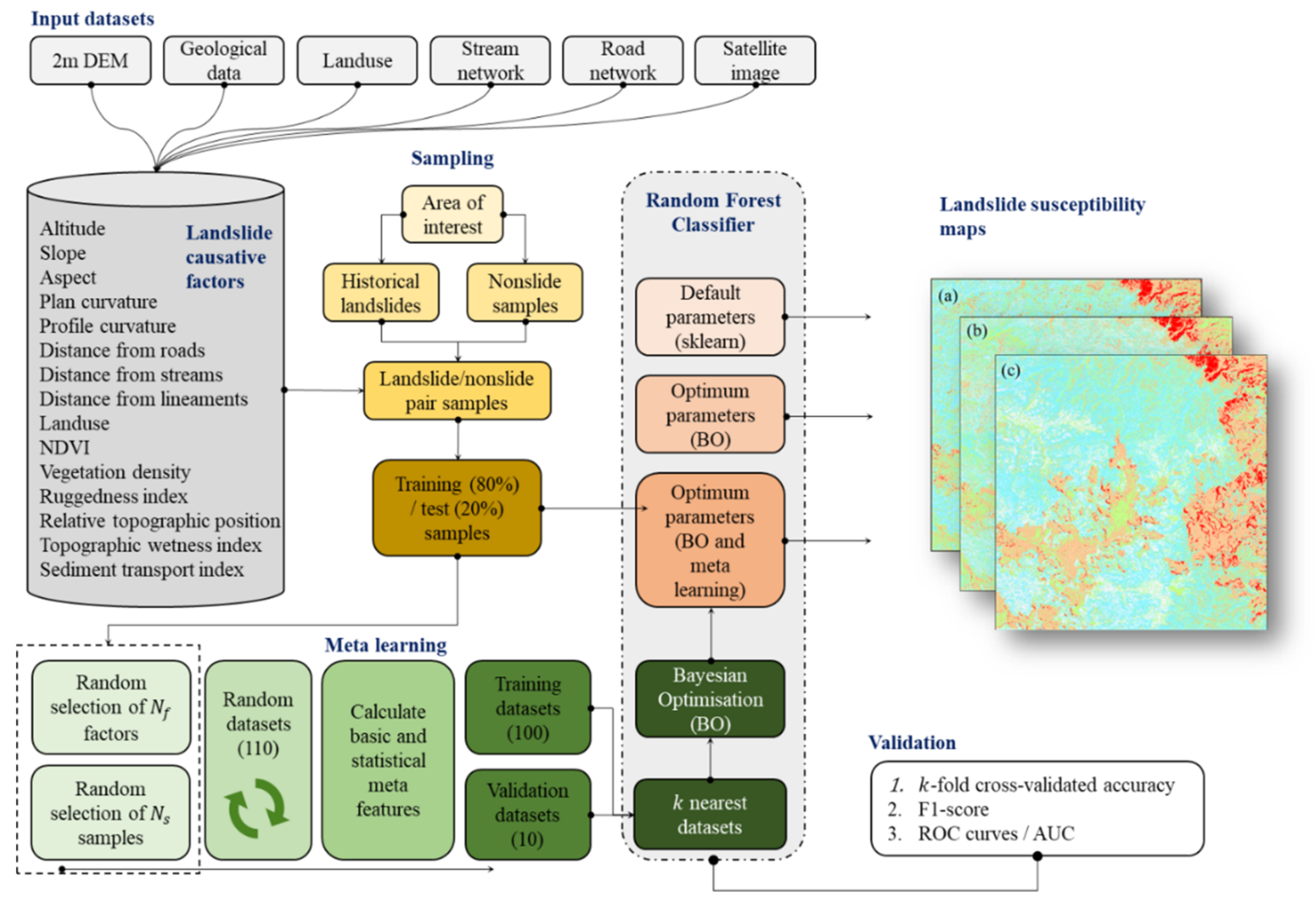
2.3.1. Overall Esearch Methodology

Figure 2 shows the overall methodology for evaluating spatial prediction of landslides using RF and a meta-learning approach for optimising hyperparameters.
Several geospatial datasets were obtained and pre-processed, including a 2 m digital elevation model, geological data (i.e., lineaments), land use, stream network, road network, and satellite images. Following that, a proper geospatial database was developed to include 15 causative factors from the collected datasets. These include altitude, slope, aspect, plan curvature, profile curvature, distance from roads, distance from streams, and distance from lineaments, land use, normalised difference vegetation index, vegetation density, ruggedness index, relative topographic position, topographic wetness index, and sediment transport index. The database also included the research area boundary (area of interest, short AOI) and historical landslides, which are essential to prepare training and test samples for the modelling phase.
In addition to historical landslides, non-landslide samples are required to prepare training and test samples. They are created randomly at far-off locations by a particular distance to existing landslides. The total number of non-slide samples is equal to the number of landslide locations to prevent data set imbalances. The non-slide samples produced are combined with landslide samples to create the training (80%) and test (20%) samples used to train and test the modelling technique. From training samples, 15 percent were held aside to optimise model hyperparameters. The selection process of non-landslide samples should be performed carefully. There are several strategies for selecting training samples in the literature. The fundamental approach is random sampling which we used in this study [10,11]. The non-landslide samples were collected from the rest of the area, exhibiting different features such as buildings, trees, etc. We utilized landslide inventories as a guide to select these non-landslide points. Accordingly, the generation of the non-landslide points was performed randomly via ArcGIS Pro 2.4. tool, satisfying the following conditions. First, any non-landslide sample needs to be buffered at a minimum distance of 500 m away from landslides. Second, the distance between any two non-landslide samples must be more than 100 m.
Three RF models were developed using three different hyperparameter configurations such as (1) default values from sklearn library, (2) best values from Bayesian optimisation (BO), and (3) best values from the proposed meta-learning optimisation method (BO-ML).
To optimise RF hyperparameters with the proposed meta-learning method, the following steps are followed. First, a total of 110 datasets were created by random sample features and samples from the available data. For each dataset, a set of basic and statistical meta-features were calculated. Additionally, for each dataset, the best hyperparameters of RF were obtained through Bayesian optimisation. Each dataset contained a pair of meta-features and best values of hyperparameters. Datasets were then randomly split into training datasets (100) and validation datasets (10). To find best hyperparameter values for a new dataset, k nearest datasets were determined by comparing meta-features with k nearest neighbour algorithm and running Bayesian optimisation by starting from a list of hyperparameter configurations suggested by meta-learning.
Lastly, the model predictive ability was evaluated based on three accuracy metrics, including k-fold cross-validation accuracy (k = 5 in this work), F1-score, and area under the receiving operating characteristic curves (AUROC).

2.3.2. Modelling: Random Forest

Random forest (RF) developed by Breiman, L. [60] in 2001 is a common supervised classification algorithm based on the learning of decision trees [60]. It can also be extended to other tasks such as regression, clustering, and detecting interactions. A forest is formed by constructing several binary trees. Each tree fits a bootstrap sample from the training set with a random subset of features and samples selected at each node to minimize correlation among the generated trees [61]. The random selection of the data set may affect the model’s performance, so using a collection of several trees helps ensure model stability. For each tree grown on a bootstrap sample, the error rate “out-of-bag” (OOB) equal to the standard deviation error between predicted and observed values is calculated using samples left out of the bootstrap sample. OOB samples are also used to establish a ranking of importance for the features. Majority vote of all trees decides the final predictions.
When splitting a node during tree construction using the concept of the largest Gini coefficient, the selected split is no longer the best split among all features [62]. Alternatively, the split is the best split among a random subset of features. Because of this randomness, the bias of the forest typically increases marginally (regarding a single non-random tree bias) [63,64]. Nevertheless, due to averages, its variance often decreases, typically more than compensating for the increase in bias, producing a better overall model.
RF estimates the relative importance and ranks input features concerning the predictability of landslides using features used as decision nodes in the trees [36]. Features used at the top of the tree contribute to the final prediction decision of a larger fraction of the input samples. Thus, the estimated fraction of the samples they contribute to can be used to estimate the relative importance of the features. Here, the fraction of samples a feature contributes to is combined with the decrease in impurity from splitting them to create a normalised estimate of the predictive power of that feature. Other benefits of the RF algorithm include [65]:
  • RF is ideal for working with mixed variables, i.e., both categorical and numerical, most likely in landslide modelling,
  • In RF, each tree has access to specific subspace feature sets. This random selection of features to split each node contributes to a favourable error rate. This randomness also offers high accuracy rates for outliers in predictors, and
  • RF is a good feature engineering tool. That means finding the most relevant features from the training dataset.
The challenge with RF is to optimise a number of hyperparameters to increase efficiency and predictive capacity [66]. The most important parameters include the number of trees in the forest, maximum depth of the trees, the maximum number of features considered at each split, minimum samples required in a leaf, minimum samples required to split a node, and the function to measure split quality (also known as criterion). Selecting optimised values for these parameters can reduce the model’s time complexity, increase model generalization (minimize the OOB error), and produce a more accurate estimation of feature importance. Appendix B contains more information on these parameters [60].

2.3.3. Optimisation: Bayesian Optimisation

This research uses Bayesian optimisation (BO) to determine optimal landslide predictive models-hyperparameters. Unlike grid and random search, BO finds optimum hyperparameters faster, relying on prior knowledge gained through iterations. The algorithm depends on the Gaussian process (GP) model to fit the posterior distribution of an objective function by increasing the number of samples, allowing it to find the optimal solution and optimise the hyperparameter [39]. GP model can easily determine a predictive distribution of objective function. The model’s predictive distribution determines the possible values of the objective function at each point of the input space. By considering this predictive distribution, BO methods guide the search, focusing on those input space regions that are expected to provide the most information about the solution to the optimisation problem.
In this research, BO was used to optimising six RF model hyperparameters as shown in Table 4. It was based on 20 iterations, also known as calls (n). As an objective function, negative minimum AUROC with five-fold cross-validation was used. After each iteration, the better model configuration was found until the 20-call convergence. At the cost of additional processing time, better configurations can be found when looking for larger search spaces.

2.3.4. Proposed Meta-Learning Optimisation Approach

Meta-Learning:
The idea of meta-learning is to find the best values of RF hyperparameters for new datasets based on previous knowledge regarding best hyperparameters. For a new dataset, the Bayesian optimisation, instead of learning from scratch, would begin with hyperparameter configurations that were optimal for the most similar previous datasets. The similarity between datasets can be measured using common distance metrics such as p-norm distance.
Let us denote the best hyperparameter configurations as θ ^ 1 , , θ ^ N for the previously encountered datasets D 1 ,   ,   D N , respectively. For a new dataset, first, the algorithm computes the p-norm distance ( d p ) from this dataset to all the training (encountered) datasets and sort them by increasing distance to the new dataset. The similarity between the datasets was measured based on their meta-features, which can be computed for the training and validation (new) datasets.
d p D i ,   D j = m i m j p    
where d p is the p-norm distance between D i and D j datasets, and m i and m j are the set of meta-features for the two datasets.
Then, t hyperparameter configurations will be determined based on the most t similar datasets based on d p . In this research, t was set to 10. Starting from these best t hyperparameter configurations, Bayesian optimisation will run for 10 calls to find the best hyperparameter values for the new dataset. This will help to save time and computing resources as there will not be a need to search large hyperparameter spaces.
Implemented Meta-Features:
To evaluate the proposed meta-learning approach, a number of basic and statistical meta-features were implemented. This research implemented 13 basic meta-features such as the number of instances and the number of features, describe the basic dataset structure [67]. Further, it implemented 14 statistical meta-features which characterise the data via descriptive statistics such as kurtosis and skewness [68]. Such meta-features can characterize the complexity of datasets providing an evaluation of the performance of the algorithm [69]. Broad data characterization, deep data exploration and various meta-learning-based data assessments can be obtained by extracting numerous meta-feature functions [69]. These meta-features can be general information (e.g., simple measures, number of instances, attributes, and classes) and statistical information (e.g., standard statistical measures describing data distribution and discriminant measures including Min., Max, Standard deviation, Skewness, Kurtosis, etc.). These meta-features can be simply extracted by instantiating the “MFE class” in Python. It calculates a group of meta-features as summary functions to abstract these values. After fitting, the “Extract” method extracts the corresponding measures [70]. The details of these meta-features are given in Appendix C.
Datasets:
The evaluation of the meta-learning optimisation was based on datasets randomly sampled (both factors and samples) from the datasets of Cameron Highlands. A total of 110 datasets were created with a different number of factors and a number of samples. For developing and training the meta-learning models, this research used 100 datasets randomly selected from the generated datasets. The remaining 10 datasets were kept for validating the method. Table 5 shows the shape and the list of causative factors selected in each validation dataset.
For each training dataset, this research first shuffled the samples and then split it in stratified fashion into 80% training and 20% validation. Before training any machine learning model, the dataset needs to be well-shuffled to avoid bias or patterns in the split datasets for training, testing, and validation datasets. If shuffling is neglected, the data can be sorted, or similar data points could lie next to each other, leading to slow convergence.
Moreover, stratified sampling seeks to split a dataset so that every split is similar with respect to datasets to ensure the same distribution of classes on datasets. It is often desired to ensure that the train and test sets have almost a similar percentage of samples of each target class as the complete set.
Then, we computed the validation performance (AUROC) for Bayesian optimisation by five-fold cross-validation using the validation dataset. For each training and validation dataset, the basic and statistical meta-features were computed and stored on disk. As such, the computed datasets stored on the disk were the meta-features and performance of RF with best hyperparameters found by the Bayesian optimisation for the training dataset and only meta-features for the validation datasets.

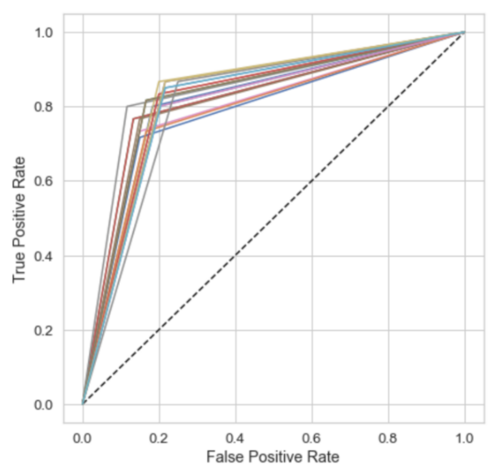
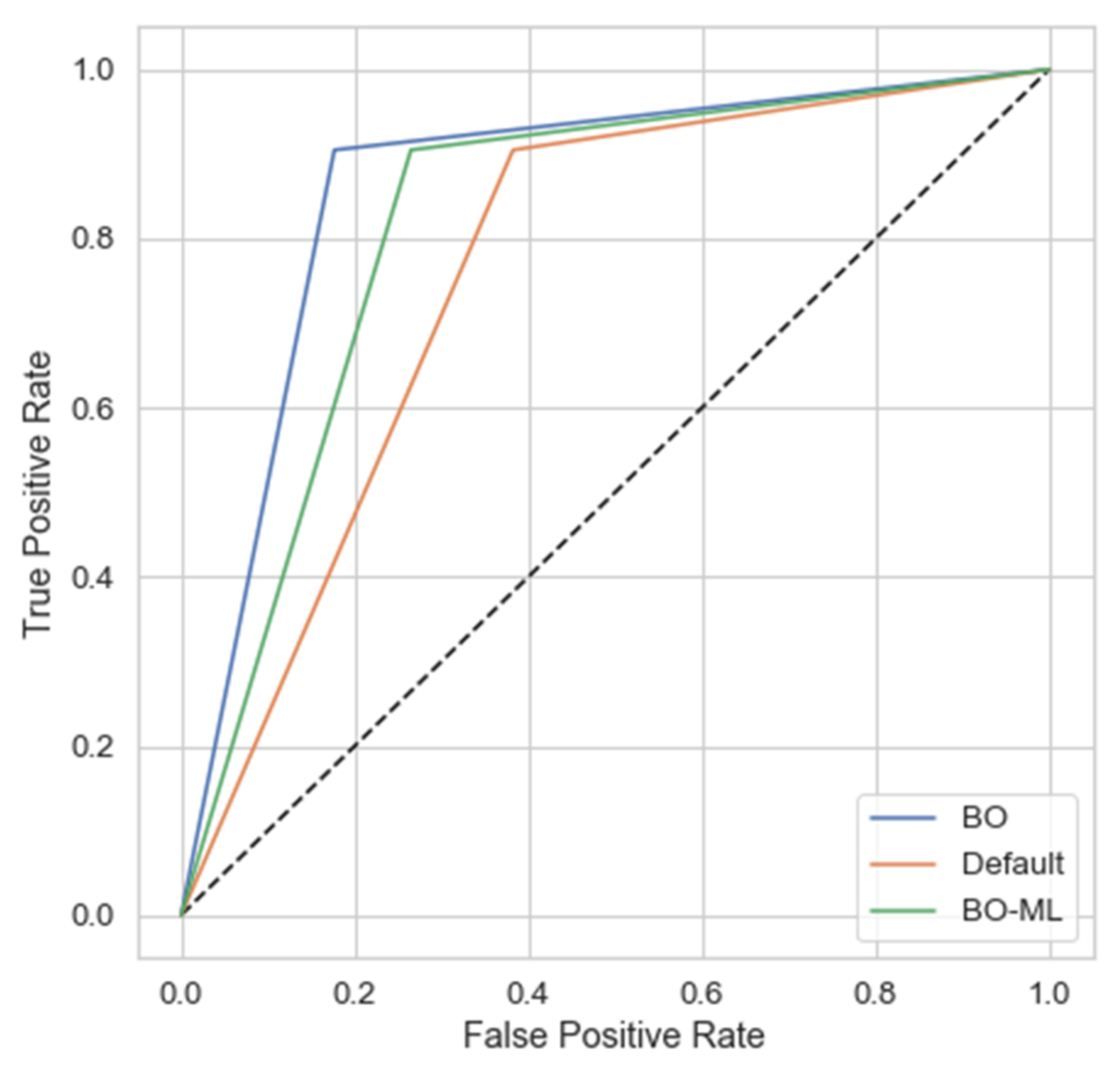
2.3.5. Performance Assessment

The performance of the proposed models was evaluated using three standard accuracy metrics including k-fold cross-validated accuracy, F1-score, and area under receiving characteristic curves (ROC) (i.e., AUROC).
k-fold cross-validated accuracy:
Accuracy is the most common metric for classification tasks, including landslide susceptibility mapping. It is the fraction of the correctly predicted sample and can be calculated using the following equation [71]:
A c c u r a c y = T P + T N T P + T N + F P + F N              
where T P is true positive, the number of positive samples correctly predicted, T N is true negative, the number of negative samples correctly predicted, F P is false positive, the number of positive samples wrongly predicted as negative, and F N is false negative, the number of negative samples wrongly predicted as positive.
To avoid miscalculating the accuracy of a model, it is suggested to use k-fold cross-validation, which is a model validation approach based on partitioning the data into k subsets (k = 5 in this research). The basic idea behind this approach is to hold a set at a time and train the model on the remaining set. Then, test the model on hold out set. However, accuracy is not always the best metric for evaluating classification models because it does not care about positive events. Therefore, additional metrics are often used to explain the performance of the proposed models.
F1-score:
The F1-score is the harmonic mean of recall ( r ) and precision ( p ), with a higher score as a better model. Precision ( p ) is determined by dividing the true positives (number of landslide pixels) with the total number of pixels classified as a landslide. The sensitivity (r) is the degree of true positives correctly predicted and distinguished and can be defined as the number of true positives divided by the total number of pixels belonging to the landslide class. The F1-score is calculated using the following equation [72]:
F 1 - s c o r e = 2 × p   ×   r p + r
p =   T P   T P + F P  
r =   T P   T P + F N
The problem with the F1-score metric is assuming a 0.5 threshold for selecting which samples are predicted as positive. Changing this threshold would change performance metrics. ROC curve is a very common method to solve this problem.
ROC curves and AUROC:
ROC, a graphical representation of model success and predictive accuracy, is another important accuracy metric often used to assess models of landslide susceptibility. The area under ROC is known as AUROC, a quantitative measure summarizing model performance. ROC curves help to understand the balance between true-positive and false-positive rates. A perfect model has 1.0 AUROC, and 0.5 AUROC indicates random models. The closer the AUROC to 1.0, the higher the model’s performance [73].
ROC curves plot y-axis sensitivity and x-axis specificity, corresponding to decision thresholds [74,75]. AUROC calculates a trapezoidal equation as follows:
A U R O C = 1 2 i = 1 n 1 T i + 1 T i C i + 1 + C i 2 B  
where T i is the i th percent landslide susceptibility, C i is the i th cumulative percentage of landslide occurrence, n is the number of the percent landslide susceptibility index value, and B is the baseline value (i.e., B is usually equal to zero).

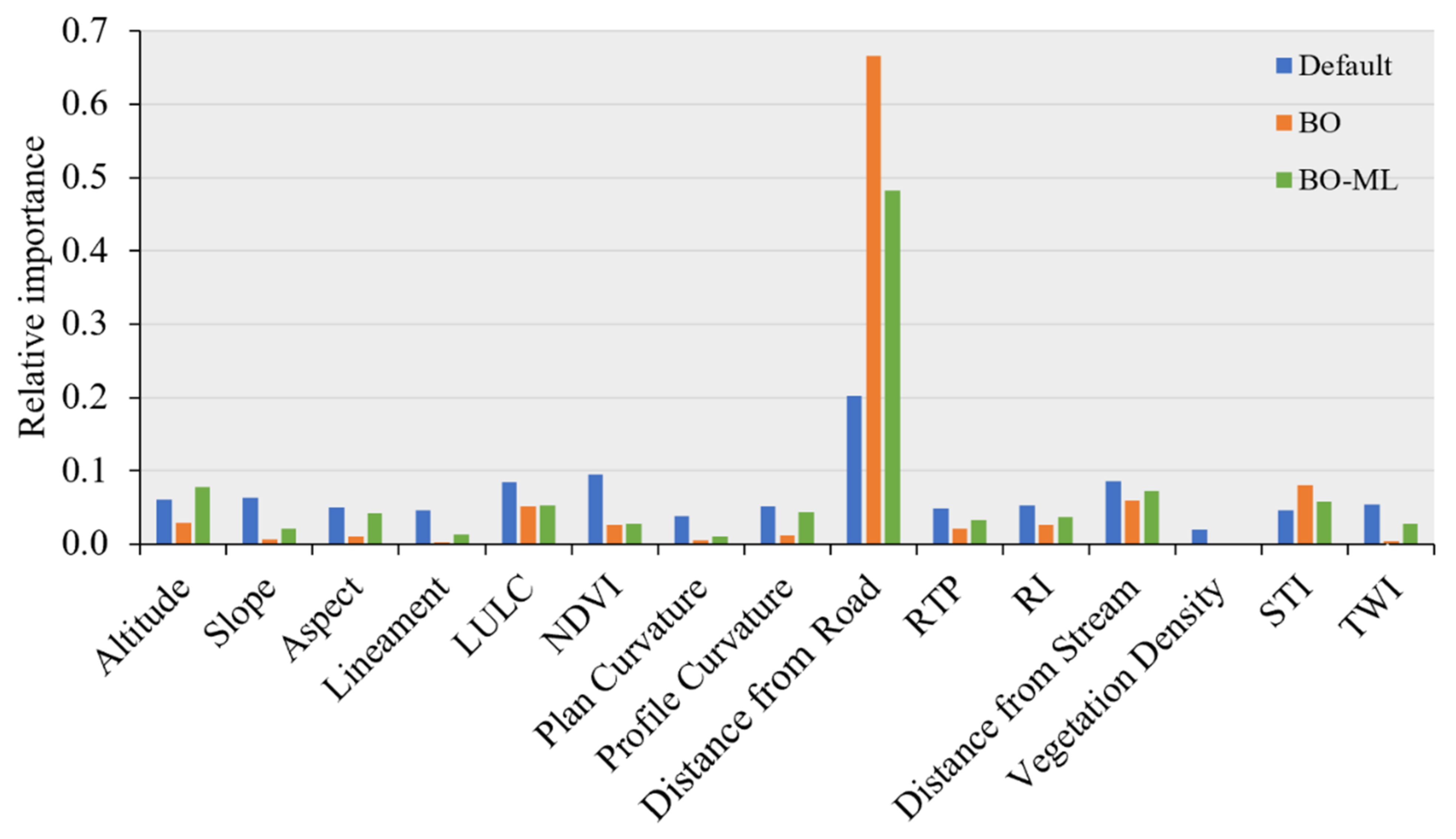
2.3.6. The Relative Importance of Causative Factors

The influence of every conditioning factor on the occurrence of landslides varies [76,77]; thus, examining the importance of the factors for landslide occurrence can provide valuable information. To date, there is no agreement on the selection of reliable landslide conditioning factors due to the complexity of landslides [7,78]. However, several strategies can support the identification of the most and least contributing factors. RF is a popular technique that is widely used for this purpose due to its ability to feature importance/selections.
Multicollinearity can occur when a predictor variable in a multiple regression model can be linearly predicted from the others with superior accuracy. However, decision trees algorithms (such as RF) are resistant to multicollinearity or outliers by nature [79]. Moreover, the success of a meta-learning technique significantly relies on the quality and quantity of the meta-data features employed for learning. To well characterize the meta-data, a collection of many meta-features discriminating among various learning tasks is needed [79]. This ability of meta-learning can offer a better generalization to other areas with almost similar geo-environmental and topographical characters. Nevertheless, we have selected the most essential and best available causing factors based on the previous projects in the study area [20].
In the present study, we used RF as the standard algorithm for the modelling, as the accuracy of RF is not certainly affected by the multicollinearity loads [80,81,82,83]. In fact, this is one of the main advantages of RF, which meta-learning could benefit and learn from the features in a convenient scheme.

3. Results

This paper developed a meta-learning approach to optimising RF models for the assessment of landslide susceptibility at Cameron Highlands. This proposed approach was compared to RF with default hyperparameter settings (sklearn) and Bayesian optimisation to evaluate its predictive ability.

3.1. Performance of RF with Default Values of Hyperparameters

Table 6 shows the default values of the critical RF hyperparameters taken from the sklearn software package (https://scikit-learn.org, access on 1 September 2020). RF, with these default values, achieved AUROC of 0.779 and 0.761 for the training and test datasets, respectively. Comparing the default model with random models on the test dataset achieved AUROC of 0.742 ± 0.015 for 20 randomly sampled parameters. Figure 3 shows the ROC plots of these random models. The results suggest that RF with the default parameters compares to a random model, indicating the need to optimise these critical parameters systematically to produce more accurate landslide predictions.

3.2. Performance of RF with Optimised Values of Hyperparameters

Table 7 shows the performance of the RF model with two optimisation methods, i.e., Bayesian method and the proposed meta-learning based approach compared to the model with the default parameters. Considering the five-fold cross-validation accuracy metric, the Bayesian method achieved the best performance for both the training (0.810) and test (0.802) datasets. The meta-learning approach achieved slightly lower accuracies than the Bayesian method for the training (0.769) and test (0.800) datasets. The model with the default parameters achieved the worse performance. Similarly, the Bayesian method outperformed the other two models based on F1-score on both the training and test datasets. Based on this metric, the meta-learning approach (BO-ML) also achieved better results than the model with the default parameters. Finally, based on the AUROC metric, the models with optimised parameters either by the Bayesian or meta-learning methods produced more accurate landslide predictions than the model with the default parameters of the sklearn. Figure 4 illustrates the ROC plots of the three investigated models using the test dataset.
To further evaluate the proposed meta-learning optimisation method, Table 8 shows the best hyperparameter settings obtained by the Bayesian method for the 10 validation datasets (see Section 2.3.4). These best hyperparameter configurations were obtained based on the search space given earlier in Table 4. The performance of the three RF models (i.e., default parameters, Bayesian method, meta-learning approach) are given in Table 9 for the training dataset and Table 10 for the test dataset using the three different evaluation metrics, i.e., five-fold cross-validation accuracy, F1-score, and AUROC.

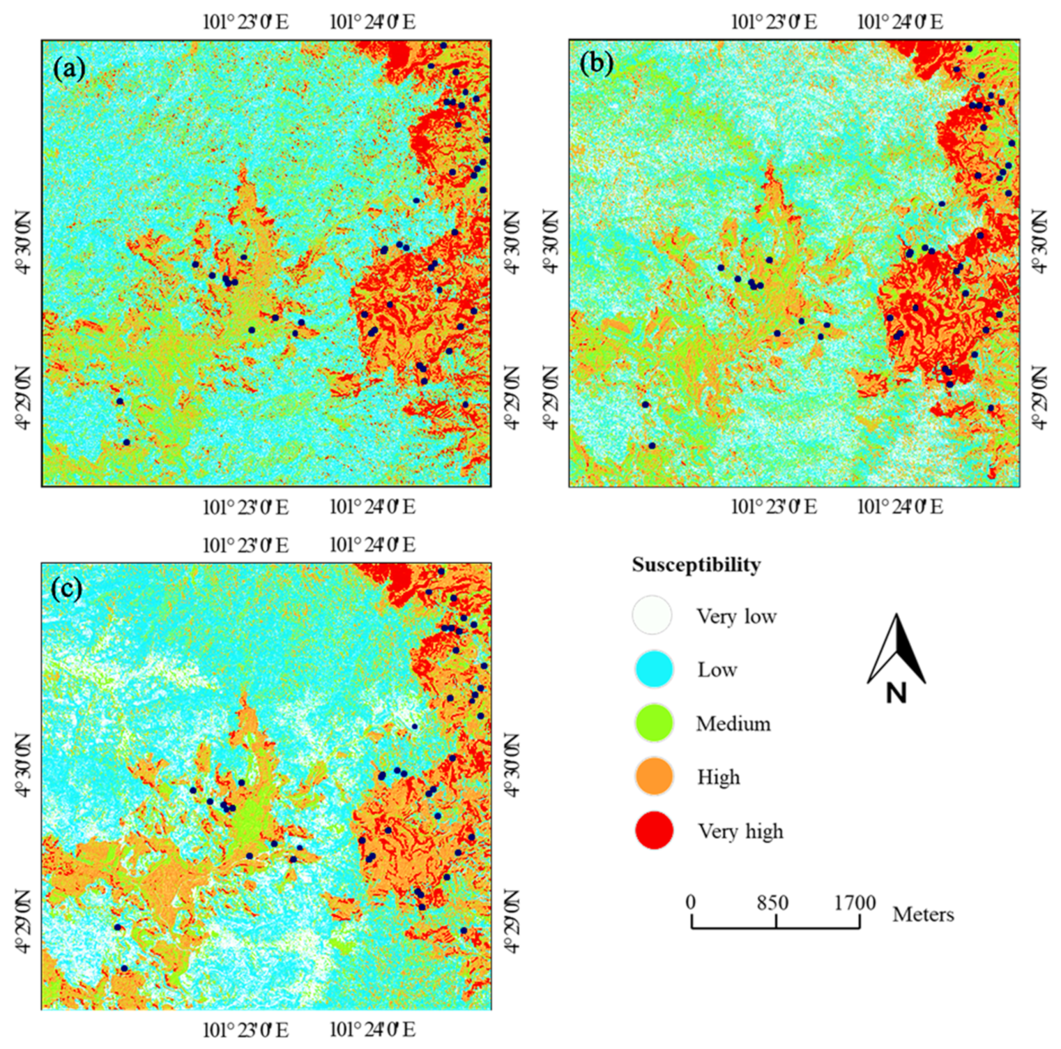
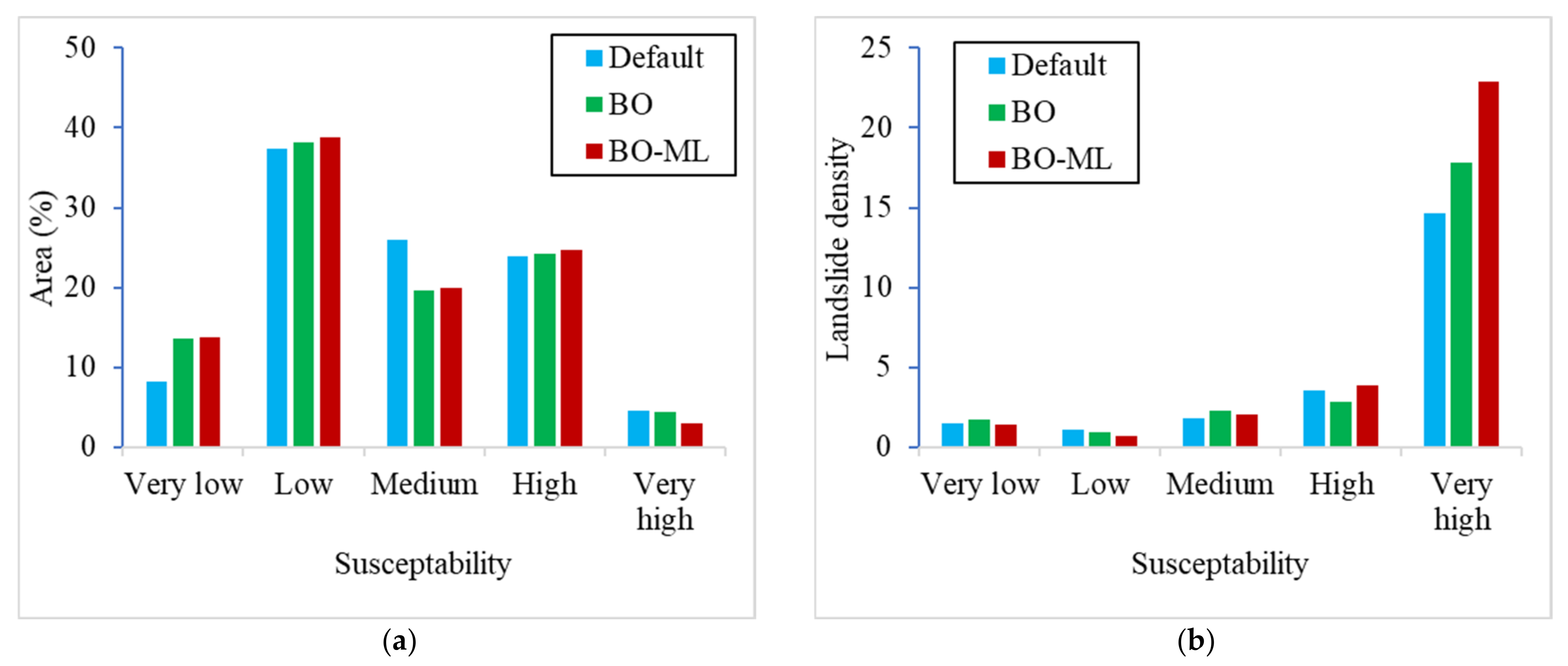
3.3. Landslide Susceptibility Maps

The successfully tested models were used along with the training dataset to prepare the landslide susceptibility maps of the study area. For each pixel, the probability of landslide occurrence was computed using RF with the default parameters, Bayesian method, and the proposed meta-learning approach. The resulted data was used in GIS and the three susceptibility maps were produced. The maps were reclassified into five susceptibility classes, namely very low, low, moderate, high, and very high susceptibility using the natural break classification method implemented with the ArcGIS Pro 2.4 function (Figure 5). Then, the number of landslides were identified in each susceptibility class in the produced susceptibility maps to quantify the landslide density (number of landslides/susceptibility class area). Figure 6 shows the area in pixels of the five susceptibility classes and the landslide density graphs based on the results from the three tested models. The three models identified the largest number of landslides in the higher susceptibility classes. Higher susceptibility values found in areas with high altitudes, far from roads, and close to streams.
As the five susceptibility levels by the natural break classification approach are based on the histogram of data distribution, the classes were therefore distributed within the five class ranges as (very-low (<0.2), low (0.2–0.4), moderate (0.4–0.6), high (0.6–0.8), and very-high (>0.8) which is common in natural break classification [84]. Figure 6a shows that almost more than 51% of the area belongs to very-low and low classes, while almost 3% of the area ranges in a very-high susceptible area which seems logical within the study area. More importantly, as is shown in the landslide density graph in Figure 6b, the historical landslides mostly fell into the high and very-high susceptibility regions, revealing a good correspondence with the map generated by the present meta-learning approach (BO-ML).

4. Discussion

LSMs are essential tools for managing landslide-prone areas. The models are also required to have a high predictive ability and be stable to be used successfully by governmental agencies to develop landslide risk strategies. This paper contributes to the improvement of RF models with Bayesian optimisation and meta-learning for accurate landslide susceptibility mapping at Cameron Highlands. Unlike existing studies which optimise machine learning models from scratch, the proposed optimisation approach starts with promising hyperparameter configurations that performed well on encountered datasets. This approach saves time and computing resources as it runs at fewer iterations compared to other grid and Bayesian methods.
This research used RF as a prediction model because it showed a encouraging performance and stable predictions in previous studies [15,24,85]. In the present study, as meta-learning begins with promising configurations based on several basic and statistical meta-features, RF appears an attractive method for dealing with such meta-features. It searches for the best feature among a random subset of features instead of searching for the most critical feature while splitting a node, which provides additional randomness to the model. Moreover, it is a powerful method that is less sensitive to multicollinearity, noise, and outliers since it employs random features for the modelling [86,87]. These random features in the learning process make the overfitting issue to be minimal. Another advantage is its ability to recognize the most and least important causing factors, which is an additional benefit to support the aim of the present work.
Since RF can assess the relative importance of the landslide causative factors, we looked at how it performs with different hyperparameter configurations. Figure 7 shows the relative importance of the causative factors obtained by the default model, Bayesian method, and the proposed meta-learning approach.
The three models agreed that the distance from roads and vegetation density are the most and least important causative factors regarding the predictability of landslides in the study area, respectively. These results were also confirmed as most of the landslides have occurred along the roadside (Figure 8).
The default model identified NDVI and distance from streams as the second and third most important factors and plan curvature and distance from lineaments as the second and third least important factors. Instead, the Bayesian method showed that STI and distance from streams are the second and third most important factors. This model also showed that distance from lineaments and TWI are the second and third least important factors in the study area, respectively. Finally, the meta-learning approach calculated altitude and distance from streams as the second and third most important factors. This approach agreed with the default model that the plan curvature and distance from lineaments are the second and third least important factors regarding the predictability of landslides in Cameron Highlands. While the three models agree on some factors as the most or least important in the study area, further analyses should be carried out if computing factor importance is the research focus rather than the accuracy of landslide predictions.
However, the same meta-learning approach can be used to optimise other machine learning models, especially those require extensive computing power, e.g., neural networks and ensemble models. The meta-learning optimisation can also be a promising solution when many models need to be tested as it provides faster optimisation to those models.
Meta-learning also can be used with other optimisation methods other than Bayesian techniques such as evolutionary approaches [40]. As those are already being tested for landslide prediction, it could be worth exploring meta-learning with such optimisation techniques. Since the application of meta-learning as an approach of optimisation is very rare in landslide prediction studies, advances in these techniques can improve the accuracy and efficiency of landslide prediction models which ultimately can lead to better landslide risk management.
This research confirms that optimising the RF hyperparameters can lead to more accurate prediction of landslides. The use of Bayesian optimisation with RF yielded more accurate predictions by ~7% (five-fold cross-validation accuracy), ~0.125 F1-score, and ~0.103 AUROC compared to the model with default parameters. The meta-learning approach achieved predictions better than the default model by ~6.8% (five-fold cross-validation accuracy), ~0.105 F1-score, and ~0.059 AUROC. The critical parameters of RF investigated and optimised in this research have controls to model bias, variance, and overfitting issues, which explains why the optimised parameters yield more accurate predictions than the default parameters. The results highlight the importance of integrating optimisation techniques such as Bayesian and meta-learning to RF and possibly other machine learning models to achieve significant improvements in preparing landslide susceptibility maps. Other related studies also reported improvements to the RF [39] and deep learning methods [33] with Bayesian optimisation for landslide susceptibility assessment.
Although the Bayesian optimization and meta-learning optimization techniques were relatively close to each other, BO-ML was successfully able to identify the largest number of landslides in the higher susceptibility classes as per density graphs in Figure 6b, which is a promising result. From another side, the Bayesian optimization effectively tunes a few hyper-parameters; however, its productivity reduces a lot when the search dimension grows in large amounts, leading to a situation where it is at the same level as random search [88]. In addition, it can suffer from a high computational cost if the number of evaluations is high.
Nevertheless, the proposed optimisation approach starts with promising hyperparameter configurations that performed well on encountered datasets. This approach saves time and computing resources as it runs at fewer iterations compared to other methods. As the meta-learning optimisation technique is very limited in the landslide prediction, advances in these techniques can boost the accuracy and efficiency of landslide modeling, especially when the data are large and more complex that needs a massive processing time. It can improve model generalization and produce a more accurate estimation of contributing factors. In addition, in previous studies, the prior knowledge extracted from those techniques was not used to optimise prediction models, but rather optimal values were found by searching large hyperparameter search spaces. It is therefore simple to execute and can be quickly utilized to off-the-shelf hyperparameter optimizers.
As a guideline for employing meta-learning in landslide prediction domain, the selected set of meta-features represents a first footstep in the direction of the meta-learner design, which is capable of suggesting the proper bias for base-learning in landslide studies. To generate such a meta-learning scheme, we recommend the researchers further evaluate the chosen meta-features’ applicability in characterizing diverse learning domains, including groups of related features that need to be considered.
As a limitation of the study, as with any machine learning algorithm, the success of a meta-learning technique significantly relies on the quality of the meta-data employed for learning. To characterize meta-data, a compilation of many meta-features, discriminating among various learning tasks is to be identified/considered. Additionally, careful analysis and usage are needed as complex models need more time to adapt; therefore, it could be challenging to assess their final operation in the early stages of learning.

5. Conclusions

A large number of previous studies have optimised the spatial prediction of landslides. The knowledge extracted in such studies may play a significant role in studies in areas with similar topographic and geological characteristics. However, this prior knowledge was not used to optimise prediction models, but rather optimal values were found by searching large hyperparameter search spaces. This paper introduced the use of meta-learning to optimise spatial prediction, improving the optimisation process of spatial prediction models of landslides. The approach was based on a set of spatial and statistical meta-features for input data, which can be easily calculated for a given datasets. In this way, the optimisation algorithms can be directed towards the optimal values of the hyperparameters faster and as a result yielding improved optimisation.
To test the proposed approach, RF was used as a benchmark prediction model for its generalisation ability and based on previous studies as it often achieved accurate predictions. The meta-learning optimisation was used to find best values of critical parameters of the model can be compared to a benchmark method (Bayesian optimisation) and the model with default values of parameters commonly used in machine learning tools such as Python’s scikit-learn library. Experiments on comparing RF with default parameters to a random model suggested the need to optimise critical parameters systematically. Based on the AUROC metric, optimised models (Bayesian or meta-learning) produced more accurate results than the model with the default parameters.
Despite the successful landslide prediction results obtained in this research with Bayesian and meta-learning optimisation techniques, further research is required to identify and implement more specific meta-features to landslides and spatial data, i.e., spatial distribution, spatiotemporal data clusters, landslide types, and landslide geometry. The more meta-features, the more accurate estimation of data similarity can be obtained which will result in better identification of suboptimal hyperparameter values. As a result, the prediction models can be more accurately and reliably be optimised and used on new datasets.
Overall, advancing our understanding of hyperparameter optimisation of a landslide prediction model can have a positive impact on decision making for planning and managing landslide-prone areas. By implementing a proper meta-learning scheme, further generalized state-of-the-art models can be developed for the landslide modelings. Although, in this research, we conducted a comparative study on a relatively small region, implementing the model on even larger configuration spaces can be considered to assess the model’s exportability. Furthermore, the study could be simulated in other topographical set-ups with a variety of factors and different kinds of landslides (e.g., debris flow, rockfall, deep-seated landslides, etc.).

Author Contributions

Project administration, B.P.; Conceptualization, B.P. and M.I.S.; Data acquisition and curation, B.P.; Methodology, M.I.S. and H.A.H.A.-N.; Modelling and data analysis: M.I.S. and H.A.H.A.-N.; Writing original draft: M.I.S. and B.P.; Revised manuscript: H.A.H.A.-N. and B.P.; Supervision: B.P.; Validation: B.P.; Visualization: B.P.; Resources: B.P. and A.M.A.; Review & Editing: B.P., D.S., H.-J.P. and A.M.A.; Funding acquisition: B.P. and A.M.A. All authors have read and agreed to the published version of the manuscript.

Funding

This research is funded by the Centre for Advanced Modelling and Geospatial Infor-mation Systems (CAMGIS), Faculty of Engineering and Information Technology, the University of Technology Sydney, Australia. This research was also supported by Researchers Supporting Project number RSP-2021/14, King Saud University, Riyadh, Saudi Arabia.

Institutional Review Board Statement

Not applicable.

Informed Consent Statement

Not applicable.

Data Availability Statement

Raw data were generated at University of Technology Sydney, Australia. Derived data supporting the findings of this study are available from the corresponding author [Biswajeet Pradhan] on request.

Acknowledgments

The authors would like to thank the Faculty of Engineering and Information Technology, the University of Technology Sydney for providing all facilities during this research. We are also thankful to the Department of Mineral and Geosciences, the Department of Surveying Malaysia, and the Federal Department of Town and Country Planning for providing the LiDAR dataset.

Conflicts of Interest

The authors declare no conflict of interest.

Abbreviations

LiDARlight detection and ranging
RADARradio detection and ranging
CNNconvolutional neural networks
RNNrecurrent neural networks
BObayesian optimization
BO-MLbayesian optimization via meta-learning
ANNartificial neural network
SVMsupport vector machine
RFrandom forest
MFOmoth flame optimiser
DEMdigital elevation model
MCCmultiscale curvature classification
IDWinverse distance weighted
NDVInormalised difference vegetation index
RIruggedness index
RMSDroot-mean-square-deviation
RTPrelative topographic position
TWItopographic wetness index
STIsediment transport index
AOIarea of interest
AUROCreceiving operating characteristic curves
OOBout-of-bag
GPgaussian process

Appendix A

Figure A1. Landslide causative factors used in this research; (a) altitude, (b) slope, (c) aspect, (d) plan curvature, (e) plrofile curvature, (f) distance from roads, (g) distance from stream (h) distance from lineaments, (i) landuse, (j) NDVI, (k) vegetation density, (l) RI, (m) RTP, (n) TWI, (o) STI.
Remotesensing 13 04521 g0a1aRemotesensing 13 04521 g0a1bRemotesensing 13 04521 g0a1c

Appendix B

Table A1. List of the most critical hyperparameters of RF.
ParameterExplanationNecessity of Tuning
Number of estimators or treesNumber of trees to create the RF.At higher numbers of trees, the RF is relatively stable, but at one point it can still overfit and time complexity of the model can increase. This should be tuned.
CriterionFunction to measure split quality. Gini impurity and information gain are two common functions.Both Gini and information gain impurity metrics work well. However, the latter is more computationally heavy due to the log in the Entropy equation.
Maximum depthTree’s maximum depth. The longest path between root and leaf node or max number of splits possible within each treeSince this parameter is used to control over-fitting as higher depth allows the model to learn very detailed relationships to a particular sample, it should be tuned.
Maximum featuresNumber of features to consider when looking for best splitting. These are randomly selected.The square root of the total number of features is suggested as a thumb-rule. The lower is greater for the reduction of variance, however, the bias will increase. Higher values can lead to over-fitting. It should, therefore, be tuned.
Minimum samples leafDefines the minimum samples required in a terminal node or leaf.This can smooth the model. A smaller leaf makes the model more prone to capturing noise in train data and should, therefore, be tuned.
Minimum samples splitSpecifies the minimum number of samples required for splitting in a node.To control over-fitting. Higher values prevent a model from learning relationships that could be very specific to the particular sample selected for a tree. Too high values can also contribute to underfitting.

Appendix C

Table A2. List of implemented meta-features.
Meta FeaturesEquationExplanationRationale
Basic features (simple features related to dataset attributes)
Nr instances n The number of samples in the dataset.Speed, Scalability
Log Nr instances log n Natural log of the number of samples.
Nr features p The number of causative factors in the dataset.Curse of dimensionality
Log Nr features log p Natural log of the number of causative factors.
Nr numeric features p n u m . The number of causative factors that are numeric.Complexity, imbalance
Nr categorical features p c a t . The number of causative factors that are categorical.
Ratio numerical/nominal p n u m . p c a t . The ratio between numerical to categorical factors.Complexity, imbalance
Ratio nominal/numerical p c a t . p n u m . The ratio between the categorical to numerical factors.
Dataset ratio p n The ratio between the numbers of factors to the number of samples.Curse of dimensionality
Log dataset ratio log p n Natural log of the dataset ratio (Number of causative factors divided by number of samples).
Inverse dataset ratio n p The ratio between the numbers of samples to the number of factors.
Log inverse dataset ratio log n p Natural log of the inverse dataset ratio (Number of samples divided by number of causative factors).
Num. symbols c The number of unique labels in categorical factors.Complexity, imbalance
Statistical features (features describe statistical properties of the dataset)
Kurtosis E X μ X 4 σ X 4 List of kurtosis values for the causative factors. It identifies as whether the tails of data distribution of a given X values contain extreme values. The distributions with large kurtosis values are ones where there is the possibility of extreme values, and vice versa.Feature normality
Kurtosis (min) min Kurtosis Minimum kurtosis.
Kurtosis (max) max Kurtosis Maximum kurtosis.
Kurtosis (mean) Kurtosis / p Mean kurtosis.
Kurtosis (std.) σ Kurtosis Standard deviation kurtosis.
Skewness E X μ X 3 σ X 3 List of skewness values for the causative factors. It defines the measure of the symmetry of data distribution for a given X value. When X is far below its mean ( X µ x ) 3 is a big negative number, and when X is far above its mean
( X µ x ) 3 is a big positive number.
Feature normality
Skewness (min) min Skewness Minimum skewness.
Skewness (max) max Skewness Maximum skewness.
Skewness (mean) Skewness / p Mean skewness.
Skewness (std.) σ Skewness Standard deviation skewness.
Minimums m i n Minimum values of the causative factors. Locality, Data distribution
Maximums m a x Maximum values of the causative factors.
Means μ Mean values of the causative factors.
Stds σ Standard deviation values of the causative factors.

References

  1. Zhu, Q.; Chen, L.; Hu, H.; Xu, B.; Zhang, Y.; Li, H. Deep Fusion of Local and Non-Local Features for Precision Landslide Recognition. arXiv 2020, arXiv:2002.08547. [Google Scholar]
  2. Froude, M.J.; Petley, D.N. Global fatal landslide occurrence from 2004 to 2016. Nat. Hazards Earth Syst. Sci. 2018, 18, 2161–2181. [Google Scholar] [CrossRef] [Green Version]
  3. Xie, W.; Nie, W.; Saffari, P.; Robledo, L.F.; Descote, P.Y.; Jian, W. Landslide hazard assessment based on Bayesian optimization–support vector machine in Nanping City, China. Nat. Hazards 2021, 109, 931–948. [Google Scholar] [CrossRef]
  4. Zhou, C.; Lee, C.; Li, J.; Xu, Z. On the spatial relationship between landslides and causative factors on Lantau Island, Hong Kong. Geomorphology 2002, 43, 197–207. [Google Scholar] [CrossRef]
  5. Weng, M.-C.; Wu, M.-H.; Ning, S.-K.; Jou, Y.-W. Evaluating triggering and causative factors of landslides in Lawnon River Basin, Taiwan. Eng. Geol. 2011, 123, 72–82. [Google Scholar] [CrossRef]
  6. Jebur, M.N.; Pradhan, B.; Tehrany, M.S. Optimization of landslide conditioning factors using very high-resolution airborne laser scanning (LiDAR) data at catchment scale. Remote Sens. Environ. 2014, 152, 150–165. [Google Scholar] [CrossRef]
  7. Chang, K.-T.; Merghadi, A.; Yunus, A.P.; Pham, B.T.; Dou, J. Evaluating scale effects of topographic variables in landslide susceptibility models using GIS-based machine learning techniques. Sci. Rep. 2019, 9, 12296. [Google Scholar] [CrossRef] [Green Version]
  8. Kanungo, D.; Arora, M.; Sarkar, S.; Gupta, R. A comparative study of conventional, ANN black box, fuzzy and combined neural and fuzzy weighting procedures for landslide susceptibility zonation in Darjeeling Himalayas. Eng. Geol. 2006, 85, 347–366. [Google Scholar] [CrossRef]
  9. Luo, X.; Lin, F.; Zhu, S.; Yu, M.; Zhang, Z.; Meng, L.; Peng, J. Mine landslide susceptibility assessment using IVM, ANN and SVM models considering the contribution of affecting factors. PLoS ONE 2019, 14, e0215134. [Google Scholar] [CrossRef]
  10. Conoscenti, C.; Rotigliano, E.; Cama, M.; Caraballo-Arias, N.A.; Lombardo, L.; Agnesi, V. Exploring the effect of absence selection on landslide susceptibility models: A case study in Sicily, Italy. Geomorphology 2016, 261, 222–235. [Google Scholar] [CrossRef]
  11. Erener, A.; Sivas, A.A.; Selcuk-Kestel, A.S.; Düzgün, H.S. Analysis of training sample selection strategies for regression-based quantitative landslide susceptibility mapping methods. Comput. Geosci. 2017, 104, 62–74. [Google Scholar] [CrossRef]
  12. Al-Najjar, H.A.; Pradhan, B.; Kalantar, B.; Sameen, M.I.; Santosh, M.; Alamri, A. Landslide susceptibility modeling: An integrated novel method based on machine learning feature transformation. Remote Sens. 2021, 13, 3281. [Google Scholar] [CrossRef]
  13. Huang, Y.; Zhao, L. Review on landslide susceptibility mapping using support vector machines. Catena 2018, 165, 520–529. [Google Scholar] [CrossRef]
  14. Reichenbach, P.; Rossi, M.; Malamud, B.D.; Mihir, M.; Guzzetti, F. A review of statistically-based landslide susceptibility models. Earth-Sci. Rev. 2018, 180, 60–91. [Google Scholar] [CrossRef]
  15. Merghadi, A.; Yunus, A.P.; Dou, J.; Whiteley, J.; ThaiPham, B.; Bui, D.T.; Avtar, R.; Abderrahmane, B. Machine learning methods for landslide susceptibility studies: A comparative overview of algorithm performance. Earth-Sci. Rev. 2020, 207, 103225. [Google Scholar] [CrossRef]
  16. Hong, H.; Miao, Y.; Liu, J.; Zhu, A.X. Exploring the effects of the design and quantity of absence data on the performance of random forest-based landslide susceptibility mapping. Catena 2019, 176, 45–64. [Google Scholar] [CrossRef]
  17. Saleem, N.; Huq, M.; Twumasi, N.Y.; Javed, A.; Sajjad, A. Parameters derived from and/or used with digital elevation models (DEMs) for landslide susceptibility mapping and landslide risk assessment: A review. ISPRS Int. J. Geo-Inf. 2019, 8, 545. [Google Scholar] [CrossRef] [Green Version]
  18. Zhao, C.; Lu, Z. Remote sensing of landslides—A review. Remote Sens. 2018, 10, 279. [Google Scholar] [CrossRef] [Green Version]
  19. Gaidzik, K.; Ramírez-Herrera, M.T. The importance of input data on landslide susceptibility mapping. Sci. Rep. 2021, 11, 19334. [Google Scholar] [CrossRef]
  20. Al-Najjar, H.H.; Pradhan, B. Spatial landslide susceptibility assessment using machine learning techniques assisted by additional data created with generative adversarial networks. Geosci. Front. 2021, 12, 625–637. [Google Scholar] [CrossRef]
  21. Tanyu, B.F.; Abbaspour, A.; Alimohammadlou, Y.; Tecuci, G. Landslide susceptibility analyses using Random Forest, C4.5, and C5. 0 with balanced and unbalanced datasets. Catena 2021, 203, 105355. [Google Scholar] [CrossRef]
  22. Al-Najjar, H.A.H.; Pradhan Sarkar, R.; Beydoun, G.; Alamri, A. A New Integrated Approach for Landslide Data Balancing and Spatial Prediction Based on Generative Adversarial Networks (GAN). Remote Sens. 2021, 13, 4011. [Google Scholar] [CrossRef]
  23. Huang, B.; Zheng, W.; Yu, Z.; Liu, G. A successful case of emergency landslide response-the Sept. 2, 2014, Shanshucao landslide, Three Gorges Reservoir, China. Geoenviron. Disasters 2015, 2, 18. [Google Scholar] [CrossRef] [Green Version]
  24. Sahin, E.K.; Colkesen, I.; Acmali, S.S.; Akgun, A.; Aydinoglu, A.C. Developing comprehensive geocomputation tools for landslide susceptibility mapping: LSM tool pack. Comput. Geosci. 2020, 144, 104592. [Google Scholar] [CrossRef]
  25. Nguyen, T.T.N.; Liu, C.-C. A new approach using AHP to generate landslide susceptibility maps in the Chen-Yu-Lan Watershed, Taiwan. Sensors 2019, 19, 505. [Google Scholar] [CrossRef] [Green Version]
  26. Zhou, C.; Yin, K.; Cao, Y.; Ahmed, B.; Li, Y.; Catani, F.; Pourghasemi, H.R. Landslide susceptibility modeling applying machine learning methods: A case study from Longju in the Three Gorges Reservoir area, China. Comput. Geosci. 2018, 112, 23–37. [Google Scholar] [CrossRef] [Green Version]
  27. Kadavi, P.R.; Lee, C.-W.; Lee, S. Application of ensemble-based machine learning models to landslide susceptibility mapping. Remote Sens. 2018, 10, 1252. [Google Scholar] [CrossRef] [Green Version]
  28. Melchiorre, C.; Abella, E.C.; van Westen, C.J.; Matteucci, M. Evaluation of prediction capability, robustness, and sensitivity in non-linear landslide susceptibility models, Guantánamo, Cuba. Comput. Geosci. 2011, 37, 410–425. [Google Scholar] [CrossRef]
  29. Gao, H.; Fam, P.S.; Tay, L.; Low, H. An overview and comparison on recent landslide susceptibility mapping methods. Disaster Adv. 2019, 12, 46–64. [Google Scholar]
  30. Kotthoff, L.; Thornton, C.; Hoos, H.H.; Hutter, F.; Leyton-Brown, K. Auto-WEKA: Automatic model selection and hyperparameter optimization in WEKA. In Automated Machine Learning; Springer: Cham, Germany, 2019; pp. 81–95. [Google Scholar]
  31. Bergstra, J.; Bengio, Y. Random search for hyper-parameter optimization. J. Mach. Learn. Res. 2012, 13, 282–305. [Google Scholar]
  32. Bergstra, J.; Bardenet, R.; Bengio, Y.; Kégl, B. Algorithms for hyper-parameter optimization. Adv. Neural Inf. Process. Syst. 2011, 24, 1–9. [Google Scholar]
  33. Sameen, M.I.; Pradhan, B.; Lee, S. Application of convolutional neural networks featuring Bayesian optimization for landslide susceptibility assessment. Catena 2020, 186, 104249. [Google Scholar] [CrossRef]
  34. Zhao, S.; Zhao, Z. A comparative study of landslide susceptibility mapping using SVM and PSO-SVM models based on Grid and Slope Units. Math. Probl. Eng. 2021, 2021, 8854606. [Google Scholar]
  35. Liu, Y.; Zhang, Y.X. Application of optimized parameters SVM in deformation prediction of creep landslide tunnel. In Proceedings of the Applied Mechanics and Materials; Trans Tech Publications: Freinbach, Switzerland, 2014; pp. 265–268. [Google Scholar]
  36. Micheletti, N.; Foresti, L.; Robert, S.; Leuenberger, M.; Pedrazzini, A.; Jaboyedoff, M.; Kanevski, M. Machine learning feature selection methods for landslide susceptibility mapping. Math. Geosci. 2014, 46, 33–57. [Google Scholar] [CrossRef] [Green Version]
  37. Karell, L.; Muňko, M.; Ďuračiová, R. Applicability of Support Vector Machines in Landslide Susceptibility Mapping. In The Rise of Big Spatial Data; Springer: Berlin/Heidelberg, Germany, 2017; pp. 373–386. [Google Scholar]
  38. Nam, K.; Wang, F. An extreme rainfall-induced landslide susceptibility assessment using autoencoder combined with random forest in Shimane Prefecture, Japan. Geoenviron. Disasters 2020, 7, 6. [Google Scholar] [CrossRef] [Green Version]
  39. Sun, D.; Wen, H.; Wang, D.; Xu, J. A random forest model of landslide susceptibility mapping based on hyperparameter optimization using Bayes algorithm. Geomorphology 2020, 362, 107201. [Google Scholar] [CrossRef]
  40. Pham, V.D.; Nguyen, Q.-H.; Nguyen, H.-D.; Pham, V.-M.; Bui, Q.-T. Convolutional neural network—Optimized moth flame algorithm for shallow landslide susceptible analysis. IEEE Access 2020, 8, 32727–32736. [Google Scholar] [CrossRef]
  41. Feurer, M.; Springenberg, J.; Hutter, F. Initializing bayesian hyperparameter optimization via meta-learning. In Proceedings of the AAAI Conference on Artificial Intelligence, Austin, TX, USA, 25–30 January 2015. [Google Scholar]
  42. Mantovani, R. Use of Meta-Learning for Hyperparameter Tuning of Classification Problems. Ph.D. Thesis, University of Sao Carlos, Sao Carlos, Brazil, 2018. [Google Scholar]
  43. Vanschoren, J. Meta-learning: A survey. arXiv 2018, arXiv:1810.03548. [Google Scholar]
  44. Nhu, V.H.; Mohammadi, A.; Shahabi, H.; Ahmad, B.B.; Al-Ansari, N.; Shirzadi, A.; Geertsema, M.; Kress, V.R.; Karimzadeh, S.; Valizadeh Kamran, K.; et al. Landslide detection and susceptibility modeling on cameron highlands (Malaysia): A comparison between random forest, logistic regression and logistic model tree algorithms. Forests 2020, 11, 830. [Google Scholar] [CrossRef]
  45. Evans, J.S.; Hudak, A.T. A multiscale curvature algorithm for classifying discrete return LiDAR in forested environments. IEEE Trans. Geosci. Remote Sens. 2007, 45, 1029–1038. [Google Scholar] [CrossRef]
  46. Mezaal, M.R.; Pradhan, B.; Sameen, M.I.; Mohd Shafri, H.Z.; Yusoff, Z.M. Optimized neural architecture for automatic landslide detection from high-resolution airborne laser scanning data. Appl. Sci. 2017, 7, 730. [Google Scholar] [CrossRef] [Green Version]
  47. Garrido-Merchán, E.C.; Hernández-Lobato, D. Dealing with categorical and integer-valued variables in bayesian optimization with gaussian processes. Neurocomputing 2020, 380, 20–35. [Google Scholar] [CrossRef] [Green Version]
  48. Sun, X.; Rosin, P.L.; Martin, R.; Langbein, F. Fast and effective feature-preserving mesh denoising. IEEE Trans. Vis. Comput. Graph. 2007, 13, 925–938. [Google Scholar] [CrossRef] [PubMed]
  49. Walker, L.R.; Shiels, A.B. Landslide Ecology; Cambridge University Press: Cambridge, UK, 2012. [Google Scholar]
  50. Puente, M.; Bashan, Y.; Li, C.; Lebsky, V. Microbial populations and activities in the rhizoplane of rock-weathering desert plants. I. Root colonization and weathering of igneous rocks. Plant Biol. 2004, 6, 629–642. [Google Scholar] [CrossRef] [Green Version]
  51. Sadr, M.P.; Hassani, H.; Maghsoudi, A. Slope Instability Assessment using a weighted overlay mapping method, A case study of Khorramabad-Doroud railway track, W Iran. J. Tethys 2014, 2, 254–271. [Google Scholar]
  52. Wilson, J.P.; Gallant, J.C. Digital terrain analysis. Terrain Anal. Princ. Appl. 2000, 6, 1–27. [Google Scholar]
  53. Mandal, S.; Maiti, R. Semi-Quantitative Approaches for Landslide Assessment and Prediction; Springer: Berlin/Heidelberg, Germany, 2015. [Google Scholar]
  54. Rong, G.; Alu, S.; Li, K.; Su, Y.; Zhang, J.; Zhang, Y.; Li, T. Rainfall Induced Landslide Susceptibility Mapping Based on Bayesian Optimized Random Forest and Gradient Boosting Decision Tree Models—A Case Study of Shuicheng County, China. Water 2020, 12, 3066. [Google Scholar] [CrossRef]
  55. Ercanoglu, M. Landslide susceptibility assessment of SE Bartin (West Black Sea region, Turkey) by artificial neural networks. Nat. Hazards Earth Syst. Sci. 2005, 5, 979–992. [Google Scholar] [CrossRef] [Green Version]
  56. Glade, T. Vulnerability assessment in landslide risk analysis. Erde 2003, 134, 123–146. [Google Scholar]
  57. Lallianthanga, R.; Lalbiakmawia, F.; Lalramchuana, F. Landslide hazard zonation of Mamit Town, Mizoram, India using remote sensing and GIS techniques. Int. J. Geol. Earth Environ. Sci. 2013, 3, 184–194. [Google Scholar]
  58. Tucker, C.J. Red and photographic infrared linear combinations for monitoring vegetation. Remote Sens. Environ. 1979, 8, 127–150. [Google Scholar] [CrossRef] [Green Version]
  59. Riley, S.J.; DeGloria, S.D.; Elliot, R. Index that quantifies topographic heterogeneity. Intermt. J. Sci. 1999, 5, 23–27. [Google Scholar]
  60. Breiman, L. Random forests. Mach. Learn. 2001, 45, 5–32. [Google Scholar] [CrossRef] [Green Version]
  61. Bernard, S.; Heutte, L.; Adam, S. On the selection of decision trees in random forests. In Proceedings of the 2009 International Joint Conference on Neural Networks, Atlanta, GA, USA, 14–19 June 2009; pp. 302–307. [Google Scholar]
  62. Menze, B.H.; Kelm, B.M.; Masuch, R.; Himmelreich, U.; Bachert, P.; Petrich, W.; Hamprecht, F.A. A comparison of random forest and its Gini importance with standard chemometric methods for the feature selection and classification of spectral data. BMC Bioinform. 2009, 10, 213. [Google Scholar] [CrossRef] [PubMed] [Green Version]
  63. Michie, D.; Spiegelhalter, D.J.; Taylor, C.C. Machine learning, neural and statistical classification. Technometrics 1994, 37, 459. [Google Scholar]
  64. Toloşi, L.; Lengauer, T. Classification with correlated features: Unreliability of feature ranking and solutions. Bioinformatics 2011, 27, 1986–1994. [Google Scholar] [CrossRef]
  65. Maxwell, A.E.; Warner, T.A.; Fang, F. Implementation of machine-learning classification in remote sensing: An applied review. Int. J. Remote Sens. 2018, 39, 2784–2817. [Google Scholar] [CrossRef] [Green Version]
  66. Schratz, P.; Muenchow, J.; Iturritxa, E.; Richter, J.; Brenning, A. Performance evaluation and hyperparameter tuning of statistical and machine-learning models using spatial data. arXiv 2018, arXiv:1803.11266. [Google Scholar]
  67. Kalousis, A. Algorithm Selection via Meta-Learning. Ph.D. Thesis, University of Geneva, Geneva, Switzerland, 2002. [Google Scholar]
  68. Henery, R. Methods for comparison. In Machine Learning, Neural and Statistical Classification; Michie, D., Spiegelhalter, D., Taylor, C., Eds.; Ellis Horwood: Hemel, UK, 1994; pp. 107–124. [Google Scholar]
  69. Alcobaça, E.; Siqueira, F.; Rivolli, A.; Garcia, L.P.; Oliva, J.T.; de Carvalho, A.C. MFE: Towards reproducible meta-feature extraction. J. Mach. Learn. Res. 2020, 21, 1–5. [Google Scholar]
  70. Filchenkov, A.; Pendryak, A. Datasets meta-feature description for recommending feature selection algorithm. In Proceedings of the 2015 Artificial Intelligence and Natural Language and Information Extraction, Social Media and Web Search FRUCT Conference (AINL-ISMW FRUCT), St. Petersburg, Russia, 9–14 November 2015; pp. 11–18. [Google Scholar]
  71. Frattini, P.; Crosta, G.; Carrara, A. Techniques for evaluating the performance of landslide susceptibility models. Eng. Geol. 2010, 111, 62–72. [Google Scholar] [CrossRef]
  72. Dang, V.-H.; Hoang, N.-D.; Nguyen, L.-M.-D.; Bui, D.T.; Samui, P. A novel GIS-based random forest machine algorithm for the spatial prediction of shallow landslide susceptibility. Forests 2020, 11, 118. [Google Scholar] [CrossRef] [Green Version]
  73. Liu, Z.; Gilbert, G.; Cepeda, J.M.; Lysdahl, A.O.; Piciullo, L.; Hefre, H.; Lacasse, S. Modelling of shallow landslides with machine learning algorithms. Eng. Geol. 2021, 12, 385–393. [Google Scholar] [CrossRef]
  74. Fawcett, T. An introduction to ROC analysis. Pattern Recognit. Lett. 2006, 27, 861–874. [Google Scholar] [CrossRef]
  75. Dou, J.; Oguchi, T.; Hayakawa, Y.S.; Uchiyama, S.; Saito, H.; Paudel, U. GIS-based landslide susceptibility mapping using a certainty factor model and its validation in the Chuetsu Area, Central Japan. In Landslide Science for a Safer Geoenvironment; Springer: Berlin/Heidelberg, Germany, 2014; pp. 419–424. [Google Scholar]
  76. Kavzoglu, T.; Sahin, E.K.; Colkesen, I. Selecting optimal conditioning factors in shallow translational landslide susceptibility mapping using genetic algorithm. Eng. Geol. 2015, 192, 101–112. [Google Scholar] [CrossRef]
  77. Wu, Y.; Ke, Y.; Chen, Z.; Liang, S.; Zhao, H.; Hong, H. Application of alternating decision tree with AdaBoost and bagging ensembles for landslide susceptibility mapping. Catena 2020, 187, 104396. [Google Scholar] [CrossRef]
  78. Kavzoglu, T.; Colkesen, I.; Sahin, E.K. Machine learning techniques in landslide susceptibility mapping: A survey and a case study. Landslides Theory Pract. Model. 2019, 50, 283–301. [Google Scholar]
  79. Torra, V.; Narukawa, Y. Modeling Decisions for Artificial Intelligence: Second International Conference, MDAI 2005, Tsukuba, Japan, 25–27 July 2005; Springer Science & Business Media: Berlin, Germany, 2005. [Google Scholar]
  80. Prasad, A.M.; Iverson, L.R.; Liaw, A. Newer classification and regression tree techniques: Bagging and random forests for ecological prediction. Ecosystems 2006, 9, 181–199. [Google Scholar] [CrossRef]
  81. Wiesmeier, M.; Barthold, F.; Blank, B.; Kögel-Knabner, I. Digital mapping of soil organic matter stocks using Random Forest modeling in a semi-arid steppe ecosystem. Plant Soil 2011, 340, 7–24. [Google Scholar] [CrossRef]
  82. Kuhnert, P.M.; Martin, T.G.; Griffiths, S.P. A guide to eliciting and using expert knowledge in Bayesian ecological models. Ecol. Lett. 2010, 13, 900–914. [Google Scholar] [CrossRef] [PubMed]
  83. McKay, G.; Harris, J.R. Comparison of the data-driven random forests model and a knowledge-driven method for mineral prospectivity mapping: A case study for gold deposits around the Huritz Group and Nueltin Suite, Nunavut, Canada. Nat. Resour. Res. 2016, 25, 125–143. [Google Scholar] [CrossRef]
  84. Ayalew, L.; Yamagishi, H. The application of GIS-based logistic regression for landslide susceptibility mapping in the Kakuda-Yahiko Mountains, Central Japan. Geomorphology 2005, 65, 15–31. [Google Scholar] [CrossRef]
  85. Sun, D.; Xu, J.; Wen, H.; Wang, D. Assessment of landslide susceptibility mapping based on Bayesian hyperparameter optimization: A comparison between logistic regression and random forest. Eng. Geol. 2021, 281, 105972. [Google Scholar] [CrossRef]
  86. Youssef, A.M.; Pourghasemi, H.R.; Pourtaghi, Z.S.; Al-Katheeri, M.M. Landslide susceptibility mapping using random forest, boosted regression tree, classification and regression tree, and general linear models and comparison of their performance at Wadi Tayyah Basin, Asir Region, Saudi Arabia. Landslides 2016, 13, 839–856. [Google Scholar] [CrossRef]
  87. Behnia, P.; Blais-Stevens, A. Landslide susceptibility modelling using the quantitative random forest method along the northern portion of the Yukon Alaska Highway Corridor, Canada. Nat. Hazards 2018, 90, 1407–1426. [Google Scholar] [CrossRef]
  88. Li, L.; Jamieson, K.; DeSalvo, G.; Rostamizadeh, A.; Talwalkar, A. Hyperband: A novel bandit-based approach to hyperparameter optimization. J. Mach. Learn. Res. 2017, 18, 6765–6816. [Google Scholar]
Figure 1. Maps of the study area and the historical landslide events (located within Cameron Highlands, Malaysia).
Remotesensing 13 04521 g001
Figure 2. The overall research methodology developed and tested in this work.
Remotesensing 13 04521 g002
Figure 3. ROC plots of RF model with a random selection of hyperparameter values.
Remotesensing 13 04521 g003
Figure 4. ROC plots of the tested models using the test dataset. The black dashed line shows a random model.
Remotesensing 13 04521 g004
Figure 5. Landslide susceptibility maps of the study area: (a) RF with default values of hyperparameters, (b) Bayesian method BO, and (c) meta-learning approach BO-ML (this work).
Remotesensing 13 04521 g005
Figure 6. (a) The area of different susceptibility classes, and (b) landslide density graphs.
Remotesensing 13 04521 g006
Figure 7. The relative importance of landslide causative factors in the study area as computed by the three investigated models.
Remotesensing 13 04521 g007
Figure 8. Map of the roads and the landslide inventory distribution in the study area.
Remotesensing 13 04521 g008
Table 1. List of datasets used to model landslide susceptibility at the study area.
DataData Source(s)TypeScale or Spatial Resolution
LiDAR dataThe data were acquired with an airborne-based system on 15 January 2015. The system had a 25,000 Hz pulse frequency ratePoint clouds8 points/m2 (point density). The absolute vertical and horizontal precisions were 0.15 m and 0.3 m, respectively.
High-resolution orthophotosThe data was acquired using the same LiDAR system and at the same time.Grid10 cm ground sampling distance at 1/1000 scale.
A digital elevation model (DEM)The data was created from the LiDAR point clouds using only ground points. Grid2 m
Satellite imagesLandsat 7/ETM+Grid30 m
Administrative division/subdivisionshttps://gadm.org/ (access on 8 October 2020)Vector
Land useAerial photos + LiDAR dataVector
Geological data Vector
River networkExtracted based on DEMVector
Road network Vector
Historical landslidesPrepared based on an existing inventory map [46].Vector/Datasheet
Table 2. The descriptive statistics of landslide causative factors at landslide locations.
Factor Min Max Mean   μ Std   σ
Altitude (m)144319091603.4874.67
Slope (°)4.74230.798.30
Aspect (°)34286165.6063.81
Plan curvature4.300e+024.102e+133.061e+128.770e+12
Profile curvature−19,634122,4694121.1318,128.16
Distance from roads (m)6.223343.7441.57
Distance from streams (m)3.811449.8027.40
Distance from lineaments (m) 9.6203.585.5545.92
Land useCategorical variable
Normalised difference vegetation index0.0990.520.3770.081
Vegetation densityCategorical variable
Ruggedness index0.61733.929.55
Relative topographic position−0.0070.480.150.12
Topographic wetness index0.643.61.370.61
Sediment transport index0.685710.187.23
Table 3. List of landslide causative factors used in this research, their calculation method and rationale.
FactorEquation/Calculation MethodRationale
Altitude (m)Extracted from the smoothed version of DEM (calculated by the de-noising algorithm described by [48].Elevated area affects slope loading. Higher altitude areas increase the likelihood of landslides, especially if the orientation of the sliding plane is closer to open excavation [49], Altitude also affects the extent of rock weathering [50].
Slope (°) s l o p e = arctan 0.5 f x 2 + f y 2 ,
f x = z 3 z 5 + 2 z 2 z 6 + z 1 z 7 8 × Δ x ,
f y = z 7 z 5 + 2 z 8 z 4 + z 1 z 3 8 × Δ y
A significant topographic parameter in any landslide susceptibility study and commonly used in previous research [3,44]. Higher landslide frequency is often found in steep slopes [33,44].
Aspect (°) a s p e c t = 180 arctan f y f x + 90 f x f x Regulates topographic moisture levels influenced by solar radiation and precipitation [51].
Plan curvatureCalculated using the equation for the calculation of plan curvature as [52]. Plan curvature is negative for diverging flow along ridges and positive for convergent areas, e.g., along valley bottoms.Curvature represents slope changes along a curve’s tiny arcs, influencing slope instability by altering landform character [53]. Plan curvature is the curvature perpendicular to the direction of the peak slope. The convex surface drains moisture immediately while the concave surface holds moisture for long.
Profile curvatureCalculated using the same equation for the calculation of plan curvature as [52]. Profile curvature is negative for slope increasing downhill (convex flow profile, typical of upper slopes) and positive for slope decreasing downhill (concave, typical of lower slopes).Profile curvature refers to the convergence and flow divergence across a surface.
Distance from roads (m)For each cell, the Euclidean distance to the closest road feature was calculated. A landslide susceptibility assessment routinely uses anthropogenic factors such as distance from roads. Some of the most common actions during construction are shallow to deep excavations, foreign load application, and vegetative cover removal along highways and roads [54].
Distance from streams (m)For each cell, the Euclidean distance to the closest stream feature was calculated.A hydrological community’s intermittent flow regime and gullies encompass erosive and saturation processes. Subsequently, pore water pressure may increase, leading to landslides in areas adjacent to drainage channels [54].
Distance from lineaments (m)For each cell, the Euclidean distance to the closest lineament feature was calculated.Lithological factors are used in many landslide research; these affect the type and mechanism of landslides as rocks differ in terms of internal structure, mineral composition, and susceptibility to landslides [55].
Land usePrepared from 10m SPOT 5 satellite images using maximum likelihood classification. 10 land use and land cover types were identified, e.g., water, transportation, agriculture, residential and bare land. The classified map’s overall accuracy was 87.20%, verified with field surveys.Human activities influence patterns of land use, contributing to landslides [56], more common in barren areas than forests and residential areas [57].
Normalised difference vegetation index (NDVI) N D V I = N I R R E D N I R + R E D NDVI is highly correlated with photosynthesis activity, hence with vegetation density [58] Greater NDVI values mean more amount of vegetation cover.
Vegetation densityThe area was divided into four classes of vegetation densities, i.e., non-vegetation, low-density, moderate-density, and high-density vegetation. Non-vegetated areas were identified based on aggregating non-vegetation classes of land use data. The three density levels of vegetation were determined by classifying the NDVI raster using (0.176–0.286, 0.287–0.417, 0.418–1.0) ranges for the three classes, respectively.Vegetation cover plays an important role in causing landslides in Cameron Highlands. Such areas are vulnerable to unstable erosion. The vegetation root leads to hill slope stabilization and reduction in landslide occurrences. The higher vegetation density value indicates the higher vegetation concentration per area unit.
Ruggedness index (RI)For each grid cell in the DEM, the root-mean-square-deviation (RMSD) is calculated using the residuals (i.e., elevation differences) between a grid cell and its eight neighbours. Details can be found in [59].Used to describe and quantify local relief. It also affects erosion and deposition rate, activity rates, and age of deposits. Changes in gradient result in increased rainfall accumulation and infiltration.
Relative topographic position (RTP) R T P = z 0 μ μ z m i n ,   i f   z 0 < μ ,
R T P = z 0 μ z m a x μ ,   i f   z 0   μ
An effective factor for landslides describes the expression of the geomorphological settings (slope, ridge, valley, etc.) in a quantitative way. It is included in landslide susceptibility studies because landslide events usually take place on the ridges.
Topographic wetness index (TWI) T W I = ln A s tan β A steady-state wetness index representing flow accumulations down the slope impacting runoff velocity, hydrologic conditions.
Sediment transport index (STI) S T I = n + 1 A s 22.13 n sin β 0.0896 m Related to the delivery of sediments from terrain into the channel during landslide events. The amount of sediment in a catchment indicates the potential sediment supply to the debris at the catchment mouth.
* Δx and Δy are the grid resolutions in the x and y direction, respectively. * n is specific contributing area SCA exponent, m is slope exponent value, A_s is the upslope contributing area per unit contour length, β is slope gradient measured in degrees. * NIR and RED are the near-infrared and red bands.
Table 4. Main hyperparameters in the RF model and optimised by the BO method.
HyperparameterValue TypeSearch Space
Number of estimatorsInteger[5, 500]
CriterionCategorical[“gini”, “entropy”]
Maximum depthInteger[1, 15]
Maximum featuresInteger[1, 15]
Minimum samples leafInteger[5, 30]
Minimum samples splitInteger[2, 100]
Table 5. The shape and list of selected causative factors on the validation datasets.
Dataset #Shape ( n ,   p ) List of Chosen Factors
1(70, 9)[Vegetation density, Aspect, RI, Altitude, Slope, Distance from
road, Distance from streams, LULC, distance from lineament]
2(100, 15)[Altitude, WI, NDVI, RTP, Distance from
road, Distance from streams, Aspect, Distance from lineament, STI, Slope, LULC, Plan curvature, RI, Vegetation density]
3(50, 8)[Distance from lineament, Slope, Vegetation density, NDVI, RI, Profile curvature, Altitude, Aspect]
4(120, 15)[RTP, Aspect, Plan curvature, Distance from streams, Distance from roads, Vegetation density, Distance from lineament, LULC, NDVI, Profile curvature, Slope, Altitude, STI, RI, WI]
5(70, 7)[Plan curvature, RTP, Profile curvature, Aspect, WI, Distance from roads, Altitude]
6(50, 13)[STI, WI, RI, Distance from roads, Altitude, LULC, Profile curvature, Vegetation density, Distance from lineament, Slope, NDVI, RTP, Distance from streams]
7(50, 7)[LULC, Distance from streams, NDVI, Slope, Altitude, Aspect, WI]
8(90, 14)[RTP, Distance from roads, NDVI, Distance from lineament, Altitude, Aspect, STI, WI, RI, LULC, Vegetation density, Slope, Plan curvature, Distance from stream]
9(80, 4)[Distance from lineament, Distance from road, RTP, WI]
10(50, 8)[Slope, Distance from lineament, Altitude, Plan curvature, RI, WI, NDVI, RTP]
Table 6. The default values of the RF model used in this research (taken from sklearn).
ParameterValueExplanation
Number of estimators100The number of trees in the forest.
CriterionGiniThe function to measure the quality of a split.
Maximum depthNoneThe maximum depth of the tree.
Maximum featuresAutoThe number of features to consider when looking for the best split.
Minimum samples leaf1The minimum number of samples required to be at a leaf node.
Minimum samples split2The minimum number of samples required to split an internal node.
Table 7. Performance of optimised RF compared with default values of hyperparameters based on five-fold cross-validation accuracy, F1-score, and AUROC.
DatasetFive-Fold Cv AccuracyF1-ScoreAUROC
DefaultBOBO-MLDefaultBOBO-MLDefaultBOBO-ML
Training (80%)0.7510.8100.7690.7450.8500.8260.7790.8610.823
Test (20%)0.7320.8020.8000.7270.8520.8320.7610.8640.820
Table 8. Best values of hyperparameters obtained by the Bayesian method for the 10 validation datasets used to evaluate the meta-learning approach.
Dataset #Number of
Estimators
CriterionMax.
Depth
Max.
Features
Min.
Samples
Leaf
Min.
Samples
Split
15Entropy15952
2500Entropy151457
35Entropy1852
497Entropy431315
5500Gini4652
6500Gini15152
7500Gini15152
8462Entropy6485
961Gini153712
10500Gini15152
Table 9. Performance of the three investigated models on the 10 validation datasets using the training subset.
Dataset #Five-Fold Cv AccuracyF1-ScoreAUROC
DefaultBOBO-MLDefaultBOBO-MLDefaultBOBO-ML
10.7770.8330.7920.8290.8480.8640.8190.8470.834
20.7740.7810.8110.8130.8750.8500.8130.8760.850
30.7540.8250.7990.7580.8640.8030.7680.8640.813
40.7230.8000.7400.8000.8750.8170.8000.8750.817
50.7690.8740.7850.7940.8820.8100.7940.8810.810
60.7760.8220.7990.8020.8690.8250.8010.8680.824
70.6250.7970.7040.6960.8690.7750.6970.8690.776
80.7470.8370.7920.7710.8720.8160.7710.8590.816
90.6990.7750.7380.7510.8340.7900.7500.8260.789
100.7250.8110.7750.8210.8820.8710.8160.8820.866
Mean0.7370.8150.7730.7830.8670.8220.7830.8650.819
Table 10. Performance of the three investigated models on the 10 validation datasets using the test subset.
Dataset #Five-Fold Cv AccuracyF1-ScoreAUROC
DefaultBOBO-MLDefaultBOBO-MLDefaultBOBO-ML
10.7140.8170.7710.7540.8250.7750.8540.9170.871
20.7180.7920.7510.7500.8250.8000.8550.9440.909
30.7000.8000.7600.7920.8900.7970.7920.8290.808
40.7080.7780.7830.7820.8310.8120.7760.8640.800
50.7570.8000.7710.7710.8370.7810.7830.8440.783
60.7000.7080.7000.7000.8140.7990.7250.8330.817
70.8000.8140.8000.7920.8140.7920.7920.8090.792
80.6620.7080.6920.7780.8160.8210.7180.8170.773
90.7440.8080.7630.7920.8140.8070.7860.8090.807
100.7080.7520.7380.7240.7830.7440.7240.8350.824
Mean0.7210.7770.7530.7630.8250.7930.7800.8500.818
Publisher’s Note: MDPI stays neutral with regard to jurisdictional claims in published maps and institutional affiliations.

