
New Bouguer Anomaly Map for the Territory of the Slovenia


Abstract
:1. Introduction
2. Materials and Data
2.1. Digital Terrain Models
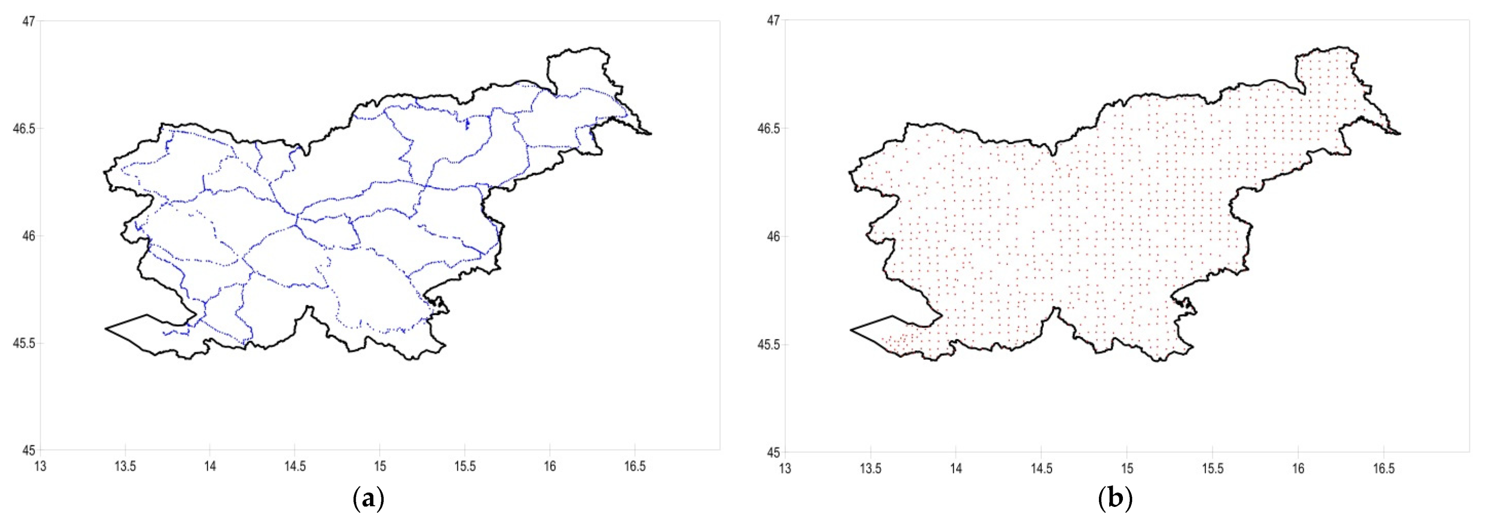
2.2. Gravimetric Data
- (A)
- Former SFRY gravimetric data covering the territory of Slovenia and part of Croatia
- (B) Data for the border area with neighboring countries (Italy, Austria, and Hungary)
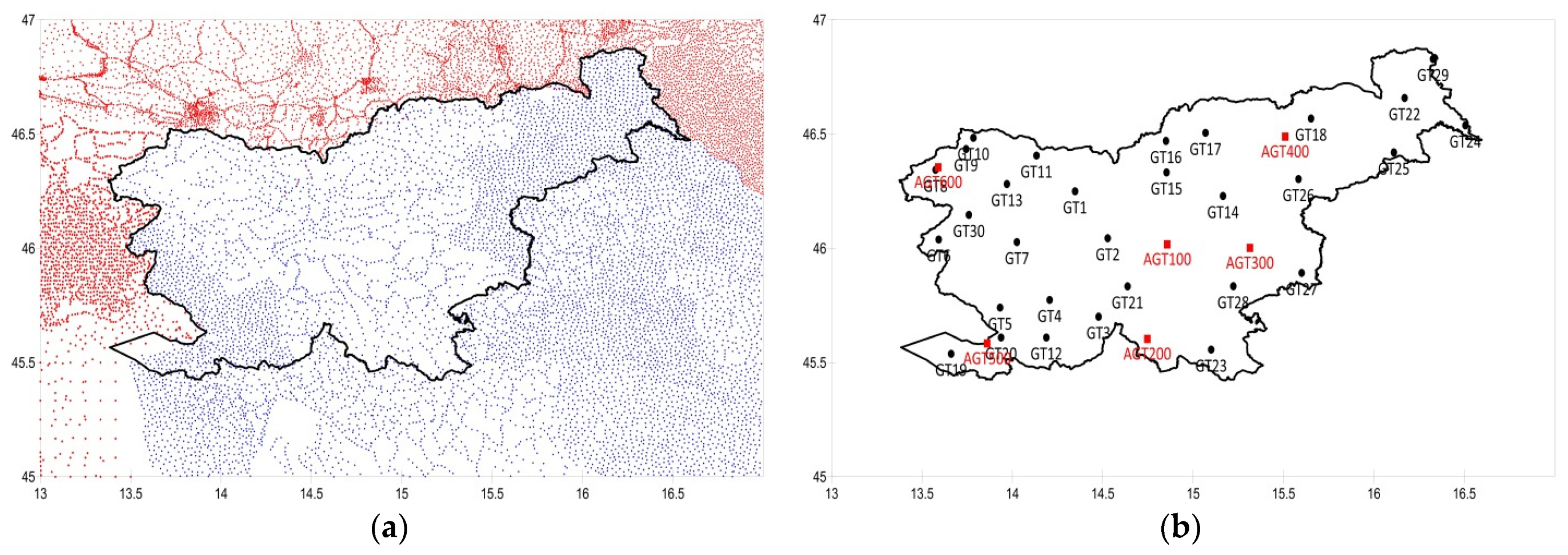
- (C) Data of the fundamental gravimetric network of Slovenia
- (D) Gravimetric data of the benchmarks of the 1st order leveling network
- (E) Data from the new regional gravimetric survey of Slovenia
2.3. Analyzing the Quality of the ‘Old’ Yugoslav Gravimetric Data
3. Methods
Calculations of the Gravity Anomalies
- Atmospheric effect [13]:
- Formula, applicable to the GRS80 ellipsoid, was used for height correction or free-air correction [13]:at which height h is expressed in meters, and the correction in [mGal].
- Topographic correction is divided into two parts: the Bouguer correction and the terrain correction.
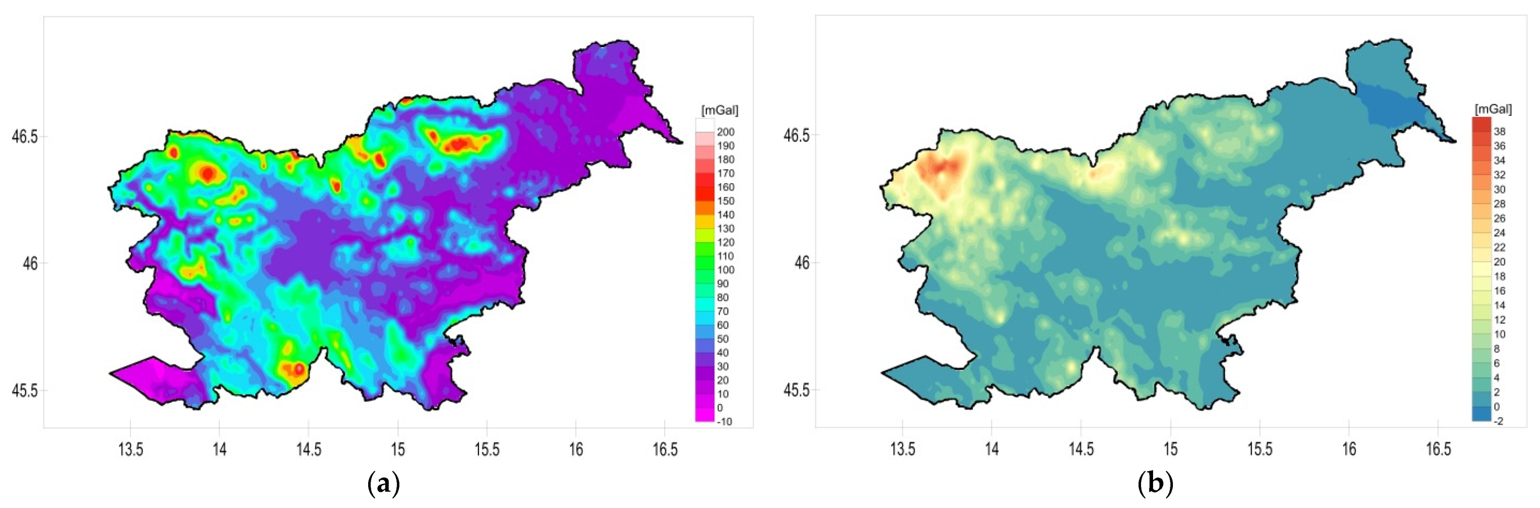
- The Bouguer correction for the points on the terrain is as follows [22,25]:where μ and λ are non-dimensional coefficients taken from [21]. A radius of 166.7 km was taken into account [25], as this is based on a sphere shaped Earth with a radius of 6371 km; G (gravitational constant) = 6.673 ± 0.01 × 1−11 m3 kg−1 s−2. This constant is a recently adopted value and differs from the value given in the GRS80 ellipsoid. h represents the reference height of the point. In the equation, the corrections are given in the unit m/s2, which is then transformed into [mGal] by multiplying it by 105, while ρ—the average Earth density—is 2670 kg/m3 [13]. Figure 7a depicts the calculated corrections for Slovenia, while the statistical indicators can be found in Table 2.
- The terrain corrections were calculated with TopoSK software [26]. The software enables the calculation of various terrain (topographic) influences or corrections of gravimetric quantities. The calculations are based on Pohanka’s formula, which calculates the gravitational effect of the polyhedral body [27], up to the distance of the outer limit of zone O (166.7 km) of the Hayford–Bowie system [28]. Different resolution DEMs, with resolution increasing toward the evaluation point, and different representations (with the option of using planar or spherical approach) of the volumetric elements are used within different integration zones of the Hayford–Bowie system. In our case, DTM25 (cell size 25 m × 25 m) was used up to a distance of 250 m, DTM100 (cell size 100 m × 100 m) from 250 m to 5240 m, and DTM1000 (cell size 1000 m × 1000 m or 3′ × 4.5′) from 5240 m on. The calculation was performed in line with the radius around each point, which was set in advance. The constant 2670 kg/m3 was adopted as the topographic density, as this should represent the average density of the rocks in the addressed area. The average value of the terrain correction was 3.03 mGal, while the standard deviation was 4.90 mGal, the minimum was 0.0 and the maximum 56.70 mGal (in Austria). The dispersion and size of the terrain corrections for the territory of Slovenia is shown in Figure 7b.
4. Results
4.1. Created Gravity Anomaly Maps
- Free air gravity anomaly:where is the observed value of the actual gravity; is the normal gravity on the GRS80 ellipsoid; is the atmospheric correction; and is the free air correction.
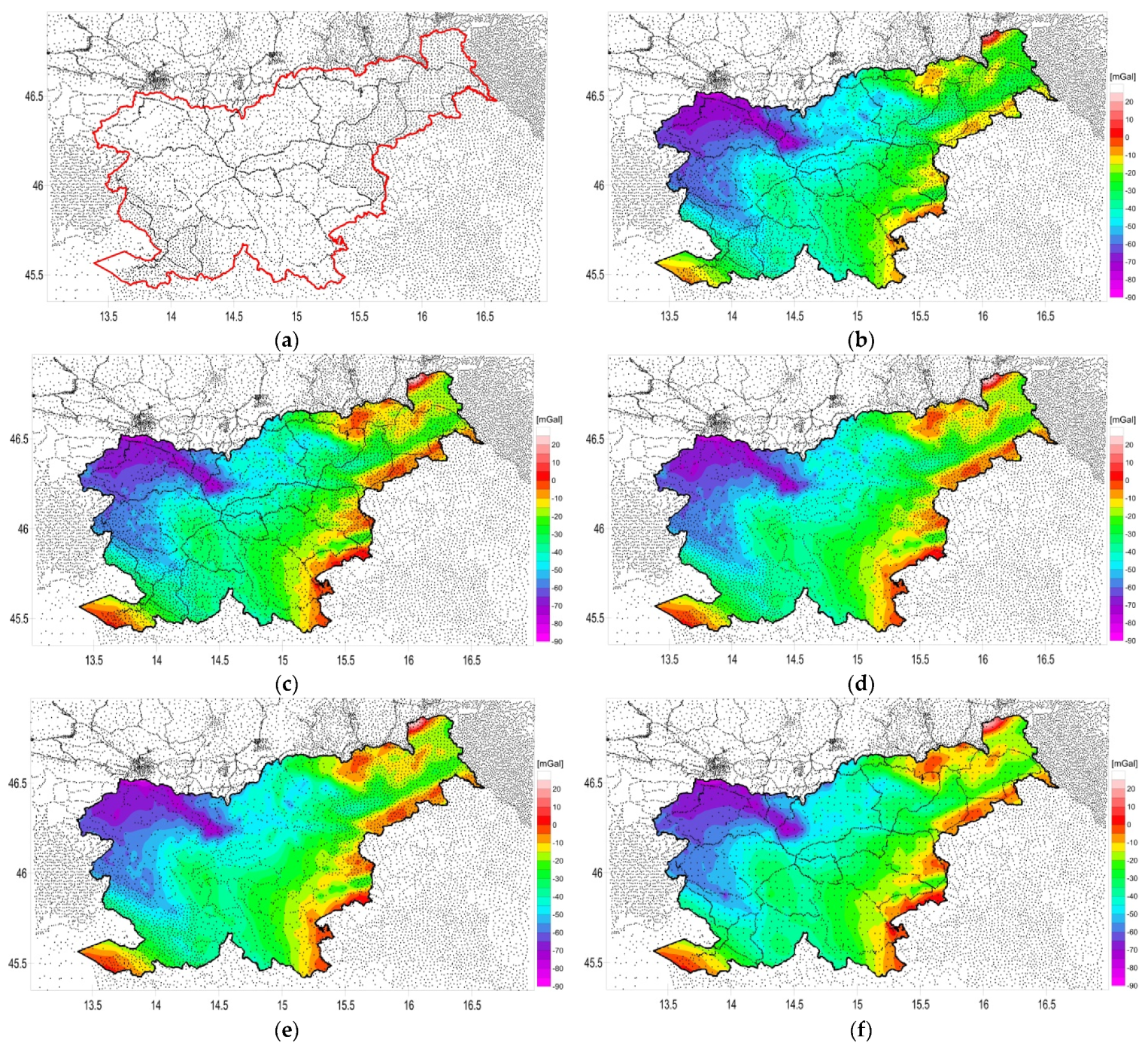
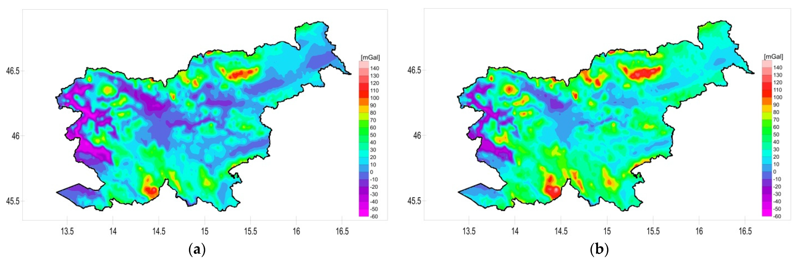
- Bouguer gravity anomaly:where is the Bouguer correction. The anomalies were calculated for all available gravimetric points and used to create the Bouguer anomaly map (SLO_BA) shown in Figure 9a.
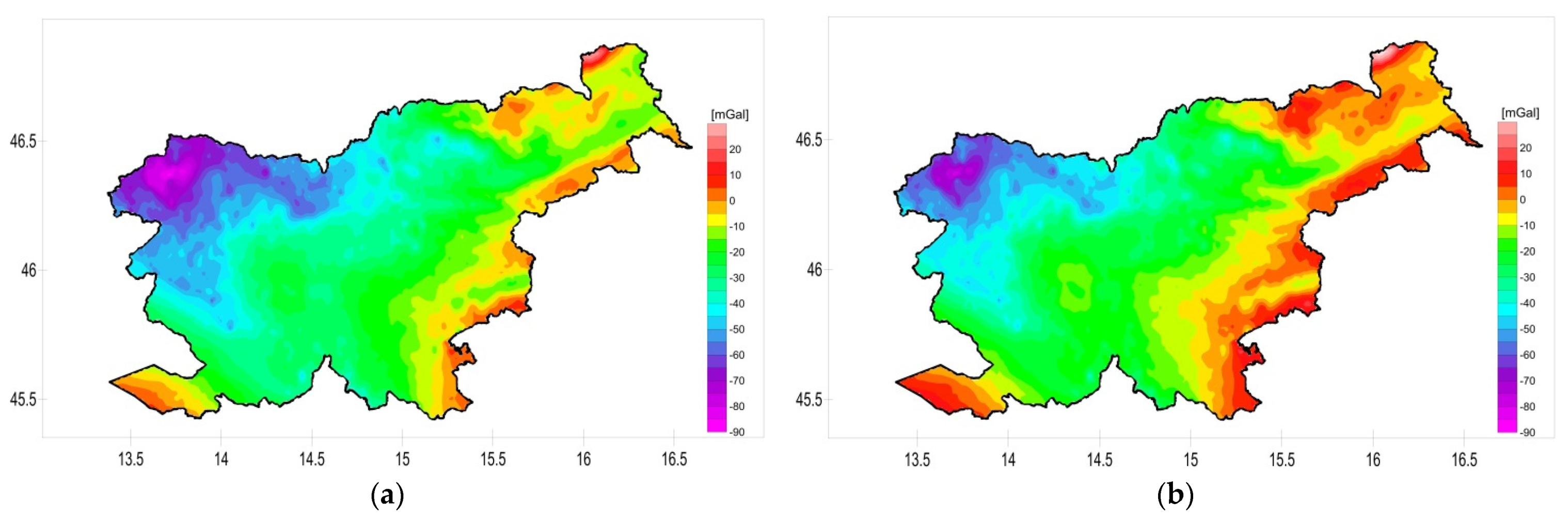
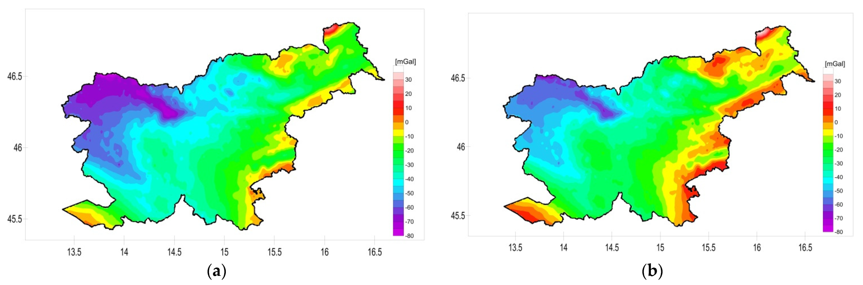
- Complete Bouguer gravity anomaly:where is the terrain correction. The complete Bouguer gravity anomaly was obtained by adding the terrain correction to the Bouguer gravity anomalies. The anomalies were calculated for all available gravimetric points and used to create the map of complete Bouguer anomalies (SLO_CBA) shown in Figure 10a.

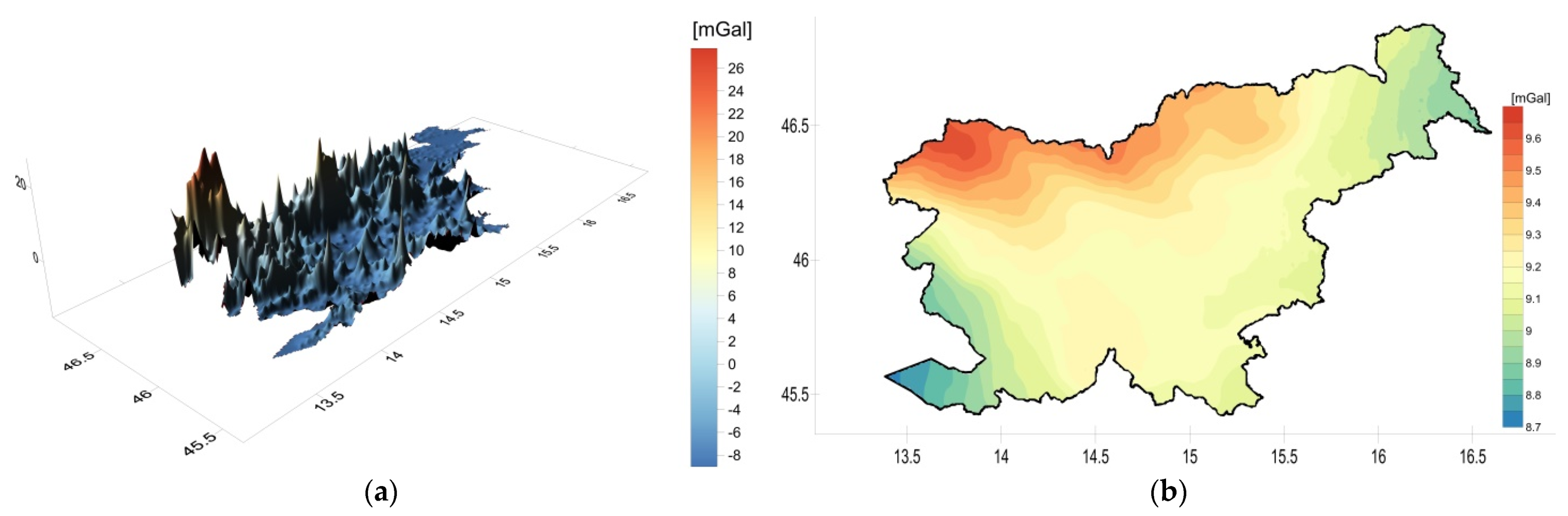
4.2. Indirect Effect
4.3. Comparison of the Gravity Anomaly Maps for Slovenia with the Analysis of the Influence of Gravimetric Data
5. Conclusions
Author Contributions
Funding
Institutional Review Board Statement
Informed Consent Statement
Data Availability Statement
Acknowledgments
Conflicts of Interest
References
- Koler, B.; Medved, K.; Kuhar, M. Projekt nove gravimetrične mreže 1. reda republike Slovenije (The Project of the New Gravimetric Network of the 1st Order of the Republic of Slovenia). Geod. Vestn. 2006, 50, 451–460. (In Slovenian) [Google Scholar]
- Bilibajkič, P.; Mladenovič, M.; Mujagič, S.; Rimac, I. Explanation for the Gravity Map of SFR Yugoslavia—Bouguer Anomalies—1:500 000; Federal Geological Institute Belgrade: Belgrade, Serbia, 1979. [Google Scholar]
- Čibej, B. Regional Gravity Map of Slovenia 1966–1967; Unpublished Report; Geological Survey of Slovenia: Ljubljana, Slovenia, 1967. (In Slovenian) [Google Scholar]
- Stopar, R. Map of the Bouguer anomalies. In Geological Atlas of Slovenia; Novak, M., Rman, N., Eds.; Geological Survey of Slovenia: Ljubljana, Slovenia, 2016; pp. 20–21. (In Slovenian) [Google Scholar]
- Gosar, A. Mohorovičić discontinuity depth. In Geological Atlas of Slovenia; Novak, M., Rman, N., Eds.; Geological Survey of Slovenia: Ljubljana, Slovenia, 2016; pp. 18–19. (In Slovenian) [Google Scholar]
- De Marchi, P.A.; Ghidella, M.E.; Tocho, C.N. Analysis of Different Methodologies to Calculate Bouguer Gravity Anomalies in the Argentine Continental Margin. Geosciences 2014, 4, 33–41. [Google Scholar]
- Meurers, B.; Ruess, D. A New Bouguer Gravity Map of Austria. Austrian J. Earth Sci. 2009, 102, 62–70. [Google Scholar]
- Kiss, J. Bouguer Anomaly Map of Hungary. Geophys. Trans. 2006, 45, 99–104. [Google Scholar]
- Tiberti, M.; Orlando, L.; Di Bucci, D.; Bernabini, M.; Parotto, M. Gravity Anomaly Map and Crustal Model of the Central-Southern Apennines (Italy). J. Geodyn. 2005, 40, 73–91. [Google Scholar] [CrossRef] [Green Version]
- Tassis, G.A.; Grigoriadis, V.; Tziavos, I.; Tsokas, G.N.; Papazachos, C.; Vasiljević, I. A New Bouguer Gravity Anomaly Field for the Adriatic Sea and its Application for the Study of the Crustal and Upper Mantle Structure. J. Geodyn. 2013, 66, 38–52. [Google Scholar] [CrossRef]
- Varga, M.; Stipčević, J. Gravity anomaly models with geophysical interpretation of the Republic of Croatia, including Adriatic and Dinarides regions. Geophys. J. Int. 2021, 226, 2189–2199. [Google Scholar]
- Zahorec, P.; Papco, J.; Pasteka, R.; Bielik, M.; Sylvain, B.; Braitenberg, C.; Ebbing, J.; Gabriel, G.; Gosar, A.; Grand, A.; et al. The First Pan-Alpine Surface-gravity Database, a Modern Compilation that Crosses Frontiers. Earth Syst. Sci. Data 2021, 13, 2165–2209. [Google Scholar] [CrossRef]
- Hinze, W.J.; Aiken, C.; Brozena, J.M.; Coakley, B.J.; Dater, D.; Flanagan, G.P.; Forsberg, R.; Hildenbrand, T.G.; Keller, G.R.; Kellogg, J.W.; et al. New Standards for Reducing Gravity Data: The North American Gravity Database. Geophysics 2005, 70, 25–32. [Google Scholar] [CrossRef]
- Farr, T.G.; Rosen, P.A.; Caro, E.; Crippen, R.; Duren, R.; Hensley, S.; Kobrick, M.; Paller, M.; Rodriguez, E.; Roth, L.; et al. The Shuttle Radar Topography Mission. Rev. Geophys. 2007, 45, RG2004. [Google Scholar] [CrossRef] [Green Version]
- Berk, S.; Komadina, Ž. Local to ETRS89 Datum Transformation for Slovenia: Triangle-Based Transformation Using Virtual Tie Points. Surv. Rev. 2013, 45, 25–34. [Google Scholar] [CrossRef]
- CRS-EU: IT_ROMA40. Available online: http://crs.bkg.bund.de/crseu/crs/eu-countrysel.php?country=IT#StartCE (accessed on 3 October 2021).
- Koler, B.; Medved, K.; Kuhar, M. The New Fundamental Gravimetric Network of Slovenia. Acta Geod. Geophys. Hung. 2012, 47, 271–286. [Google Scholar] [CrossRef]
- Medved, K.; Kuhar, M.; Stopar, B.; Koler, B. Izravnava opazovanj v osnovni gravimetrični mreži Republike Slovenije (Levelling Observations in the Fundamental Gravimetric Network of the Republic of Slovenia). Geod. Vestn. 2009, 53, 223–238. (In Slovenian) [Google Scholar]
- Koler, B.; Stopar, B.; Sterle, O.; Urbančič, T.; Medved, K. Nov slovenski višinski sistem (New Slovene Height System). Geod. Vestn. 2019, 63, 27–40. (In Slovenian) [Google Scholar] [CrossRef]
- Medved, K.; Kuhar, M.; Koler, B. Regional Gravimetric Survey of Central Slovenia. Measurement 2019, 136, 395–404. [Google Scholar] [CrossRef]
- Holom, D.I.; Oldow, J.S. Gravity Reduction Spreadsheet to Calculate the Bouguer Anomaly Using Standardized Methods and Constants. Geosphere 2007, 3, 86–90. [Google Scholar] [CrossRef]
- NGIA 2008. Gravity Stations Data Format and Anomaly Computations. National Geospatial-Intelligence Agency, Office of Geoint Sciences. Available online: https://www5.obs-mip.fr/wp-content-omp/uploads/sites/46/2017/10/computations.pdf (accessed on 11 October 2021).
- Hackney, I.R.; Featherstone, W. Geodetic Versus Geophysical Perspectives of the ‘Gravity Anomaly’. Geophys. J. Int. 2003, 154, 35–43. [Google Scholar] [CrossRef] [Green Version]
- Somigliana, C. Teoria generale del campo gravitazionale dell’ellissoide di rotazione. Mem. Soc. Astron. Ital. 1929, 4, 425. [Google Scholar]
- LaFehr, T.R. An Exact Solution for the Gravity Curvature (Bullard B) Correction. Geophysics 1991, 56, 1179–1184. [Google Scholar] [CrossRef]
- Zahorec, P.; Marušiak, I.; Mikuška, J.; Pašteka, R.; Papčo, J. Understanding the Bouguer Anomaly, Numerical Calculation of Terrain Correction within the Bouguer Anomaly Evaluation (Program Toposk); Roman Pašteka, R., Mikuška, J., Meurers, B., Eds.; Understanding the Bouguer Anomaly: A Gravimetry Puzzle; Elsevier: Amsterdam, The Netherlands, 2017; pp. 79–92. ISBN 978-0-12-812913-5. [Google Scholar]
- Pohánka, V. Optimum expression for computation of the gravity field of a homogeneous polyhedral body. Geophys. Prospect. 1988, 36, 733–751. [Google Scholar] [CrossRef]
- Hayford, J.F.; Bowie, W. The Effect of Topography and Isostatic Compensation Uponthe Intensity of Gravity; U.S. Coast and Geodetic Survey: Washington, DC, USA, 1912.
- Oliver, M.A.; Webster, R. Kriging: A method of interpolation for geographical informationsystems. Int. J. Geogr. Inf. Syst. 1990, 4, 313–332. [Google Scholar] [CrossRef]
- Nowell, D. Gravity Terrain Corrections—An Overview. J. Appl. Geophys. 1999, 42, 117–134. [Google Scholar] [CrossRef]


| Statistical Indicators | A: Set of SFRY Data | B: Set of Benchmarks | C: Set of Filtered SFRY Data |
|---|---|---|---|
| No. of points | 3364 | 2054 | 2975 |
| Min [m] | −390.94 | −22.72 | −68.65 |
| Max [m] | 333.14 | 14.45 | 68.92 |
| Mean [m] | −7.10 | 0.58 | −2.29 |
| Median [m] | −0.42 | 0.73 | −0.18 |
| St. Dev. [m] | 51.25 | 2.38 | 23.51 |
| Statistical Indicators [mGal] | SLO_NG | SLO_BC | SLO_TC |
|---|---|---|---|
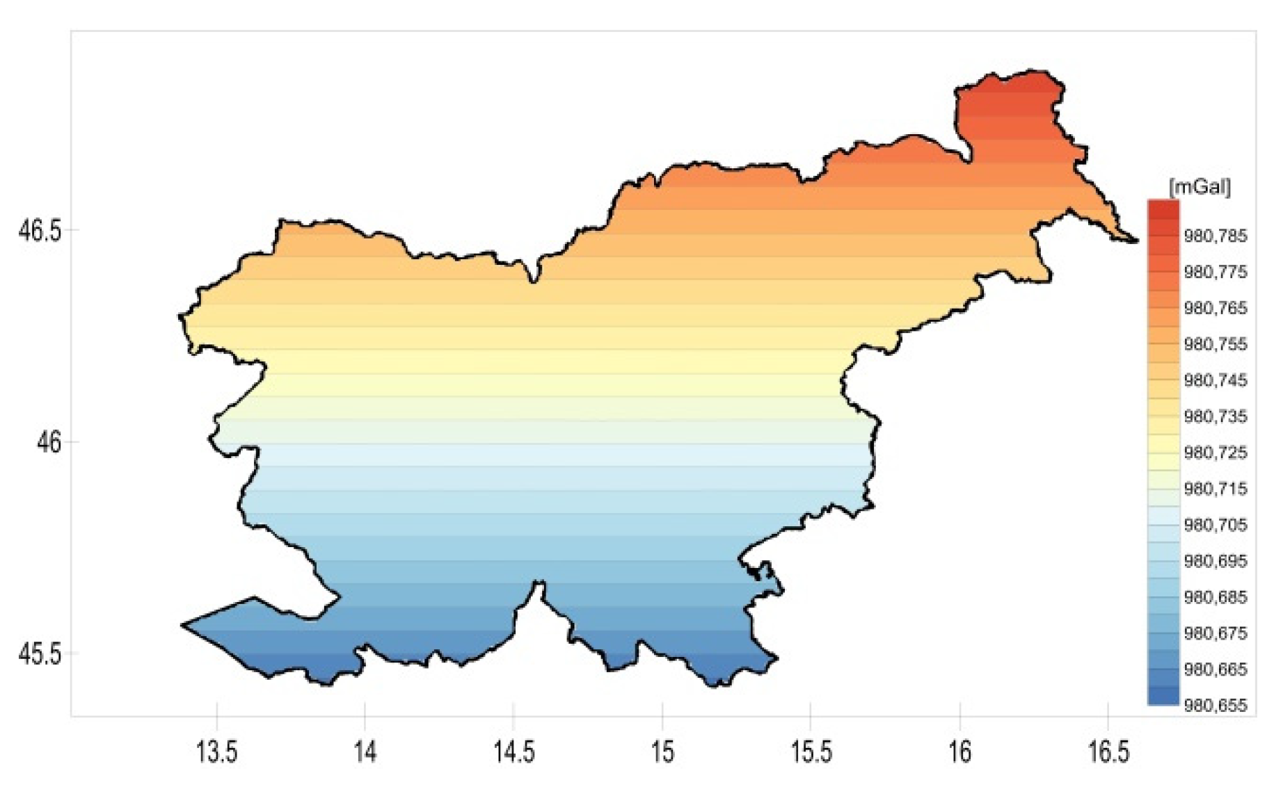
| Min | 980,658.360 | −1.680 | −0.030 |
| Max | 980,789.220 | 196.040 | 37.230 |
| Span | 130.860 | 197.720 | 37.260 |
| Mean | 980,720.731 | 55.684 | 4.185 |
| Median | 980,722.330 | 48.545 | 2.300 |
| St. Dev. | 30.591 | 31.303 | 5.173 |
| Statistical Indicators [mGal] | SLO_FAA | SLO_EFAA | SLO_BA | SLO_EBA | SLO_CBA | SLO_ECBA |
|---|---|---|---|---|---|---|
| Min | −58.620 | −44.120 | −106.030 | −96.560 | −86.620 | −77.070 |
| Max | 135.120 | 149.580 | 22.680 | 31.690 | 23.150 | 32.160 |
| Span | 193.740 | 193.700 | 128.710 | 128.250 | 109.770 | 109.230 |
| Mean | 17.878 | 32.244 | −37.806 | −28.702 | −33.621 | −24.517 |
| Median | 15.090 | 29.415 | −36.900 | −27.800 | −34.270 | −25.150 |
| St. Dev. | 26.017 | 26.078 | 21.254 | 21.142 | 17.753 | 17.652 |
| Statistical Indicators [mGal] | SLO_CBA—SLO_ECBA |
|---|---|
| Min | −9.01 |
| Max | 27.75 |
| Span | 36.760 |
| Mean | −4.918 |
| Median | −6.780 |
| St. Dev. | 5.060 |
| Difference in the Models | Min | Max | Span | Mean | Median | St. Dev | Figure |
|---|---|---|---|---|---|---|---|
| [mGal] | [mGal] | [mGal] | [mGal] | [mGal] | [mGal] | No. | |
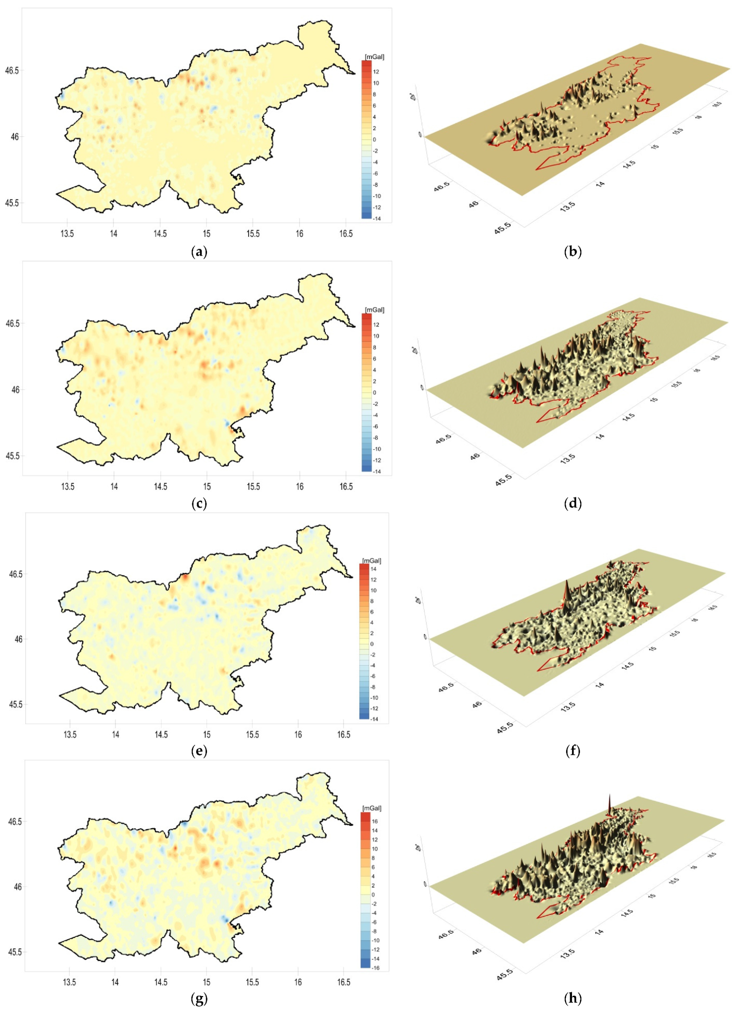
| CBA_ref—CBA_all | −12.28 | 8.42 | 20.70 | 0.02 | 0.00 | 0.42 | 13a,b |
| CBA_ref—CBA_only YU | −13.37 | 12.05 | 25.42 | 0.12 | 0.00 | 0.77 | 13c,d |
| CBA_ref—CBA_only SLO | −13.56 | 13.11 | 26.67 | −0.04 | 0.00 | 0.71 | 13e,f |
| CBA_only SLO—CBA_only YU | −15.91 | 15.24 | 31.15 | 0.16 | 0.00 | 1.10 | 13g,h |
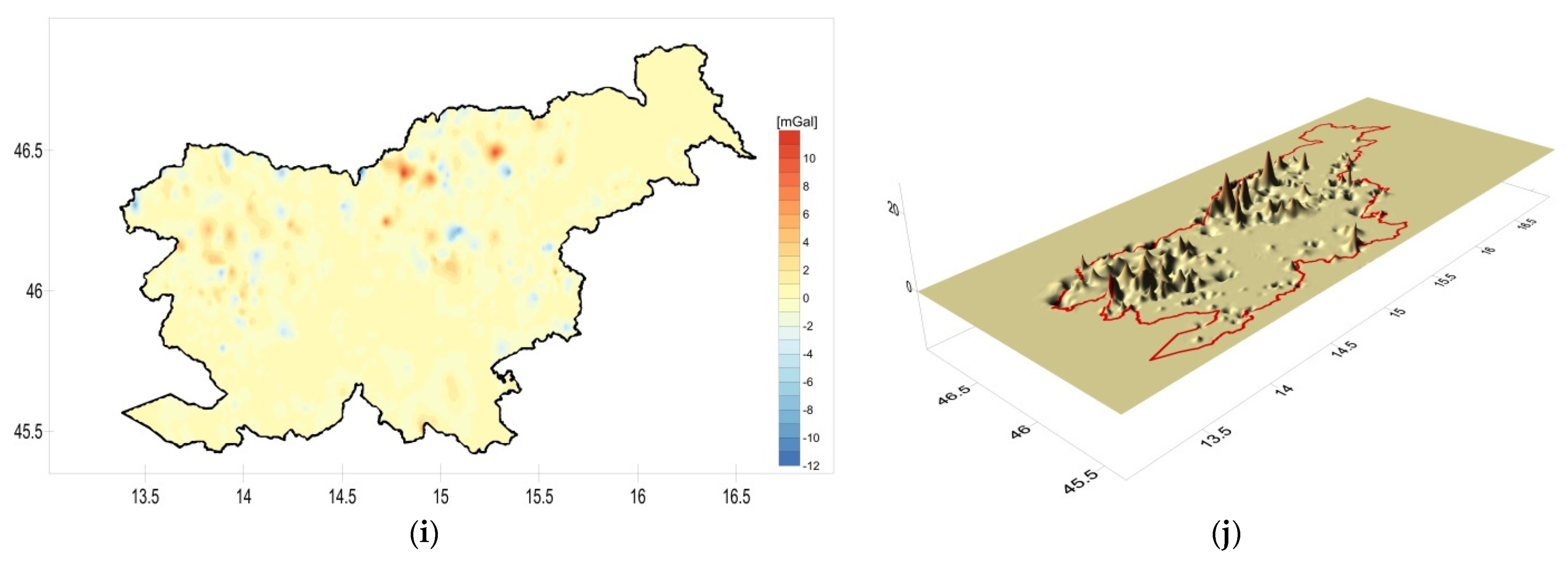
| CBA_only filter YU—CBA_only YU | −13.14 | 10.97 | 24.11 | 0.00 | 0.00 | 0.58 | 13i,j |
Publisher’s Note: MDPI stays neutral with regard to jurisdictional claims in published maps and institutional affiliations. |
© 2021 by the authors. Licensee MDPI, Basel, Switzerland. This article is an open access article distributed under the terms and conditions of the Creative Commons Attribution (CC BY) license (https://creativecommons.org/licenses/by/4.0/).
Share and Cite
Medved, K.; Odalović, O.; Koler, B. New Bouguer Anomaly Map for the Territory of the Slovenia. Remote Sens. 2021, 13, 4510. https://doi.org/10.3390/rs13224510
Medved K, Odalović O, Koler B. New Bouguer Anomaly Map for the Territory of the Slovenia. Remote Sensing. 2021; 13(22):4510. https://doi.org/10.3390/rs13224510
Chicago/Turabian StyleMedved, Klemen, Oleg Odalović, and Božo Koler. 2021. "New Bouguer Anomaly Map for the Territory of the Slovenia" Remote Sensing 13, no. 22: 4510. https://doi.org/10.3390/rs13224510
APA StyleMedved, K., Odalović, O., & Koler, B. (2021). New Bouguer Anomaly Map for the Territory of the Slovenia. Remote Sensing, 13(22), 4510. https://doi.org/10.3390/rs13224510