Abstract
Due to its dire impacts on marine life, public health, and socio-economic services, oil spills require an immediate response. Effective action starts with good knowledge of the ocean dynamics and circulation, from which Lagrangian methods derive key information on the dispersal pathways present in the contaminated region. However, precise assessments of the capacity of Lagrangian methods in real contamination cases remain rare and limited to large slicks spanning several hundreds of km. Here we address this knowledge gap and consider two medium-scale (tens of km wide) events of oil in contrasting conditions: an offshore case (East China Sea, 2018) and a recent near-coastal one (East Mediterranean, 2021). Our comparison between oil slicks and Lagrangian diagnostics derived from near-real-time velocity fields shows that the calculation of Lagrangian fronts is, in general, more robust to errors in the velocity fields and more informative on the dispersion pathways than the direct advection of a numerical tracer. The inclusion of the effect of wind is also found to be essential, being capable of suddenly breaking Lagrangian transport barriers. Finally, we show that a usually neglected Lagrangian quantity, the Lyapunov vector, can be exploited to predict the front drifting speed, and in turn, its future location over a few days, on the basis of near-real-time information alone. These results may be of special relevance in the context of next-generation altimetry missions that are expected to provide highly resolved and precise near-real-time velocity fields for both open ocean and coastal regions.
1. Introduction
Marine pollution in all its forms is a major human-induced stress on coastal and oceanic ecosystems with often dire impacts. Contaminants include nutrients [1,2], persistent organic pollutants [3], oils [4], heavy metals [5], radionuclides [6,7], and marine litter [8], such as micro and macro plastics [9,10]. By harming marine life and biodiversity, contaminants can compromise natural heritage sites, public health, and socio-economic ecosystem services, including commercial fisheries, recreation, marine aquaculture, and tourism [9,11,12]. Therefore, pollutant discharges require immediate and effective action, which starts with good knowledge of the dispersal pathways prevailing in the region where the pollution occurred.
The class of ocean physical processes that control the dispersion of a contaminated water mass depends on the spatial scale of the spill, its location, as well as the temporal window that is considered. In this work, we focus on the case of medium-size (>10 km) contamination events, typically associated with ship oil leakage, and temporal scales of days to weeks, which are the typical ones associated with a response following an oil spill event [13]. For these spatio-temporal domains, stirring by the ocean mesoscale activity is known to dominate tracer dispersal [14,15,16]. Reliable information on open ocean stirring dynamics comes from data assimilation circulation models [17] and remote sensing systems, such as satellite altimetry and high-frequency radars [18,19,20], which provide maps of surface currents. This information includes the mesoscale features present in the velocity field that are responsible for the redistribution and filamentation of any passively advected tracer down to scales larger than a few km, where submesoscale dynamics [21] and small scale turbulence eventually take over. For the case of coastal stirring processes with smaller, rapidly evolving dynamics, conventional altimetry maps are known to be less reliable, and models with data assimilation or high-frequency radars may be the only viable option.
In order to mimic the stirring process induced by mesoscale velocity fields on a contaminant and estimate its dispersal pathways, Lagrangian methods are especially useful. These methods analyze the properties of the simulated trajectory obtained by the integration of the velocity field [22]. The velocity field is then transformed into a map of the transport features that describe the spreading of a passively advected tracer (see Figure 1). Our work will focus on the Lyapunov exponent technique, a metric that tracks frontal structures controlling trajectories of passive tracers in the ocean. These structures are temporally-coherent features sometimes referred to as transport barriers [23] or Lagrangian fronts [19], and more generically belonging to the so-called Lagrangian Coherent Structures (LCS [24]). Here we will use the term “Lagrangian front”. The interest of using Lagrangian fronts to study contaminant spill dispersal or when tracking a specific water mass during an in situ campaign study is obvious: as the front moves, it attracts and stretches the tracers along its pathway. At the same time, it acts as a transport barrier inhibiting the cross-frontal dispersal of the tracers (Figure 1).
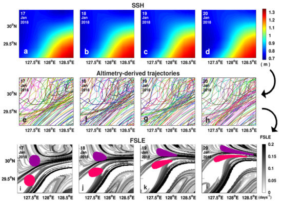
Figure 1.
Sketch of a Lagrangian analysis applied to a velocity field (in this case, altimetry-derived geostrophic velocities). Panels (a–d) correspond to altimetry maps highlighting the daily sea surface heights from the 17th to 20th of January 2018 in a frontal area near the region of the East China Sea accident. The first step leading to the calculation of a Lyapunov field is the computation of backward Lagrangian trajectories depicted in panels (e–h). Panels (i–l) show the finite-size Lyapunov exponent in the same area, identifying oceanic Lagrangian fronts. The daily shape deformation of two passive tracers (in purple and fuchsia) due to a nearby Lyapunov front (black filament) is added as an illustration.
The use of Lagrangian methods has received considerable attention in many problems related to tracer dispersal, including phytoplankton dynamics [25]. It has also been proposed as an operational tool for cases of pollutant dispersion. However, little attention has been paid to the evaluation of the efficiency of these Lagrangian methods in real cases of contaminant dispersion, such as oil spill accidents. An exception is the DeepWater Horizon oil spill, which occurred in the Gulf of Mexico in April 2010 while drilling near the mouth of the Mississippi River, and is reported to be the largest accidental marine oil spill in the history of the petroleum industry. Lagrangian studies were performed on this oil spill by Olascoaga and Haller (2012) [26]. Duran et al. (2018) [27] also showed statistical consistency between climatological LCS and the DeepWater Horizon spill trajectory. Using such a massive spill for Lagrangian validation studies has the advantage that the smaller circulation scales, not necessarily well resolved by the velocity fields, play a secondary role over the effect of larger eddies and jets in the vast surface areas occupied by the spill. Nevertheless, massive contaminations are rare compared to accidents that may involve individual ships or short-time spills. Is the Lagrangian approach also reliable for smaller accidents? In this paper, we considered two real cases of accidents: an offshore oil spill that occurred in the East China Sea in 2018 and one event of coastal oil pollution in the eastern Mediterranean Basin in 2021.
As a main goal, this paper attempts to use Lagrangian information to analyze these two oil spill cases while qualifying the efficiency of satellite altimetry and data assimilation models in each of the accidents. By doing this, this paper also shows that a usually neglected Lagrangian quantity, the Lyapunov vector, contains, in fact, precious information for managing contaminant accidents because it informs on the drifting velocity of the tracer patch contained by Lagrangian fronts.
This article is structured in the following way. In Section 2, satellite and model data are described, followed by a presentation of the Lagrangian techniques. These include the finite-size Lyapunov exponent (FSLE), one of the main tools used to detect Lagrangian fronts in near-real-time oil spill analysis and pollution management. Near-real-time analysis of pollution spreading, such as oil spills, ideally requires additional information on the future displacement of the Lagrangian fronts controlling the contaminant dispersion. Therefore, Section 2 also contains a heuristic method using the Lyapunov vector to make a short-term prediction of the Lagrangian fronts’ drifting over a few days, without the need for future predicted velocity fields. Section 3 and Section 4 examine and discuss the results of the Lagrangian techniques for each of the two pollution cases while considering the direct wind impact on the transport pathways. The conclusions and perspectives are drawn in the final section.
2. Materials and Methods
2.1. The East China Sea Oil Spill
The first case study is an oil spill accident that occurred in the East China Sea (ECS) after a collision on the 6th of January 2018 (30°51.1′N, 124°57.6′E) between the Hong Kong-flagged cargo ship CF Crystal and the Iranian oil tanker Sanchi, carrying hundreds of thousands of metric tons of a full natural-gas condensate (ultra-light crude) cargo [28,29,30]. On the 14th of January 2018, the Sanchi oil tanker exploded after burning for more than one week and sank at the location (28°22′N, 125°55′E) [28,29,31]. We will refer, in the following, to this accident as the “East China Sea oil spill”.
This case is well suited for an analysis focused on the effect of horizontal stirring. Over the spatiotemporal scales of the East China Sea oil patch (10–100 km) and the duration of the accident (several days), the mesoscale circulation active in the region redistributed the contaminated water in a complex pattern [29]. Such a mesoscale activity is organized by the Kuroshio Current (Figure 2), a major western boundary current that sheds energetic eddies and creates a region of strong strain around its core [29,31,32]. In particular, panels (a,c,d) highlight the presence of a strong frontal oceanic structure associated with the Kuroshio Current.

Figure 2.
The region of the oil spill accident in the East China Sea, in the Northwest Pacific ocean. Panels (a,b) illustrate the 2018 mean sea surface height (in m) and the 2018 mean eddy kinetic energy (in cm2/s2), respectively. The white rectangle shows the East China sea oil spill area that is reported in panels (c,d). The sea surface heights (color, in m) and the derived current velocities (arrows, in m/s) in the smaller scaled region of the East China Sea oil spill on the 18th of January 2018 are mapped in panel (c). The altimetry-derived finite-size Lyapunov exponent (in days−1) for the same date is computed backward in time (d).
2.2. The East Mediterranean Oil Spill
The second case study we analyzed occurred in the Mediterranean Sea in February 2021, when Levantine countries witnessed the arrival of oil pollutants, particularly tar-balls, washing up onshore. The origin of the pollution is unclear. It might be oil leaked from a ship or illegally dumped into the water from a tanker. The vessel responsible for such a disaster is still unidentified as many vessels were near the location (50 km offshore from the Lebanese coast). On the 12th and 13th of February 2021, two slicks of oil were detected near the shore (~30 Km from the coast) in the southeast Levantine basin from SAR images. We will refer to this second case study as the “East Mediterranean oil spill”.
The Mediterranean Sea (Figure 3) is a highly active Atlantic-Suez shipping corridor and hosts about 10% of the global shipping activity. It is subjected to frequent oil spills and discharges from ships [33,34]. Confronting such threats in the semi-enclosed Mediterranean Sea is crucial as they put the marine ecosystems at risk. The Mediterranean Sea is, indeed, rich in biodiversity with a high rate of endemism and contains 4% to 18% of the global marine biodiversity [35]. Cleaning up these types of oil spills would take months or years, with negative socio-economic impacts on tourism, health, and fishing.
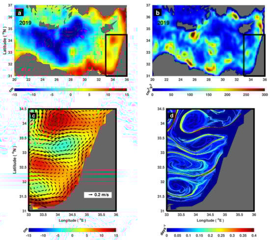
Figure 3.
The region of the oil spill accident in the Mediterranean Sea. Panels (a,b) represent 2019 mean sea surface height (in cm) and the mean eddy kinetic energy (in cm2/s2), respectively, in the Eastern Mediterranean basin. The black rectangle shows the region affected by the East Mediterranean oil spill, which is reported in panels (c,d). The sea surface height (color, in cm) and the derived current velocities (arrows, in m/s) in the smaller scaled region of the East Mediterranean oil spill on the 2nd of July 2019 are mapped in panel (c). The altimetry-derived finite-size Lyapunov exponent (in days−1) for the same date is computed backward in time (d).
2.3. Oil Slick Detection
SAR has proven to be a very valuable technique for tracking and monitoring surface oil pollution, whether occurring offshore in the open ocean or in coastal water, undisturbed by the land thanks to its high resolution (up to ~10 m). A typical SAR image of the ocean appears as a dark image with some gray or white slicks. A floating oil slick weakens the surface roughness that is usually engendered by what is known as short gravity-capillary waves (see Marangoni theory detailed in Marangoni (1871) [36] and Alpers and Hühnerfuss (1988) [37]). The short gravity-capillary waves and the inferred surface roughness are responsible for the radar back-scattering that triggers grayish-white patches on SAR images of the sea surface. However, when the waves are damped by the surface oil, dark patches are visualized on the SAR images. This is the principle of detecting the oil slicks on the ocean surface by SAR-equipped satellites. Nevertheless, dark patches on SAR images of the sea surface can also result from a phytoplanktonic bloom, the turbulence engendered by a ship propeller, and any other phenomenon capable of damping the short gravity-capillary waves, thus reducing the back-scattered radar power. To avoid ambiguity and optimize the detection of surface oil slicks by SAR images, with the highest contrast among slicks, several parameters should be taken into account. These include radar configuration, slick nature, and meteorological and oceanic conditions. These are detailed in Chapter 11 in Jackson et al. (2004) [38] and Girard-Ardhuin et al. (2005) [39].
Remotely sensed observations of the East China Sea oil trajectory and the East Mediterranean oil slicks were analyzed by the “Collecte Localisation Satellites” company (CLS) in Brest. The oil patches were detected using Terrasar, Sentinel1, Sentinel2, and Sentinel3 Imagery. Contours of the East China Sea oil spill have been manually detected from these images for the period from the 17th to 20th of January 2018 (see Figure 4). The East Mediterranean contamination was revealed as a set of disconnected patches of variable size observed at the surface. Here, we focused on the two largest slicks that were tracked near-shore in the southeastern Levantine basin on the 12th of February 2021.
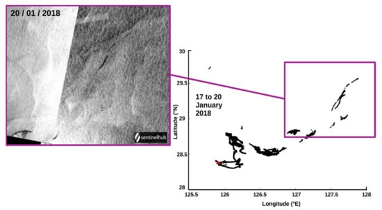
Figure 4.
East China Sea oil spill trajectory from the 17th to 20th of January 2018 detected by SAR images.
2.4. Satellite Observations and Numerical Models
All the data involved in the Lagrangian applications are provided by Copernicus Marine Environment Monitoring Service (CMEMS, http://marine.copernicus.eu/services-portfolio/access-to-products, accessed on 15 June 2021). Different products of current velocities were used with particular attention to near-real-time datasets as they are usually the only products available when unexpected accidents occur.
2.4.1. Global Current Velocities
Surface geostrophic currents in near-real-time (NRT) are derived from the sea surface height above geoid (SSH) and are provided by a global satellite product (product id: SEALEVEL_GLO_PHY_L4_NRT_OBSERVATIONS_008_046) processed by the DUACS multimission altimeter data processing system. This product treats data from all available altimeter missions: Jason-3, Sentinel-3A, HY-2A, Saral/AltiKa, Cryosat-2, Jason-2, Jason-1, T/P, ENVISAT, GFO, and ERS1/2. Daily surface observations of the global ocean were chosen with L4 processing level and a spatial resolution of 0.25° × 0.25°. We also used altimetric currents in a delayed-time version with L4 processing level (id: SEALEVEL_GLO_PHY_L4_REP_OBSERVATIONS_008_047), providing daily estimations of the sea surface heights above the geoid and the derived surface geostrophic currents with a spatial resolution of 0.25° × 0.25°. We also employed the CMEMS NRT geostrophic velocity fields, including a modeled Ekman current based on ECMWF NRT winds (product id: MULTIOBS_GLO_PHY_NRT_015_003). Daily mean global ocean currents were used in this work with 0.25° × 0.25° spatial resolution and L4 processing level. This product was chosen to estimate the wind impact on the ocean current, which, in turn, could affect the transport of contaminants. Aside from remotely sensed data, we tested ocean surface velocity data from the Mercator global ocean analysis and forecast system, providing a 3D daily analysis (product id: GLOBAL_ANALYSIS_FORECAST_PHY_001_024). This numerical model assimilates different parameters, including sea level, sea ice concentration and thickness, in situ TS profiles, and sea surface temperature (SST) over 50 depth layers. Here we considered the daily analysis-derived current velocities at the surface, in near-real-time, with 0.083° × 0.083° spatial resolution and L4 processing level.
2.4.2. Mediterranean Current Velocities
For the Mediterranean application, we started by identifying the near-real-time Lagrangian fronts using the regional European Seas daily altimetric geostrophic velocities with 0.125° × 0.125° horizontal resolution (product id: SEALEVEL_EUR_PHY_L4_NRT_OBSERVATIONS_008_060). The Lagrangian analysis was then repeated using near-real-time model analysis data with a higher horizontal resolution (0.042° × 0.042°) provided by a coupled hydrodynamic-wave model implemented over the whole Mediterranean Basin, by the Mediterranean Forecasting System (MFS) (product id: MEDSEA_ANALYSISFORECAST_PHY_006_013).
2.4.3. Surface Wind Velocities and Current-Wind Mixed Product
According to NOAA (2002), the oil pathway is not only subjected to the current velocities but can also be affected by other factors, including the direct wind forcing. For this purpose, we created a new velocity product where we added 3% windage (the average value recommended by NOAA) to the current velocities. Although not all the results were presented in the paper, the Lagrangian analyses were repeated with and without this direct wind forcing to evaluate the impact that it could have on the results. We used daily means of surface wind speed from the IFREMER CERSAT Global Blended Mean Wind Fields with 0.25° × 0.25° spatial resolution and L4 processing level (product id: WIND_GLO_WIND_L4_NRT_OBSERVATIONS_012_004).
2.5. Lagrangian Advection and Derived Trajectories
In order to generate particle trajectories, the current velocity fields described above were linearly interpolated in time (with a step of 3 h) and space (at the exact position of each point along a trajectory). The integration in time of the velocity field was performed with a Runge–Kutta integrator of the fourth-order [25]. A detailed description of this method is found in reference [40].
For the East China Sea oil spill case, we started by a 6-day advection of a numerical tracer (radius 0.3° (~33 Km)) centered at the location of the East China Sea and representing the initial oil patch. The starting date is the 14th of January 2018, the day when the oil slicks were observed at the surface for the first time. The chosen duration of advection (6 days) reflects the fact that the last day’s available data for East China Sea oil slicks were those of the 20th of January 2018. A numerical experiment of direct advection was performed only for the East China Sea oil spill whose origin location was well-known, unlike that of the East Mediterranean pollution.
2.6. Lagrangian Fronts Detection by the Lyapunov Exponent
We estimated Lagrangian fronts as ridges in a map of both finite-time (FTLE) and finite-size (FSLE) Lyapunov exponents [19,23,41,42,43].
The finite-size Lyapunov exponent (λ) is defined by the following equation:
where d0 represents the initial size of a water parcel at time t0, and τ the time needed to reach a maximal stretching length of df.
λ not only depends on d0 and df but also on the initial position of the particle pair x0 and the time of deployment t0. For both FTLEs and FSLEs the calculation was done with four equally spaced particles at fixed distance d0 from a central particle located at x0, and then advanced after diagonalizing the Cauchy–Green tensor formed by the evolution in time of these particles [44].
The finite-time and finite-size Lyapunov exponent calculation [23,42,45,46,47] are two Lagrangian methods that analyze the rate of deformation that a water parcel undergoes while being advected. For geophysical flows, the limit for integration time is relaxed to a finite temporal window, which is set explicitly for the finite time calculation. For the case of the finite-size Lyapunov exponent, the integration ends when a finite perturbation of a fixed size reaches a prescribed final growth.
Lyapunov exponent maps can localize in space and time geometrical features that are relevant for the tracer transport. Examples of geophysical applications are many, for both the atmosphere [45,46,48] and the ocean [42,49,50,51,52].
When computed backward in time on a two-dimensional geophysical flow, a spatial map of Lyapunov exponents typically presents some ridges that can be interpreted as Lagrangian fronts. The value of a Lyapunov exponent has units of the inverse of time and indicates the rate of confluence, that is, the exponential decrease of the distance between two water parcels during their advection towards the confluence region. A tracer released nearby a ridge of high Lyapunov exponents is attracted by this line exponentially fast. Under an approximation of small divergence/convergence, the compression of the distance between two water parcels must be compensated by stretching in the orthogonal direction. As a consequence, a ridge of maximal Lyapunov exponents is also a line along which a tracer (for instance, a contaminant) is stretched into a filament.
2.7. Estimating the Drifting Speed of a Lagrangian Front
An original development of our work is a method for predicting the drifting speed of a Lagrangian front. We described this new method here and then applied it in the Results Section. Panels (i–l) of Figure 1 illustrate that a Lagrangian front has several interests in the case of a contaminant spill: it attracts the contaminant, it stretches it, and at the same time, it contains the tracer, acting as a transport barrier. Therefore, knowing the position of Lagrangian fronts in a region where a contaminant spill has occurred helps in estimating the shape that the contaminated water will assume on timescales of the order of the inverse of the Lyapunov exponent value [26].
The exponential dynamics of a tracer undergoing stretching over the front typically occurs much faster than the drift of the front itself. For this reason, the Lagrangian front is often approximated as stationary [26]. Nevertheless, Lagrangian fronts do evolve in time [26] (see Figure 5). The possibility of anticipating the future front position and its folding has an obvious interest when estimating the fate of a pollutant, as well as for characterizing the dynamics of frontogenetic processes across the ocean basins [23,24,42,53].
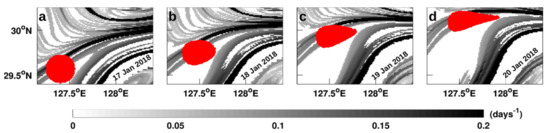
Figure 5.
A moving Lagrangian front simultaneously transporting a nearby numerical tracer. Panels (a–d) are daily finite-size Lyapunov exponent maps from the 17th to 20th of January 2018. The sharpest Lagrangian front attracts the red numerical tracer and at the same time displaces the tracer northward while drifting in this direction. The drift of the front occurs during the stretching of the passive tracer. Without considering the drift of the front, the predicted position of the tracer would be expected several tens of km south of its real position.
How can the drifting speed of a Lagrangian front be estimated? Our starting point to answer this question is a theoretical property of the flux across Lagrangian fronts found by Shadden et al. (2005) [54] (later corrected by Haller et al. (2011) [55] by adding missing assumptions). These authors considered Lagrangian fronts defined as ridges of finite-time Lyapunov fields. They showed that under general conditions, this flux can be considered “small, and in most cases negligible for well-defined LCSs or those where the rotation speed is comparable to the local Eulerian velocity field, and can be computed from FTLE fields with a sufficiently long integration time” [54] (p. 271). Haller et al. (2011) [55] added further assumptions so that the long integration time conditioning a negligible across-front flux, according to Shadden et al., remains valid.
Although the objective of Shadden et al. was to provide a firm mathematical ground to the interpretation of ridges of Lyapunov exponents as transport barriers, the condition of minimal flux across a ridge of a Lyapunov field could also be used to estimate the drifting speed of the ridge itself. Consider the case in which the flux across that Lagrangian front was strictly equal to zero, or at least small enough so that the drifting speed of the front can be approximated by the zero-flux case. In this case, whenever a ridge appears to be transverse to a smooth velocity field (see Figure 6A), a sufficient condition for maintaining a zero flux is to impose a local displacement of the ridge by the component of the velocity field orthogonal to the ridge (Figure 6B,C).

Figure 6.
A sketch resuming the method used for the short-term prediction of front drifting presented in this paper. Panel (A) represents the starting position of a water mass (filled blue patch). Panel (A,C) show the new position of the same water mass (filled blue patch) after a few days. The old position is reported as a hashed circle. Assuming that the water flux is negligible across a Lagrangian front (black line in panel (A)), the front should move as the water particle drifts with a speed (purple arrow) directed across and orthogonal to the front. Otherwise, the water particle crosses the filament, which will no longer be considered as a well-defined front or transport barrier (panel (B) and the associated FSLE map). The front drifting speed is represented by the purple arrow in panel (C) in which the dashed line defines the initial position of the front before its movement. The continuous black arrow in all panels corresponds to the altimetry-derived velocity vector. Panels are accompanied by examples of FSLE showing the need for the front to drift in order to conserve its characteristic as a transport barrier. By drifting, the front prevents the cross-frontal passage of the blue water mass, as shown in the FSLE map accompanying panel (C).
2.8. Sea Surface Temperature
We used daily global satellite observations of near-real-time sea surface temperature with 0.05° × 0.05° horizontal grid resolution and L4 processing level. The product provides a gap-free map generated by the Operational Sea Surface Temperature and Ice Analysis (OSTIA) system using in situ and satellite data from infrared and microwave radiometers. The SST product is also available by CMEMS with the following id: SST_GLO_SST_L4_NRT_OBSERVATIONS_010_001.
3. Results
3.1. Lagrangian Advection of Virtual Numerical Tracer vs. East China Sea Oil Imaging
The first case we considered was the East China Sea oil spill. The first experiment we performed was a direct advection of a passive tracer released at the accident location using different velocity fields. In Figure 7a–d, the resulting advected trajectories using the different velocity products were mapped in red. They were compared to the East China Sea oil propagation detected from SAR images, plotted in black. When using the delayed-time and near-real-time data from the 14th to the 20th of January 2018 (Figure 7a,b), the advected pattern was incompatible with the real trajectory of the East China Sea spill. Indeed, the stretching observed in the oil path on the 20th of January 2018 (Figure 4 and north-eastern part of the study region) was not detected by the simple altimetric advection method in both panels. To take into account the wind impact on the current transporting the oil, we repeated the 6-day advection experience using the geostrophic velocity fields combined with modeled Ekman current. According to Figure 7c, the addition of the wind impact did not improve the results nor affect the conclusions. Another 6-day advection was then made using the Mercator analysis product in Figure 7d. Although the resulting advection seemed to be more reliable in terms of strain and northeastward direction, the actual trajectory lay south of the advected one, which remains insufficient for the analysis of such oil spill pathways. The advection experiment was also repeated by adding the 3% windage to consider the direct wind impact on the oil itself (NOAA, 2002). Very little change was noted, and not surprisingly, due to the weak wind intensity (<7 m/s, results not shown).
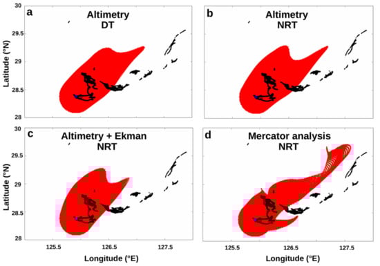
Figure 7.
Six-day advection of a numerical tracer corresponding to East China Sea oil spill using different current velocity products (from satellite observations and the Mercator numerical model). The red patterns in panels (a–d) correspond to the output trajectory after a 6-day advection since the 14th of January 2018, initializing the tracer at the oil spill site. In panel (a), the red trajectory is computed from delayed-time altimetry, and in panel (b) from near-real-time altimetry. In panel (c), the red trajectory is computed from near-real-time altimetry combined with Ekman currents, and in panel (d) from Mercator analysis surface velocities. The real oil pathway is mapped in black based on satellite image analyses. The blue asterisk represents the location where the Sanchi tanker sank.
3.2. Regional Application of Lagrangian Fronts on East China Sea Pollution: Offshore Dynamics
We then identified Lagrangian FSLE fronts in the location of the East China Sea oil spill accident using the near-real-time surface geostrophic velocities (Figure 8). Note that the cross-frontal drift will be examined in Section 3.4.1. The red patch represents the daily trajectory of the leaked oil available from the 17th to the 20th of January 2018. As observed in Figure 8, the daily shape and displacement of the East China Sea oil spill were remarkably consistent with the location and shape of the fronts underlined by the FSLE map. The most intense front highlighted on the 17th of January became sharper in the following days, and it presented a stretching zone attracting the oil tracer. The oil spill rapidly extended along the front direction, as seen on the 20th of January 2018. This sharp front evidenced the Kuroshio Current impact in the spill location, capable of transporting the pollution over large distances and in a short amount of time [29,32].
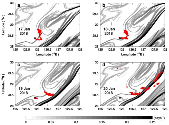
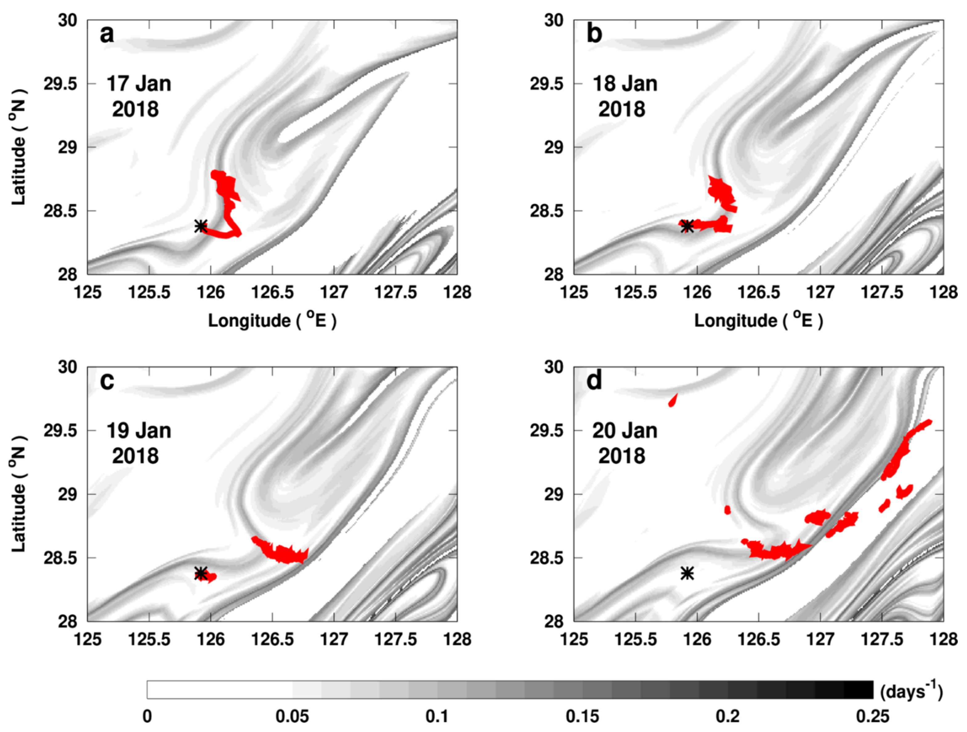
Figure 8.
Daily backward finite-size Lyapunov exponent (FSLE) in the East China Sea oil spill region. The black asterisk in all panels indicates the location where the Sanchi tanker sank. The red patch represents the daily evolution of the leaked oil patch (observed from satellite images) from 17th to 20th of January 2018 in panels (a–d), respectively. The gray-scaled filament-shaped fronts in the background represent daily Lagrangian fronts (FSLE computation). Black fronts reveal highly attractive and stretching zones. In this case, the sharpest front is related to the core of the Kuroshio Current.
The same experience was repeated using (i) the velocity-derived altimetry product in delayed-time instead of near-real-time (Figure A1); (ii) the velocity product with added Ekman impact (Figure A2); and (iii) analysis-derived velocities in near-real-time provided by the Mercator global ocean analysis and forecast system (Figure A3). For (i) and (ii) cases especially, the results were similar with no significant additional information. Backward FSLE based on Mercator product provided a much more complex distribution of Lagrangian fronts, with more features and finer scale information than altimetry-based calculations. However, the additional details were not confirmed by similar patterns in the oil patch. Moreover, the higher number of smaller Lagrangian fronts rendered it more complicated to distinguish which one would control the spilled oil. There was no real improvement to the positions given by the simple use of observational altimetry.
For the offshore East China Sea spill, and consistently with the direct advection experiment, the addition of wind drag, through the use of the mixed current-wind velocities (see Section 2.4.3), did not improve the results (results not shown).
3.3. Regional Application of Lagrangian Fronts on the East Mediterranean Pollution: Coastal Dynamics and Strong Wind
On the 12th of February 2021, two oil slicks were spotted near the shore in the southeastern Mediterranean basin in SAR images (see Figure 9). We started by a Lyapunov exponent computation in the polluted area in the southeast of the Levantine basin, using the altimetry-derived current velocities. In this coastal region, altimetry seemed insufficient for the detection of near-shore fronts where the spilled oil was observed (the red slicks in Figure 9c). This is not surprising, as one limitation for satellite altimeters is their inaccuracy near the land shore (at least 5–10 km from the coast) that increases in regions of small Rossby radius such as in the Mediterranean [55,56,57,58,59].
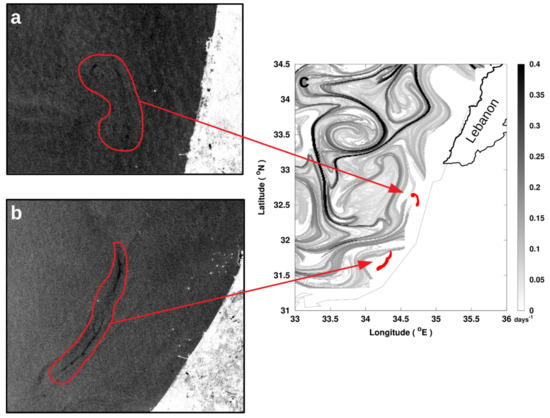
Figure 9.
Altimetry-derived FSLE map of the 12th of February 2021, with the corresponding oil slicks detected by SAR images. (a,b) are the SAR images for two slicks of oil identified near the coast on the 12th of February provided by Sentinel-1. The FSLE map in (c) highlights the Lagrangian fronts in near-real-time in the southeastern Levantine basin, with the oil trajectories mapped in red.
For a more reliable near-shore analysis in the southeastern Mediterranean basin, we chose the data assimilating model analysis from the Mediterranean Forecast System (MFS). The model allowed the tracking of an along-shore Lagrangian front trapping the oil on the 12th of February, thus explaining the shape of both pollutants, the northern and southern ones (see Figure 10b). Indeed, there was a consistency between the front direction and the form of the two oil slicks. The southern part was stirred along the front, while the northern one seemed to curve following the front curvature (see Figure 10b). The model-derived front could not be tracked using altimetry alone (see Figure 10a). According to the SAR images, the two oil slicks observed on the 12th of February persisted to the next day while still in contact with the same front.
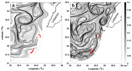
Figure 10.
Comparison between Lagrangian fronts (gray) (a) derived from altimetry and (b) derived from the Mediterranean circulation model. The red patterns in (a,b) represent the position of the oil slicks on the 12th of February 2021.
The Lyapunov experiment was repeated for the 12th and 13th of February using a 3% windage component included in the mixed current-wind product (NOAA, 2002). The resulting fronts are shown in Figure 11a,b. On both days, the Lagrangian front responsible for the oil retention was still well-detected when adding the windage, but with minor impact on the front retaining the northern oil slick (32.6°N, 34.7°E), as seen in Figure 11a. Nevertheless, there was an intensification of the wind speeds starting on the 16th of February (see Figure 12), which persisted for a few days with a pronounced eastward direction. Simultaneously, the gray-scaled fronts inferred from the mixed current-wind product drifted to the east, as if the wind was shifting all of the local fronts following its direction. Such phenomena could have accelerated and facilitated the arrival of oil onto the eastern Levantine coasts.
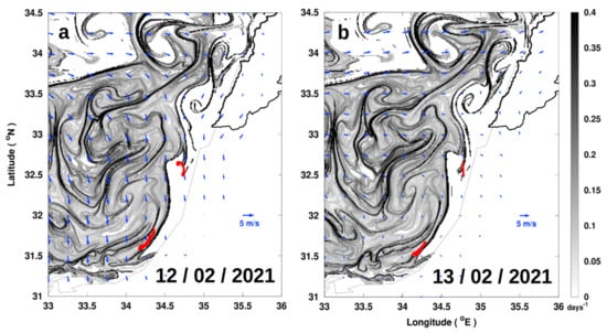
Figure 11.
FSLE maps using surface currents corrected with a wind component for the 12th and 13th of February 2021 in panels (a,b), respectively. The red patterns in panels (a,b) represent the position of the oil slicks. Wind speed is represented as blue vectors in both panels.
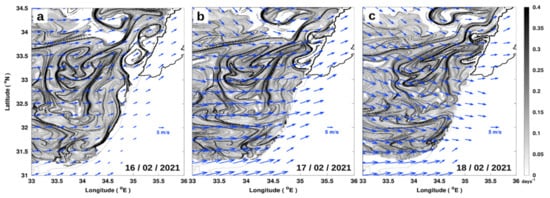
Figure 12.
FSLE maps using surface currents corrected with a wind component for the 16–18th of February 2021 in panels (a–c), respectively. Wind speed is represented as blue vectors in all the panels.
3.4. Prediction of the Lagrangian Front Drifting Speed
3.4.1. Front Drifting Speed in the Area of the East China Sea Oil Spill
We then proceeded with the application of the estimation of the front drifting speed (see Section 2.7) applied to the area of the East China Sea oil spill. Formally, the estimation of the drifting speed of Lagrangian fronts can be derived for fields of both finite-time and finite-size Lyapunov exponents. A visual comparison of the two methods showed that differences were small, and the results qualitatively agree. Since the finite-size technique provided a slightly sharper result (see finite-time Lyapunov exponent result in Figure A4), we reported the analysis based on this diagnostic.
Starting with the velocity fields and FSLE on the 17th of January, we predicted the frontal displacement and the new frontal position over the following two days. Figure 13a represents the Lyapunov exponent fronts for the 17th of January 2018, in the studied area, with the calculated cross-frontal velocities illustrated as purple arrows. The front advection method for the two-day prediction was only applied to the most intense fronts in the area (>0.18 days−1). The results are illustrated as red filaments in Figure 13a, showing the predicted new position of the 17th of January fronts after two days, i.e., on the 19th of January 2018. We then plotted the Lagrangian fronts underlined by the finite-size Lyapunov exponent of the 19th of January, calculated using these interim velocity fields (Figure 13b). The observed “analysis” gray-scaled fronts were then compared to those predicted from the 17th of January FSLE fields (in red). Figure 13b showed a remarkable consistency between the placement of the 19th of January’s analysis ridges (gray-scale) and those, in red, predicted from the 17th of January. The placement of almost all the advected strong fronts for the 19th of January in the studied area was well predicted by this drifting front technique. The persistence from the 17th to the 19th of January of the strong front responsible for stretching the East China Sea oil spill on the 20th of January was an important piece of information. Indeed, we could thus anticipate that sooner or later, the spilled oil would be caught by this nearest strong front and remain in this area.
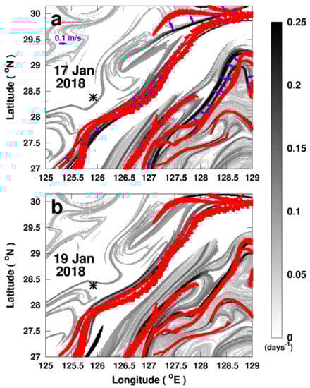
Figure 13.
Comparison of the placement of the predicted fronts by the prediction method to the positions of the real ones derived from the FSLE computation. The red filaments correspond to the new position of the fronts of the 17th of January 2018 (λ > 0.18 days−1) after a 2-day prediction application. The gray-scaled fronts in the background of panels (a,b) are the Lagrangian fronts derived from the FSLE for the 17th and 19th of January 2018, respectively. Panel (a) highlights the drifting for the 17th of January after a 2-day prediction. The purple arrows in (a) are the front drifting speed. Panel (b) allows a comparison between the experimentally-predicted fronts since the 17th of January 2018 (red filaments) and those computed by the FSLE once the required daily velocity fields were available (gray-scaled filaments). The black asterisk indicates the location where the Sanchi tanker sank, engendering the oil discharge.
3.4.2. Front Drifting Speed in the Area of the East Mediterranean Oil Spill
Despite the difficulties in applying the technique in near-shore analyses, we predicted the drifting of the Lagrangian fronts in this region based on the MFS velocity fields and their derived FSLE fields. We started by calculating the speeds at which these fronts, including the one retaining the oil, will move. The resulting drifting velocities were indicated as purple vectors in Figure 14b and applied over the two-day prediction. Figure 14a,b highlighted the initial gray-scaled fronts from the Lyapunov exponent using the initial velocities on the 12th of February 2021. The red filaments in Figure 14b,c revealed the predicted positions of the initial fronts two days later, without using any future data. These were then compared to the FSLE analysis fields on the 14th of February. The predicted eastward drifting towards the shore of the FSLE front that interests us (retaining the oil on the 12th of February) was confirmed by the consistency between the red and gray-scaled fronts in Figure 14c.
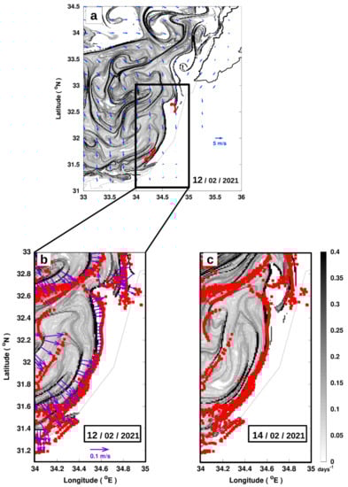
Figure 14.
Two-day prediction from the 12th of February using the developed method with the mixed current. The area of pollution is framed in black in panel (a). The calculated speeds of front drifting are illustrated in panel (b) as purple vectors. The red patterns in panels (b,c) represent the resulting fronts after a 2-day prediction since 12 February. The gray-scaled fronts in the background of panel (b) refer to those of the 12th of February, while the ones in panel (c) are those of the 14th of February. The latter serve for evaluating the placement of the method-derived red fronts.
3.5. Fronts Drift and SST Patterns
In the East China Sea oil spill area, the developed prediction method could reliably predict the displacement and the new positions of Lagrangian fronts governing oil spill dispersion. As previous studies showed an association between Lagrangian and thermal fronts, we investigated whether predicting the near future Lagrangian fronts could also predict future positions of thermal fronts. Conditions of both strong SST contrast and drifting fronts were rare and could not be found at the same time and position of the East China Sea oil spill. However, these two conditions occurred in a nearby region on the 12th of May 2018 (see Figure 15e).

Figure 15.
Lagrangian and thermal fronts drifting. Panel (a) shows the FSLE map of the 12th of May 2018, where a virtual tracer (blue patch) is positioned in the proximity of a Lagrangian front. In panel (b), the gray-scaled Lagrangian fronts are those underlined by the FSLE of the 14th of May 2018. The blue pattern in panel (b) represents the new position of the virtual tracer (released in panel (a)) after a 2-day advection from the 12th of May 2018. Panel (c) is the same FSLE map of the 12th of May 2018 presented in panel (a), where purple arrows reveal the calculated drifting speeds of the fronts with λ > 0.15 days−1. Panel (d) represents the FSLE map of the 14th of May 2018. The 2-day predicted fronts from the 12th of May are superimposed in dark green on both (c,d) maps. These predicted fronts are also added to (e,f) SST maps. (e,f) are the SST maps for the 12th and 14th of May 2018, respectively.
Figure 15a,b endorsed the importance of studying drifting fronts. To investigate whether the front drifting could be predicted, we applied our method to the initial fronts, those of the 12th of May 2018. In Figure 15c, we calculated and drew the drifting speeds as purple vectors. The red fronts in Figure 15c,d were those predicted for the 14th of May, starting from the 12th of May velocities. In Figure 15c, the gray-scaled fronts in the background were derived from the FSLE analysis fields for the 12th of May, whereas those in Figure 15d were from the FSLE analysis fields for the 14th of May. Figure 15d showed a clear consistency between our predicted fronts in red and the analysis fields highlighted by the FSLE in the background.
We proceeded with the SST comparisons. We started by mapping the SST of the 12th of May 2018 in Figure 15e. Then, we superposed the predicted fronts previously calculated for the 14th of January onto the SST of the 14th of May in the background of Figure 15f. By comparing Figure 15f,e, even if it was not conclusive, we could observe certain coherence between the SST spatial pattern and the predicted front on the 14th of May. The SST front seemed to follow the direction of the Lagrangian front drifting, especially the front part retaining the numerical tracer in Figure 15a,b.
4. Discussion
In this paper, we highlighted the ability of near-real-time Lyapunov to predict the stretching dynamics in two cases of medium size (tens of km) oil spills, typical of ship leakages. Moreover, we have highlighted that the Lyapunov vector, an often neglected quantity in the Lyapunov calculation, is able to predict the drifting speed that is also the velocity field orthogonal to the front—and therefore the near-future displacement—of Lagrangian fronts. The implementation of this idea is quite straightforward, the only technical difficulty being the calculation of the tangent to the Lagrangian front, needed to find the component of the velocity field that is orthogonal to the front. This step is easily achieved since the method for the calculation of finite-time/finite-size Lyapunov exponents also provides the Lyapunov vector, which yields the local direction of the Lagrangian front.
Due to the errors in operational velocity fields (either altimetry or assimilation-based models), the simple advection of a numerical tracer released at the position of the accident largely misrepresented the fate of the oil spill. In contrast, we found that a Lyapunov analysis is more informative than simple Lagrangian advection for the two cases of oil spills. In the Sanchi oil spill case, the altimetry-derived geostrophic velocity fields were adequate to identify, in near-real-time, the offshore Lagrangian barriers attracting the propagation of the leaked oil from the 17th to 20th of January 2018. However, conventional altimetry alone was insufficient for detecting near-shore Lagrangian fronts governing the coastal pollution in the Levantine Basin in February 2021. This is not surprising as satellite altimetry products are known to be less reliable over the smaller, more rapidly evolving coastal dynamics. The future SWOT mission, with improved accuracy in coastal regions [60], will allow us to improve the near-coastal analyses. Meanwhile, the near-real-time analyses from the Mediterranean Forecast System model have been shown to detect the Lagrangian front trapping the oil on the 12th and 13th of February 2021. These coastal Lagrangian fronts showed a remarkable susceptibility to wind forcing. The wind strengthening towards the east (after the 16th of February) could move all the fronts in the region at once, following the wind direction. The effect of strong wind had probably helped the pollution reach the eastern Levantine coasts more quickly than from coastal current stirring alone. Moreover, we introduced an avenue to be explored, which is the prediction of future patterns of SST by the developed prediction technique. Even if our results were preliminary and not conclusive, we tracked certain consistency between the predicted Lagrangian fronts and SST patterns. This application should be revisited and repeated using different products, not only SST products with higher resolution but also testing other ecological tracers, such as chlorophyll. The ability to predict these patterns’ deformation may be a promising way to improve conservation studies.
The method we presented based on Lyapunov vectors for predicting front deformation and displacement is a heuristic method based on some assumptions. As a consequence, there are some cases where the front prediction fails. These inconsistencies of the predictive method can be explained by considering the different approximations behind our method. First, possible errors in the convergence of the Lyapunov exponent computation may appear and affect the Lyapunov vector calculation, in particular its orientation. Second, the current velocities may also rapidly change, whereas we are using a constant daily drifting speed for the Lagrangian fronts, which is also the reason why this method remains applicable for short-term predictions only. In this work, we examined two-day predictions as they represent the best compromise to obtain an informative forecast and avoid the errors induced by the rapid change of the current velocities. Predictions of a longer integration time still need further validation work. Third, a limitation of our method is the visual selection of the sharpest fronts in the studied regions. Finally, and most importantly, further developments of a Lyapunov vector-based method for the prediction of a front drifting speed should explicitly estimate all terms that contribute to a material flux across a Lagrangian front, as presented in Shadden et al. (2005) [49] and Haller et al. (2011) [55].
Different biological, physical, and chemical processes (known as oil weathering processes; OWP) may affect the oil patch. OWPs include biodegradation, dissolution, evaporation, and emulsification/dispersion, as well as photo-oxidation [61,62], and depends on the type and characteristics of the oil, as well as on the spatial and temporal environmental conditions. In this work, the two chosen oil spill cases were exclusively used as a validation method for qualifying the efficiency of Lagrangian fronts in affecting the horizontal transport and trajectory of the passive contaminants at the surface. Taking into consideration the weathering processes and different oil types, non-conservative behavior was not crucial in this application but would be important for estimating composition, lifetime, and possible contaminating effect of the oil patch. Nevertheless, in further work, our analyses could benefit from different model-derived data that consider more factors affecting passive pollutants dispersion (e.g., tides and wave forcing).
We assumed that the vertical movement is negligible and focused particularly on the horizontal surface transport. In the eastern Mediterranean, although the pollutant type was reported to be tar oil, we were only interested in analyzing the two slicks floating at the surface. Regarding the East China Sea oil spill, the accident was characterized by the large quantities of condensate, fast-floating ultra-light crude oil (~98% of the total spill) which were released in the ocean, despite the smaller leak of heavy fuel oil (~1.7% of the total spill). Such an accident differs from the ones of previous studies, such as those of the Gulf of Mexico, the Ixtoc (following the explosion of rig off the coast of Mexico in June 1979), and the Deepwater Horizon oil spill studied in the paper of Duran et al. (2018) [27] and which mainly unleashed heavier crude oil that could persist in the deep ocean for years [63,64]. Moreover, natural-gas condensate, as in the East China Sea oil spill, is a petroleum product that is lighter and more volatile than crude oil and that does not last long in the environment. Instead, it burns, evaporates, or degrades, engendering chemical substances in the surface water that last for weeks to months [64]. The short-term predictions studied here are especially relevant for these latter cases.
Our approach is only applicable when stirring by ocean activity is the key mechanism dominating the genesis of the transport patterns, at mesoscales with spatial scales ranging from ~10 to 100 km and on the temporal scales of days to weeks [13,14,15,16].
Usually, when studying horizontal transport, we should take into account the stirring and mixing processes that are the main competitors governing the horizontal transport of tracers in the ocean. Mixing across frontal structures, including diffusivity even in its small-scale, might have an important impact on the dispersion of passive tracers in the ocean. Unlike horizontal stirring that reinforces the tracer gradients across fronts, small-scale diffusivity processes tend to reduce and smooth the gradients [14,65,66]. Nevertheless, in this study, we particularly highlighted the impact of the horizontal stirring in controlling the formation and the evolution of the transport patterns, shaping, in turn, the trajectory of the oil tracer. When neglecting the impact of cross-front diffusivity, we assume a scale separation and emphasize the balance between the mesoscale straining of a frontal structure and the small-scale mixing across the front (the Lagrangian front in our case). Under this assumption, the mesoscale stirring leads, at first, to a stretching of the patch by the currents along one direction while reducing the other, thus forming an elongated filament-shaped front. The profile of the tracer patch with its initial centered origin is transformed into a half Gaussian curve [41]. The continuous effect of this filamentation process creates more surfaces of contact along the stretching direction between regions of distinct properties. Simultaneously, the width of the front keeps thinning until the impact of smaller-scale across-front diffusion arises and balances that of the mesoscale straining [41,67,68].
The following scale equation defines the balance between mixing and stirring processes.
where KH represents the small-scale diffusivity and λ determines the larger scale strain rate. The latter refers, in our case, to the stretching rate of the front and thus to the associated Lyapunov exponent quantity [41,67,68]. According to Nencioli et al. (2013) [68], the cross-front mean diffusivity KH is estimated at 3.98 m2 s−1 with 70% of the obtained KH values ranging between 0.4 and 5 m2 s−1. The equation of σ as a function of KH and λ represents the scale at which the stirring and diffusivity impacts are balanced. For spatial scales larger than σ, the strain impact dominates the small-scale mixing in the horizontal processes. However, at scales smaller than σ, reliable work should take into account the significant diffusivity contribution associated with the fronts. In our study on the East China Sea oil spill, we found λ = ~0.18 days−1 as the minimal strain value for the sharpest Lyapunov fronts. For such a strain rate, the scale parameter, σ, can be calculated following Equation (2). The mean σ in the area of the East China Sea oil spill is thus estimated to be ~1.38 km (~0.44–1.55 km). For the East Mediterranean oil spill case, with a mean Lyapunov exponent of 0.31 days−1, the mean σ is 1.05 km (~0.33–1.18 km).
Our studied processes extend on a scale area (>10 km) larger than the scale parameter with a particular focus on the mesoscale dynamics. The assumption of neglecting the small-scale diffusivity impact across the front in this work is thus consistent with these scales.
5. Conclusions
In this work, we studied the capacity of Lagrangian methods in informing on the shape and drift of oil spills of medium size (~10 s of km), such as the ones that may be caused by a ship leakage. Lagrangian advection of virtual tracers cannot sufficiently represent the path of oil spills, mainly due to the fact that available model- or altimetry-based velocity fields are too smooth. As a consequence, the virtual patch is insufficiently stretched and insufficiently drifts in respect to the real one. However, the computation of Lagrangian fronts through the Lyapunov exponent calculation allows the detection of near-real-time stirring features, the Lagrangian fronts, predicting where the tracer is being attracted and filamented. Our analysis shows that these Lagrangian structures are vulnerable to strong wind events that can, at once (in a few hours), break them or move them abruptly to the coast. Aside from near-real-time studies, pollution management demands knowledge of the future propagation of the pollutant in the days following the discharge. We showed that under some approximations, this information can be estimated by combining the near-real-time Lyapunov vector and near-real-time surface currents, without the need for information on future current velocities. This prediction can work on short-term studies (2–3 days) and can support management and prediction tools for oil spills and other floating contaminants. Our approach will undoubtedly benefit from future satellite altimetry missions, such as SWOT [56,69,70], in terms of their observations with increased resolution and reliability close to the coast, and may be extended to other environmental applications, such as conservation [52].
Author Contributions
Conceptualization, G.F. and F.d.; methodology, G.F. and F.d.; software, G.F., F.d., G.B. and A.B.; validation, G.F. and F.d.; formal analysis, G.F. and F.d.; investigation, G.F., Y.F. and F.d.; resources, Y.F.; data curation, G.F., F.d. and Y.F.; writing—original draft preparation, G.F.; writing—review and editing, F.d., R.M., A.B., M.F., G.B., Y.F., L.M. and G.F.; visualization, G.F. and F.d.; supervision, F.d. and M.F.; project administration, F.d. and M.F.; funding acquisition, M.F. and F.d. All authors have read and agreed to the published version of the manuscript.
Funding
The authors would like to acknowledge the National Council for Scientific Research of Lebanon (CNRS-L) for granting a doctoral fellowship to G.F. This work has been supported by CNES through the Tosca BIOSWOT-AdAC project and partially funded by the ALTILEV program in the framework of the PHC-CEDRE project.
Data Availability Statement
The authors confirm that the data supporting the findings of this study are cited within the article.
Acknowledgments
The authors would like to thank all the people who contributed to this work. We gratefully acknowledge the French Institute Collecte Localisation Satellites (CLS) in Brest for providing us with the data for the oil spill trajectories, and in particular, Patrick Leildé, for performing the SAR Satellite Imagery Analysis.
Conflicts of Interest
The authors declare no conflict of interest.
Appendix A
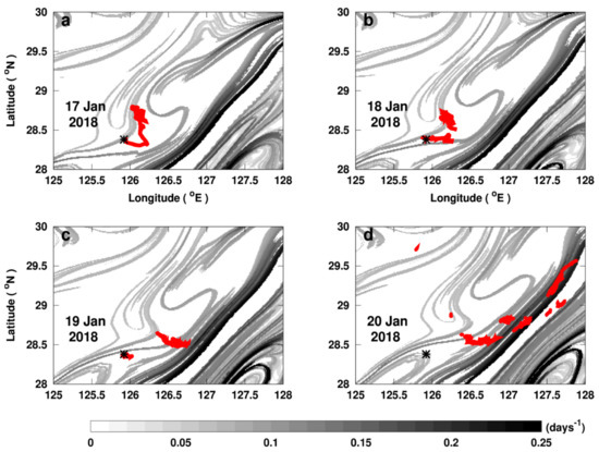
Figure A1.
Daily backward finite-size Lyapunov exponent (FSLE) application repeated in the area of the East China Sea oil spill using the altimetry product in delayed-time. The black asterisk in all panels indicates the location where the Sanchi tanker sank. The red patch represents the daily evolution of the Sanchi leaked oil path from the 17th to 20th of January 2018 in panels (a–d), respectively. The gray-scaled filament-shaped fronts in the background represent daily Lagrangian fronts (FSLE computation using Altimetry Copernicus product in delayed-time). The altimetry-derived velocity product in delayed-time used here is available at E.U. Copernicus Marine Service Information (CMEMS). Daily surface observations of the global ocean are used in delayed-time (DT), with L4 processing level and a spatial resolution accounting for 0.25° × 0.25° (product id: SEALEVEL_GLO_PHY_L4_REP_OBSERVATIONS_008_047).
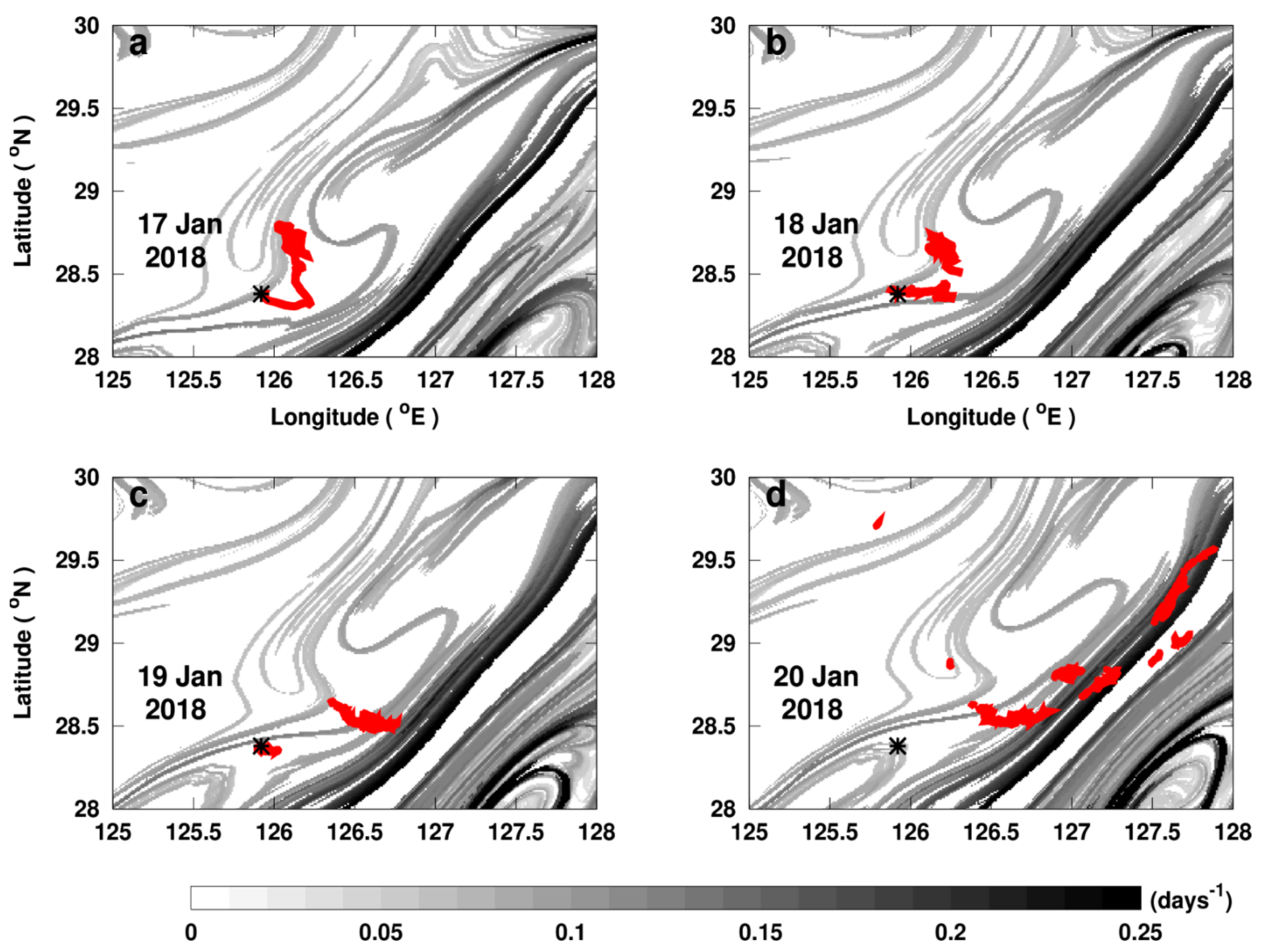
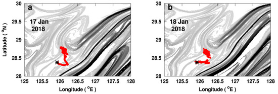
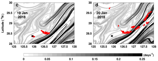
Figure A2.
Daily backward finite-size Lyapunov exponent (FSLE) application in the area of the East China Sea oil spill using altimetry and the Ekman product. The black asterisk in all panels indicates the location where the Sanchi tanker sank. The red patch represents the daily evolution of the Sanchi leaked oil path from the 17th to 20th of January 2018 in panels (a–d), respectively. The gray-scaled filament-shaped fronts in the background represent daily Lagrangian fronts (FSLE computation using altimetry and the Ekman Copernicus product). The Ekman product, where geostrophic velocity fields are combined with modeled Ekman current, is available at E.U. Copernicus Marine Service Information (CMEMS). Daily global ocean products are used with 0.25° × 0.25° spatial resolution and L4 processing level (product id: MULTIOBS_GLO_PHY_NRT_015_003).

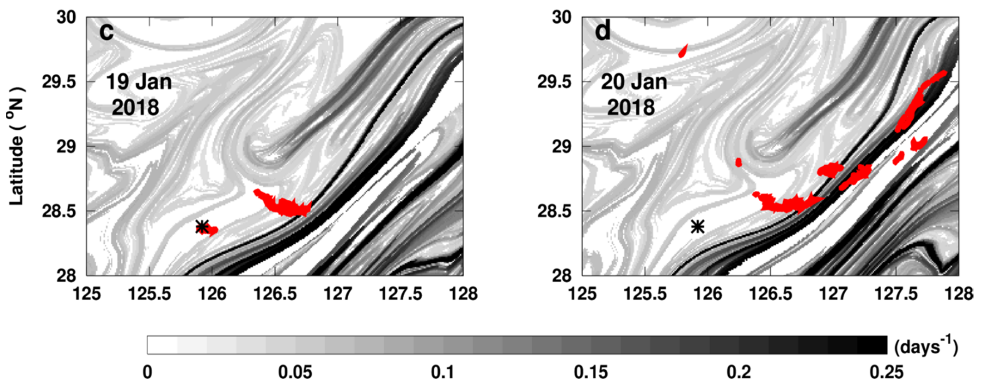
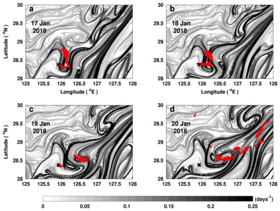
Figure A3.
Daily backward finite-size Lyapunov exponent (FSLE) application in the area of the East China Sea oil spill using Mercator analysis product. The black asterisk in all panels indicates the location where the Sanchi tanker sank. The red patch represents the daily evolution of the Sanchi leaked oil path from the 17th to 20th of January 2018 in panels (a–d), respectively. The gray-scaled filament-shaped fronts in the background represent daily Lagrangian fronts (FSLE computation using Mercator analysis Copernicus product (product id: GLOBAL_ANALYSIS_FORECAST_PHY_001_024)). Surface daily-mean current velocities are considered, with 0.083° × 0.083° spatial resolution and L4 processing level.

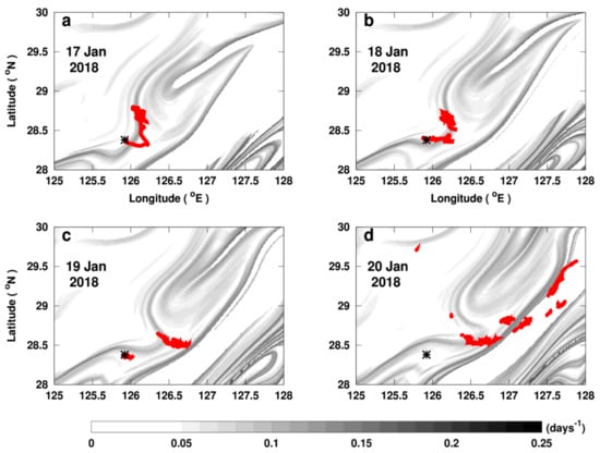
Figure A4.
Daily backward finite-time Lyapunov exponent (FTLE) application in the area of the East China Sea oil spill using the altimetry product in near-real-time. The black asterisk in all panels indicates the location where the Sanchi tanker sank. The red patch represents the daily evolution of Sanchi leaked oil path from the 17th to 20th of January 2018 in panels (a–d), respectively. The gray-scaled filament-shaped fronts in the background represent daily Lagrangian fronts (FTLE computation using Altimetry Copernicus product). Dark fronts reveal highly attractive and stretching zones. In this case, the sharpest front is related to the core of the Kuroshio Current. These fronts are even more prominently observed with the backward FSLE technique. The altimetry-derived velocity product is also available at E.U. Copernicus Marine Service Information (CMEMS). Daily surface observations of the global ocean are used in near-real-time (NRT), with L4 processing level and a spatial resolution accounting for 0.25° × 0.25° (product id: SEALEVEL_GLO_PHY_L4_NRT_OBSERVATIONS_008_046).
References
- Rathore, S.S.; Chandravanshi, P.; Chandravanshi, A.; Jaiswal, K. Eutrophication: Impacts of Excess Nutrient Inputs on Aquatic Ecosystem. IOSR 2016, 9, 89–96. [Google Scholar] [CrossRef]
- Wurtsbaugh, W.A.; Paerl, H.W.; Dodds, W.K. Nutrients, Eutrophication and Harmful Algal Blooms along the Freshwater to Marine Continuum. WIREs Water 2019, 6, e1373. [Google Scholar] [CrossRef]
- Ma, Y.; Halsall, C.J.; Crosse, J.D.; Graf, C.; Cai, M.; He, J.; Gao, G.; Jones, K. Persistent Organic Pollutants in Ocean Sediments from the N orth P acific to the Arctic O cean. J. Geophys. Res. Oceans 2015, 120, 2723–2735. [Google Scholar] [CrossRef] [Green Version]
- Michel, J.; Fingas, M. Oil Spills: Causes, Consequences, Prevention, and Countermeasures. In World Scientific Series in Current Energy Issues; World Scientific: Singapore, 2016; Volume 1, pp. 159–201. ISBN 978-981-4699-97-6. [Google Scholar]
- Furness, R.W.; Rainbow, P.S. Heavy Metals in the Marine Environment; CRC Press: Boca Raton, FL, USA, 2018; ISBN 978-1-351-07315-8. [Google Scholar]
- Szefer, P. Metal Pollutants and Radionuclides in the Baltic Sea—An Overview. Oceanologia 2002, 44, 129–178. [Google Scholar]
- Prants, S.V.; Budyansky, M.V.; Uleysky, M.Y. Lagrangian Study of Surface Transport in the Kuroshio Extension Area Based on Simulation of Propagation of Fukushima-Derived Radionuclides. Nonlinear Processes Geophys. 2014, 21, 279–289. [Google Scholar] [CrossRef] [Green Version]
- Ramirez-Llodra, E.; De Mol, B.; Company, J.B.; Coll, M.; Sardà, F. Effects of Natural and Anthropogenic Processes in the Distribution of Marine Litter in the Deep Mediterranean Sea. Progress Oceanogr. 2013, 118, 273–287. [Google Scholar] [CrossRef]
- Islam, S.; Tanaka, M. Impacts of Pollution on Coastal and Marine Ecosystems Including Coastal and Marine Fisheries and Approach for Management: A Review and Synthesis. Mar. Pollut. Bull. 2004, 48, 624–649. [Google Scholar] [CrossRef] [PubMed]
- Worm, B.; Lotze, H.K.; Jubinville, I.; Wilcox, C.; Jambeck, J. Plastic as a Persistent Marine Pollutant. Annu. Rev. Environ. Resour. 2017, 42, 1–26. [Google Scholar] [CrossRef]
- Sumaila, U.R.; Cisneros-Montemayor, A.M.; Dyck, A.; Huang, L.; Cheung, W.; Jacquet, J.; Kleisner, K.; Lam, V.; McCrea-Strub, A.; Swartz, W.; et al. Impact of the Deepwater Horizon Well Blowout on the Economics of US Gulf Fisheries. Can. J. Fish. Aquat. Sci. 2012, 69, 499–510. [Google Scholar] [CrossRef] [Green Version]
- Beaumont, N.J.; Aanesen, M.; Austen, M.C.; Börger, T.; Clark, J.R.; Cole, M.; Hooper, T.; Lindeque, P.K.; Pascoe, C.; Wyles, K.J. Global Ecological, Social and Economic Impacts of Marine Plastic. Mar. Pollut. Bull. 2019, 142, 189–195. [Google Scholar] [CrossRef]
- Danabasoglu, G.; McWilliams, J.C.; Gent, P.R. The Role of Mesoscale Tracer Transports in the Global Ocean Circulation. Science 1994, 264, 1123–1126. [Google Scholar] [CrossRef] [PubMed]
- D’ovidio, F.; Della Penna, A.; Trull, T.W.; Nencioli, F.; Pujol, M.-I.; Rio, M.-H.; Park, Y.-H.; Cotté, C.; Zhou, M.; Blain, S. The Biogeochemical Structuring Role of Horizontal Stirring: Lagrangian Perspectives on Iron Delivery Downstream of the Kerguelen Plateau. Biogeosciences 2015, 12, 5567–5581. [Google Scholar] [CrossRef] [Green Version]
- García-Olivares, A.; Isern-Fontanet, J.; García-Ladona, E. Dispersion of Passive Tracers and Finite-Scale Lyapunov Exponents in the Western Mediterranean Sea. Deep Sea Res. Part I Oceanogr. Res. Pap. 2007, 54, 253–268. [Google Scholar] [CrossRef]
- Baudena, A.; Ser-Giacomi, E.; López, C.; Hernández-García, E.; d’Ovidio, F. Crossroads of the Mesoscale Circulation. J. Mar. Syst. 2019, 192, 1–14. [Google Scholar] [CrossRef] [Green Version]
- Musa, Z.N.; Popescu, I.; Mynett, A. A Review of Applications of Satellite SAR, Optical, Altimetry and DEM Data for Surface Water Modelling, Mapping and Parameter Estimation. Hydrol. Earth Syst. Sci. 2015, 19, 3755–3769. [Google Scholar] [CrossRef] [Green Version]
- Haza, A.C.; Özgökmen, T.M.; Griffa, A.; Garraffo, Z.D.; Piterbarg, L. Parameterization of Particle Transport at Submesoscales in the Gulf Stream Region Using Lagrangian Subgridscale Models. Ocean Model. 2012, 42, 31–49. [Google Scholar] [CrossRef]
- Prants, S.V.; Uleysky, M.Y.; Budyansky, M.V. Lagrangian Coherent Structures in the Ocean Favorable for Fishery. Dokl. Earth Sci. 2012, 447, 1269–1272. [Google Scholar] [CrossRef]
- Gildor, H.; Fredj, E.; Steinbuck, J.; Monismith, S. Evidence for Submesoscale Barriers to Horizontal Mixing in the Ocean from Current Measurements and Aerial Photographs. J. Phys. Oceanogr. 2009, 39, 1975–1983. [Google Scholar] [CrossRef]
- McWilliams, J.C. Submesoscale Currents in the Ocean. Proc. R. Soc. A 2016, 472, 20160117. [Google Scholar] [CrossRef]
- Van Sebille, E.; Griffies, S.M.; Abernathey, R.; Adams, T.P.; Berloff, P.; Biastoch, A.; Blanke, B.; Chassignet, E.P.; Cheng, Y.; Cotter, C.J.; et al. Lagrangian Ocean Analysis: Fundamentals and Practices. Ocean Model. 2018, 121, 49–75. [Google Scholar] [CrossRef]
- Boffetta, G.; Lacorata, G.; Redaelli, G.; Vulpiani, A. Detecting Barriers to Transport: A Review of Different Techniques. Phys. D Nonlinear Phenom. 2001, 159, 58–70. [Google Scholar] [CrossRef] [Green Version]
- Haller, G.; Yuan, G. Lagrangian Coherent Structures and Mixing in Two-Dimensional Turbulence. Phys. D Nonlinear Phenom. 2000, 147, 352–370. [Google Scholar] [CrossRef]
- Lehahn, Y.; d’Ovidio, F.; Koren, I. A Satellite-Based Lagrangian View on Phytoplankton Dynamics. Annu. Rev. Mar. Sci. 2018, 10, 99–119. [Google Scholar] [CrossRef] [Green Version]
- Olascoaga, M.J.; Haller, G. Forecasting Sudden Changes in Environmental Pollution Patterns. Proc. Natl. Acad. Sci. USA 2012, 109, 4738–4743. [Google Scholar] [CrossRef] [PubMed] [Green Version]
- Duran, R.; Beron-Vera, F.J.; Olascoaga, M.J. Extracting Quasi-Steady Lagrangian Transport Patterns from the Ocean Circulation: An Application to the Gulf of Mexico. Sci. Rep. 2018, 8, 5218. [Google Scholar] [CrossRef] [PubMed] [Green Version]
- Sun, S.; Lu, Y.; Liu, Y.; Wang, M.; Hu, C. Tracking an Oil Tanker Collision and Spilled Oils in the East China Sea Using Multisensor Day and Night Satellite Imagery. Geophys. Res. Lett. 2018, 45, 3212–3220. [Google Scholar] [CrossRef]
- Yin, L.; Zhang, M.; Zhang, Y.; Qiao, F. The Long-Term Prediction of the Oil-Contaminated Water from the Sanchi Collision in the East China Sea. Acta Oceanol. Sin. 2018, 37, 69–72. [Google Scholar] [CrossRef]
- Amir-Heidari, P.; Raie, M. Response Planning for Accidental Oil Spills in Persian Gulf: A Decision Support System (DSS) Based on Consequence Modeling. Mar. Pollut. Bull. 2019, 140, 116–128. [Google Scholar] [CrossRef]
- Pan, Q.; Yu, H.; Daling, P.S.; Zhang, Y.; Reed, M.; Wang, Z.; Li, Y.; Wang, X.; Wu, L.; Zhang, Z.; et al. Fate and Behavior of Sanchi Oil Spill Transported by the Kuroshio during January–February 2018. Mar. Pollut. Bull. 2020, 152, 110917. [Google Scholar] [CrossRef] [PubMed]
- Gallagher, S.J.; Kitamura, A.; Iryu, Y.; Itaki, T.; Koizumi, I.; Hoiles, P.W. The Pliocene to Recent History of the Kuroshio and Tsushima Currents: A Multi-Proxy Approach. Prog. Earth Planet. Sci. 2015, 2, 17. [Google Scholar] [CrossRef] [Green Version]
- Abdulla, A.; Linden, O. Maritime Traffic Effects on Biodiversity in the Mediterranean Sea: Review of Impacts, Priority Areas and Mitigation Measures; IUCN: Gland, Switzerland, 2008; ISBN 978-2-8317-1079-2. [Google Scholar]
- Coomber, F.G.; D’Incà, M.; Rosso, M.; Tepsich, P.; di Sciara, G.N.; Moulins, A. Description of the Vessel Traffic within the North Pelagos Sanctuary: Inputs for Marine Spatial Planning and Management Implications within an Existing International Marine Protected Area. Mar. Policy 2016, 69, 102–113. [Google Scholar] [CrossRef]
- Bonanno, A.; Zgozi, S.W.; Jarboui, O.; Mifsud, R.; Ceriola, L.; Basilone, G.; Arneri, E. Marine Ecosystems and Living Resources in the Central Mediterranean Sea: An Introduction. Hydrobiologia 2018, 821, 1–10. [Google Scholar] [CrossRef] [Green Version]
- Marangoni, C. Sul principio della viscosita’ superficiale dei liquidi stabilito dalsig. J. Plateau. Nuovo Cimento 1871, 5–6, 239–273. [Google Scholar] [CrossRef]
- Alpers, W.; Hühnerfuss, H. Radar Signatures of Oil Films Floating on the Sea Surface and the Marangoni Effect. J. Geophys. Res. 1988, 93, 3642. [Google Scholar] [CrossRef]
- Jackson, C.R.; Apel, J.R. Synthetic Aperture Radar: Marine User’s Manual; U.S. Dept. of Commerce, National Oceanic and Atmospheric Administration, National Environmental Satellite, Data, and Information Service, Office of Research and Applications: Washington, DC, USA, 2004; ISBN 978-0-16-073214-0.
- Girard-Ardhuin, F.; Mercier, G.; Collard, F.; Garello, R. Operational Oil-Slick Characterization by SAR Imagery and Synergistic Data. IEEE J. Ocean. Eng. 2005, 30, 487–495. [Google Scholar] [CrossRef] [Green Version]
- Press, W.H.; Teukolsky, S.A.; Flannery, B.P.; Vetterling, W.T. Numerical Recipes in Fortran 77: Volume 1, Volume 1 of Fortran Numerical Recipes: The Art of Scientific Computing; Cambridge University Press: Cambridge, UK, 1992; ISBN 978-0-521-43108-8. [Google Scholar]
- Abraham, E.R.; Law, C.S.; Boyd, P.W.; Lavender, S.J.; Maldonado, M.T.; Bowie, A.R. Importance of Stirring in the Development of an Iron-Fertilized Phytoplankton Bloom. Nature 2000, 407, 727–730. [Google Scholar] [CrossRef]
- D’Ovidio, F.; Fernández, V.; Hernández-García, E.; López, C. Mixing Structures in the Mediterranean Sea from Finite-Size Lyapunov Exponents. Geophys. Res. Lett. 2004, 31, L17203. [Google Scholar] [CrossRef] [Green Version]
- Haller, G. Lagrangian Coherent Structures. Annu. Rev. Fluid Mech. 2015, 47, 137–162. [Google Scholar] [CrossRef] [Green Version]
- Ott, E. Chaos in Dynamical Systems; Cambridge University Press: Cambridge, UK; New York, NY, USA, 2002; ISBN 978-0-521-81196-5. [Google Scholar]
- Koh, T.-Y.; Legras, B. Hyperbolic Lines and the Stratospheric Polar Vortex. Chaos 2002, 12, 382–394. [Google Scholar] [CrossRef]
- Pierrehumbert, R.T.; Yang, H. Global Chaotic Mixing on Isentropic Surfaces. J. Atmos. Sci. 1993, 50, 2462–2480. [Google Scholar] [CrossRef] [Green Version]
- Tél, T.; de Moura, A.; Grebogi, C.; Károlyi, G. Chemical and Biological Activity in Open Flows: A Dynamical System Approach. Phys. Rep. 2005, 413, 91–196. [Google Scholar] [CrossRef]
- D’Ovidio, F.; Shuckburgh, E.; Legras, B. Local Mixing Events in the Upper Troposphere and Lower Stratosphere. Part I: Detection with the Lyapunov Diffusivity. J. Atmos. Sci. 2009, 66, 3678–3694. [Google Scholar] [CrossRef]
- Bettencourt, J.H.; López, C.; Hernández-García, E.; Montes, I.; Sudre, J.; Dewitte, B.; Paulmier, A.; Garçon, V. Boundaries of the Peruvian Oxygen Minimum Zone Shaped by Coherent Mesoscale Dynamics. Nat. Geosci. 2015, 8, 937–940. [Google Scholar] [CrossRef] [Green Version]
- Hernández-Carrasco, I.; López, C.; Hernández-García, E.; Turiel, A. Seasonal and Regional Characterization of Horizontal Stirring in the Global Ocean. J. Geophys. Res. 2012, 117, C10007. [Google Scholar] [CrossRef] [Green Version]
- Rossi, V.; López, C.; Sudre, J.; Hernández-García, E.; Garçon, V. Comparative Study of Mixing and Biological Activity of the Benguela and Canary Upwelling Systems. Geophys. Res. Lett. 2008, 35, L11602. [Google Scholar] [CrossRef] [Green Version]
- Della Penna, A.; Koubbi, P.; Cotté, C.; Bon, C.; Bost, C.-A.; d’Ovidio, F. Lagrangian Analysis of Multi-Satellite Data in Support of Open Ocean Marine Protected Area Design. Deep Sea Res. Part II Top. Stud. Oceanogr. 2017, 140, 212–221. [Google Scholar] [CrossRef]
- Bettencourt, J.H.; Rossi, V.; Hernández-García, E.; Marta-Almeida, M.; López, C. Characterization of the Structure and Cross-shore Transport Properties of a Coastal Upwelling Filament Using Three-dimensional Finite-size Lyapunov Exponents. J. Geophys. Res. Oceans 2017, 122, 7433–7448. [Google Scholar] [CrossRef] [Green Version]
- Shadden, S.C.; Lekien, F.; Marsden, J.E. Definition and Properties of Lagrangian Coherent Structures from Finite-Time Lyapunov Exponents in Two-Dimensional Aperiodic Flows. Phys. D Nonlinear Phenom. 2005, 212, 271–304. [Google Scholar] [CrossRef]
- Haller, G. A Variational Theory of Hyperbolic Lagrangian Coherent Structures. Phys. D Nonlinear Phenom. 2011, 240, 574–598. [Google Scholar] [CrossRef]
- Barceló-Llull, B.; Pascual, A.; Sánchez-Román, A.; Cutolo, E.; d’Ovidio, F.; Fifani, G.; Ser-Giacomi, E.; Ruiz, S.; Mason, E.; Cyr, F.; et al. Fine-Scale Ocean Currents Derived From in Situ Observations in Anticipation of the Upcoming SWOT Altimetric Mission. Front. Mar. Sci. 2021, 8, 679844. [Google Scholar] [CrossRef]
- Baaklini, G.; Issa, L.; Fakhri, M.; Brajard, J.; Fifani, G.; Menna, M.; Taupier-Letage, I.; Bosse, A.; Mortier, L. Blending Drifters and Altimetric Data to Estimate Surface Currents: Application in the Levantine Mediterranean and Objective Validation with Different Data Types. Ocean Model. 2021, 166, 101850. [Google Scholar] [CrossRef]
- Cipollini, P.; Vignudelli, S.; Benveniste, J. The Coastal Zone: A Mission Target for Satellite Altimeters: Summary of the 7th Coastal Altimetry Workshop; Boulder, Colorado, 7–8 October 2013. Eos Trans. AGU 2014, 95, 72. [Google Scholar] [CrossRef] [Green Version]
- Ballarotta, M.; Ubelmann, C.; Pujol, M.-I.; Taburet, G.; Fournier, F.; Legeais, J.-F.; Faugère, Y.; Delepoulle, A.; Chelton, D.; Dibarboure, G.; et al. On the Resolutions of Ocean Altimetry Maps. Ocean Sci. 2019, 15, 1091–1109. [Google Scholar] [CrossRef] [Green Version]
- Vignudelli, S.; Birol, F.; Benveniste, J.; Fu, L.-L.; Picot, N.; Raynal, M.; Roinard, H. Satellite Altimetry Measurements of Sea Level in the Coastal Zone. Surv. Geophys. 2019, 40, 1319–1349. [Google Scholar] [CrossRef]
- Forth, H.P.; Mitchelmore, C.L.; Morris, J.M.; Lipton, J. Characterization of Oil and Water Accommodated Fractions Used to Conduct Aquatic Toxicity Testing in Support of the Deepwater Horizon Oil Spill Natural Resource Damage Assessment: Characterization of Oil and Water Accommodated Fractions. Environ. Toxicol. Chem. 2017, 36, 1450–1459. [Google Scholar] [CrossRef] [PubMed]
- Drouin, K.L.; Mariano, A.J.; Ryan, E.H.; Laurindo, L.C. Lagrangian Simulation of Oil Trajectories in the Florida Straits. Mar. Pollut. Bull. 2019, 140, 204–218. [Google Scholar] [CrossRef]
- Soto, L.A.; Botello, A.V.; Licea-Durán, S.; Lizárraga-Partida, M.L.; Yáñez-Arancibia, A. The Environmental Legacy of the Ixtoc-I Oil Spill in Campeche Sound, Southwestern Gulf of Mexico. Front. Mar. Sci. 2014, 1, 1–9. [Google Scholar] [CrossRef] [Green Version]
- Carswell, C. Unique Oil Spill in East China Sea Frustrates Scientists. Nature 2018, 554, 17–19. [Google Scholar] [CrossRef] [Green Version]
- Sundermeyer, M.A.; Price, J.F. Lateral Mixing and the North Atlantic Tracer Release Experiment: Observations and Numerical Simulations of Lagrangian Particles and a Passive Tracer. J. Geophys. Res. 1998, 103, 21481–21497. [Google Scholar] [CrossRef] [Green Version]
- Baudena, A.; Ser-Giacomi, E.; D’Onofrio, D.; Capet, X.; Cotté, C.; Cherel, Y.; D’Ovidio, F. Fine-Scale Structures as Spots of Increased Fish Concentration in the Open Ocean. Sci. Rep. 2021, 11, 15805. [Google Scholar] [CrossRef]
- Ledwell, J.R.; Watson, A.J.; Law, C.S. Mixing of a Tracer in the Pycnocline. J. Geophys. Res. 1998, 103, 21499–21529. [Google Scholar] [CrossRef]
- Nencioli, F.; d’Ovidio, F.; Doglioli, A.M.; Petrenko, A.A. In Situ Estimates of Submesoscale Horizontal Eddy Diffusivity across an Ocean Front. J. Geophys. Res. Oceans 2013, 118, 7066–7080. [Google Scholar] [CrossRef] [Green Version]
- Morrow, R.; Fu, L.-L.; Ardhuin, F.; Benkiran, M.; Chapron, B.; Cosme, E.; d’Ovidio, F.; Farrar, J.T.; Gille, S.T.; Lapeyre, G.; et al. Global Observations of Fine-Scale Ocean Surface Topography With the Surface Water and Ocean Topography (SWOT) Mission. Front. Mar. Sci. 2019, 6, 232. [Google Scholar] [CrossRef]
- d’Ovidio, F.; Pascual, A.; Wang, J.; Doglioli, A.M.; Jing, Z.; Moreau, S.; Grégori, G.; Swart, S.; Speich, S.; Cyr, F.; et al. Frontiers in Fine-Scale in Situ Studies: Opportunities During the SWOT Fast Sampling Phase. Front. Mar. Sci. 2019, 6, 168. [Google Scholar] [CrossRef]
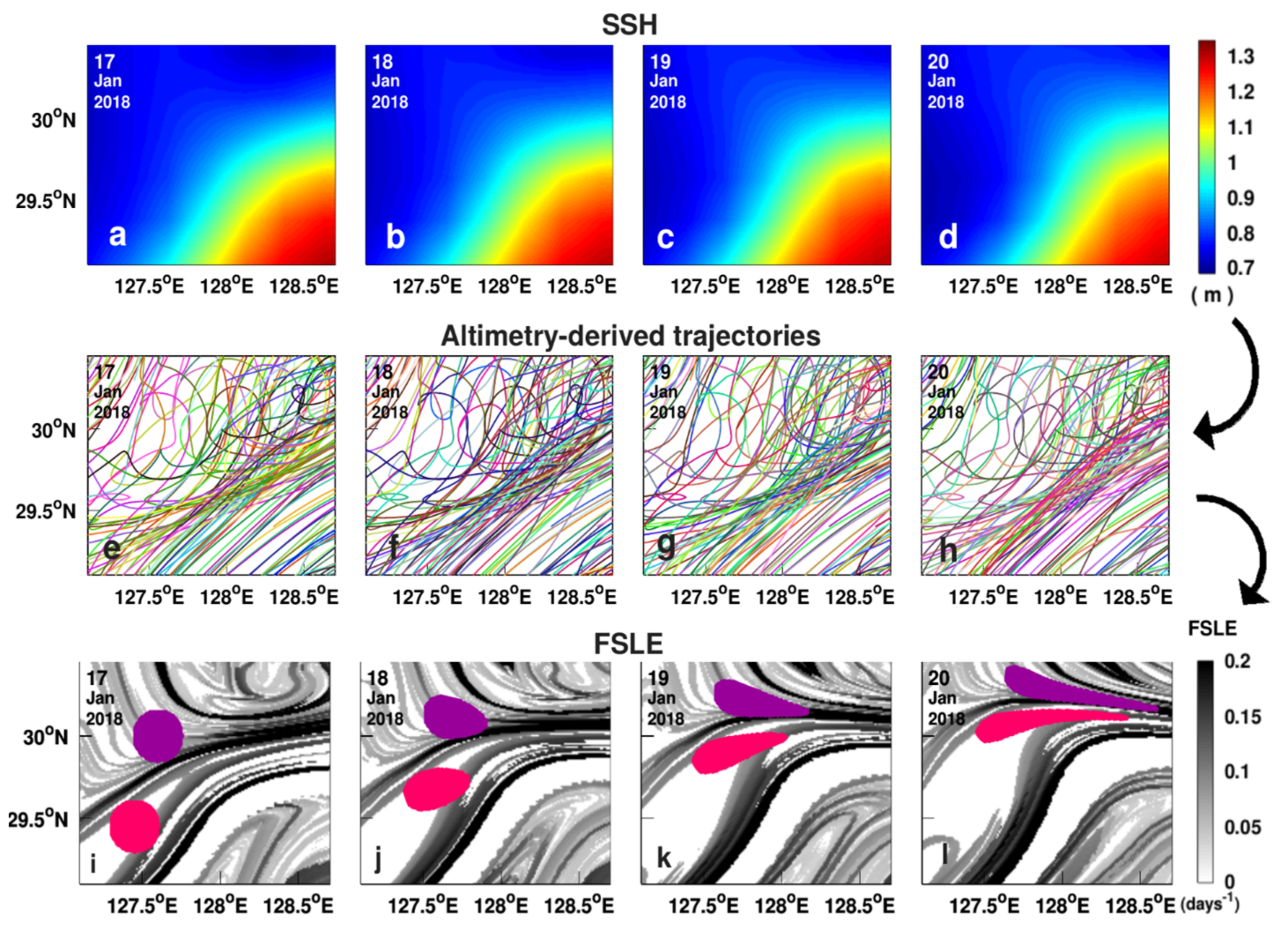
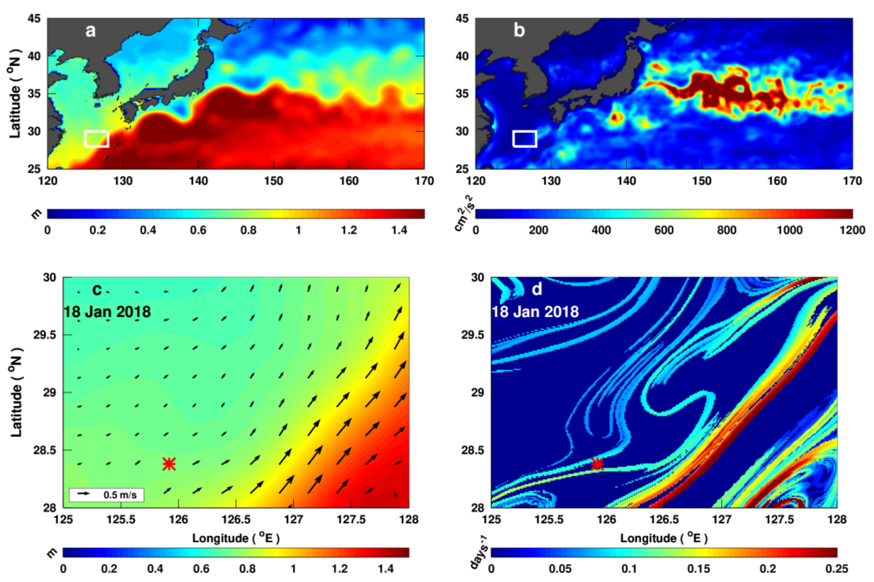
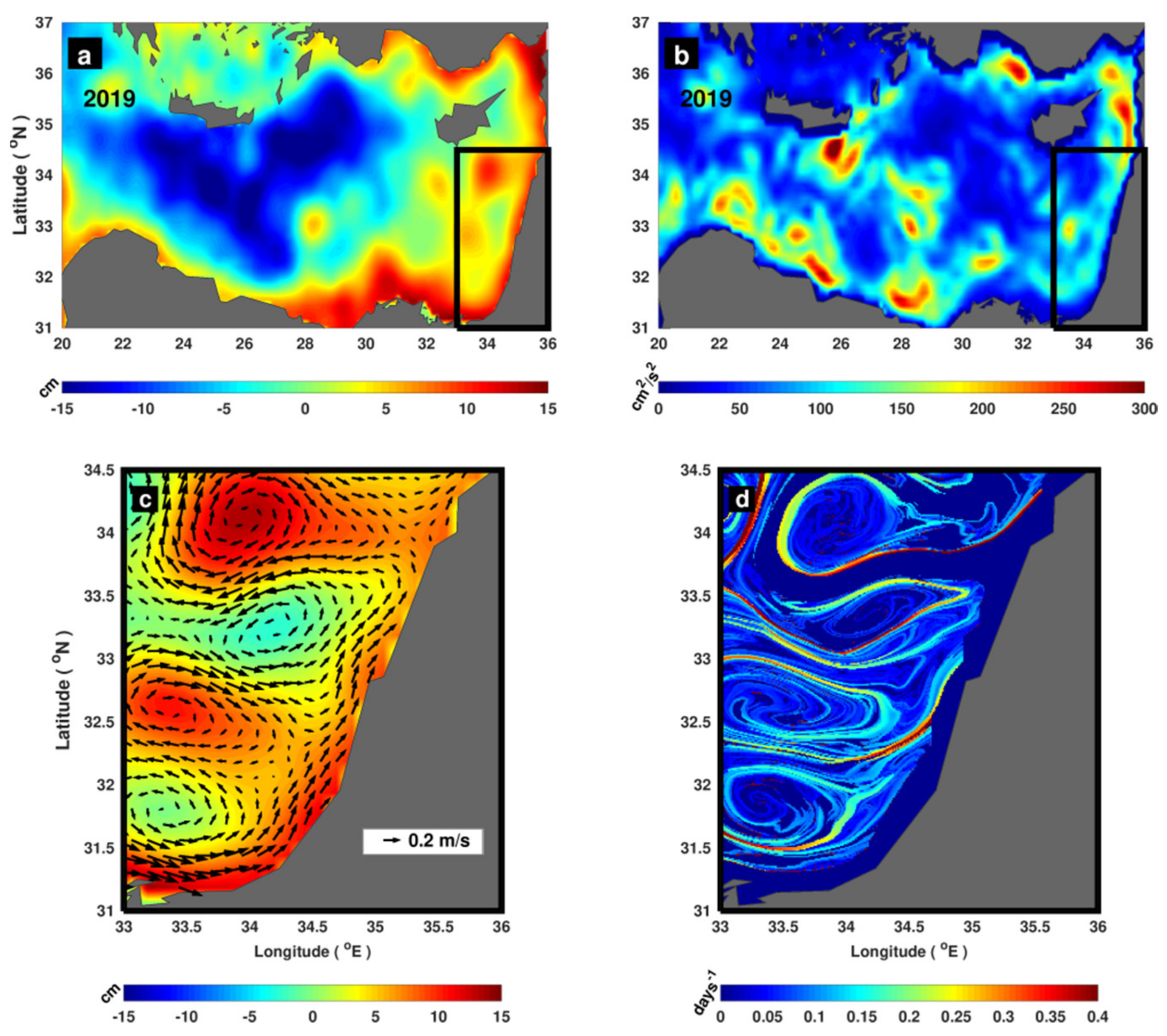
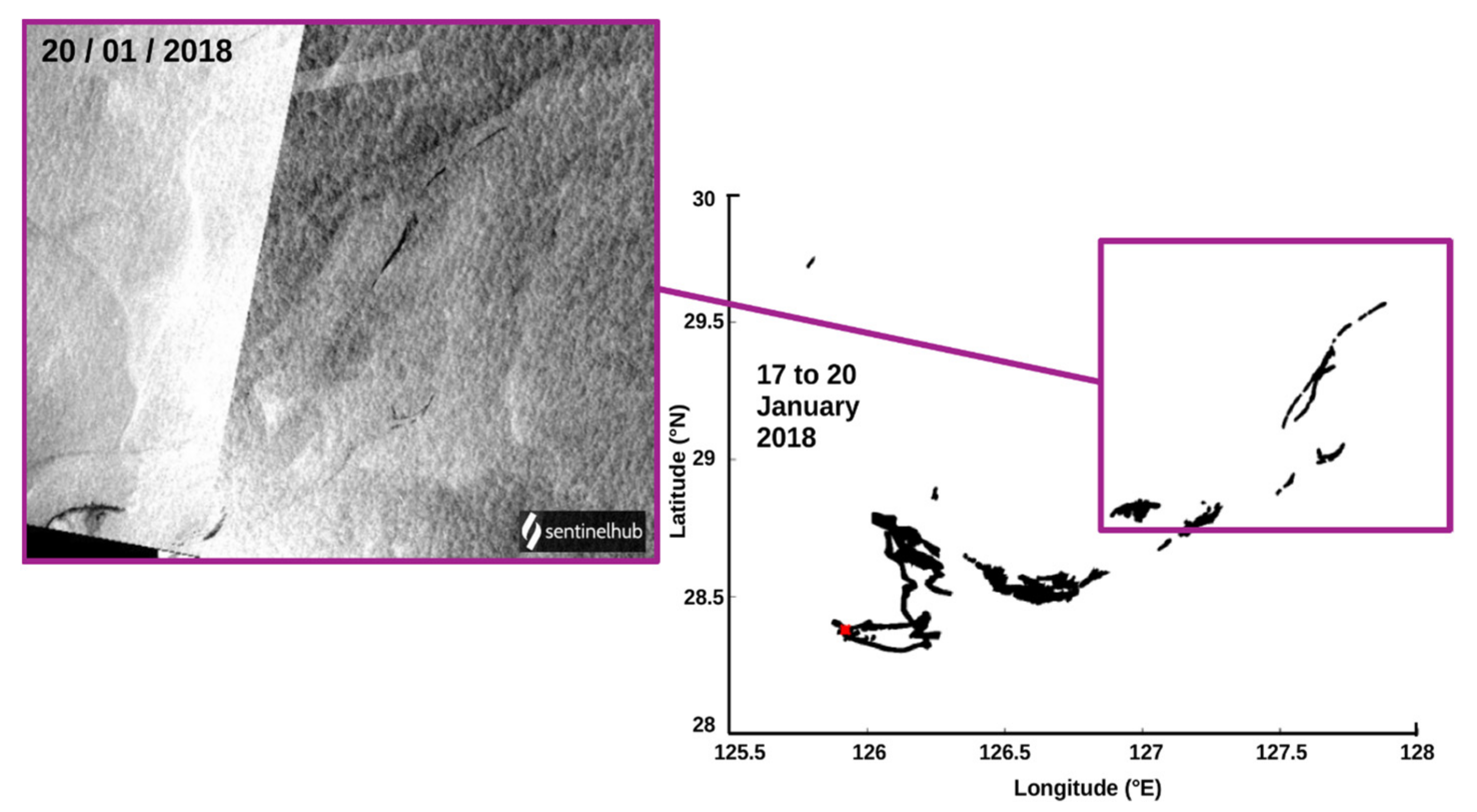

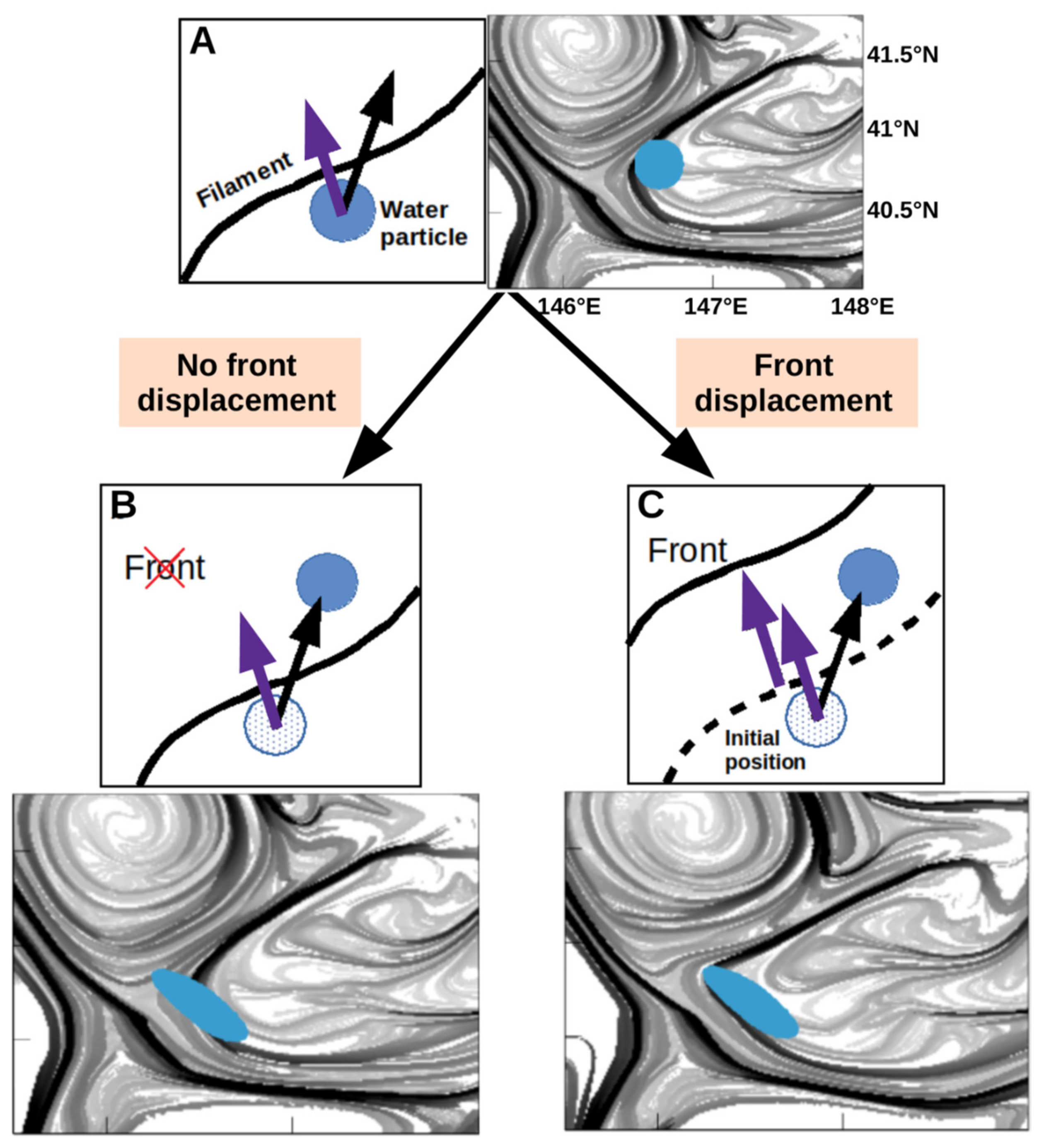
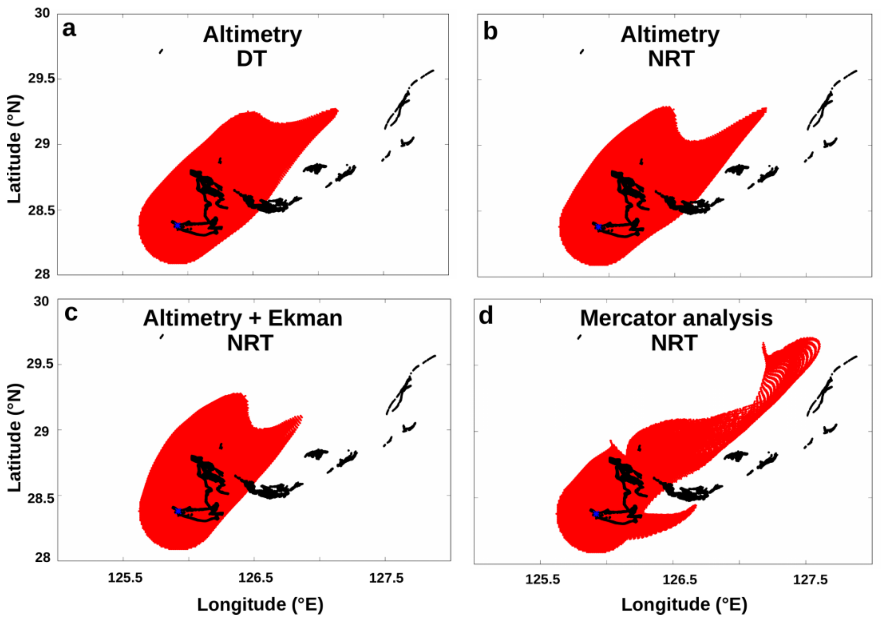

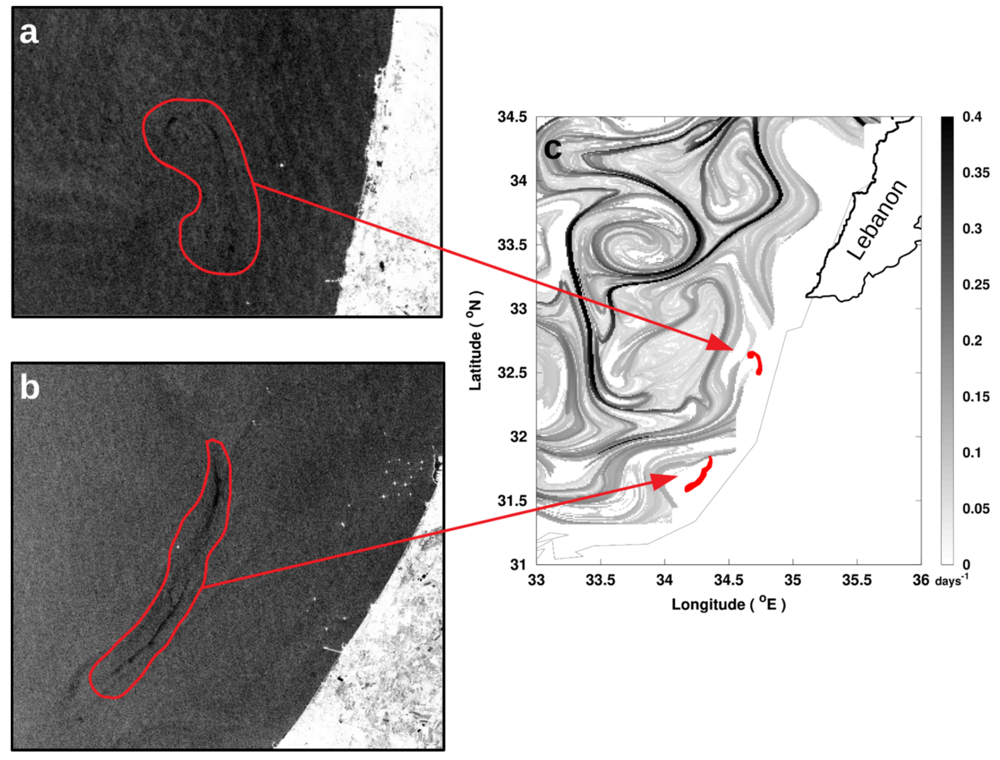

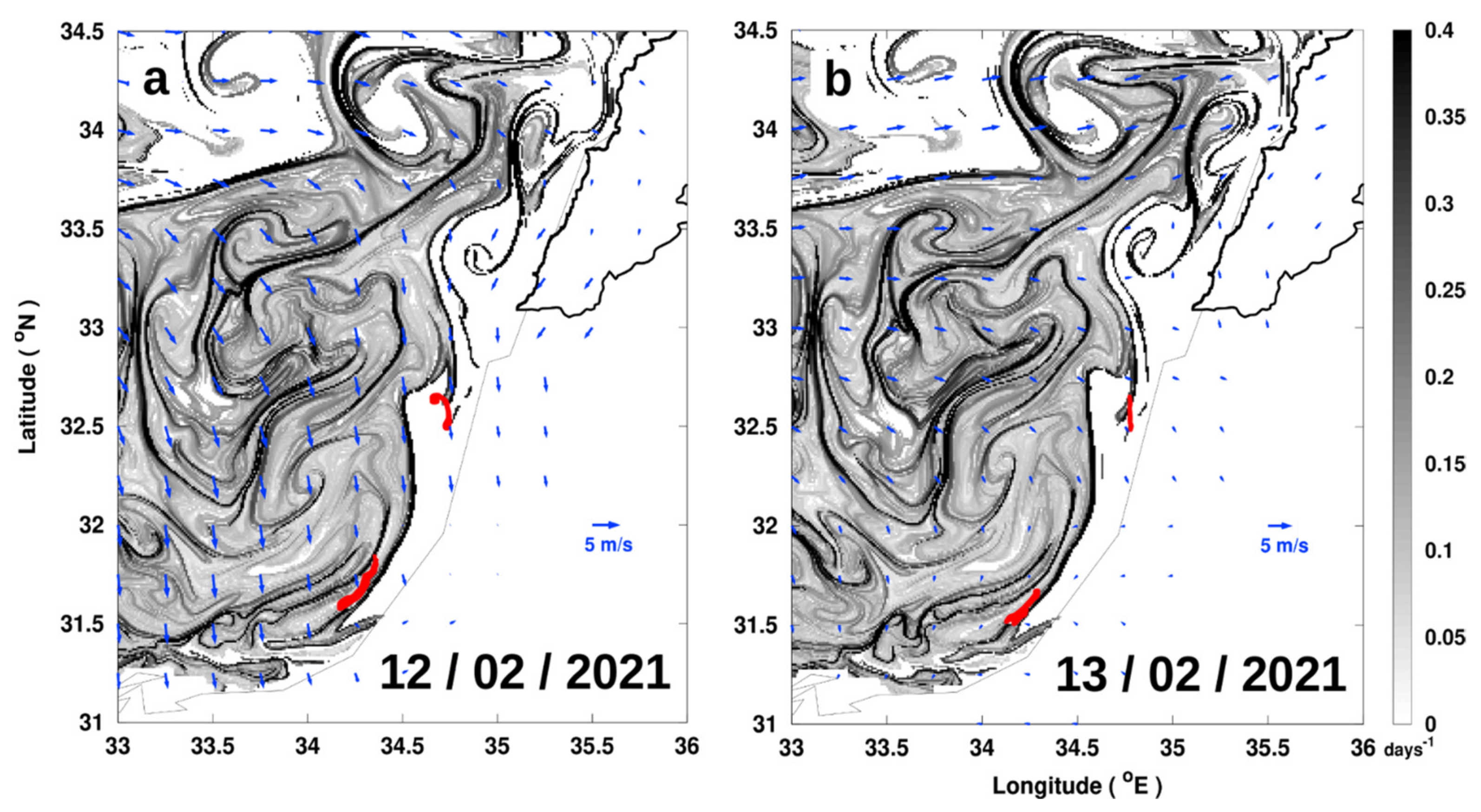
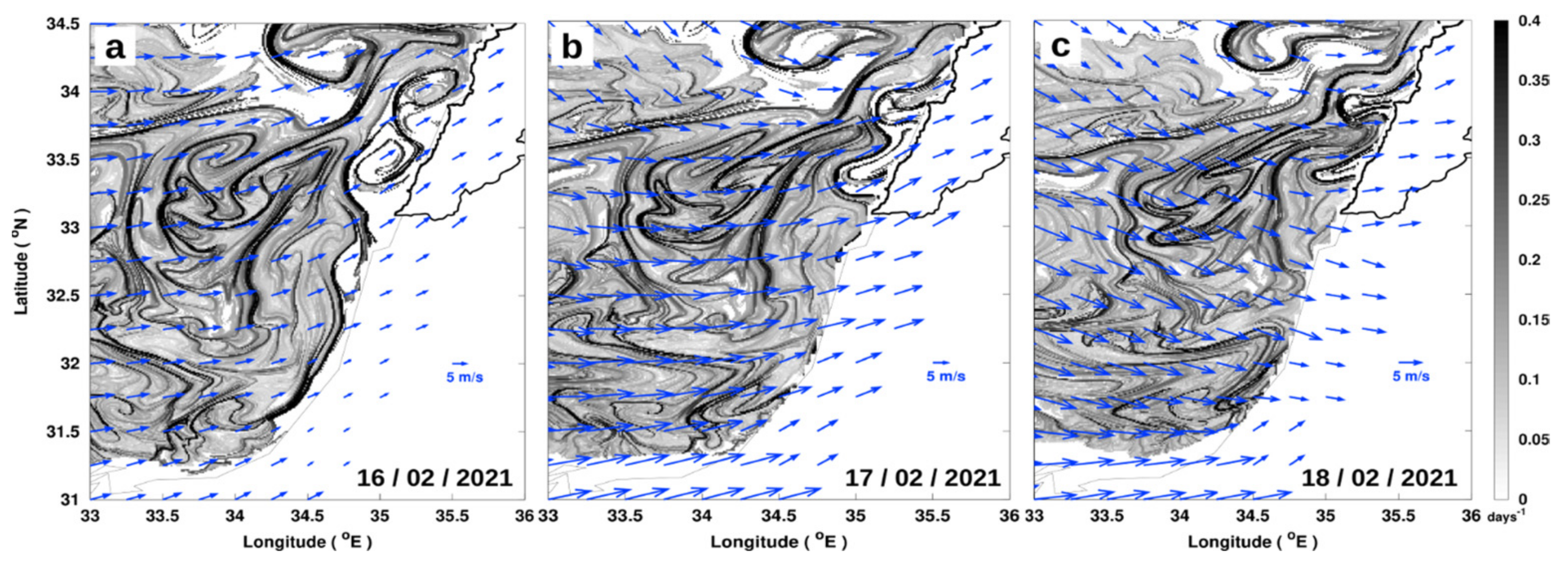
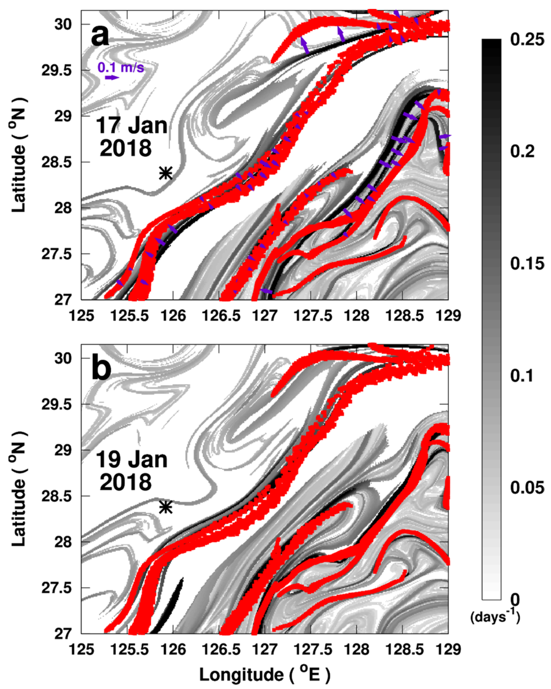
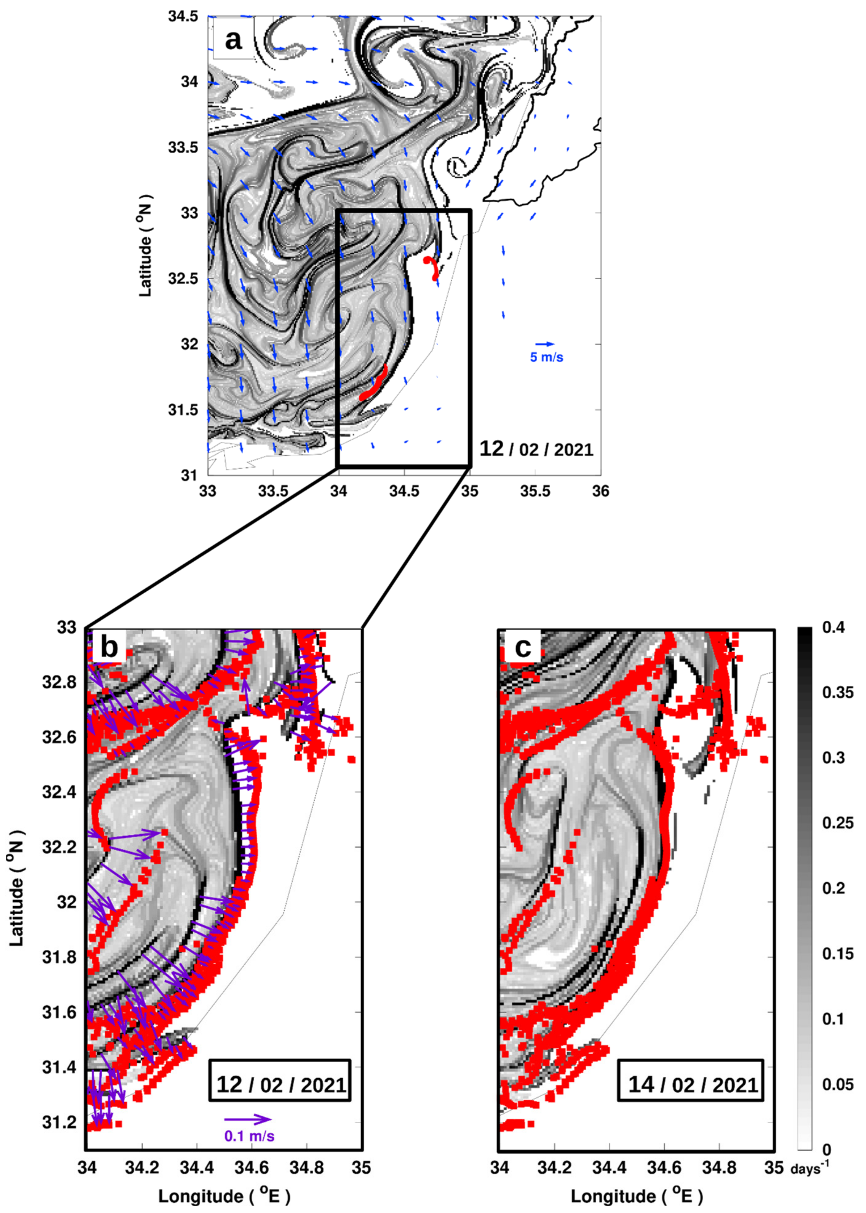
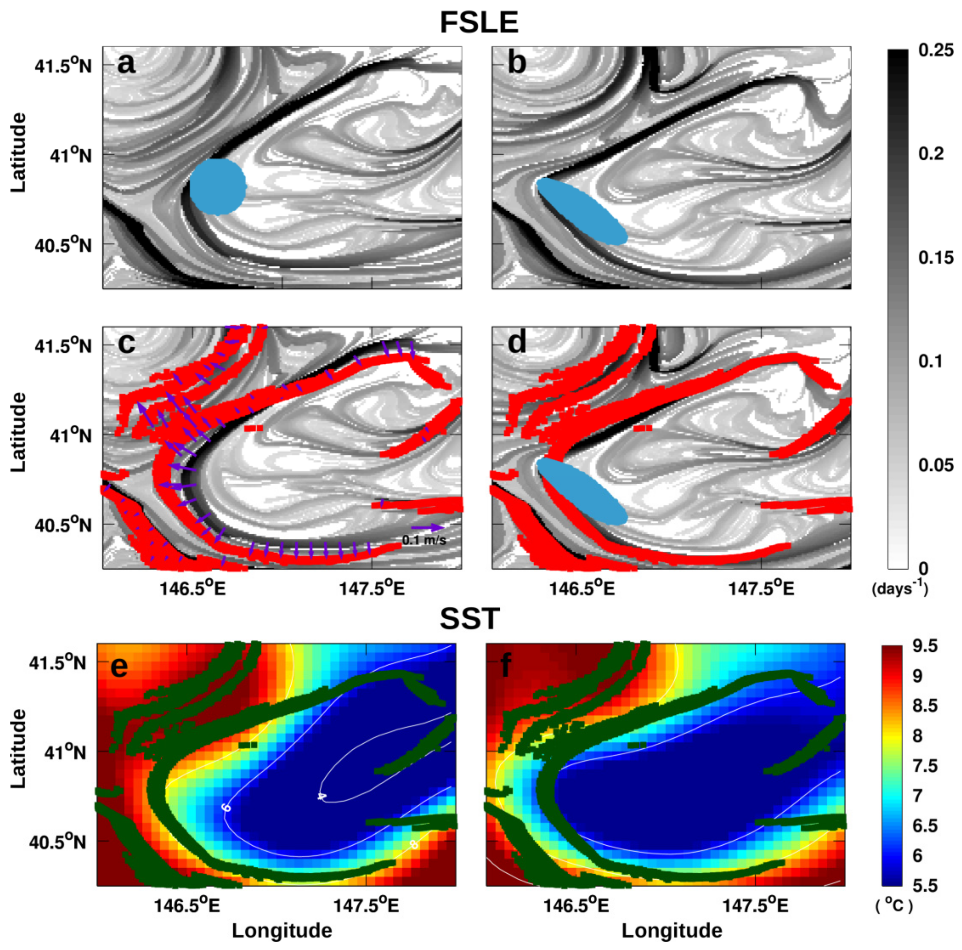
Publisher’s Note: MDPI stays neutral with regard to jurisdictional claims in published maps and institutional affiliations. |
© 2021 by the authors. Licensee MDPI, Basel, Switzerland. This article is an open access article distributed under the terms and conditions of the Creative Commons Attribution (CC BY) license (https://creativecommons.org/licenses/by/4.0/).