Monitoring and Forecasting of Urban Expansion Using Machine Learning-Based Techniques and Remotely Sensed Data: A Case Study of Gharbia Governorate, Egypt

Abstract

Rapid population growth is the main driver of the accelerating urban sprawl into agricultural lands in Egypt. This is particularly obvious in governorates where there is no desert backyard (e.g., Gharbia) for urban expansion. This work presents an overview of machine learning-based and state-of-the-art remote sensing products and methodologies to address the issue of random urban expansion, which negatively impacts environmental sustainability. The study aims (1) to investigate the land-use/land-cover (LULC) changes over the past 27 years, and to simulate the future LULC dynamics over Gharbia; and (2) to produce an Urbanization Risk Map in order for the decision-makers to be informed of the districts with priority for sustainable planning. Time-series Landsat images were utilized to analyze the historical LULC change between 1991 and 2018, and to predict the LULC change by 2033 and 2048 based on a logistic regression–Markov chain model. The results show that there is a rapid urbanization trend corresponding to a diminution of the agricultural land. The agricultural sector represented 91.2% of the total land area in 1991, which was reduced to 83.7% in 2018. The built-up area exhibited a similar (but reversed) pattern. The results further reveal that the observed LULC dynamics will continue in a like manner in the future, confirming a remarkable urban sprawl over the agricultural land from 2018 to 2048. The cultivated land changes have a strong negative correlation with the built-up cover changes (the R² were 0.73 in 1991–2003, and 0.99 in 2003–2018, respectively). Based on the Fuzzy TOPSIS technique, Mahalla Kubra and Tanta are the districts which were most susceptible to the undesirable environmental and socioeconomic impacts of the persistent urbanization. Such an unplanned loss of the fertile agricultural lands of the Nile Delta could negatively influence the production of premium agricultural crops for the local market and export. This study is substantial for the understanding of future trends of LULC changes, and for the proposal of alternative policies to reduce urban sprawl on fertile agricultural lands.

1. Introduction

The world is urbanizing rapidly; the urban covering is extending at twice the rate of population increase worldwide [1]. The superpower of urban convergence helps boost scientific and technological progress, and cultural exchanges. However, with the emergence of inequality in the division of wealth, this accelerated development is causing many sustainability challenges in terms of securing environmental sustainability, resource management, and the wellbeing of urban residents [2], e.g., biodiversity loss, increasing emissions of greenhouse gas, water scarcity, and environmental pollution [1,3]. Furthermore, many systems—such as transportation, housing, employment, privacy, and public morals—face enormous pressures and challenges, thus further negatively affecting human life [4,5]. The consequences of urban growth are most critical in developing countries, where urbanization is prominent and frequently random [6]. Therefore, the focus on urban studies and the development of research plans has become an urgent issue.

The regular and timely monitoring and mapping of human settlements at multiple spatial scales, from the local to the global, is critical to the realization of the spatial and temporal variability of population distribution and fresh urbanization trends, and to support global scopes such as the 2030 Agenda for Sustainable Development [7,8]. Many previous studies addressed the issue of urban sprawl by adopting different methodologies, e.g., Ranagalage et al. [9] examined and forecasted land-use changes in the rapidly urbanizing hill station of Nuwara Eliya, Sri Lanka, based on a neural network–Markov model. The findings show that the changes in cultivated land indicate a strong negative relationship with the changes in built-up cover along the urban expansion. Furthermore, Rimal et al. [10] addressed the study area of Nepal’s Terai region; a densely populated area that witnessed land-use changes owing to urban development. They utilized Landsat satellite images to examine past land-use change, highlighting urban growth and predicting its future trends using ANN and MC spatial models based on historical trends. Urban cover quadrupled over a 27-year period, and this expansion was roughly totally at the expense of agricultural diminution. The urban sprawl is predicted to continue according to the same trend over that study area.

Otherwise, our study focused on the areas suffering from accelerating urban sprawl on agricultural lands, resulting in food security challenges. In Egypt, the rapid population growth and growing demand for urban lands are the main drivers of the accelerating urban sprawl [11] into agricultural and arable lands. This is particularly obvious in the governorates that do not have a desert backyard. Gharbia governorate is a vivid example of a densely populated area (which experienced rapid urban growth over recent decades) where there is no desert backyard that could allow urbanization [12]. The main reason for the amplification of the problem of urban expansion in Egypt is that about 96% of the entire land area is unpopulated desert [13]. As such, the population is intensified completely in the Nile valley and the Delta. This unbalanced allocation and the massive rise in population led to critical socio-economic problems [2,14]. On the other hand, agriculture is a basic economic resource for Egypt [15], such that the diminution of agricultural land is one of the most important challenges facing agricultural development to achieve food security and agricultural rural stability. Even the reclamation of desert lands (new lands) cannot compensate for the deduction from the old lands in the short term due to the lower fertility of the new lands and the cost of the reclamation process. Therefore, the lack of agricultural production is a major problem for society in terms not only of the consumption of large amounts of foreign currency to fill the food gap resulting from the deduction of these areas but also the loss of products destined for export and the local markets for which the study area is famous, e.g., Egyptian cotton. Accordingly, understanding the dynamics of urban expansion and the motives behind the transgressions in such governorates, like Gharbia, is pivotal to promote sustainable land-use planning. This paper affords a survey of machine learning-based and state-of-the-art remote sensing-based products and methodologies that address the urban expansion over the agricultural and arable lands, and mapping of the transitional zones.

Furthermore, in order to make this study more productive, we employed Fuzzy TOPSIS to determine the level of susceptibility, for each district in the study area, to the urbanization risk in order for the decision-makers to be given the districts with priority for sustainable planning. As clarified, all of the previously mentioned studies focused on monitoring and forecasting the urban expansion over the different study areas, adopting different methodologies and achieving highly accurate and trustworthy results. However, what about the data-gap regions? If the area of interest is not covered by the satellite images, Fuzzy TOPSIS can be employed to evaluate the districts’ susceptibility to the urbanization risk.

Geodata science and spatial analysis are powerful for studying and monitoring land-use/land-cover change (LULCC), and for creating models for potential scenarios, being a substantial tool for management and decision-making to guarantee optimal land use [16]. These techniques have made major advances thanks to the availability of Remote Sensing (RS) images, sensors and Internet of Things (IoT) data; multi-source geospatial data; and new methods that have emerged, such as artificial intelligence (AI), particularly in its application to Earth observation (EO) [17]. RS imagery can efficiently capture the updated LULC allocation spatially and temporally [18], from which trends of LULC dynamics can be derived, analysed, and predicted [19]. Moreover, machine learning algorithms are a common subset of AI. Using machine learning algorithms can train data for predictive analysis, which leads to greater accuracy in the results [17,18,19,20]. Machine learning can be highly successful in image analysis tasks, involving land-use classification, simulation, and predictive analysis [21].

For land-use classification, a Support Vector Machine (SVM) is one of the most common machine learning image classifiers [22,23,24,25]. An SVM was considered in this study to extract LULC from Landsat images because it can handle overlapping classifications [24,25]. It outperforms other algorithms when there are large features and fewer training data. Moreover, it presents a notably higher classification accuracy and classification speed than other algorithms [26], as confirmed by Yousefi et al. [27].

For simulation, there are diverse modeling methods capable of simulating and predicting LULC, including SLEUTH [28], and the Conversion of Land Use and its Effect (CLUE) [29]. The SLEUTH model, for example, simulates LULC variation in the future based on land-use behavioral change [30], whereas CLUE simulates spatio-temporal LULCC as a result of human and biophysical drivers. The Markov chain (MC) algorithm completes such spatial models of LULCC by a stochastic estimate of land-change transition potential without determining the spatial extent of such transitions [31,32]. Consequently, because spatial models such as cellular automata (CA) concentrate specifically on the land-change transitions spatially, usually based on past trends, a hybrid model that includes MC can estimate the location and quantification of conversions relying on historical LULC trends [33]. The logistic regression–Markov chain model is one of the superior hybrid models for the estimation of future land change transitions [33,34,35]. A substantial advantage is clear when compared with different models such as CA, which requires transfer rules to manage change procedures, or the SLEUTH model, which requires the parameter values to be known in advance. The logistic regression–Markov chain model was utilized to simulate LULC changes in Aswan, Egypt [34]; Tehran, Iran [33]; and Giao Thuy District, Vietnam [35]. The integration of MC (with superior potential for transition estimation) [36] and logistic regression as a spatial model (which focuses on the location of land-change transitions, usually based on archival trends) assists in the generation of transition probability maps [37].

The identification of spatiotemporal patterns of LULCC and regarding driving forces is necessary to promote perfect urban strategies and policies which can guarantee economic, social, and environmental sustainability [15]. Therefore, this study includes three principal objectives: (1) to investigate the LULC dynamics over the past 27 years, (2) to simulate the future LULCC for 2033 and 2048 in the Gharbia governorate, and (3) to produce an Urbanization Risk Map illustrating the susceptibility level to the urbanization risk. The study focuses on promoting the capability and understanding of policymakers and the local government to reduce the potential undesirable effects of rapid urban growth inside the study area.

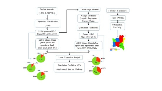
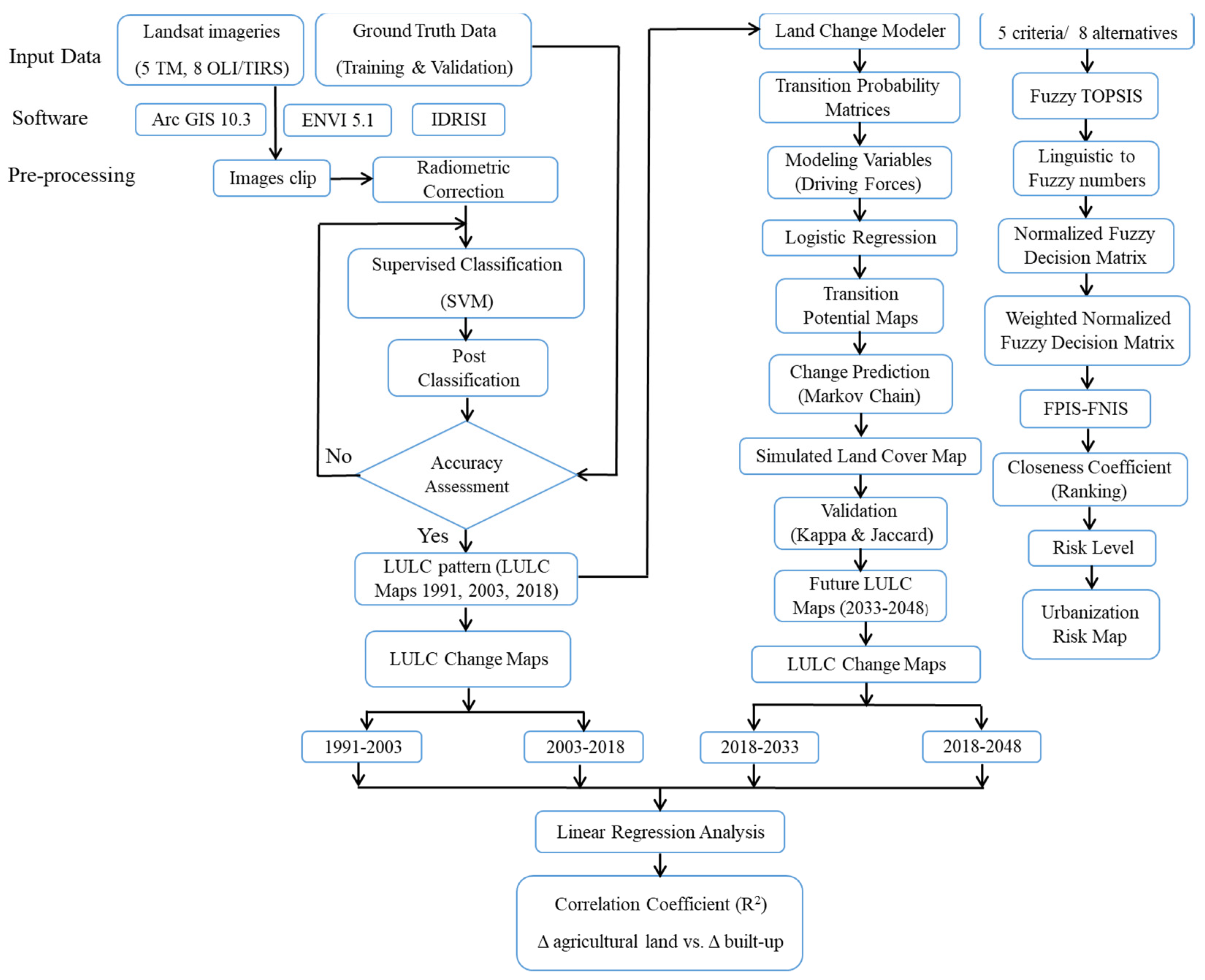
2. Materials and Methods

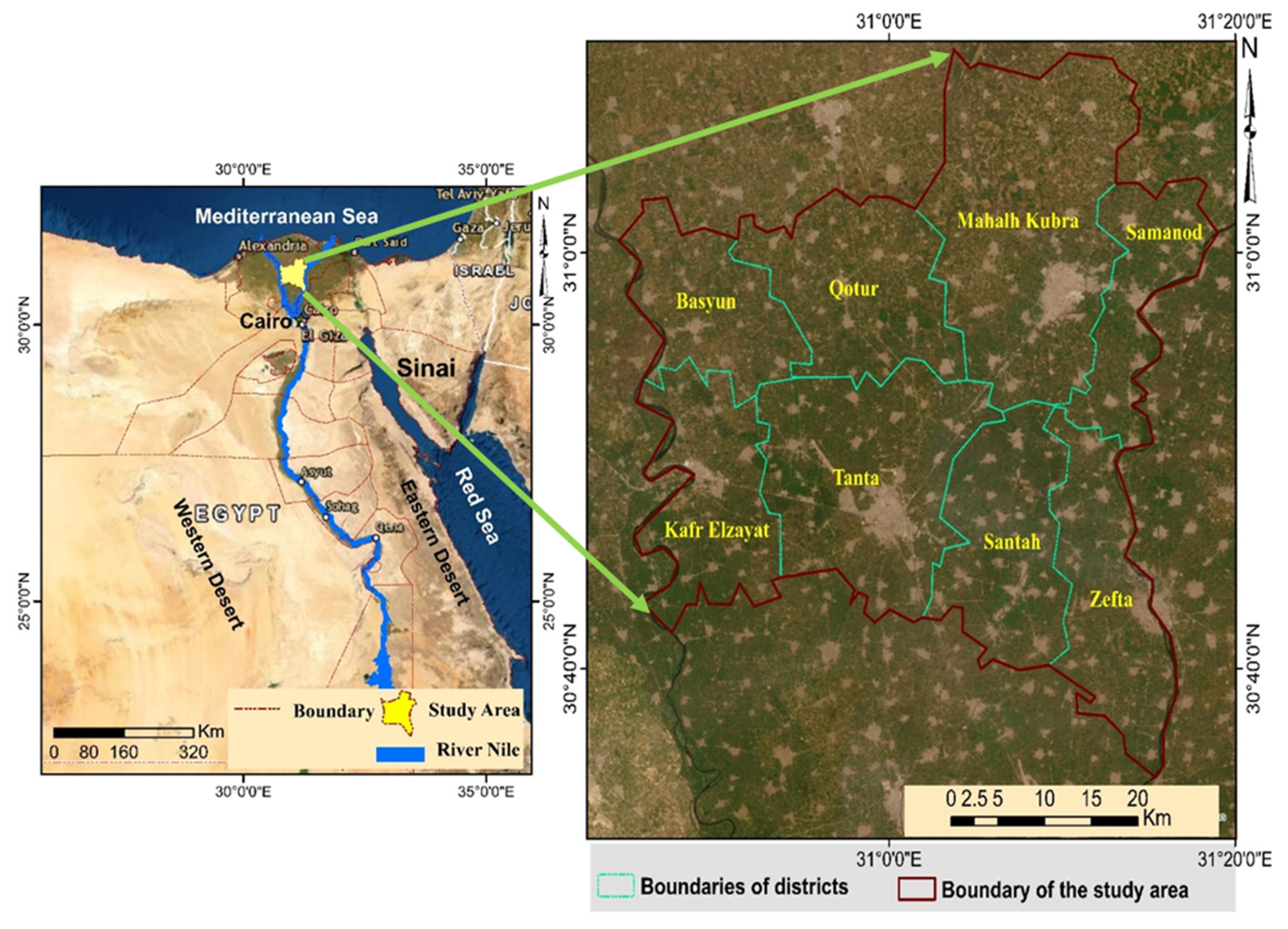
2.1. Study Area

Gharbia governorate is located in the heart of the Nile Delta of Egypt, at 30.87° N latitude and 31.03° E longitude. It is bordered to the north by Kafr El-Sheikh governorate, to the south by Monufia governorate, and to the east and west, respectively, by the Damietta and Rosetta branches of the Nile. The Nile Delta is one of the most ancient agricultural areas worldwide. It has been ceaselessly cultivated for more than 5000 years [2,38]. The Nile River provided the Delta soil with natural fertilizers and therefore high agricultural production, creating an obvious green triangular region within a wide desert. The agricultural land as a LULC category is dominant in the governorate, which is famous for the cultivation of traditional crops, e.g., potatoes for the local market and export, in addition to the rice, grains, and cotton which is famous for its superior quality. Moreover, this governorate produces 86% of the flax crop in Egypt. Gharbia consists of eight districts, as shown in Figure 1. According to the population estimate of 2018, there are about 5,066,000 people residing in a total land area of 1999 km². Otherwise, the population was only 4,011,320 and 3,790,670 in 2006 and 2001, respectively.

2.2. Data Collection and Processing

This study employed time-series Landsat imageries gained from the United States Geological Survey (USGS) website. They were relied upon because of their rich and free archive that allows long-term study. The Landsat 5 Thematic Mapper (TM) and Landsat 8 OLI/TIRS were used to obtain LULC maps [39] for 1991, 2003, and 2018, and to extract the land-cover changes over the years [40]. The obtained images were pure, with no cloud shades thanks to the dry summer season. The three images were atmospherically corrected. Before the image analysis, all of the scenes were stacked and put into subsets by the region of interest. The study area is located in two successive scenes, so a mosaic was employed. This paper has a further research area concerning the impact of LULCC on the land surface temperature over this study area. Therefore, it was preferred to select the images in the same season for a more realistic comparison over the years. However, if we only address the LULCC, there is no need to consider the capture date of the images for the different years. The road network gained from the open street map (OSM) was used as auxiliary data to extract the layer of “distance to the nearest road”, which will be used later. Moreover, the training samples used for the supervised classification process and its validation were also acquired based on Google Earth Pro as mentioned in

Table 1. Description of the data used.

Data Type	Capture Date	Resolution	Source	Output
Landsat 1991TM	27 June 1991	30 m	USGS	LULC map
Landsat 2003TM	28 June 2003	30 m	USGS	LULC map
Landsat 2018OLI-TIRS	21 June 2018	30 m	USGS	LULC map
Training Samples			Google Earth Pro	Training/Validation
Road Network layer			OSM	Distance to nearest road

.

Figure 2 illustrates the conceptual flowchart of the applied methodology to fulfill the aforementioned objectives with five fundamental steps: (1) the extraction of LULC maps from multi-temporal Landsat images [41] using a machine learning algorithm for classification [42], followed by post-classification to limit the misclassification errors or salt and pepper noises caused by spectral confusion [43], and the evaluation of the accuracy of the classification process so that the change detection can be relied upon [44]; (2) choosing the most appropriate modeling variables which are the driving forces of the LULCC (representing the urban sprawl parameters) [45] and obtaining transition potential maps [34] illustrating the transition between the land-use types; (3) LULCC simulation/validation and future projection based on the Land Change Modeler (LCM) [46,47], adopting a logistic regression algorithm and the Markov chain model, followed by the validation of the simulation process to test the model’s capability of prediction; (4) linear regression analysis is employed to investigate the correlation between the changes in different land-use types; and (5) applying a multi-criteria decision-making (MCDM) technique (Fuzzy TOPSIS) to determine the level of the susceptibility of the districts to the urbanization risk in the form of an Urbanization Risk Map [48], especially in the absence of satellite images.

2.3. LULC Classification

As visually interpreted through the used data images, the study area has only 3 LULC classes: built-up, water, and agricultural land. We relied on a pixel-based supervised classification method which is appropriate to the primary data used, which are themselves labeled as medium-resolution data (i.e., Landsat images). We depended on two classification techniques: Maximum Likelihood Classification (MLC) as a parametric pixel-based method, and SVM classification as a non-parametric pixel-based approach. However, even visually, the SVM-based classified image simulated the actual categories much better than the MLC technique. This is because SVM is a kernel-based algorithm that starts working with data in a relatively low dimension and then moves them into a relatively high dimensional space, finding a relatively high dimensional support vector classifier that can effectively classify the observations [49,50]. Subsequently, SVM was considered to extract LULC from Landsat images.

There was some misclassification in the first results of the classification process. This is why the majority filter was adopted in the post-classification to limit the misclassification errors or salt and pepper noises caused by spectral confusion [43,51]. In other words, the post-classification improvement is a successful technique to considerably upgrade the results’ accuracy.

2.4. Accuracy Assessment

So as to verify whether the classification results are accurate for change detection, a quantitative accuracy evaluation was performed. The most common technique to assess the accuracy of land cover maps is the confusion matrix [52,53]. The confusion matrix contrasts a classified image with its corresponding reference image on a category-by-category basis. The samples required for the training of all of the classes, in addition to those for validation, were obtained based on Google Earth historical images. We used a random sampling method [54,55] to generate 1000 checkpoints for each image, which covered all of the LULC classes and were well distributed, in order to obtain more realistic classification accuracy [54]. Based on the error matrix, the Overall Accuracy (OA%) was used to express the classification accuracy assessment. However, OA doesn’t detect whether the error was evenly distributed between the classes, or if some classes were really bad and others were really good. Therefore, three indices of accuracy were also computed: User’s Accuracy (%), Producer’s Accuracy (%), and the Kappa coefficient [56,57].

2.5. LULC Change Modeling

The land change modeling process involves three main steps: (1) model calibration, (2) model simulation and validation, and (3) model projection. Before the model calibration, the preparation of the data is required; the land cover images must have the same extent, projection, background areas and values, and legends. These steps were performed via LCM [58,59]. The LCM is integrated into the TerrSet Geospatial Monitoring and Modeling System software (Clarke Labs 2019 [60]), which is efficient at LULCC analysis, simulation and validation, and future projection [46]. The land change analysis is the exploration of the land change dynamics between two points of time. LCM provides a superior perception of LULCC patterns to support urban planning and sustainable development [46].

2.5.1. Model Calibration (1991–2003)

The model was calibrated for pixels that changed from each LULC class to other classes between 1991 and 2003. The “transition potentials” for each modeled transition were determined using an MC stochastic model [61], whereas a sub-model representing the transition potentials to the built-up area was specified using the logistic regression. Combining the MC approach—which has been popularly adopted to predict LULC distribution with spatial models, involving MLP-ANN, CA, and logistic regression models [62,63]—was recommended. A hybrid model of MC and logistic regression can gather the advantages of both the quantification and determination of the spatial extent of the conversion states among the different LULC types [31].

The selection of the most appropriate modeling variables for the sub-model is one of the significant steps in LULC modeling. These variables are the driving forces of the LULC dynamics when conducting spatiotemporal prediction [64,65]. For instance, in order to monitor urban growth, urban sprawl parameters have to be taken into account. According to previous studies related to the modeling of land change and urbanization [9,66], as well as the available data, some common driving forces of the LULCC—particularly when predicting the anthropogenic activities —include:

a.

The distance from roads: Roads can provide access to previously remote areas promoting urbanization near roadways.

b.

The distance from urban centers: Urban centers tend to grow and expand as the human population increases, such that the areas surrounding current urban centers are frequently susceptible to land change.

c.

The distance from persistent built-up areas: Areas that have already been disturbed by humans often have the infrastructure in place to promote further urbanization along current persistent built-up edges.

d.

The distance from railway stations: This is the same effect of the driver of “distance from roads”.

e.

Digital Elevation Model (DEM): Because of the environmental gradient, characteristics such as temperature and rainfall alter with elevation; elevation is a proper indicator of areas that are appropriate for cultivation (and thus are prone to transition to agricultural land) and for subsequent development (for instance, the lowland area is more disposed to evolution).

f.

Slope: The slope is the principal of determining whether the land is advantageous to humans. For example, agriculture and building require fairly gentle slopes, such that areas with these slopes may be more likely to experience land cover change.

Previous studies have confirmed that the fittest way to choose the variables depends on the properties of the study area, the detected LULCC overtime, and the expert familiarity with the different study areas [67,68]. Therefore, based on our knowledge of the study area, considering the development pattern of the area, we adopted four modeling variables (the aforementioned a, b, c and d, as shown in Figure 3) as driving forces of the LULCC in the study area. The DEM and slope can be neglected, as the study area is almost level. All of the distance-based variables were generated by the Euclidean distance method. After the variable extraction, a standardization technique was applied for the rescaling of the four variables between 0 and 1 (as the logistic regression, as a machine learning algorithm, always adopts), for the minimization of the self-impact of the variables having diverse ranges. Then, the logistic regression algorithm was applied to produce transition potential maps depicting the probability of each conversion at a specified location in the whole study area.

2.5.2. LULC Simulation and Model Validation (2003–2018)

After the calibration of the model, we simulated the LULC of 2018 based on the trends noticed during the calibration period (1991–2003). Then, the simulated 2018 LULC map was compared with the observed 2018 LULC map produced earlier based on the SVM supervised classification of the Landsat image, in order to validate the model. The model validation was used to evaluate how effective the LCM is in simulating and then extrapolating the future LULC maps [69,70]. The model outputs the Cohen’s Kappa coefficient [71] as an indicator of the degree of the matching between the simulated and observed 2018 LULC maps. The values of Kappa of 0 to 0.2 point out the slight relationship between the two maps, while the values of 0.81 to 1 are a nearly ideal agreement [72,73].

As the Kappa index may not be enough to assess the simulation potential properly [74], the Jaccard similarity coefficient was used to cross-check the results [75]. The Jaccard coefficient is used to characterize the performance of a model for the proper simulation of LULCC. It is defined as the ratio of properly simulated change area versus the entire area of properly and improperly simulated LULCC or constancy [76]. In other words, it is defined as the area of intersection between the two layers (simulated and actual) divided by their union area, as shown in Equation (1). It ranges from 0% to 100%, indicating the degree of agreement between the actual and simulated change, where 0% means no intersection between the two layers and 100% means perfect intersection. Because the remarkably observed transition was represented in the urban sprawl over the agricultural land, the observed and simulated built-up layer for 2018 was extracted, and then the Jaccard coefficient was derived.

$$J_c\left(simulated,observed\right)2018=\frac{simulated urbanization\cap \mathit{observed}\mathit{urbanization}}{simulated urbanization\cup observed urbanization}$$

(1)

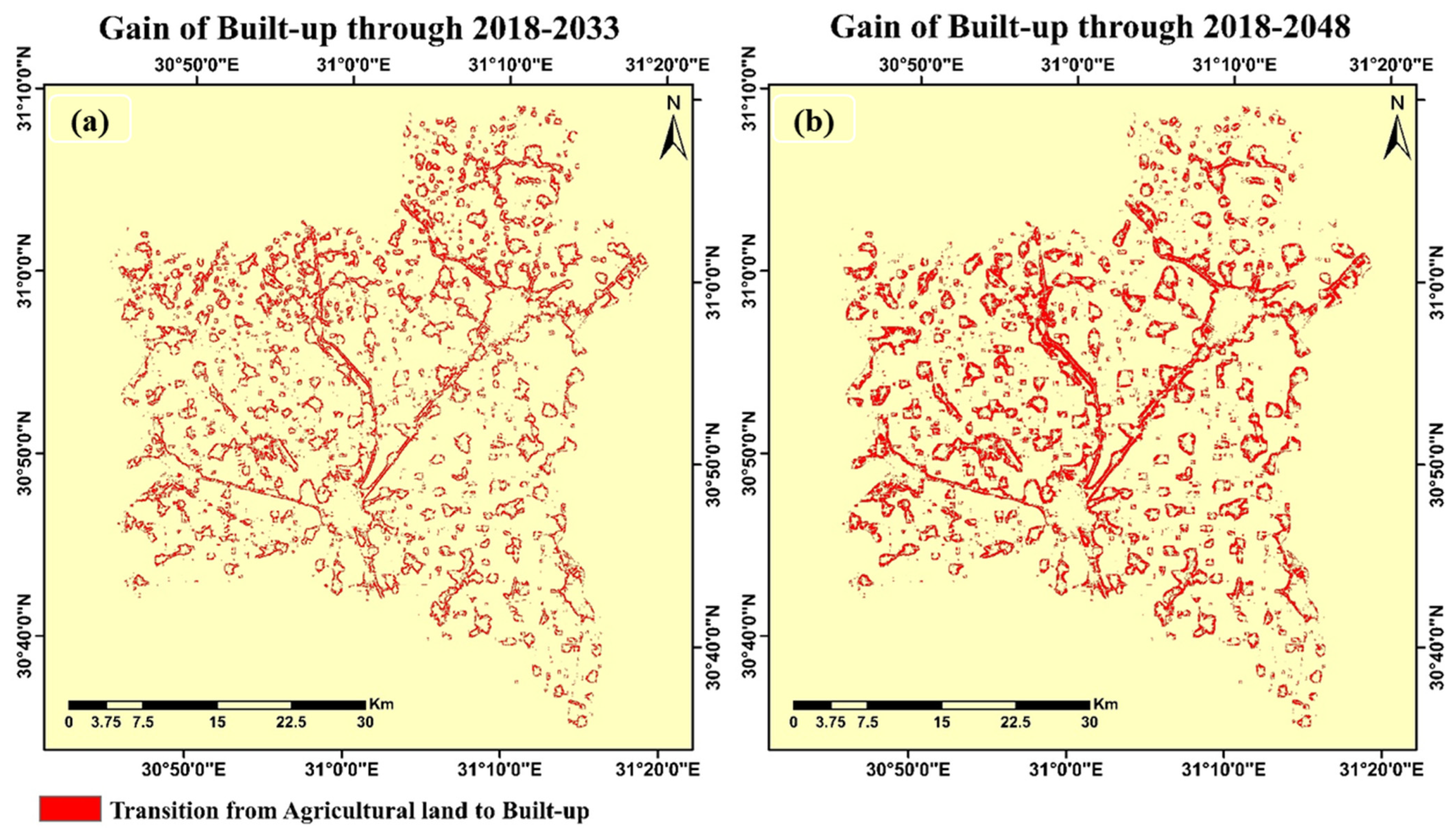
2.5.3. Projecting Future LULC Changes (2018–2033/2048)

Subsequent to the model calibration and validation, the final step is the projection of the LULCC forward to 2033 and then to 2048 using the MC, producing two LULC maps for these future dates. The projected rates of LULC were extrapolated from the simulation period (2003–2018). Furthermore, the modeling variables (the driving forces of LULCC) were first updated to 2018 before running the prediction. For instance, the “Distance from persistent built-up areas” would be updated for the period 2003–2018. Furthermore, the observed LULC of 2018 (not the simulated one) would be used in the new session of LCM to project the future LULC in 2033 and 2048.

2.6. Fuzzy TOPSIS Analysis

The Fuzzy TOPSIS (Technique for Order Preference by Similarities to Ideal Solution) is an MCDM technique, which was originally stated by Hwang and Yoon in 1981, with additional developments by Yoon in 1987, and Hwang, Lai and Liu in 1993 [77]. TOPSIS relies on the concept that the preferred alternative should have the shortest geometric distance from the positive ideal solution (PIS) and the longest geometric distance from the negative ideal solution (NIS) [48]. In order to avoid uncertainty in the data and analysis, a fuzzy technique was employed. Utilizing fuzzy numbers in TOPSIS for criteria analysis makes it easy to evaluate. The used fuzzy numbers were extracted based on the triangular membership function [78,79]. Gharbia governorate has eight urban centers, and we need to monitor the trend of urban growth through these centers to assist in producing an Urbanization Risk Map. We have applied Fuzzy TOPSIS for the determination of the district which is the most susceptible to urbanization risk, and thus has the priority to be considered by the decision-makers. The following are the steps of applying the Fuzzy TOPSIS method [48] (A spreadsheet of the numerical matrices has been inserted in the Supplementary Materials):

• Step 1: Alternatives rating by decision-makers and applying for fuzzy numbers.

Here, we have eight alternatives (representing the eight districts of the study area) for the decision, based on five criteria by which the regions could be judged in terms of the level of risk, including population growth, employment, local development, area, and socio-economic conditions. The criteria data for each alternative were obtained based on the government reports released on social media. Conversion metrics were applied to convert the linguistic terms into fuzzy numbers. Typically, a scale of 1 to 9 is applied to rank the criteria and alternatives. The intervals are selected to have a uniform representation from 1 to 9 for the fuzzy triangular numbers utilized for the five linguistic evaluations.

Table 2. Fuzzy rating for linguistic terms.

Linguistic Term	Fuzzy Number
Very high	7, 9, 9
High	5, 7, 9
Moderate	3, 5, 7
Low	1, 3, 5
Very low	1, 1, 3

illustrates the fuzzy rating for the linguistic terms. The Combined Fuzzy Decision Matrix of the criteria and alternatives (shown in

Table 3. The Combined Fuzzy Decision Matrix of the criteria and alternatives.

Weightage	7, 9, 9	7, 9, 9	5, 7, 9	5, 7, 9	3, 5, 7
Criteria Alternatives	Population Growth	Employment	Local Development	Area	Socio-Economic Conditions
Mahalla Kubra	7, 9, 9	7, 9, 9	5, 7, 9	7, 9, 9	5, 7, 9
Tanta	7, 9, 9	7, 9, 9	5, 7, 9	7, 9, 9	5, 7, 9
Basyun	1, 4, 7	1, 3, 5	1, 4, 7	3, 5, 7	1, 4, 7
Zefta	3, 6, 9	1, 4, 7	1, 4, 7	3, 5, 7	1, 3, 5
Santah	1, 4, 7	1, 4, 7	1, 4, 7	3, 5, 7	1, 4, 7
Kafr Elzayat	5, 7, 9	5, 7, 9	3, 5, 7	5, 7, 9	1, 4, 7
Samanod	1, 4, 7	1, 3, 5	3, 5, 7	3, 5, 7	1, 3, 5
Qotur	5, 7, 9	3, 5, 7	3, 5, 7	5, 7, 9	1, 4, 7

) was obtained from two fuzzy decision matrices, as we considered two decision-makers.

• Step 2: Normalizing the fuzzy decision matrix using Equation (2).

The fuzzy decision matrix has the ith alternative on the jth criterion, and the triangular fuzzy number is represented by (a_ij, b_ij, c_ij)

$$Ȓ={\left[{ȓ}_{ij}\right]}_{m*n}\mathrm{i}=1,2,...,\mathrm{m};\mathrm{j}=1,2,...,\mathrm{n}$$

where, Ȓ is the normalized fuzzy decision matrix:

$${ȓ}_{ij}=[\frac{a_{ij}}{c_j^{*}},\frac{b_{ij}}{c_j^{*}},\frac{c_{ij}}{c_j^{*}}]\mathrm{and}{c}_j^{*}=\underset{i}{max}\left\{c_{ij}\right\}\left(\mathrm{benefit}\mathrm{criteria}\right)$$

(2)

Note that each criterion is a benefit criterion. Furthermore, the normalized triangular fuzzy numbers range from 0 to 1.

• Step 3: Computing the weighted normalized fuzzy decision matrix using Equation (3).

$${\mathsf{Õ}}_{ij}={ȓ}_{ij}\times W_j$$

(3)

where W_j is the weight of each criterion (3).

• Step 4: Computing the Fuzzy Positive Ideal Solution (FPIS) using Equation (4) and the Fuzzy Negative Ideal Solution (FNIS) using Equation (5).

$$A^{*}=\left({\mathsf{Õ}}_1^{*},{\mathsf{Õ}}_2^{*}, ....,{\mathsf{Õ}}_n^{*}\right)\mathrm{where}{\mathsf{Õ}}_j^{*}=\underset{i}{\max }\left({\mathrm{O}}_{ij3}\right)\mathrm{i}=1,2,...,\mathrm{m};\mathrm{j}=1,2,...,\mathrm{n}$$

(4)

$$A^{-}=\left({\mathsf{Õ}}_1^{-},{\mathsf{Õ}}_2^{-}, ....,{\mathsf{Õ}}_n^{-}\right)\mathrm{where}{\mathsf{Õ}}_j^{-}=\underset{i}{\min }\left({\mathrm{O}}_{ij1}\right)\mathrm{i}=1,2,...,\mathrm{m};\mathrm{j}=1,2,...,\mathrm{n}$$

(5)

Select the maximum value from each row as Õ⁺, and select the minimum value from each row as Õ⁻.

• Step 5: Computing the distance from each alternative to the FPIS and to the FNIS using Equation (6).

$$d^{*}\left({\mathsf{Õ}}_{ij},A^{*}{}_j\right)=\sqrt{\frac{1}{3}[{(\Delta a)}^2+{(\Delta b)}^2+\left(\Delta c{)}^2\right]}$$

(6)

Do the same for $d^{-}\left({\mathsf{Õ}}_{ij},A^{-}{}_j\right)$, then compute the sum of the distances using Equations (7) and (8):

$$d^{*}{}_i={\displaystyle \sum }_{j=1}^{n}d\left({\mathsf{Õ}}_{ij},A^{*}{}_j\right)$$

(7)

$$d^{-}{}_i={\displaystyle \sum }_{j=1}^{n}d\left({\mathsf{Õ}}_{ij},A^{-}{}_j\right)$$

(8)

• Step 6: Compute the Closeness Coefficient (CCi) for each alternative using Equation (9).

$$C{C}_i=\frac{d_i^{-}}{d_i^{-}+d_i^{*}}$$

(9)

3. Results

3.1. Accuracy of the LULC Maps

The classification result revealed three classes throughout the study area: built-up, water, and agricultural land. The built-up class involved buildings, roads, and all other impervious surfaces. The previously mentioned four indices of accuracy are summarized in

Table 4. Classification accuracy assessment of the LULC types.

Accuracy	LULC Class	1991	2003	2018
User’s Accuracy (%)	Built-up	85.7	90.7	91.8
	Water	88.9	76.2	92.3
	Agricultural land	94.8	95.3	94.8
Producer’s Accuracy (%)	Built-up	67.8	78.5	83.1
	Water	64.0	66.7	54.5
	Agricultural land	98.3	97.9	98.1
Overall Accuracy (%)		93.9	94.3	94.3
Kappa Coefficient		0.73	0.79	0.82

for the three images of 1991, 2003, and 2018: the Overall Accuracy (%); the Kappa Coefficient for each classified image, in addition to User’s Accuracy (%); and the Producer’s Accuracy (%) for each land cover type. The error matrices upon which the accuracy indices were computed have been inserted in the Supplementary Materials (Tables S1–S3). As is visible in Table 4, each of the three classification dates attained satisfying overall accuracies of 93.9 %, 94.3% and 94.3%, and corresponding desired kappa coefficients of 0.82, 0.79 and 0.73 for 1991, 2003 and 2018, respectively. SVM confirmed high classification potential. However, there is some mutual misclassification in the water and irrigated agricultural land owing to the close spectral similarity between these two classes in a single temporal image. Therefore, the seasonal behavior of crops is an essential component of successful image interpretation.

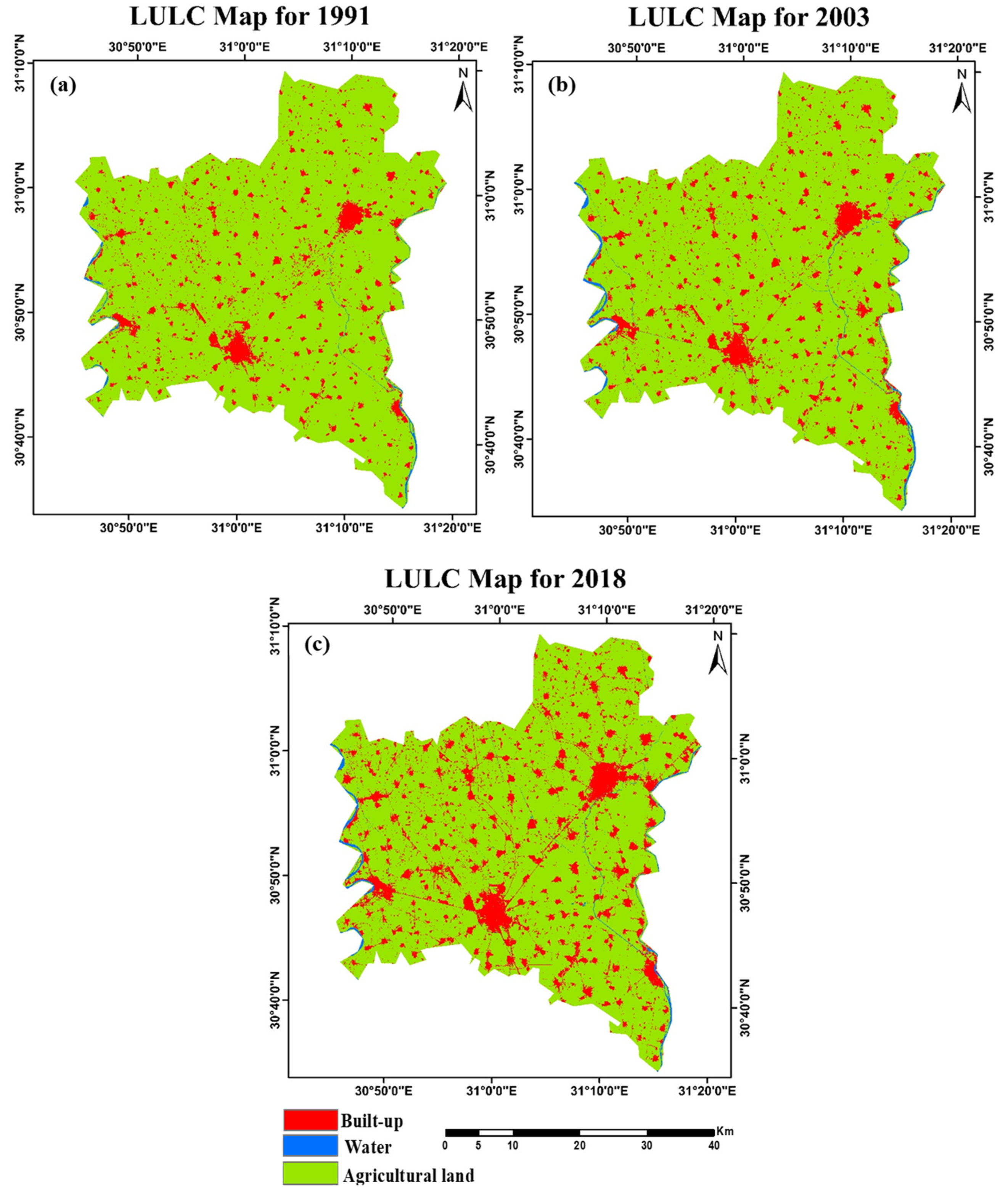
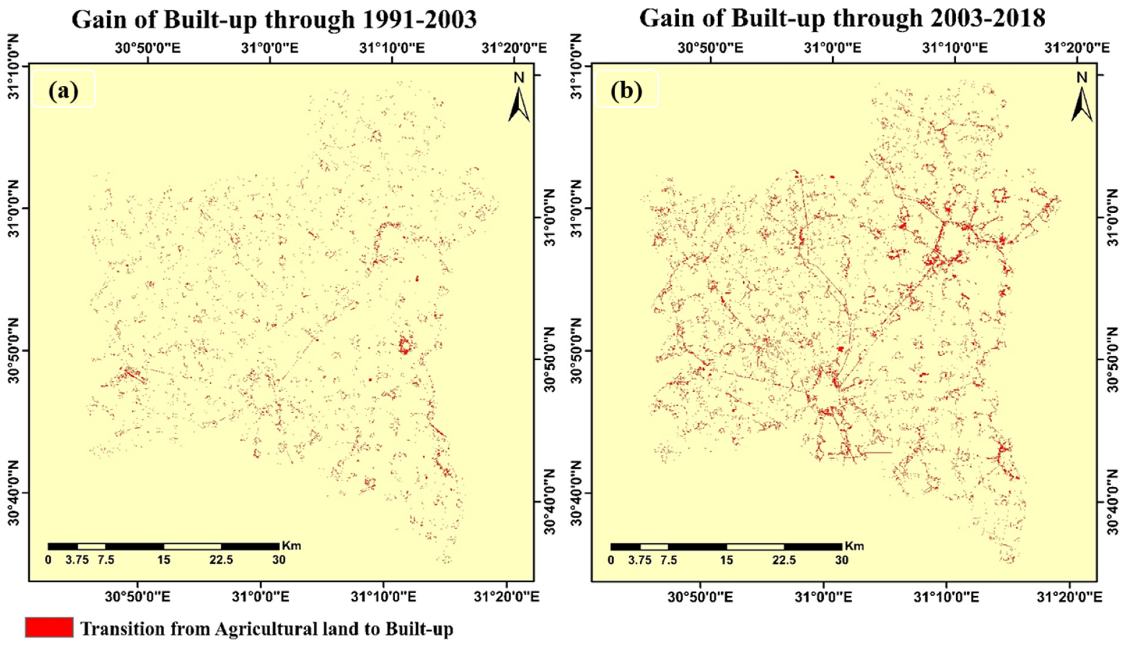
3.2. Spatiotemporal Analysis of LULCC

The classification and quantification of the images of the study area (illustrated in Figure 4 and summarized in

Table 5. Details of the LULCC in Gharbia governorate in 1991, 2003 and 2018.

LULC	1991		2003		2018
	Area (km2)	%	Area (km2)	%	Area (km2)	%
Built-up	156.75	7.8	193.37	9.7	303.75	15.2
Water	19.57	1.0	24.48	1.2	21.56	1.1
Agricultural land	1832.01	91.2	1781.48	89.1	1674.02	83.7
Total	1999.33	100	1999.33	100	1999.33	100

) are vital for LULCC detection within the study area and over the study period. LULC maps for 1991, 2003, and 2018 are illustrated in Figure 4a–c, respectively. Table 5 elaborates the area of each class over the different years in both squared kilometers and percentages. It was shown that the agricultural land was dominant, occupying 91.2% (representing 1832 km²) of the total land area in 1991; however, it was reduced to 83.7% (representing 1674 km²) in 2018. The water bodies filled the smallest area of about 1%, and stayed almost the same over the years. Statistical analysis of 2003 study year showed that there is was an increase in the built-up area at the expense of the agricultural land; however, this augment (around 2%) is not alarming. On the other hand, over the period of 2003–2018, the urban growth continued, looking forward to urbanization, and experienced considerable augmentation (around 5.5% of the total area), where the built-up area represented 9.7% and 15.2% in 2003 and 2018, respectively. The urban growth over the agricultural land which represented the LULCC over the time periods of 1991–2003 and 2003–2018 is demonstrated in Figure 5a,b, respectively.

LULCC analysis can also be performed in another way, by computing the Relative Deviation (RD) of different land-use categories from the year 1991 to 2003, 2003 to 2018, and 1991 to 2018 (as mentioned in

Table 6. Relative Deviation (RD %) for each class through the three time periods (1991–2003, 2003–2018, and 1991–2018).

RD %	1991–2003	2003–2018	1991–2018
Built-up	+23.4	+57.1	+93.8
Water	+25.1	−11.9	+10.2
Agricultural land	−2.8	−6.0	−8.6

) using Equation (10).

$$\%\mathrm{RD}=\frac{\mathrm{A}-\mathrm{B}}{\mathrm{B}}\times 100$$

(10)

where A is the area under a specified land-use class for the second (new) year, B is the area under the same land-use class for the first (old) year, and % RD is the relative deviation in each class over a period of time: it may be positive, which confirms class area expansion, or negative, representing class area shrinkage.

LULCC analysis reveals a growing trend of urban cover in the study area. For instance, built-up land increased by 36.62 km² with an RD of +23.4% and 110.38 km² with an RD of +57.1% within the 1991–2003 and 2003–2018 time periods, respectively. The RD of the total study period (27 years) from 1991 to 2008 is +93.8%. This means that the built-up land almost doubled. The agricultural land exhibits a similar (but reverse) pattern from 1991 to 2018, because the urban expansion was at the expense of the reduction or loss of agricultural land.

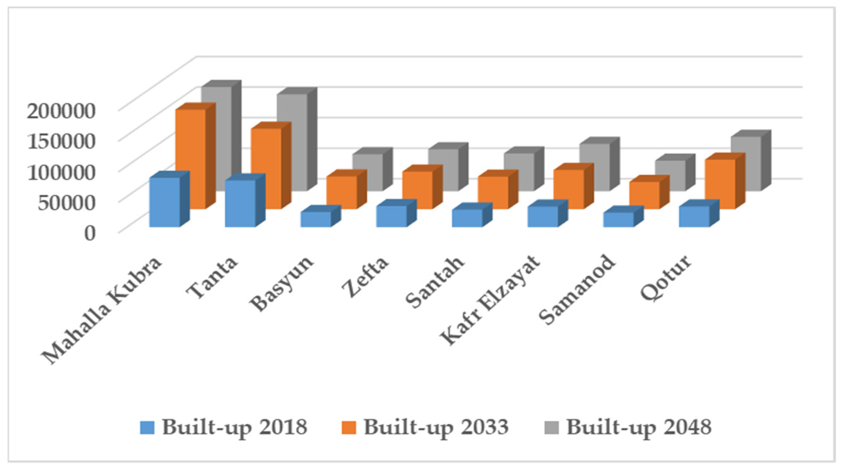
3.3. LULC Change Modeling, Simulation, and Projection

Before the prediction of the future LULC, the transition probability and transition area matrices were retrieved depending on the MC stochastic model using 1991 and 2003 LULC maps to simulate the 2018 LULC map (Figure 6a) for the model validation. These matrices and the transition probability maps have been inserted in the Supplementary Materials (Tables S4–S6 and Figures S1–S3 respectively). The model directly outputs the Kappa coefficient and the details have been inserted in the Supplementary Materials (Figure S4). Jaccard similarity coefficient were 88% and 52%, respectively. The Kappa coefficient directly output The Jaccard coefficient statistic better estimates the fit between the observed and simulated LULC maps. The results were considered adequately acceptable, and the model could be adopted for future simulation. The model was employed to extrapolate future LULC maps for 2033 and 2048, as clarified in Figure 6b,c, respectively.

For the future prediction step, the spatial modeling variables were updated from the first time period to the second time period before running the projection. Subsequently, the model predicted the potential changes in the following 30 years based on the 2018 LULC, assuming that there is no emergency, such as policy changes. The logistic regression algorithm was sufficient in the evaluation of the spatial relationships between the observed LULCC and predictor variables, generating the transition probability maps. According to our LULC predictions, the water bodies almost remain without changes. Therefore, this class is discarded. Thus, when we address the 2018–2048 period, we consider the change of built-up and agricultural land. It is predicted that built-up lands will cover 29% and 33% of the total land area by 2033 and 2048, respectively.

As clarified in

Table 7. Details of LULCC in Gharbia governorate in 2018 (simulated), 2033, and 2048.

LULC	2018		2033		2048		RD% 2018–2033	RD% 2018–2048
	Area (km2)	%	Area (km2)	%	Area (km2)	%
Built-up	279.48	14.0	588.24	29.4	663.68	33.2	+110.5	+137.5
Water	48.59	2.4	20.65	1.1	19.11	1.0	−57.5	−60.7
Agricultural land	1671.26	83.6	1390.44	69.5	1316.54	65.8	−16.8	−21.2
Total	1999.33	100	1999.33	100	1999.33	100

, the results showed that the trend of urban growth on the agricultural land is persistent. For instance, the built-up area will increase by about 14% (285 km²) and 18% (359 km²) by 2033 and 2048, respectively. In other words, the size of the urban cover will more than double through the 2018–2033 period. On the other hand, the agricultural land will decrease by the same percentage within the same study periods. The probable urban growth over the agricultural land (LULCC) within the time periods—2018–2033 and 2018–2048—is demonstrated in Figure 7a,b respectively. Moreover, as Figure 7 shows, the built-up area will be persistent around the centers of the governorate and the infrastructure, e.g., roads and railway stations.

Based on the results of the prediction, Figure 8 represents the size of the urban cover over the eight districts in 2018, 2033, and 2048. It reveals that Mahalla Kubra and Tanta are the districts suffering the most from urban growth dynamics, while Samanod suffers the least.

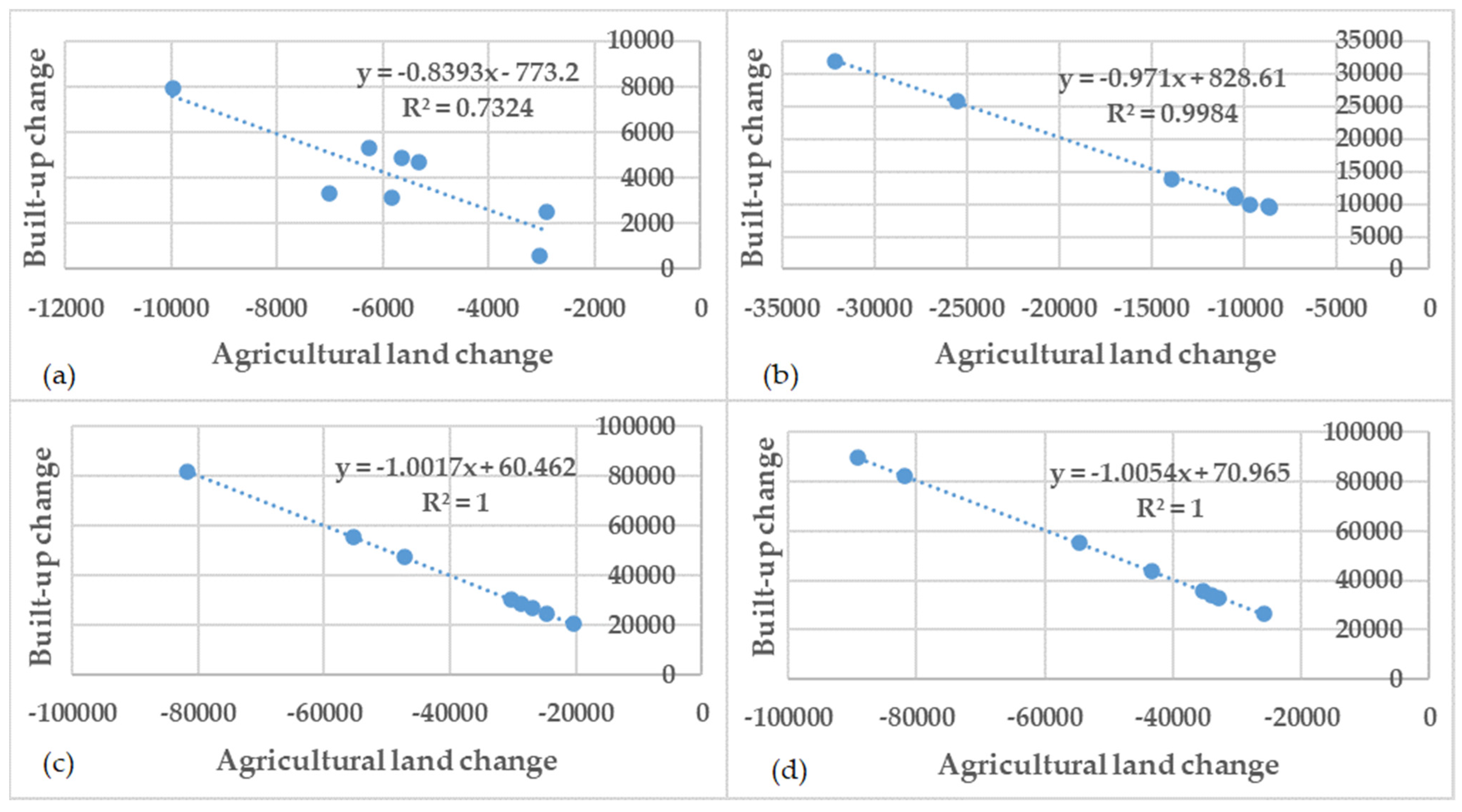
3.4. Linear Regression Analysis

A regression analysis was used to quantitatively estimate the relationship of the agricultural land change with the built-up area change [64] for the eight districts, as shown in Figure 9. The scatterplot illustrates the negative strong relationship, where the correlation coefficient (R²) equals 0.73 and 0.99 for the study periods of 1991–2003 and 2003–2018, respectively (Figure 9a,b). Furthermore, the predicted LULC demonstrates the same trend of correlation that the linear regression confirmed; the totally negative relationships where R² = 1 for the future study periods of 2018–2033 and 2018–2048 (Figure 9c,d).

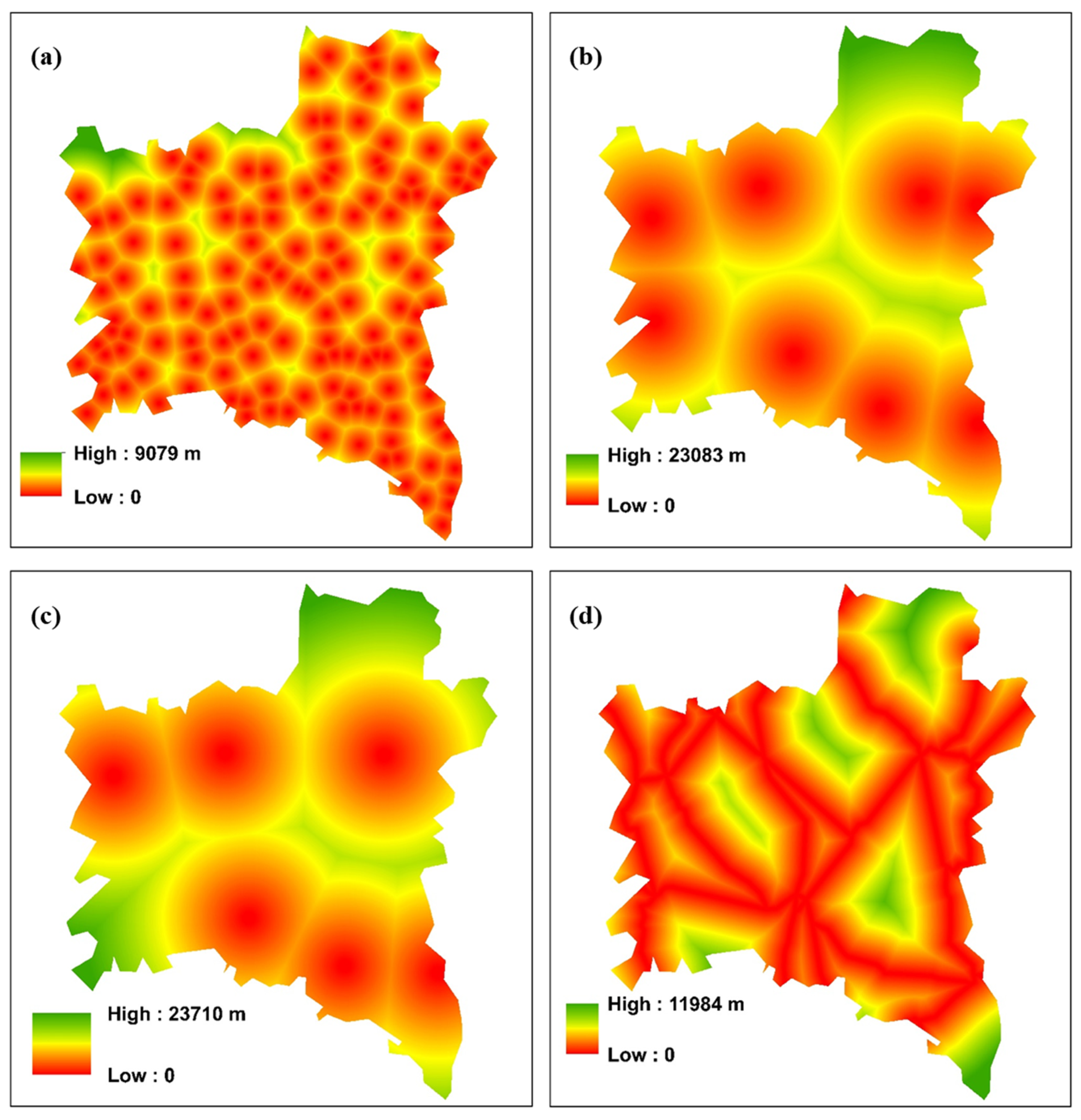
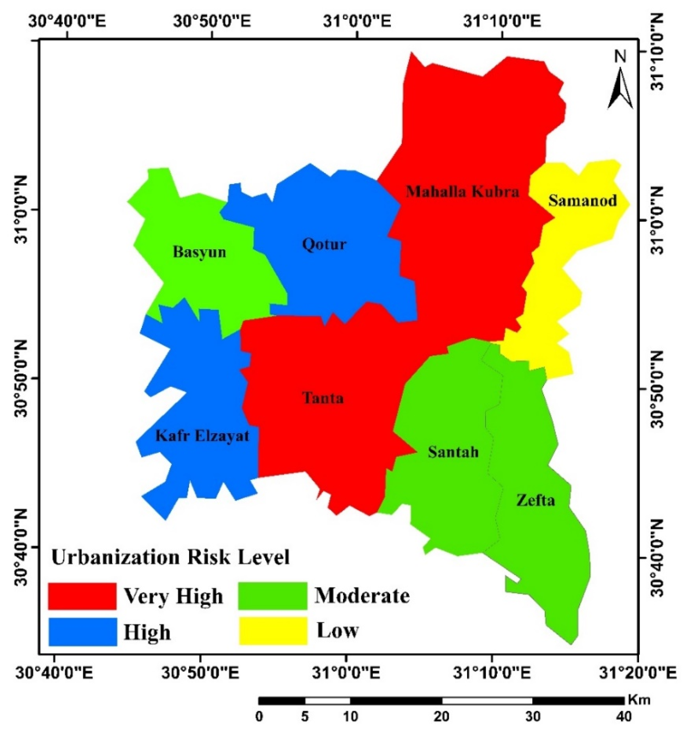
3.5. Analysis of Fuzzy TOPSIS

Based on the Fuzzy TOPSIS analysis and the criteria selected to evaluate the susceptibility of the districts to the urbanization risk, the closeness coefficient CCi, computed for each alternative, is shown in

Table 8. Closeness coefficient, CCi, for each alternative.

Criteria	CCi	Rank	Risk Level
Mahalla Kubra	1	1	V. High
Tanta	1	2	V. High
Basyun	0.055	7	Moderate
Zefta	0.19	5	Moderate
Santah	0.132	6	Moderate
Kafr Elzayat	0.577	3	High
Samanod	0.049	8	Low
Qotur	0.472	4	High

. The results showed that the Mahalla Kubra and Tanta districts are the most susceptible to the urbanization risk, while Samanod is the least susceptible. These results fit the results of the logistic regression–Markov prediction model. To clarify, the districts predicted to have bigger urban expansion are themselves certain to be highly susceptible to urbanization risk based on Fuzzy TOPSIS analysis.

It means that the results of the Fuzzy TOPSIS analysis can be adopted. On the other hand, if the area is not covered by the satellite images, Fuzzy TOPSIS can be employed to evaluate the districts’ susceptibility to the urbanization risk, in order for the decision-makers to be informed of the districts having the priority for sustainable planning, depending on the criteria analysis. Thus, producing the Urbanization Risk Map without satellite data is possible. Figure 10 shows a visual representation of the districts with their corresponding susceptibility level to urbanization risk. This confirms that Fuzzy TOPSIS analysis is superior for the production of an Urbanization Risk Map.

4. Discussion

Based on the quantification of the LULC changes throughout the study area over the study period (27 years), from 1991 to 2018, the agricultural land was dominant. However, rapid and ongoing urbanization has occurred. The mounting population necessitates the construction of facilities and the development of transportation systems to meet the increasing social and economic requirements. This is why policymakers and planners are particularly concerned with urbanization patterns, as they are crucial for effective decision-making.

The LULC maps for the years 1991, 2003, and 2018 emphasize a persistent trend of urban growth in the study area. The built-up land almost doubled, while the agricultural land exhibited an inverse pattern over the study period, where the urban expansion corresponded to loss of agricultural land. The decreasing trend of agricultural land was more significant during the second time period (2003–2018) compared to the first time period (1991–2003). This mentions that there is increased demand or pressure on land by the sprawling population due to increased rural–urban migration, and Gharbia governorate especially does not have a desert yard that permits urban expansion. Many previous studies have suffered from encroachment on arable and already-cultivated lands [13,34]. Therefore, the government seeks to deal with the crisis.

According to this study, the change in water bodies would be negligible. Therefore, the transition potential from agricultural land to built-up land, expressing the phenomenon of urban sprawl, was focused. We selected four spatial modeling variables as possible driving forces of LULCC, which have been specifically defined as urban sprawl parameters. In the model validation, the Kappa and Jaccard coefficients reached 88% and 52%, respectively. The Jaccard coefficient statistic was preferred to cross-check the results [71], as it considers how much correspondence—spatially and with quantitatively—there is between the two layers. In other words, it is a statistic which is used to gauge the similarity and diversity of sample sets. Therefore, the Jaccard coefficient is more realistic and reliable, as it considers the location of the LULCC, not only its quantity. The Jaccard value is affected by LULC classes, the annual rate of change, and transition steps [69]. The usually acceptable values are >60%. However, the model can be adopted for simulation and prediction. The urban sprawl on the agricultural land through the first period (1991–2003) was much lower than the urban growth experienced through the second time period (2003–2018) due to the lawlessness that happened in the country during the 2011 revolution. Therefore, the quantity of the actual urban area in 2018 was higher than the simulated one. Subsequently, the Jaccard coefficient of 52% in this study can be accepted, and the model can be used for further simulation and future projection. It is worthwhile to mention that if the acquired satellite images were chosen at close and equal intervals, and there is no sudden boom in a certain period (as in our case), the logistic regression–Markov model would give more satisfying results, and the validated outputs would match the actual land-use image spatially and quantitatively.

We adopted the logistic regression owing to its demonstrated accuracy when modeling LULC transitions, and the unique advantage of its unneeded prior knowledge compared to other different models. The previous studies’ results showed that the logistic regression model was qualified for the production of realistic results in the respective study areas [33,34,35]. For instance, Hamdy et al. [34] applied a hybrid approach of the Markov chain and logistic regression models to define future urban spread in 2037 in Abouelreesh, Aswan, Egypt. The consequences of their paper highlight the growing risks of urban expansion and the obstacles which object to the sustainable urban growth strategies recommended for this area. Furthermore, Arsanjani et al. [33] adopted a hybrid model including logistic regression, MC, and CA, which was prepared to upgrade the performance of the basic logistic regression model. The simulated map fitted the actual one by 89%, which was satisfactory for the adoption of the calibration process. The simulated maps show a fresh wave of suburban evolution in the proximity of Tehran over the coming decades. Nguyen et al. [35] also used the same hybrid model of the logistic regression, MC, and CA models for the prediction of the future land-use change in Nam Dinh Province, Vietnam. The hybrid model was sufficient, and the outcomes of the analysis present worthy knowledge for local planners and policymakers, supporting their efforts in organizing other sustainable urban planning schemas and environmental management policies. Therefore, this approach could be adopted for the identification of patterns of LULC changes in the Gharbia governorate.

The predicted maps show that the same trend of agricultural land loss due to urban growth can be expected for 2033 and 2048. A similar pattern of agricultural land diminution could be evident in the preceding studies. Our study did not only focus on monitoring and forecasting the urban expansion like all of the previous studies; it also adopted Fuzzy TOPSIS analysis based on criteria selected to evaluate the susceptibility of the districts to the urbanization risk, which is effective for the data-gap regions. In other words, if the satellite data are scarce for the area of interest, Fuzzy TOPSIS can evaluate the districts’ susceptibility to the urbanization risk, in order for the decision-makers to be informed of the districts with the priority for sustainable planning. Thus, producing the Urbanization Risk Map without satellite data is possible. Otherwise, if the area of interest is covered by satellite images, our methodology outperforms other methodologies due to the further validation performed for the prediction results from the logistic regression–Markov model based on Fuzzy TOPSIS; the predicted size of the urban extent in a district corresponds to the level of urbanization risk for that district.

According to our prediction results, if the current condition of urban sprawl continues at the pace of 2018, about 285 km² of agricultural land will change into built-up land by 2033, and a further 73 km² by 2048, which could cause a considerable change to the social and economic conditions in the area. The built-up lands will cover 29% and 33% of the total land area by 2033 and 2048, respectively. This is a negative indication of the loss of agricultural land, hence the food security issue, especially with the population growing in a random way that is not proportional to the land area and the loss of agricultural land. If the government does not address urban encroachment on agricultural land, built-up land will represent more than a quarter of the total area by 2033, and a third by 2048. This rate of urban sprawl is a cause for concern.

The continuous and rapid urbanization over the cultivated land has serious consequences for agricultural productivity and the sustainability of the country’s economic development [14]. The Egyptian government has lately initiated a number of projects to reclaim new desert lands to meet the rising demand for food due to the country’s rapid population increase. These attempts can be regarded as a possible solution to the existing issue. However, it is not the best solution, as we mentioned before that the newly reclaimed lands do not compensate for the corresponding deduction of the old ones, because the soil is less fertile and has much lower nutrient levels than the old soil [2]. Moreover, the reclaimed desert land costs a lot to provide the required resources like power, water, and chemical fertilizers to increase the soil fertility, as well as the required labor and safe transportation to remote markets [2,38]. This means creates a need for considerable funding to upgrade the soil fertility. Therefore, most newly reclaimed desert lands are planted with products for export to achieve a profit that compensates for the cost of reclamation, and thus this policy does not participate in solving the problem of food and self-sufficiency for the country [2]. Accordingly, the government has to adopt other strategies to address massive population growth and rapid urbanization. For instance, as suggestions, (1) urbanization could expand vertically in the defined urban area, in addition to conservation of existing fertile soil areas and the maximization of the agricultural productivity of existing cultivated areas; (2) structure sustainable cities outside the borders of the delta, to accommodate the population increase, associated with the required infrastructure for a convenient life. The reconstruction of the desert is the best proposal to relieve the pressure on the delta region, and to stop more urban expansion inside this green zone of the Nile Delta. Accordingly, the expected changes in LULC may provide the proper planning for the practical and sustainable use of resources.

There are three prime sources of uncertainty in machine learning: noise in the data, the incomplete coverage of the domain, and imperfect models [80]. All of the measurements have an amount of uncertainty regardless of the precision and accuracy. Uncertainty is a common phenomenon in many application areas, such as medicine, image processing, and linguistics, etc. [81]. For example (for medicine), frequently, medical diagnosis is not improper, but there are different degrees of disease. Consequently, uncertainty occurs almost automatically in any machine learning application [81]. Therefore, we recommend further research to consider the uncertainty in machine learning methods, particularly in critical domains such as clinical diagnosis, and in safety-critical areas which need output decisions accompanied by a measure that allows the judgement of the certainty of the output.

In addition, another limitation in this study, which is considered as the most evident limitation in machine learning, is the data [82]. Several machine learning algorithms need considerable quantities of data before they can start giving beneficial results [83,84]. A good illustration of this is the neural network. Neural networks are data-consuming machines that demand extensive volumes of training data. Algorithms trained on insufficient datasets have uncertain performance when applied to further unseen data sets [85], and therefore the model will overfit. The overfitting model works very well on the data used to train it but works poorly on new data (test data) [86,87]. So, it’s the user’s responsibility to regulate the learning process. There are diverse methods to avoid overfitting [88], e.g., (1) training with more data [89], the model will not be capable of overfitting all of the samples and will have to generalize to get the results; (2) data augmentation [90], which makes sample data look rather various each time it is processed by the model. This prevents the model from learning the properties of the datasets; and (3) the data simplification method [86] is utilized to minimize overfitting by reducing the complexity of the model in order to make it adequately simple, such that it does not overfit. The performance of an algorithm relies not only on the data quantity but also on the data quality; hence, algorithms are as good as the data they are trained on [85]. Training algorithms the same way we learn ourselves comes with limitations. Unfortunately, the usage of unrepresentative or insufficient data has an adverse influence on performance. In the same way that a lack of good features can lead to poor algorithm performance, a lack of good ground truth data can also reduce the potential of the model [91]. Accordingly, we recommend depending on algorithms which need less data for training, like SVM, or providing the required data and taking into account the uncertainty.

5. Conclusions

This study focused on persistent urban growth at the expense of agricultural land in the eight districts of Gharbia governorate. This will cause gross problems later if the current land-use policy is ongoing. Therefore, the government has to find an alternative trend of land-use, e.g., desert development, to stop more urban expansion inside the green zone of the Nile Delta. This is frequently successful in preserving fertile cultivated lands.

In this study, the LULC dynamics in the Gharbia governorate were monitored and assessed over a 27-year study period from 1991 to 2018, and the future trends to 2033 and 2048 were investigated using a hybrid model of MC and logistic regression. Markov chain–logistic regression was sufficient in the modeling of the LULC transitions, where the MC model is very superior in quantifying the transitions and detecting the conversion rates between various LULC types, and logistic regression is capable of providing transition potential maps. There was a trend of rapid urbanization over the agricultural land. In the prediction of the future dynamics of LULC the same trend continues, indicating negative aspects such as the issue of food security. The agricultural land is declining at a worrisome rate; it occupied 91.2% of the total land area in 1991, and will decline to 65.8% in 2048. This persistent urbanization will affect the climate of the region (increasing the temperature and affecting residents’ life) and cause the imbalance of ecosystem services. Furthermore, the loss of agricultural land may put the agricultural activity of the governorate at risk. Therefore, the government has to change policy and address such problems, especially in the areas without desert backyards.

Defining the pattern of LULC changes (in terms of quantity and direction) is substantial for the decision-makers and planners for sustainable urban planning and the confrontation of the challenges created by rapid unplanned urban growth. The innovation of this work is as follows: (1) this article presents machine learning-based and state-of-the-art remote sensing-based products and methodologies for the continuous monitoring of LULC for sustainable land-use policies, and (2) the current paper highlights the vital role of the Fuzzy TOPSIS method, which eliminates uncertainties in the data and analysis for the production of the Urbanization Risk Map, in order to determine the susceptibility of the districts to the urbanization risk, especially in the case of unavailable satellite images, in order for the decision-maker to be given the districts with the priority for sustainable land-use planning.

The medium spatial resolution of Landsat images is considered a shortcoming. Usually, the free data have a lower spatial resolution which cannot allow the perfect quantification of the LULC dynamics, especially given that the LULCC affects the climate. Therefore, an archive of images is in demand. However, SVM is superior in the classification process. Furthermore, uncertainty is a common phenomenon in machine learning. All of the measurements have an amount of uncertainty regardless of their precision and accuracy. Therefore, we recommend further research to consider the uncertainty in machine learning methods, particularly in critical domains such as clinical diagnosis. We suggest that future studies persist with new data and models to evolve the simulations that address uncertainties in future LULC.

References

1. Seto, K.C.; Güneralp, B.; Hutyra, L.R. Global forecasts of urban expansion to 2030 and direct impacts on biodiversity and carbon pools. Proc. Natl. Acad. Sci. USA 2012, 109, 16083–16088. [Google Scholar] [CrossRef] [PubMed] [Green Version]
2. Bakr, N.; Bahnassy, M.H. Egyptian Natural Resources. In The Soils of Egypt, 1st ed.; El-Ramady, H., Alshaal, T., Bakr, N., Elbana, T., Mohamed, E., Belal, A.A., Eds.; Springer: Cham, Switzerland, 2019; pp. 33–49. [Google Scholar]
3. Van Vliet, J.; Eitelberg, D.A.; Verburg, P.H. A global analysis of land take in cropland areas and production displacement from urbanization. Glob. Environ. Chang. 2017, 43, 107–115. [Google Scholar] [CrossRef]
4. Zhao, S.; Da, L.; Tang, Z.; Fang, H.; Song, K.; Fang, J. Ecological consequences of rapid urban expansion: Shanghai, China. Front. Ecol. Environ. 2006, 4, 341–346. [Google Scholar] [CrossRef]
5. Grimm, N.B.; Faeth, S.H.; Golubiewski, N.E.; Redman, C.L.; Wu, J.; Bai, X.; Briggs, J.M. Global change and the ecology of cities. Science 2008, 319, 756–760. [Google Scholar] [CrossRef] [PubMed] [Green Version]
6. Linard, C.; Tatem, A.J.; Gilbert, M. Modelling spatial patterns of urban growth in africa. Appl. Geogr. 2013, 44, 23–32. [Google Scholar] [CrossRef]
7. Wu, Y.; Li, S.; Yu, S. Monitoring urban expansion and its effects on land use and land cover changes in Guangzhou city, China. Environ. Monit. Assess. 2016, 188, 1–15. [Google Scholar] [CrossRef]
8. Guan, D.; Li, H.; Inohae, T.; Su, W.; Nagaie, T.; Hokao, K. Modeling urban land use change by the integration of cellular automaton and Markov model. Ecol. Model. 2011, 222, 3761–3772. [Google Scholar] [CrossRef]
9. Ranagalage, M.; Wang, R.; Gunarathna, M.H.J.P.; Dissanayake, D.M.S.L.B.; Murayama, Y.; Simwanda, M. Spatial forecasting of the landscape in rapidly urbanizing hill stations of South Asia: A case study of Nuwara Eliya, Sri Lanka (1996–2037). Remote Sens. 2019, 11, 1743. [Google Scholar] [CrossRef] [Green Version]
10. Rimal, B.; Sloan, S.; Keshtkar, H.; Sharma, R.; Rijal, S.; Shrestha, U.B. Patterns of historical and future urban expansion in Nepal. Remote Sens. 2020, 12, 628. [Google Scholar] [CrossRef] [Green Version]
11. Dewan, A.M.; Corner, R.J. Spatiotemporal analysis of urban growth, sprawl and structure. In Dhaka Megacity, Geospatial Perspectives on Urbanization, Environment and Health; Springer: New York, NY, USA, 2013. [Google Scholar]
12. El-Eraqi, M.B.; Shehata, M.S. The Urban Sprawl on Agricultural Lands in Gharbia Govornorate. Ar. Univ. J. Agric. Sci. 2019, 27, 1771–1781. [Google Scholar]
13. Radwan, T.M.; Blackburn, G.A.; Whyatt, J.D.; Atkinson, P.M. Dramatic loss of agricultural land due to urban expansion threatens food security in the Nile Delta, Egypt. Remote Sens. 2019, 11, 332. [Google Scholar] [CrossRef] [Green Version]
14. Abd El-Kawy, O.R.; Rød, J.K.; Ismail, H.A.; Suliman, A.S. Land use and land cover change detection in the western Nile delta of Egypt using remote sensing data. Appl. Geogr. 2011, 31, 483–494. [Google Scholar] [CrossRef]
15. Bratley, K.; Ghoneim, E. Modeling Urban Encroachment on the Agricultural Land of the Eastern Nile Delta Using Remote Sensing and a GIS-Based Markov Chain Model. Land 2018, 7, 114. [Google Scholar] [CrossRef] [Green Version]
16. Bakr, N.; Weindorf, D.C.; Bahnassy, M.H.; Marei, S.M.; El-Badawi, M.M. Monitoring land cover changes in a newly reclaimed area of Egypt using multi-temporal Landsat data. Appl. Geogr. 2010, 30, 592–605. [Google Scholar] [CrossRef]
17. Sarker, I.H.; Hoque, M.M.; Uddin, M.K.; Alsanoosy, T. Mobile data science and intelligent apps: Concepts, ai-based modeling and research directions. Mob. Netw. Appl. 2021, 26, 285–303. [Google Scholar] [CrossRef]
18. Rai, R.; Zhang, Y.; Paudel, B.; Acharya, B.; Basnet, L. Land use and land cover dynamics and assessing the ecosystem service values in the trans-boundary gandaki river basin, central himalayas. Sustainability 2018, 10, 3052. [Google Scholar] [CrossRef] [Green Version]
19. Liping, C.; Yujun, S.; Saeed, S. Monitoring and predicting land use and land cover changes using remote sensing and gis techniques—A case study of a hilly area, Jiangle, China. PLoS ONE 2018, 13, e0200493. [Google Scholar] [CrossRef] [PubMed]
20. Sarker, I.H.; Kayes, A.S.M.; Badsha, S.; Alqahtani, H.; Watters, P.; Ng, A. Cybersecurity data science: An overview from machine learning perspective. J. Big Data 2020, 7, 1–29. [Google Scholar] [CrossRef]
21. Han, J.; Pei, J.; Kamber, M. Data Mining: Concepts and Techniques; Elsevier: Amsterdam, The Netherlands, 2011. [Google Scholar]
22. Bray, M.; Han, D. Identification of support vector machines for runoff modelling. J. Hydroinform. 2004, 6, 265–280. [Google Scholar] [CrossRef] [Green Version]
23. Cortes, C.; Vapnik, V. Support-vector networks. Mach. Learning 1995, 20, 273–297. [Google Scholar] [CrossRef]
24. Moghaddamnia, A.; Gosheh, M.; Nuraie, M.; Mansuri, M.; Han, D.; Schmitter, E. Performance evaluation of LLR, SVM, CGNN and BFGSNN models to evaporation estimation. Water Geosci. 2010, 9, 108–113. [Google Scholar]
25. Han, D.; Chan, L.; Zhu, N. Flood forecasting using support vector machines. J. Hydroinform. 2007, 9, 267–276. [Google Scholar] [CrossRef]
26. Taati, A.; Sarmadian, F.; Mousavi, A.; Pour, C.T.H.; Shahir, A.H.E. Land use classification using support vector machine and maximum likelihood algorithms by Landsat 5 TM images. Walailak J. Sci. Tech. (WJST) 2015, 12, 681–687. [Google Scholar]
27. Yousefi, S.; Tazeh, M.; Mirzaee, S.; Moradi, H.R.; Tavangar, S.H. Comparison of different classification algorithms in satellite imagery to produce land use maps (Case study: Noor city). J. Appl. RS GIS Tech. Nat. Res. Sci. 2011, 2, 15–25. [Google Scholar]
28. Clarke, K.C. Land use change modeling with sleuth: Improving calibration with a genetic algorithm. In Geomatic Approaches for Modeling Land Change Scenarios; Camacho Olmedo, M.T., Paegelow, M., Mas, J.-F., Escobar, F., Eds.; Springer International Publishing: Cham, Switzerland, 2018; pp. 139–161. [Google Scholar]
29. Verburg, P.H.; Overmars, K.P. Dynamic simulation of land-use change trajectories with the clue-s model. In Modelling Land-Use Change: Progress and Applications; Koomen, E., Stillwell, J., Bakema, A., Scholten, H.J., Eds.; Springer: Dordrecht, The Netherlands, 2007; pp. 321–337. [Google Scholar]
30. Kuo, H.-F.; Tsou, K.-W. Modeling and simulation of the future impacts of urban land use change on the natural environment by sleuth and cluster analysis. Sustainability 2018, 10, 72. [Google Scholar] [CrossRef] [Green Version]
31. Chen, C.; Son, N.; Chang, N.; Chen, C.; Chang, L.; Valdez, M.; Centeno, G.; Thompson, C.A.; Aceituno, J.L. Multi-decadal mangrove forest change detection and prediction in Honduras, Central America, with Landsat imagery and a Markov Chain Model. Remote Sens. 2013, 5, 6408–6426. [Google Scholar] [CrossRef] [Green Version]
32. Weiguo, J.; Zheng, C.; Xuan, L.E.I.; Kai, J.I.A.; Yongfeng, W.U. Simulating urban land use change by incorporating an autologistic regression model into a CLUE-S model. J. Geogr. Sci. 2015, 25, 836–850. [Google Scholar]
33. Arsanjani, J.J.; Helbich, M.; Kainz, W.; Boloorani, A.D. Integration of logistic regression, markov chain and cellular automata models to simulate urban expansion. Int. J. Appl. Earth Obs. Geoinf. 2013, 21, 265–275. [Google Scholar] [CrossRef]
34. Hamdy, O.; Zhao, S.; Osman, T.; Salheen, M.A.; Eid, Y.Y. Applying a hybrid model of Markov chain and logistic regression to identify future urban sprawl in Abouelreesh, Aswan: A case study. Geosciences 2016, 6, 43. [Google Scholar] [CrossRef] [Green Version]
35. Nguyen, V.T.; Le, T.T.H.; La, P.H. Predicting land use change affected by population growth by integrating logistic regression, Markov chain and cellular automata models. J. Korean Soc. Surv. Geod. Photogramm Cart. 2017, 35, 221–230. [Google Scholar]
36. Verhagen, P. Case Studies in Archaeological Predictive Modeling; Amsterdam University Press: Amsterdam, The Netherlands, 2007. [Google Scholar]
37. Dewan, A.M.; Yamaguchi, Y. Land use and land cover change in Greater Dhaka, Bangladesh: Using remote sensing to promote sustainable urbanization. Appl. Geogr. 2009, 29, 390–401. [Google Scholar] [CrossRef]
38. Negm, A.M.; Saavedra, O.; El-Adawy, A. Nile Delta Biography: Challenges and Opportunities. In The Nile Delta; Negm, A., Ed.; The Handbook of Environmental Chemistry; Springer: Cham, Switzerland, 2016; Volume 55. [Google Scholar]
39. Erkan, U.; Gökrem, L. A new method based on pixel density in salt and pepper noise removal. Turk. J. Electr. Eng. Comput. Sci. 2018, 26, 162–171. [Google Scholar] [CrossRef]
40. Sakthidasan, K.; Nagappan, N.V. Noise free image restoration using hybrid filter with adaptive genetic algorithm. Comput. Electr. Eng. 2016, 54, 382–392. [Google Scholar] [CrossRef]
41. Vivekananda, G.N.; Swathi, R.; Sujith, A.V.L.N. Multi-temporal image analysis for LULC classification and change detection. Eur. J. Remote. Sens. 2021, 54 (Suppl. S2), 189–199. [Google Scholar] [CrossRef]
42. Talukdar, S.; Singha, P.; Mahato, S.; Pal, S.; Liou, Y.A.; Rahman, A. Land-use land-cover classification by machine learning classifiers for satellite observations—A review. Remote Sens. 2020, 12, 1135. [Google Scholar] [CrossRef] [Green Version]
43. Foody, G.M. Status of land cover classification accuracy assessment. Remote Sens. Environ. 2002, 80, 185–201. [Google Scholar] [CrossRef]
44. Bharatkar, P.S.; Patel, R. Approach to accuracy assessment tor RS image classification techniques. Int. J. Sci. Eng. Res. 2013, 4, 79–86. [Google Scholar]
45. Li, C. Monitoring and Analysis of Urban Growth Process Using Remote Sensing, GIS and Cellular Automata Modeling: A Case Study of Xuzhou City, China. Ph.D. Thesis, Universitätsbibliothek, Dortmund, Germany, September 2014. [Google Scholar]
46. Ramachandra, T.V.; Aithal, H.B.; Vinay, S.; Joshi, N.V.; Kumar, U.; Rao, K.V. Modelling urban revolution in Greater Bangalore, India. In Proceedings of the 30th Annual In-House Symposium on Space Science and Technology, Bangalore, India, 7–8 November 2013; pp. 7–8. [Google Scholar]
47. Sang, L.; Zhang, C.; Yang, J.; Zhu, D.; Yun, W. Simulation of land use spatial pattern of towns and villages based on CA-Markov model. Math. Comput. Model. 2011, 54, 938–943. [Google Scholar] [CrossRef]
48. Kore, N.B.; Ravi, K.; Patil, S.B. A simplified description of fuzzy TOPSIS method for multi criteria decision making. Int. Res. J. Eng. Tech. (IRJET) 2017, 4, 2047–2050. [Google Scholar]
49. Gutiérrez, S.; Tardaguila, J.; Fernández-Novales, J.; Diago, M.P. Support vector machine and artificial neural network models for the classification of grapevine varieties using a portable NIR spectrophotometer. PLoS ONE 2015, 10, e0143197. [Google Scholar] [CrossRef]
50. Mustafa, E.K.; Co, Y.; Liu, G.; Kaloop, M.R.; Beshr, A.A.; Zarzoura, F.; Sadek, M. Study for Predicting Land Surface Temperature (LST) Using Landsat Data: A Comparison of Four Algorithms. Adv. Civ. Eng. 2020, 2020, 7363546. [Google Scholar] [CrossRef]
51. Sadek, M.; Li, X. Low-cost solution for assessment of urban flash flood impacts using sentinel-2 satellite images and fuzzy analytic hierarchy process: A case study of ras ghareb city, Egypt. Adv. Civ. Eng. 2019, 2019, 2561215. [Google Scholar] [CrossRef] [Green Version]
52. Almouctar, M.A.S.; Wu, Y.; Kumar, A.; Zhao, F.; Mambu, K.J.; Sadek, M. Spatiotemporal analysis of vegetation cover changes around surface water based on NDVI: A case study in Korama basin, Southern Zinder, Niger. Appl. Water Sci. 2020, 11, 1–14. [Google Scholar] [CrossRef]
53. Kamusoko, C.; Aniya, M. Hybrid classification of Landsat data and GIS for land use/cover change analysis of the Bindura district, Zimbabwe. Int. J. Remote Sens. 2008, 30, 97–115. [Google Scholar] [CrossRef]
54. Sadek, M.; Li, X.; Mostafa, E.; Freeshah, M.; Kamal, A.; Sidi Almouctar, M.A.; Mustafa, E.K. Low-Cost Solutions for Assessment of Flash Flood Impacts Using Sentinel-1/2 Data Fusion and Hydrologic/Hydraulic Modeling: Wadi El-Natrun Region, Egypt. Adv. Civ. Eng. 2020. [Google Scholar] [CrossRef]
55. Dossou, J.; Li, X.; Sadek, M.; Mostafa, E. Hybrid model of ecological vulnerability assessment in Benin. Sci. Rep. 2021. Available online: https://www.nature.com/articles/s41598-021-81742-2 (accessed on 21 June 2021). [CrossRef]
56. Rousta, I.; Sarif, M.O.; Gupta, R.D.; Olafsson, H.; Ranagalage, M.; Murayama, Y.; Zhang, H.; Mushore, T.D. Spatiotemporal analysis of land use/land cover and its effects on surface urban heat island using Landsat data: A case study of metropolitan city Tehran (1988–2018). Sustainability 2018, 10, 4433. [Google Scholar] [CrossRef] [Green Version]
57. Dissanayake, D.; Morimoto, T.; Murayama, Y.; Ranagalage, M. Impact of landscape structure on the variation of land surface temperature in sub-saharan region: A case study of Addis Ababa using Landsat data (1986–2016). Sustainability 2019, 11, 2257. [Google Scholar] [CrossRef] [Green Version]
58. Hamdy, O.; Zhao, S.; Salheen, M.A.; Eid, Y.Y. Analyses the driving forces for urban growth by using IDRISI® Selva Models Abouelreesh Aswan as a Case Study. Int. J. Eng. Technol. 2017, 9, 226. [Google Scholar] [CrossRef] [Green Version]
59. Eastman, J.R. Manual for Using Terrset; Clark Labs, Clark University: Worcester, MA, USA, 2018. [Google Scholar]
60. CLARK LAB. Available online: https://clarklabs.org (accessed on 8 September 2019).
61. Rizk, I.; Rashed, M. Monitoring urban growth and land use change detection with GIS and remote sensing techniques in Daqahlia governorate Egypt. Int. J. Sustain. Built Environ. 2015, 4, 117–124. [Google Scholar]
62. Rimal, B.; Zhang, L.; Keshtkar, H.; Wang, N.; Lin, Y. Monitoring and modeling of spatiotemporal urban expansion and land-use/land-cover change using integrated Markov chain cellular automata model. ISPRS Int. J. Geo-Inf. 2017, 6, 288. [Google Scholar] [CrossRef] [Green Version]
63. Keshtkar, H.; Voigt, W. Potential impacts of climate and landscape fragmentation changes on plant distributions: Coupling multi-temporal satellite imagery with gis-based cellular automata model. Ecol. Inform. 2016, 32, 145–155. [Google Scholar] [CrossRef]
64. Hou, H.; Wang, R.; Murayama, Y. Scenario-based modelling for urban sustainability focusing on changes in cropland under rapid urbanization: A case study of Hangzhou from 1990 to 2035. Sci. Total Environ. 2019, 661, 422–431. [Google Scholar] [CrossRef]
65. Wang, R.; Derdouri, A.; Murayama, Y. Spatiotemporal simulation of future land use/cover change scenarios in the Tokyo metropolitan area. Sustainability 2018, 10, 2056. [Google Scholar] [CrossRef] [Green Version]
66. Subasinghe, S.; Estoque, R.C.; Murayama, Y. Spatiotemporal analysis of urban growth using GIS and remote sensing: A case study of the Colombo Metropolitan Area, Sri Lanka. ISPRS Int. J. Geo-Inf. 2016, 5, 197. [Google Scholar] [CrossRef] [Green Version]
67. Thapa, R.B.; Murayama, Y. Scenario based urban growth allocation in Kathmandu Valley, Nepal. Landsc. Urban Plan. 2012, 105, 140–148. [Google Scholar] [CrossRef]
68. Mishra, V.N.; Rai, P.K. A remote sensing aided multi-layer perceptron-Markov chain analysis for land use and land cover change prediction in Patna district (Bihar), India. Arab. J. Geosci. 2016, 9, 249. [Google Scholar] [CrossRef]
69. Estoque, R.C.; Murayama, Y. Examining the potential impact of land use/cover changes on the ecosystem services of Baguio city, the Philippines: A scenario-based analysis. Appl. Geogr. 2012, 35, 316–326. [Google Scholar] [CrossRef]
70. Ahmed, B.; Ahmed, R.; Zhu, X. Evaluation of model validation techniques in land cover dynamics. ISPRS Int. J. Geo-Inf. 2013, 2, 577–597. [Google Scholar] [CrossRef]
71. Van Vliet, J.; Bregt, A.K.; Hagen-zanker, A. Revisiting Kappa to account for change in the accuracy assessment of land-use change models. Ecol. Model. 2011, 222, 1367–1375. [Google Scholar] [CrossRef]
72. Landis, J.R.; Koch, G.G. The measurement of observer agreement for categorical Data. Biometrics 1977, 33, 159–174. [Google Scholar] [CrossRef] [PubMed] [Green Version]
73. Flo, J.; Landmark, B.; Hatlevik, O.E.; Fagerström, L. Using a new interrater reliability method to test the modified oulu patient classification instrument in home health care. Nurs. Open 2018, 5, 167–175. [Google Scholar] [CrossRef] [Green Version]
74. Pontius, R.G., Jr.; Millones, M. Death to Kappa: Birth of quantity disagreement and allocation disagreement for accuracy assessment. Int. J. Remote Sens. 2011, 32, 4407–4429. [Google Scholar] [CrossRef]
75. Sadek, M.; Li, X.; Mostafa, E.; Dossou, J. Monitoring Flash Flood Hazard Using Modeling-Based Techniques and Multi-Source Remotely Sensed Data in Ras Ghareb City, Egypt. Arab. J. Geosci. 2021, 14, 1–16. [Google Scholar] [CrossRef]
76. Ghar, M.A.; Shalaby, A.; Tateishi, R. Agricultural land monitoring in the Egyptian Nile Delta using landsat data. Int. J. Environ. Stud. 2004, 61, 651–657. [Google Scholar] [CrossRef]
77. Hwang, C.L.; Yoon, K.P. Multiple Attribute Decision Making: Methods and Applications, A State-of-the-Art Survey; Springer-Verlang: Berlin, Germany, 1981. [Google Scholar]
78. Chen, C.T. Extension of the TOPSIS for group decision-making under fuzzy environment. Fuzzy Sets Syst. 2000, 114, 1–9. [Google Scholar] [CrossRef]
79. Nădăban, S.; Dzitac, S.; Dzitac, I. Fuzzy TOPSIS: A general view. Procedia Comput. Sci. 2016, 91, 823–831. [Google Scholar] [CrossRef] [Green Version]
80. Brownlee, J. Probability for Machine Learning: Discover How to Harness Uncertainty with Python. Machine Learning Mastery. 2019. Available online: https://machinelearningmastery.com/uncertainty-in-machine-learning/ (accessed on 29 September 2021).
81. Hammer, B.; Villmann, T. How to process uncertainty in machine learning? In Proceedings of the ESANN’2007—European Symposium on Artificial Neural Networks, Bruges, Belgium, 25–27 April 2007; pp. 79–90. [Google Scholar]
82. Towards Data Science, The Limitations of Machine Learning. Available online: https://towardsdatascience.com/the-limitations-of-machine-learning-a00e0c3040c6 (accessed on 29 September 2021).
83. Zhu, X.; Vondrick, C.; Fowlkes, C.C.; Ramanan, D. Do we need more training data? Int. J. Comput. Vis. 2016, 119, 76–92. [Google Scholar] [CrossRef] [Green Version]
84. LeCun, Y.; Bengio, Y.; Hinton, G. Deep learning. Nature 2015, 521, 436–444. [Google Scholar] [CrossRef]
85. Mastorakis, G. Human-like machine learning: Limitations and suggestions. arXiv 2018, arXiv:1811.06052. [Google Scholar]
86. Ying, X. An overview of overfitting and its solutions. J. Phys. Conf. Ser. 2019, 1168, 02202. [Google Scholar] [CrossRef]
87. Cawley, G.C.; Talbot, N.L. On over-fitting in model selection and subsequent selection bias in performance evaluation. J. Mach. Learn. Res. 2010, 11, 2079–2107. [Google Scholar]
88. Lever, J.; Krzywinski, M.; Altman, N. Points of significance: Model selection and overfitting. Nat. Methods 2016, 13, 703–705. [Google Scholar] [CrossRef]
89. CFI. Available online: https://corporatefinanceinstitute.com/resources/knowledge/other/overfitting/ (accessed on 29 October 2021).
90. Towards Data Science. Available online: https://towardsdatascience.com/8-simple-techniques-to-prevent-overfitting-4d443da2ef7d (accessed on 29 October 2021).
91. Li, S.; Song, W.; Fang, L.; Chen, Y.; Ghamisi, P.; Benediktsson, J.A. Deep learning for hyperspectral image classification: An overview. IEEE Trans. Geosci. Remote Sens. 2019, 57, 6690–6709. [Google Scholar] [CrossRef] [Green Version]
Figure 1. The study area of Gharbia Governorate, Egypt.
Remotesensing 13 04498 g001
Figure 2. The conceptual flowchart of the applied methodology.
Remotesensing 13 04498 g002
Figure 3. The four selected modeling variables: (a) the distance from persistent built-up area during 1991–2003; (b) the distance from urban centers; (c) the distance from railway stations; and (d) the distance from the nearest road.
Remotesensing 13 04498 g003
Figure 4. Spatial distribution of the LULC over the study area during the study period: (a) LULC in 1991, (b) LULC in 2003, (c) LULC in 2018.
Remotesensing 13 04498 g004
Figure 5. Gain of built-up area at the expense of agricultural land through the two study periods: (a) the period of 1991–2003, and (b) the period of 2003–2018.
Remotesensing 13 04498 g005
Figure 6. (a) Simulated LULC of 2018, and (b,c) the projected land cover for 2033 and 2048, respectively.
Remotesensing 13 04498 g006
Figure 7. Predicted Gain of the built-up area at the expense of agricultural land in (a) the period of 2018–2033, and (b) the period of 2018–2048.
Remotesensing 13 04498 g007
Figure 8. The size of the urbanization over the eight districts in 2018, 2033, and 2048.
Remotesensing 13 04498 g008
Figure 9. Regression Analysis of the agricultural land change versus the built-up change over the Gharbia districts during the last and future periods: (a) 1991–2003, (b) 2003–2018, (c) 2018–2033, and (d) 2018–2048.
Remotesensing 13 04498 g009
Figure 10. The Urbanization Risk Map.
Remotesensing 13 04498 g010