Article

Assessing Grapevine Nutrient Status from Unmanned Aerial System (UAS) Hyperspectral Imagery

1
Chester F. Carlson Center for Imaging Science, Rochester Institute of Technology, Rochester, NY 14623, USA
2
Horticulture Section, School of Integrative Plant Science, Cornell University, Ithaca, NY 14853, USA
3
Cornell Lake Erie Research and Extension Laboratory, Cornell AgriTech, Portland, NY 14769, USA
*
Author to whom correspondence should be addressed.
Remote Sens. 2021, 13(21), 4489; https://doi.org/10.3390/rs13214489
Submission received: 24 September 2021 / Revised: 31 October 2021 / Accepted: 5 November 2021 / Published: 8 November 2021
(This article belongs to the Special Issue Precision Agriculture Using Hyperspectral Images)

Abstract

:
This study aimed to identify the optimal sets of spectral bands for monitoring multiple grapevine nutrients in vineyards. We used spectral data spanning 400–2500 nm and leaf samples from 100 Concord grapevine canopies, lab-analyzed for six key nutrient values, to select the optimal bands for the nutrient regression models. The canopy spectral data were obtained with unmanned aerial systems (UAS), using push-broom imaging spectrometers (hyperspectral sensors). The novel use of UAS-based hyperspectral imagery to assess the grapevine nutrient status fills the gap between in situ spectral sampling and UAS-based multispectral imaging, avoiding their inherent trade-offs between spatial and spectral resolution. We found that an ensemble feature ranking method, utilizing six different machine learning feature selection methods, produced similar regression results as the standard PLSR feature selection and regression while generally selecting fewer wavelengths. We identified a set of biochemically consistent bands (606, 641, and 1494 nm) to predict the nitrogen content with an RMSE of 0.17% (using leave-one-out cross-validation) in samples with nitrogen contents ranging between 2.4 and 3.6%. Further studying is needed to confirm the relevance and consistency of the wavelengths selected for each nutrient model, but ensemble feature selection showed promise in identifying stable sets of wavelengths for assessing grapevine nutrient contents from canopy spectra.

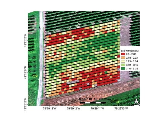
Graphical Abstract

1. Introduction

Grapes grown on over 920,000 acres (~372,000 hectares) in the United States for wine, raisins, fresh market, and juice products have a multi-billion dollar production value [1]. Macro- and micronutrients are often applied as fertilizers in vineyards to optimize the vine size and fruit quality. Nitrogen, in particular, is an important component of proteins, nucleic acids, and chlorophyll [2]. It is commonly applied to vineyards, since it plays a major role in the growth and development of shoots and leaves, which photosynthesize to support the subsequent fruit development. Too little N results in depressed vegetative growth, while too much results in excessive vegetative growth [3]. Therefore, an accurate and precise assessment of grapevine leaf blade or petiole (i.e., leaf stem) contents of nutrients is required to guide the judicious application of fertilizers to optimize both the quantity and quality of grapes. Additionally, the application of appropriate amounts of N, as well as other nutrients, will allow for minimized detrimental impacts in the vineyard (e.g., soil acidification), as well as off-site impacts (e.g., groundwater pollution and the eutrophication of nearby waterways) [4].
While nondestructive remote sensing applications have been developed to improve the nutrient management of other crops, the current methods of collecting and measuring grapevine nutrients are destructive, time-consuming, and costly (~$25 per sample). Typically, a grower will manually collect leaf blades or petioles from many vines, combine them to form one representative sample of a vineyard block several acres in size, and mail the sample to a lab for analysis. This standard practice is spatially inadequate to effectively map nutrient deficiencies, particularly in vineyard blocks with a high variability in the soils and/or vine growth. Rather than applying localized fertilizer amendments, growers use their sparse data to guide their application of fertilization to many acres of their vineyards with a common prescription, resulting in suboptimal growth and unnecessary leaching and runoff of nutrients.
An increase in the affordability of unmanned aerial system (UAS) imaging capabilities has prompted several studies estimating the nutrient status (especially N) in a variety of crops using these platforms. These include hyperspectral and multispectral imaging systems used for nitrogen estimations in wheat [5,6], rapeseed [7,8], barley [9], rice [10,11,12], corn [6], potatoes [13], and sunflowers [14]. The advantage of a UAS platform is the ability to obtain high spatial and temporal resolution at a low cost [15], while the disadvantage is related to difficulty in scaling the results to larger areas.
UAS-based crop nutrient studies and all alternative field, lab, airborne, satellite, or synthetic spectral studies use a variety of methods to model the nitrogen status. These can include parametric regressions with sets of bands or derivative spectra; vegetation indices (VI); spectral transformations (such as continuum removal [16]); chemometric methods like the principal component analysis (PCA) [17]; partial least squares regression (PLSR) [18] and stepwise multiple linear regression (SMLR) [19]; or machine learning methods like random forest (RFR) [20], support vector machines (SVM) [21], and gaussian process regression [18]. Overall, these studies utilize a variety of experimental designs, predictor variable selections, nutrient measurement standards, regression or classification methods, prediction error estimation techniques, and vary in their reported accuracies. However, all of these methods face a number of challenges inherent to estimating the nutrient status from spectral data, highlighted in the recent review papers by Berger et al. [22] and Fu et al. [23] on the spectral monitoring of crop nitrogen.
The major impediments to finding correlated spectral responses to vegetation traits using hyperspectral data are the redundancy in their high data dimensionality and the propensity of a limited sample (i.e., fewer than the number of potential predictor variables) to cause overfitting, preventing the development of robust generalized models [24]. This is why many studies use well-known or empirically derived vegetation indices consisting of just a small number of bands [25] while others combine a variety of machine learning feature selection methods to build models utilizing only the most target-relevant features [26,27]. Feilhauer et al. [28] found that an ensemble of SVR, RFR, and PLSR machine learning methods achieved consistent wavelength selections between different datasets in good agreement with known spectral absorption features compared to the standard partial least squares regression technique for spectral band selection related to leaf biochemistry [29].
The nitrogen content has been studied more than any other nutrient, mainly because of its universal importance to crop productivity. Its abundance in foliage occurs primarily in proteins and chlorophylls [30]. However, the known nitrogen absorption features are relatively weak [31] and overlap with the dominant water absorption features and abundant signatures of the other organic compound constituents (cellulose, lignin, protein, oil, sugar, starch, etc.) [32]. In fact, VIs utilizing wavelengths in the visible and near-infrared (VNIR) regions of the spectrum, related to chlorophyll absorption and red-edge position, are more widespread than SWIR-based nitrogen indices, designed to sample specific N-H stretching and bending overtones [22,23]. Unfortunately, the use of the chlorophyll content as a proxy for nitrogen is limited by seasonal variations and can be misconstrued when other deficiencies occur [33]. For example, Rustioni et al. [34] found that iron, magnesium, nitrogen, and potassium deficiencies all produced chlorotic symptoms in the grapevine canopy. The review of nitrogen monitoring studies conducted by Berger et al. [22] recommended including a combination of the VNIR and SWIR domains to improve the models for nitrogen by sampling both the chlorophyll-N and protein-N-related spectral regions.
In a recent study, Camino et al. [35] used airborne combined VNIR and SWIR imagery to model the nitrogen concentration in wheat. They found that indices modified to use reflectance at 1510 nm (N-H stretch, first overtone) in the place of 670 nm resulted in higher correlations than traditional canopy structural indices (e.g., R2 of 0.69 vs. 0.63 for the modified chlorophyll absorption reflectance index—MCARI). Additionally, their optimal model paired solar-induced chlorophyll fluorescence with the biophysical canopy parameters estimated from physical models [36,37], achieving a leave-one-out cross-validation (LOOCV) root mean squared error (RMSE) of 0.2% nitrogen in samples ranging from 2 to 5% nitrogen. Nasi et al. [17] combined UAS-based hyperspectral imagery and canopy height measurements derived from an RGB camera to model the nitrogen content in barley with a LOOCV RMSE of 0.59% nitrogen in samples ranging in nitrogen contents from 1.71 to 4.23%. In grapevines, specifically, Friedel et al. [25] found that the red-edge inflection point index (REIP) had the lowest RMSE (~0.17% nitrogen by dry mass in samples ranging from 2.18 to 2.58%) when comparing the vegetation indices derived from handheld spectral data. Conversely, Omidi et al. [26] determined the optimal handheld spectral bands of the leaf samples centered at 596, 611, 401, 1619, 825, and 1386 nm to be the most important for the classification of high and low nitrogen content grapevines. Moghimi et al. [38] modeled the nitrogen content for the same vines using UAS-based five-band multispectral imagery with a RMSE (hold-out test set) of 0.23% nitrogen in samples with contents ranging from 2.25 to 4.25% nitrogen.
In the late summer of 2020, we began a multiyear study using UAS-based imaging spectroscopy (hyperspectral imaging) to determine the optimal wavelengths to estimate the N content and other essential macro (P, K, Ca, and Mg) and micro (B) grapevine nutrients in upstate New York, USA. The novel use of UAS spectral imaging serves as a practical bridge between more typical in situ spectral sampling and UAS multispectral imaging. This paper details our first season of observations, including both VNIR and SWIR spectral imagery coincident with leaf and petiole sampling for a nutrient lab analysis occurring at the veraison growth stage (start of rapid fruit ripening). At this late growth stage, the concentrations of some nutrients, like potassium, are more stable and correlate with the vine performance than at bloom, but near full bloom sampling is typically better for assessing the N and a majority of plant nutrients [39]. Future efforts will include cumulative data from investigations of both growth stages over multiple seasons to assess the nutrient status and determine the optimal bands and growth stages for image acquisition.
The study was motivated by the need for an accessible and data-driven solution to quantifying the grapevine nutrient content with the goal of better guiding management. There is a potential to capitalize on the low cost of high-resolution multispectral imaging on small UAS (sUAS) by tailoring imaging systems with appropriately tuned bands for each nutrient. The specific objectives of this study are to (i) build predictive regression models using optimized combinations of VNIR and SWIR wavelengths, determined with ensemble feature selection, (ii) compare our results to PLSR, and (iii) assess the practicality of monitoring individual nutrients and create nutrient specific benchmarks for comparisons with future observations.

2. Materials and Methods

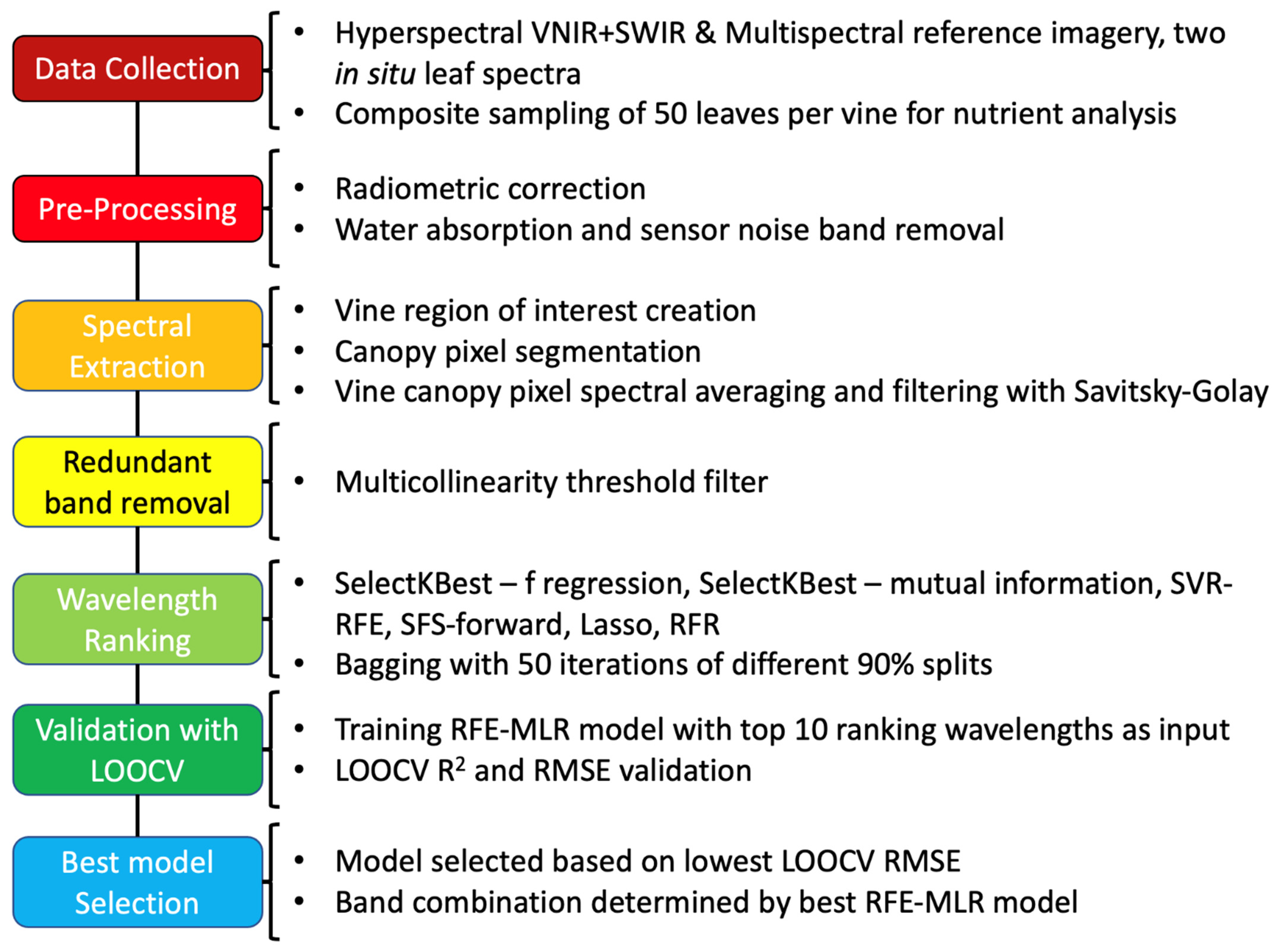
The complete process, including data collection, preprocessing, and data analysis, is summarized in a flowchart in Figure A1.

2.1. Study Area

The experimental study area was a 0.43-ha (1 acre) Concord grape (vitis labruscana) vineyard block located within the Cornell Lake Erie Research Extension Laboratory (CLEREL) in Portland, NY, USA. The block contains 23 rows of grapevines, each 72.5 m long, with 29 consecutive grapevines, as shown in Figure 1. From north to south, the block was designed to induce five rows each of nitrogen-deficient, control, potassium-deficient, and low-pH grapevines, with a single buffer row between each of the four treatment zones. The control rows received 56 kg/ha (50 lb/acre) of N fertilizer, 2242 kg/ha (1 ton/acre) of lime, and 224 kg/ha (200 lb/acre) of potash. The same prescription was applied to each of the deficient rows, with some specific exceptions. In addition to omitting N fertilizer in the N-deficient rows, weeds were allowed to grow between the rows to allow for competition with the vines for the available N. In the K-deficient rows, a second dose of lime was used to drive up the soil pH, and no potash was applied. Finally, in the low-pH rows, 1681 kg/ha (1500 lb/acre) of ground sulfur was used in place of lime to decrease the soil pH from 6.0 to 4.5.

2.2. Aerial Imaging Systems

The imaging data were captured with two UAS platforms via visual and near-infrared (VNIR) and short-wavelength infrared (SWIR) push-broom style (hyperspectral) imaging spectrometers. The VNIR imagery was collected with a Headwall Photonics Nano-Hyperspec imaging spectrometer (272 spectral bands from 400 to 1000 nm), while the SWIR imagery was collected with a Headwall Photonics Micro-Hyperspec M384 imaging spectrometer (170 bands from 900 to 2500 nm). Each spectrometer was mounted on a separate DJI Matrice 600 Pro UAV, each paired with an Applanix GPS/IMU for a pixel georeferencing accuracy of 1–3 cm. The VNIR UAS payload also included a MicaSense RedEdge-M 5-band (blue, green, red, red edge, and near-infrared) multispectral camera for both the reference imagery and further investigations. The multispectral imagery results in a cleaner mosaic for scene display purposes than the push-broom style flight line spectral imagery.

2.3. Imaging Campaign

The Rochester Institute of Technology (RIT) drone team collected imagery of the study area on 6 September 2020 between 10:30–11:30 a.m. EST. At the time of flight, the sky conditions were fair, with no clouds blocking the sun throughout the flights, and the wind was below 5 m/s. The flight altitude for the VNIR and SWIR flights were 48 m and 30 m, respectively, each flying at 2 m/s to achieve a ground sampling distance (GSD) of approximately 3 cm in both hyperspectral modalities.

2.4. Sampling Plan

The CLEREL team collected grapevine petiole and leaf samples for the nutrient analysis from the study area on 4 September 2020. Unfortunately, the timing of optimal sampling for the veraison growth stage (start of rapid fruit maturation) and the weather prevented same-day sampling and imaging campaigns. This could raise concerns, because this work explores relationships between the canopy imagery and nutrient levels from samples obtained two days apart. However, during veraison, the N and K levels are relatively stable compared to the bloom growth stage [39], but the same is not true for other nutrients like Mg [40].
The samples were collected from 100 individual vines in the vineyard block, including 25 vines from each subblock, shown in Figure 1. For each vine, we collected a composite sample of 50 leaf blades separated from their petioles. The leaf samples were washed in deionized water and dried in an oven at 60 °C until the sample weight stabilized, ground through a 1-mm sieve, and sent to the Penn State Agricultural Analytical Services Laboratory for a standard tissue nutrient analysis using acid digestion and multielement analysis by inductively coupled plasma (ICP) emission spectroscopy [41]. The final nutrient results were for six nutrients of interest to viticulture management (N, P, K, Ca, Mg, and B) for each vine.
In addition, two leaf sample spectra were taken of each study vine using a Spectra Vista Corp. (SVC) field spectroradiometer (model HR-1024i) with a leaf clip coincident with the UAS flights. The instrument captures spectral data from 335 to 2500 nm in 987 bands. The dataset was too limited to be considered representative of individual vines but was a useful reference to compare with the lower spectral resolution UAS-based spectral imagery (see Discussion and Figure 5).

2.5. Data Preprocessing

The data preprocessing steps included radiometric correction, vine region-of-interest (ROI) creation, vegetation segmentation, and spectral extraction.

2.5.1. Radiometric Correction

The VNIR and SWIR instruments both captured spectral imagery of two sets of black, dark gray, medium gray, and light gray calibration panels laid out on the west side of the vineyard block. The calibration panel spectra from both the VNIR and SWIR imagery were extracted using ENVI version 5.5 [42]. These panels had well-characterized ground truth reflectance spectra collected via a Spectra Vista Corporation (SVC) spectroradiometer (model HR-1024i) that were used to convert the radiance flight imagery into reflectance. The Empirical Line Method (ELM) [43] tool in ENVI was used to determine the relationship between the calibration panel UAS radiance spectra and their true reflectance spectra and determined the linear coefficients to convert between radiance and reflectance at each wavelength. This process removes both the solar irradiance and atmospheric path radiance. However, this cannot be reliably accomplished at all SWIR bands, due to the deep water absorption features where the SWIR detector did not detect photons. Thus, we removed the spectral bands in the water absorption band regions 1340–1470 nm, 1790–2020 nm, and from 2365 nm onward to avoid the possibility of nonsensical ELM coefficients. Additional wavelengths were removed near the edges of both instruments’ wavelength ranges where sharp drop-offs in signal-to-noise (SNR) occurred. These wavelengths were those at <460 nm and >900 nm for VNIR and <950 nm and >2270 nm for SWIR.

2.5.2. Vine Image Extraction

Rectangular images were extracted for each grapevine, measuring 2.5 m long by 3 m wide, prior to canopy segmentation. No field markers were used to mark the study vines, but the row length was divided into evenly spaced vines based on the known consistent vineyard block row length and vine spacing. The row center lines were created using the QGIS (V. 3.12) advanced digitizing tool for precise length and angle-of-row center line. The vector geoprocessing tools were used to create a buffer from the row center line resulting in a polygon row feature, then divided with the split polygon plugin to evenly separate the 72.5-m-long row into 29 vine polygons. The vine vector feature shapefiles were then imported as ENVI ROIs for extraction using the ENVI Subset Raster task. Finally, the Spectral Python—SPy [44] library was used to load the ENVI hyperspectral vine imagery into NumPy arrays for all further image processing. The vine extents for the 100 study vines are subset from their consecutive neighboring vines in Figure 1.

2.5.3. Canopy Segmentation and Spectral Extraction

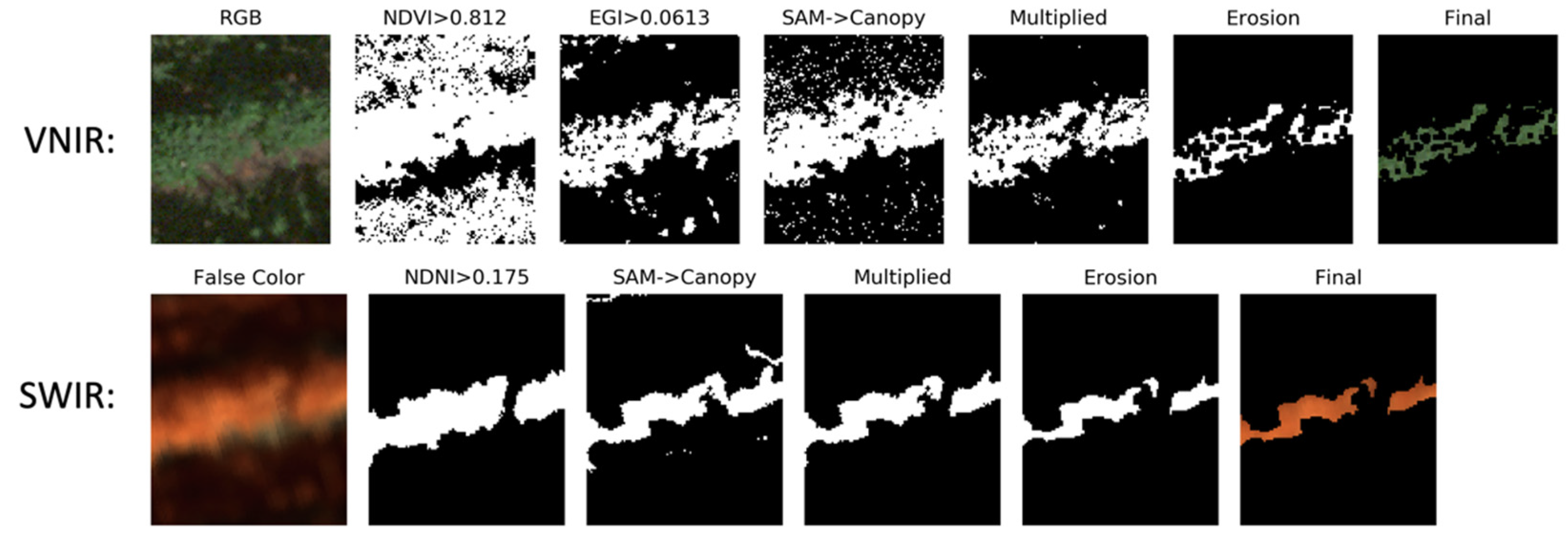
A combination of techniques was used to separate the grapevine canopy pixels from the neighboring soil, shadow, and grass pixels. Grass was allowed to grow in the spaces between the nitrogen-deficient rows to further induce deficiency in the grapevines, which complicated the efforts to use a single vegetation index threshold to mask the grapevine canopy alone. The final canopy mask for VNIR imagery was a combination of a normalized difference vegetation index (NDVI) threshold, an excessive greenness index (EGI) threshold, and spectral angle mapper [45] (SAM) binary masks. For SWIR, a combination of a normalized difference nitrogen index (NDNI) threshold and SAM binary masks was used. The vegetation index mask(s) were multiplied and combined with the SAM mask to generate a primary mask for the vegetation segmentation of each vine. Further, the application of a morphological erosion operator (3 × 3 matrix of ones) to the primary mask removed mixed pixels from the canopy edge [46]. The results of each masking step are shown in Figure 2.
A threshold value for each vegetation index was chosen using an automated process of determining peaks and troughs in vegetation index pixel value histograms. The histograms represent the frequency of the vegetation index values for all of the non-nitrogen-deficient subblock vines to avoid a skewed threshold due to an abundance of grass pixels. For each vegetation index, a threshold was selected halfway between the detected peak vegetation signal corresponding to the grapevine canopy and the neighboring trough. For the spectral angle mapping approach, endmember spectra were extracted from manually selected canopy, grass, soil, and shadow pixels. Spectral angles with each of the endmember spectra were computed for all the image pixels using the SPy library spectral_angles function [44]. The spectral angle is an N-dimensional angle found by treating spectra as a vector in a space having a dimensionality equal to the number of bands. Individual pixels were classified as canopy pixels if their spectral angle with the canopy endmember spectra was smaller than with the other endmembers.
Finally, the mean canopy spectra of each vine image were extracted using the eroded canopy masks. A Savitzky–Golay (SG) filter (scipy.signal savgol_filter) was used to smooth the grapevine spectra using a window length of 15 bands [47]. The optimal window length was found by inspecting the Fourier-transform frequency spectra of both the sample vine’s raw spectrum and various window-length SG-filtered versions of the spectra. This reduced the high-frequency noise but maintained the pertinent spectral features. Further, the differences between the raw spectra and their corresponding filtered spectra were not to exceed the standard deviation of all the vine spectra at each wavelength. This requirement ensured that the chosen window length preserved the spectral variations between the vines. All SG-filtered grapevine spectra were then stored in a pandas DataFrame for the remaining analysis.

2.6. Data Analysis

A standard method was used to optimize the regression models for each of the 6 nutrients. For each model, this included an initial reduction in the independent variables to decrease the computation time and mitigate the spectral band multicollinearity issues. Next, the remaining features were ranked with an ensemble of filter, wrapper, and embedded feature rankers, and an optimal combination of the features drawn from the 10 highest-ranking features was determined. Feature selection was used, as opposed to feature extraction, for dimensionality reduction, because feature extraction methods like PCR require a new feature space where the reduced number of features is some combination of all the original input features [48]. Feature selection, in contrast, allowed us to achieve our objectives aimed at devising a multispectral sensor with a smaller subset of optimized bands. Feature selection also maintains the physical reflectance measurement at each wavelength and its relation to the grapevine nutrient status, which is desirable for consistent translation to a multispectral sensor.

2.6.1. Multicollinearity Assessment

A correlation threshold of 95% was used to reduce the number of redundant features and mitigate the multicollinearity. For any pair of bands that were linearly correlated with each other above 95%, the band having the lesser correlation with the target nutrient was removed [49]. This reduced the number of bands for subsequent use in the ensemble feature selection. For example, this step reduced the number of bands from 299 to 27 for the leaf N content dataset used in this study.

2.6.2. Ensemble Feature Selection Rankers

The ensemble feature selector used a combination of six feature rankers, similar to Omidi et al. [26] and Moghimi et al. [46]. Using a multimethod ensemble combines the advantages and disadvantages of a diverse set of methods to rank features. This arguably will yield a more reliable generalized set of spectral regions associated with leaf biochemistry [28]. For filter rankers, the sklearn.feature_selection (version 0.21.3) SelectKBest univariate feature selector was used with both the linear regression test (f_regression) and mutual information regression (mutual_info_regression). SelectKBest can be used to reduce a dataset into user-defined k features based on their ranking or to report the complete rankings of all the input features using a number of possible classification or regression scoring functions. f_regression scoring ranks each feature based on their F-scores and p-values with the target variable. Mutual information regression scores each feature based on a measurement of the nonparametric dependency with the target variable [50,51]. A linear kernel support vector regression recursive feature eliminator (SVR-RFE) [52] and a forward sequential feature selector (SFS-forward) [53] wrapper for standard multiple linear regression (MLR) were used for the wrapper methods. Finally, the least absolute shrinkage and selection operator (Lasso) [54] and random forest regression (RFR) [55] were included as the embedded methods to rank the input features.

2.6.3. Ensemble Feature Selection Method

The remaining data, i.e., after removing the bands with the multicollinearity assessment, were fed into an ensemble feature ranking loop for 50 iterations of the feature ranking, using a different random split of 90% of the data for each iteration. After the ranking loop completed, the 50 iterations of the six feature rankings (300 rankings for each band) were averaged to determine the overall band rankings. This is essentially bootstrap aggregation, or bagging of the feature ranks to improve the stability and reduce the variance of the ranking results. Leave-one-out cross-validation (LOOCV) scores were used to assess the optimal number of bands. To do this, an RFE wrapper selected the subsets of the top 10 remaining bands from 1 to 10, calculating the LOOCV-adjusted coefficient of determinations (R2) and root mean squared errors (RMSE) for the MLR-RFE models. The minimum LOOCV-RMSE score for the explored combinations defined the optimal number and combination of the top-ranking bands used to construct the final model for each nutrient.

2.6.4. PLSR Comparison

For all nutrients, the results were compared to the standard PLSR approach, similar to Feilhauer et al. [28]. First, redundant features were eliminated, as described in Section 2.6.1. While PLSR is not itself a feature selection implementation, several methods to select features based on PLSR results have been proposed and are commonly used [56]. PLSR transforms the input wavelength features into latent variables that are linear combinations of the original features and are statistically independent from one another [56]. Regression is then performed between the resulting latent variables and the target variable.
The PLSR method optimized the LOOCV scores via an exhaustive exploration of the number of latent variables less than 10 and the optimal number of input features used to create the latent variables. The number and order of the increasing input features tested were filtered by the band-specific regression coefficients or the coefficients mapping each input variable to the number of latent variables being explored. The regression coefficients are a standard output of sklearn.cross_decomposition PLSRegression implementation.

3. Results

The LOOCV score results for the ensemble and PLSR methods for leaf blade nutrients are shown in Table 1, along with the final number of bands selected in each case. The PLSR method resulted in slightly higher adjusted R2 for all the models, but it did not distinctly outperform our ensemble method in terms of the RMSE in all cases. The majority of the ensemble models required fewer wavelengths to achieve comparable RMSE. For example, the nitrogen models exhibited identical RMSE, but the ensemble model used half the features of the PLSR model. In fact, in several of the PLSR models, the optimal number of wavelengths was the maximum imposed by our limit of 10 latent variables and 10 top-ranking wavelengths.
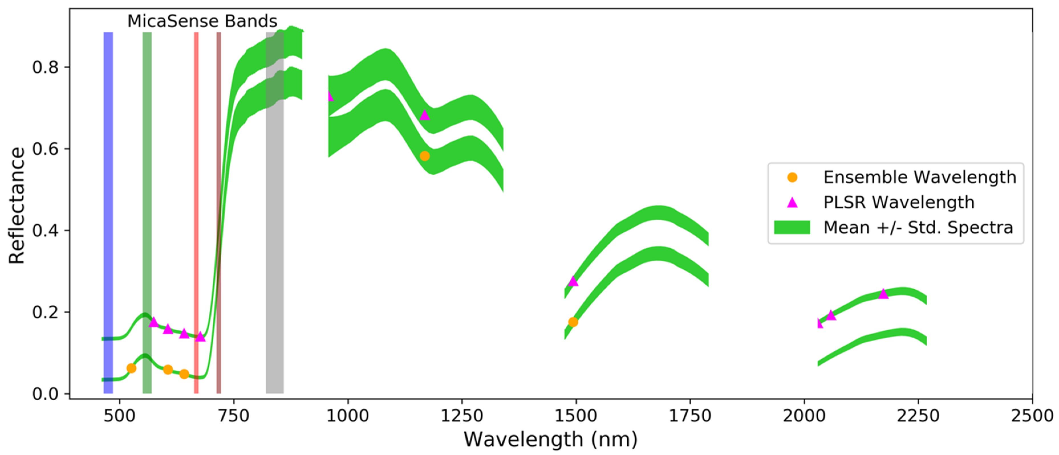
Figure 3 shows the selected wavelengths for both methods pertaining to the nitrogen content in relation to the average grapevine spectra for reference. A complete record of all the selected wavelengths for all the nutrient models are included in Appendix A. The ensemble and PLSR models for nitrogen shared wavelengths at 606, 641, 1168, and 1494 nm. The ensemble model used just one additional blue–green wavelength, while the PLSR model used two additional wavelengths in the visible range (red and green) and four additional wavelengths in the SWIR range.
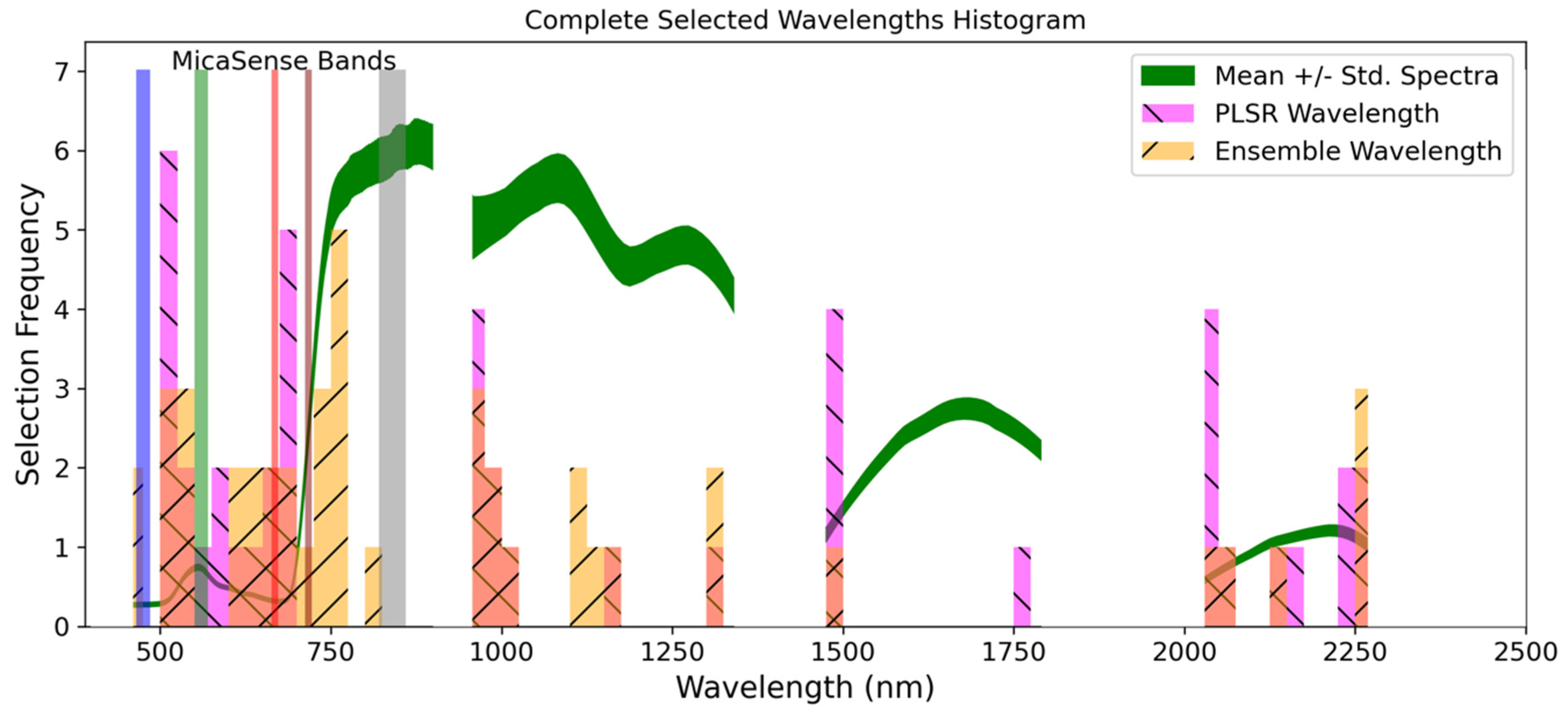
The selected wavelengths are plotted for all the nutrients as a histogram in Figure 4 to show the frequency of wavelengths chosen from regions of the vegetation spectrum in 25-nm-width bins. The histogram for the ensemble and PLSR methods is displayed along with the average spectra and vertical bars denoting the MicaSense RedEdge five-band multispectral camera bands for reference. A number of observations can be made based on Figure 4: (i) with the exception of blue, the selected bands cover the visible region of the spectrum, while there are distinct peaks in the blue–green and deep red for both methods; (ii) an orange peak and peak at the top of the red edge are also present for the ensemble method; (iii) there is a lack of bands selected in the NIR plateau range, especially around the typical NIR multispectral band centered at 840 nm; and (iv) the selected wavelengths in the SWIR region favored the edges of the strong water absorption features, although the PLSR method also selected wavelengths at a high frequency near 2125 nm.

4. Discussion

4.1. Methodological Considerations

The multicollinearity threshold filter to eliminate redundant wavelengths was effective at reducing the initial number of bands (299 bands remained after removal of the noisy and water absorption features) to less than 30 in all cases before applying the feature selection methods. A more extensive search could explore varying the multicollinearity threshold to increase or decrease the number of redundant wavelengths allowed into the selection procedure. However, a more lenient threshold will increase the computation time.
The ensemble feature ranking followed by MLR-RFE method and the standalone PLSR method each achieved comparable performances in terms of the LOOCV-RMSE, but both may be further improved by exploring alternatives. For example, in the case of ensemble ranking, alternative rankers might prove superior, or the recursive elimination of rankers might be used to optimize the regression results [26]. Additionally, other parent regression methods, such as SVR or RFR, may yield lower RMSE than MLR. This was not true in the initial testing of the ensemble method for nitrogen, so MLR was used to improve the computational speed when testing the method on several nutrient targets. Several alternative methods of feature selection using PLSR that could improve selection stability were presented by Mehmood et al. [56].
The maximum number of wavelengths in each selection method was limited to 10, because this is a practical limit for the existing sUAS multispectral systems. However, an even stricter limit may be appropriate for tailoring a set of bands to a particular platform.
Ultimately, ensemble feature selection has been found to be more stable than PLSR when using spectral data to assess the leaf biochemistry across multiple datasets [28]. Even if the regression scores were less accurate on a particular dataset, we expect the wavelengths selected with the ensemble method to be more stable and accurate across different grapevine datasets.

4.2. Regression Model Performance

Obtaining only 100 samples from a single growth stage and season proved insufficient to determine the regression models with high correlations between the grapevine nutrient contents and variations in the canopy spectra using either the ensemble or PLSR selection methods (see Table 1). This is likely a result of the similarity in the spectral responses due to various nutrient stresses and the variety of deficiencies that resulted in the study sample. In fact, the major limitation of using vegetation spectra for individual nutrient assessments is that most stresses (both abiotic and biotic) in vegetation result in a decreased chlorophyll concentration in the leaves [34]. As a result, multiple correlated nutrient deficiencies may exhibit a mixed response, diminishing the correlations to any individual nutrients at the relevant spectral regions. Due to this, and a lack of individual nutrient regression models beyond nitrogen to compare to in the literature, we have limited the further discussion of specific wavelength selections and model results to nitrogen. Some further comments concerning the physiological significance of the overall wavelength selections are included in Section 4.4.
Despite an increased use of UAS imagery in viticulture [57], few studies have been conducted to assess the grapevine nutrient status in vineyards and fewer with remote sensing imagery [58,59,60], specifically. Most studies involving the nutrient content in vineyards limit regression modeling to the associated chlorophyll content [59,60] or nitrogen [38,60]. Moghimi et al. [38] recently observed grapevine canopy reflectance with a multispectral imager aboard an unmanned aerial system (UAS) and were able to estimate the N content to within 0.23% among 150 samples with 2–4% N. Similarly, using UAS-based multispectral imagery, Retzlaff et al. [60] found an RMSE of 0.26% N for samples with 1.5–3.5% N. Our slightly improved RMSE of 0.17% for leaf nitrogen among samples with a similar range of N contents suggests that there is only a modest potential for a tuned multispectral system to significantly improve the nitrogen status monitoring. Indeed, the R2 found in these analogous studies (Moghimi: R2 = 0.56 and Retzlaff: LOOCV R2 = 0.52) were slightly higher than the model presented here (LOOCV R2 = 0.44). While the N range of 2–4% is appropriate for different cultivars and regions [3,61,62], ground truth sampling at a much larger scale (>100 samples) may be necessary for the greater refinement of optimal bands to improve the nitrogen regression model accuracy.

4.3. Nitrogen Wavelength Selections vs. Spectral Features

The selected wavelengths of both methods indicate that differences between the spectral responses of low and high nitrogen contents are the result of biochemical changes related to the leaf chlorophyll concentrations. Table 2 shows the ensemble and PLSR-selected wavelengths for nitrogen, along with the nearby known strong absorptions related to chlorophyll, nitrogen, proteins, and water. In particular, the selection of SWIR bands near to the nitrogen-related absorption features at 1510 nm and 2180 nm were noted as strong absorptions by Curran [32]. The chlorophyll absorption-related wavelengths in the VNIR region were consistent with the most frequently selected bands found by Fu et al. [23] in their review of the crop nitrogen status using hyperspectral remote sensing. Our selection of 606 nm fell right between 596 nm and 611 nm, a spectral region noted by Omidi et al. [26] in their study of grapevine leaf handheld spectral data using an ensemble ranking method for the classification of nitrogen deficiency.
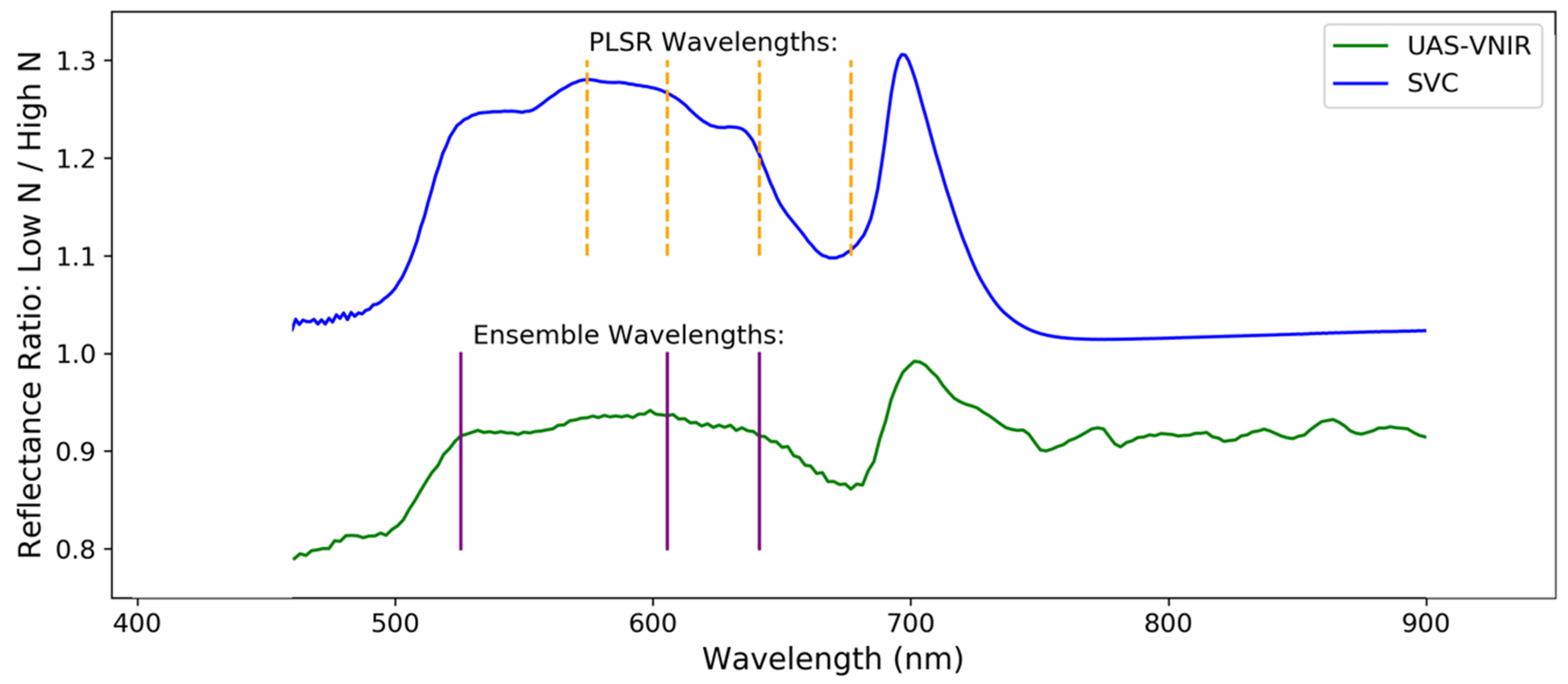
Figure 5 shows the VNIR spectrum of a typical nitrogen-deficient vine divided by a typical healthy vine spectrum to emphasize the spectral regions where nitrogen-deficient vines differ from healthy vines using an approach similar to Friedel et al. [25]. The green ratio spectrum (lower) is the ratio of the average spectra extracted from UAS hyperspectral imagery of the ten-lowest and ten-highest nitrogen content vines. The blue ratio spectrum (upper) is the equivalent gathered with a handheld SVC field spectroradiometer using a leaf clip. Vertical lines mark the wavelengths selected by the ensemble and PLSR methods from the UAS data separated from each other for clarity.
While the handheld spectra were limited to just two leaf spectra per vine, they have considerably improved radiometric properties, because the leaf clip uses its own standard light source and internal calibration target. If the spectra of the healthy and nitrogen-deficient vines were equivalent, the ratio spectrum would be a horizontal line with a value of 1 at all wavelengths. However, there were distinct differences between the average healthy and nitrogen-deficient spectra, expressed as deviations from 1, in their ratio spectrum. This is well-represented in the handheld ratio spectrum but less clear for the UAS-derived ratio spectrum, which was attributed to slight differences in the illumination conditions during the UAS flight lines over the healthy and nitrogen-deficient vines and the calibration panels (more on this in Section 4.5). Nevertheless, both ratio spectra shared a similar overall trend and indicated relative increases in the reflectance for the nitrogen-deficient vines from 500 to 675 nm and at 700 nm.
The overall increase in reflectance at the mid-visible wavelengths was attributed to reduced chlorophyll absorption. In particular, the reduced absorption is centered at green–yellow wavelengths, and blue absorption is less diminished by a low N content than red absorption, similar to the findings of Moghimi et al. [38] and Rustioni et al. [34]. This can be explained by a relative stability or increase of carotenoids and greater decrease in chlorophyll b compared to chlorophyll a [34]. Another result of a low N concentration is the known shift in the red-edge position to shorter wavelengths associated with the decline in chlorophyll absorption [63].

4.4. Overall Wavelength Selection Spectral Regions

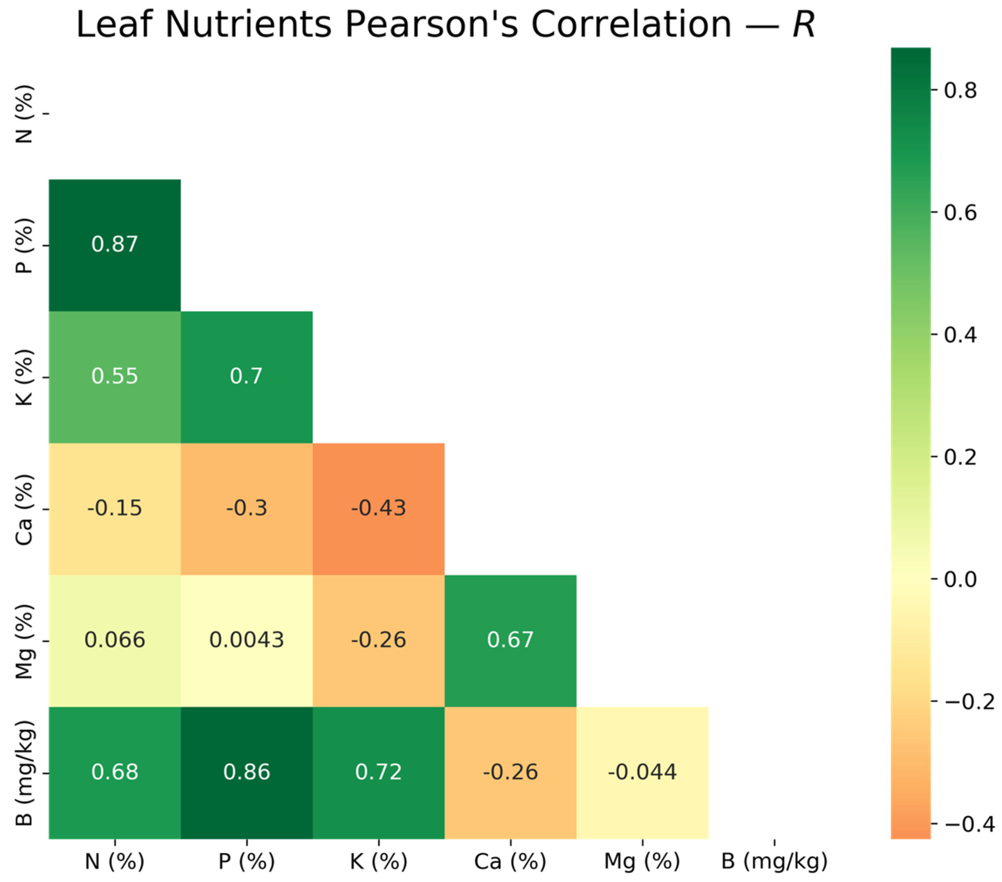
The frequency of the spectral regions selected for the six nutrient models suggests that the visible spectrum may be most informative for quantifying grapevine nutrient deficiency during veraison. This is consistent with Rustioni et al. [34], who found that iron, magnesium, nitrogen, and potassium deficiencies all exhibited chlorotic symptoms in the grapevine canopy. The only physiological associations identified between the selected spectral bands and nutrients beyond nitrogen were with an abundance of bands in the visible and red edge. The wavelengths around 700 nm (red edge) and those from 530 to 680 nm (green to red) are generally associated with stress-induced chlorophyll deficiency [64] and can be due to a variety of nutrient deficiencies (N, P, K, Ca, Mg, and B) [34,39,65]. This is illustrated by the high frequency of the band selections in the visible region of the spectrum in Figure 4 and the specific bands noted in Table A1. In fact, much of the nutrient content was correlated among the samples, as shown in the heatmap in Figure 6. In particular, N, P, K, and B were mutually correlated and distinct from correlated Ca and Mg, similar to the findings of Gil-Pérez et al. [58] in airborne vineyard imagery. This emphasizes the reality of a mixed spectral response due to multiple potential nutrient deficiencies. However, the peaks in the selected wavelength histogram (Figure 4) did occur outside of the typical bandwidths of a five-band VNIR multispectral camera. This suggests that a multispectral system with fewer than 10 bands could potentially be better optimized for individual nutrient monitoring once the signals from individual nutrients are isolated in a larger dataset.
While many bands were selected in the SWIR range, these bands will be highly variable due to the differences in water stress and imperfect atmospheric compensation. The higher frequency of selected bands near the edges of the removed spectral bands is particularly worrisome. In multiple linear regression models with limited samples, these particularly variable bands may slightly improve the regression by chance while not actually being related to the target nutrient. Some studies of nitrogen contents using hyperspectral data obtained with handheld spectrometers have demonstrated improvements with nitrogen-related SWIR bands [66,67]. However, SWIR bands may be impractical and cost-prohibitive to the development of a multispectral sensing UAS solution for the grapevine nutrient status, given the need for more expensive detector materials and even cooling requirements [23].

4.5. Future Research and Potential Improvments

A major potential improvement to achieving optimized spectral models from hyperspectral imagery is the implementation of a hyperspectral downwelling light sensor. The current practice for radiometric correction is to use field-deployed calibration panels with well-characterized spectral properties as a reference in UAS imagery. The calibration panels cannot be present every moment the push-broom spectrometer is traversing the vineyard, so any variation in the illumination conditions that occurs between visits to the panels results in a radiometric correction error. Unfortunately, the best that can be done to mitigate this error is to manually choose the panel spectra most closely representing the conditions present during each swath of imagery when applying the empirical line method. A downwelling light sensor that obtains spectral data of the sky both spatially and temporally coincident with the imaging spectrometer is an ideal solution to mitigate this issue and improve UAS spectral imagery acquisition.
Future investigations should consider the impact of flight altitude on vineyard nutrition monitoring. The current experiment was designed to achieve an optimal GSD (~3 cm) and spatial coverage (one acre) within a flight time of about 15 min by using an oversized UAS payload designed for a variety of scientific endeavors. However, typical sUAS multispectral sensor platforms likely need to fly higher and cover more area (possibly several acres per hour) than the UAS used in this study to be practical. Once the optimal wavelengths are consistently identified, constraints on the required GSD (having sensor dependence on the altitude) should be explored.
Furthermore, rather than identifying bands that are most correlated with each nutrient, as these may be correlated with a number of nutrients, it may prove more effective to consider bands or indices that more effectively distinguish between and classify individual nutrient deficiencies. This strategy was recently explored by Debnath et al. [65] to classify deficiencies in grapevine leaves using the hyperspectral imaging of individual leaves in a lab. Future investigations might also benefit from using one of the consistently selected bands found here to normalize the input spectra and conduct feature selection from the resulting normalized band ratio spectra.
Future studies should continue to explore the consistency of SWIR band selections and their importance to grapevine leaf nutrients. However, the performance of VNIR-only band selection should be compared against combined VNIR and SWIR results [22,67]. If the SWIR bands provide inconsistent results and limited improvement, a VNIR system may be more practical, given its reliance on affordable silicon (Si) as a ubiquitous detector material.
Further investigation is also required to better characterize the relationship between grapevine leaf nutrients and the spectral response, particularly for nutrients beyond nitrogen. These relationships should be established at both the leaf level, using handheld spectrometer data with a leaf clip, and the canopy level, using UAS spectral imagery. Canopy-level spectra are more complex due to the structural trait impacts, atmosphere, soil, and non-leaf plant parts influencing the spectral response [68]. Nutrients that produce weaker spectral responses may be found in the leaf-scale spectra but are more difficult or impractical for identification at the canopy scale [16,69]. While a dried nutrient sample lab analysis is currently the standard practice guiding vineyard management [39], future investigations might consider alternative methods to sample nutrient data in situ to provide more consistent comparisons with remote sensing imagery. Regardless, this work and additional studies will provide useful benchmarks for comparisons and for reaching the goal of identifying consistent wavelengths for nutrient-specific management protocols and sensors.

5. Conclusions

The results of this Concord vineyard study showed that ensemble feature selection can identify wavelengths providing comparable prediction accuracy to PLSR feature selection for predicting key micro- and macronutrients in vineyard management. Many of the selected wavelengths for the grapevine leaf nitrogen content were consistent with the known absorption features related to nitrogen. These included well-known associations in the VNIR range related to the chlorophyll concentration, as well as SWIR bands related to nitrogen absorption in proteins. However, the regression model correlations for all the modeled nutrients were relatively low (LOOCV R2 < 0.50), thus indicating that a much larger dataset or alternative method is necessary to isolate the spectral response contributed by individual nutrients. Due to the correlations among individual nutrients and an overall common chlorotic spectral response, little can safely be speculated about the other nutrients (P, K, Ca, Mg, and B) based on their individual band selections. Further testing of the ensemble method with new datasets is needed to confirm the spatial and temporal consistencies of the wavelength selections and determine if there is improved model generalization and performance compared to PLSR. We concluded that the multicollinearity threshold and ensemble feature ranking approaches are promising methods that should be added to spectral preprocessing procedures to dramatically reduce the number of features for initial regression modeling. These methods should be explored further with new datasets to refine the informative bands for grapevine nutrient monitoring with optimized UAS multispectral sensing. This approach in general bodes well for the transition from research-grade hyperspectral imaging to the more affordable, operational use of multispectral sensing for precision agriculture in vineyard management. Regardless, the nitrogen-optimized bands selected here from hyperspectral imagery did not definitively outperform other studies using the standard multispectral imagery [38,60]. In fact, multispectral imagery may prove sufficient for nutrient assessments with more extensive study, allowing for a more readily available stream of data for nutrient quantification in vineyards.

Author Contributions

Conceptualization, R.C., J.v.A., T.B. and J.V.H.; methodology, R.C. and J.v.A.; validation, R.C. and J.v.A.; formal analysis, R.C. and J.v.A.; investigation, R.C., J.v.A. and T.B.; resources, R.C., J.v.A. and T.B.; data curation, R.C., J.v.A. and T.B.; writing—original draft preparation, R.C.; writing—review and editing, J.v.A., T.B. and J.V.H.; visualization, R.C.; supervision, J.v.A., T.B. and J.V.H..; project administration, J.v.A. and funding acquisition, J.v.A., T.B. and J.V.H. All authors have read and agreed to the published version of the manuscript.

Funding

We gratefully acknowledge funding from the United States Department of Agriculture (USDA; award #2020–51181–32159/137743 G004249). Any findings and opinions expressed are those of the authors alone.

Institutional Review Board Statement

Not applicable.

Informed Consent Statement

Not applicable.

Data Availability Statement

Not applicable.

Acknowledgments

We thank and credit Tim Bauch and Nina Raqueno of the RIT drone team, who were responsible for capturing the UAS imagery used for this study.

Conflicts of Interest

The authors declare no conflict of interest. The funders had no role in the design of the study; in the collection, analyses, or interpretation of the data; in the writing of the manuscript; or in the decision to publish the results.

Appendix A

Figure A1 summarizes the steps in the methods from data collection to the final model selection.
Figure A1. A flowchart of the steps used in the Methods section, from data collection to data analysis.
Remotesensing 13 04489 g0a1
Table A1 shows a compilation of the selected wavelengths for each nutrient model. The wavelengths in bold were selected using both methods.
Table A1. List of the selected wavelengths for all the nutrient models.
Nutrient#W aEnsemble b
Wavelengths (nm)
PLSR b
Wavelengths (nm)
N5 (10)526, 606, 641, 1168, 1494574, 606, 641, 677, 958, 1168, 1494, 2030, 2058, 2173
P7, (9)677, 695, 730, 750, 879, 967, 2269517, 548, 677, 967, 1302, 1494, 2030, 2231, 2269
K5, (10)730, 967, 1120, 1312, 2058519, 528, 552, 590, 672, 695, 967, 1513, 1762, 2058
Ca9, (7)514, 661, 757, 772, 967, 1005, 1302, 2049, 2269514, 523, 661, 1005, 1494, 2049, 2269
Mg7, (10)514, 603, 643, 668, 692, 996, 2125514, 523, 697, 704, 958, 996, 1790, 2058, 2125, 2269
B8, (10)548, 719, 730, 764, 822, 977, 2231, 2269474, 519, 548, 695, 719, 730, 764, 822, 977, 2144
a Number of wavelengths listed as: # Ensemble, (# PLSR). b Wavelengths selected with both methods are in bold.

References

  1. National Agricultural Statistics Service. Noncitrus Fruits and Nuts 2020 Summary; United States Department of Agriculture: Washington, DC, USA, 2021. [Google Scholar]
  2. Muñoz-Huerta, R.F.; Guevara-Gonzalez, R.G.; Contreras-Medina, L.M.; Torres-Pacheco, I.; Prado-Olivarez, J.; Ocampo-Velazquez, R.V. A Review of Methods for Sensing the Nitrogen Status in Plants: Advantages, Disadvantages and Recent Advances. Sensors 2013, 13, 10823–10843. [Google Scholar] [CrossRef]
  3. Schreiner, R.P.; Lee, J.; Skinkis, P.A. N, P, and K Supply to Pinot Noir Grapevines: Impact on Vine Nutrient Status, Growth, Physiology, and Yield. Am. J. Enol. Vitic. 2013, 64, 26–38. [Google Scholar] [CrossRef]
  4. Padilla, F.M.; Gallardo, M.; Peña-Fleitas, M.T.; De Souza, R.; Thompson, R.B. Proximal Optical Sensors for Nitrogen Management of Vegetable Crops: A Review. Sensors 2018, 18, 2083. [Google Scholar] [CrossRef] [Green Version]
  5. Li, Z.; Li, Z.; Fairbairn, D.; Li, N.; Xu, B.; Feng, H.; Yang, G. Multi-LUTs Method for Canopy Nitrogen Density Estimation in Winter Wheat by Field and UAV Hyperspectral. Comput. Electron. Agric. 2019, 162, 174–182. [Google Scholar] [CrossRef]
  6. Lee, H.; Wang, J.; Leblon, B. Intra-Field Canopy Nitrogen Retrieval from Unmanned Aerial Vehicle Imagery for Wheat and Corn Fields. Can. J. Remote Sens. 2020, 46, 454–472. [Google Scholar] [CrossRef]
  7. Liu, S.; Li, L.; Gao, W.; Zhang, Y.; Liu, Y.; Wang, S.; Lu, J. Diagnosis of Nitrogen Status in Winter Oilseed Rape (Brassica Napus L.) Using in-Situ Hyperspectral Data and Unmanned Aerial Vehicle (UAV) Multispectral Images. Comput. Electron. Agric. 2018, 151, 185–195. [Google Scholar] [CrossRef]
  8. Zhang, J.; Xie, T.; Yang, C.; Song, H.; Jiang, Z.; Zhou, G.; Zhang, D.; Feng, H.; Xie, J. Segmenting Purple Rapeseed Leaves in the Field from UAV RGB Imagery Using Deep Learning as an Auxiliary Means for Nitrogen Stress Detection. Remote Sens. 2020, 12, 1403. [Google Scholar] [CrossRef]
  9. Näsi, R.; Viljanen, N.; Kaivosoja, J.; Alhonoja, K.; Hakala, T.; Markelin, L.; Honkavaara, E. Estimating Biomass and Nitrogen Amount of Barley and Grass Using UAV and Aircraft Based Spectral and Photogrammetric 3D Features. Remote Sens. 2018, 10, 1082. [Google Scholar] [CrossRef] [Green Version]
  10. Zheng, H.; Cheng, T.; Li, D.; Yao, X.; Tian, Y.; Cao, W.; Zhu, Y. Combining Unmanned Aerial Vehicle (UAV)-Based Multispectral Imagery and Ground-Based Hyperspectral Data for Plant Nitrogen Concentration Estimation in Rice. Front. Plant Sci. 2018, 9, 936. [Google Scholar] [CrossRef]
  11. Zha, H.; Miao, Y.; Wang, T.; Li, Y.; Zhang, J.; Sun, W.; Feng, Z.; Kusnierek, K. Improving Unmanned Aerial Vehicle Remote Sensing-Based Rice Nitrogen Nutrition Index Prediction with Machine Learning. Remote Sens. 2020, 12, 215. [Google Scholar] [CrossRef] [Green Version]
  12. Wen, D.; Tongyu, X.; Fenghua, Y.; Chunling, C.; Wen, D.; Tongyu, X.; Fenghua, Y.; Chunling, C. Measurement of Nitrogen Content in Rice by Inversion of Hyperspectral Reflectance Data from an Unmanned Aerial Vehicle. Ciência Rural 2018, 48, e20180008. [Google Scholar] [CrossRef]
  13. Hunt, E.R.; Horneck, D.A.; Spinelli, C.B.; Turner, R.W.; Bruce, A.E.; Gadler, D.J.; Brungardt, J.J.; Hamm, P.B. Monitoring Nitrogen Status of Potatoes Using Small Unmanned Aerial Vehicles. Precis. Agric. 2018, 19, 314–333. [Google Scholar] [CrossRef]
  14. Agüera, F.; Carvajal, F.; Pérez, M. Measuring Sunflower Nitrogen Status from an Unmanned Aerial Vehicle-Based System and an on the Ground Device. In Proceedings of the The International Archives of the Photogrammetry, Remote Sensing and Spatial Information Sciences, Göttingen, Germany, 6 September 2012; Copernicus GmbH: Göttingen, Germany, 2012; Volume XXXVIII-1-C22, pp. 33–37. [Google Scholar]
  15. Atzberger, C. Advances in Remote Sensing of Agriculture: Context Description, Existing Operational Monitoring Systems and Major Information Needs. Remote Sens. 2013, 5, 949–981. [Google Scholar] [CrossRef] [Green Version]
  16. Kokaly, R.F.; Clark, R.N. Spectroscopic Determination of Leaf Biochemistry Using Band-Depth Analysis of Absorption Features and Stepwise Multiple Linear Regression. Remote Sens. Environ. 1999, 67, 267–287. [Google Scholar] [CrossRef]
  17. Miphokasap, P.; Wannasiri, W. Estimations of Nitrogen Concentration in Sugarcane Using Hyperspectral Imagery. Sustainability 2018, 10, 1266. [Google Scholar] [CrossRef] [Green Version]
  18. Zhou, K.; Cheng, T.; Zhu, Y.; Cao, W.; Ustin, S.L.; Zheng, H.; Yao, X.; Tian, Y. Assessing the Impact of Spatial Resolution on the Estimation of Leaf Nitrogen Concentration Over the Full Season of Paddy Rice Using Near-Surface Imaging Spectroscopy Data. Front. Plant Sci. 2018, 9. [Google Scholar] [CrossRef] [Green Version]
  19. Kokaly, R.F. Investigating a Physical Basis for Spectroscopic Estimates of Leaf Nitrogen Concentration. Remote Sens. Environ. 2001, 75, 153–161. [Google Scholar] [CrossRef]
  20. Pullanagari, R.R.; Kereszturi, G.; Yule, I.J. Mapping of Macro and Micro Nutrients of Mixed Pastures Using Airborne AisaFENIX Hyperspectral Imagery. ISPRS J. Photogramm. Remote Sens. 2016, 117, 1–10. [Google Scholar] [CrossRef]
  21. Yao, X.; Huang, Y.; Shang, G.; Zhou, C.; Cheng, T.; Tian, Y.; Cao, W.; Zhu, Y. Evaluation of Six Algorithms to Monitor Wheat Leaf Nitrogen Concentration. Remote Sens. 2015, 7, 14939–14966. [Google Scholar] [CrossRef] [Green Version]
  22. Berger, K.; Verrelst, J.; Féret, J.-B.; Wang, Z.; Wocher, M.; Strathmann, M.; Danner, M.; Mauser, W.; Hank, T. Crop Nitrogen Monitoring: Recent Progress and Principal Developments in the Context of Imaging Spectroscopy Missions. Remote Sens. Environ. 2020, 242, 111758. [Google Scholar] [CrossRef]
  23. Fu, Y.; Yang, G.; Pu, R.; Li, Z.; Li, H.; Xu, X.; Song, X.; Yang, X.; Zhao, C. An Overview of Crop Nitrogen Status Assessment Using Hyperspectral Remote Sensing: Current Status and Perspectives. Eur. J. Agron. 2021, 124, 126241. [Google Scholar] [CrossRef]
  24. Rivera-Caicedo, J.P.; Verrelst, J.; Muñoz-Marí, J.; Camps-Valls, G.; Moreno, J. Hyperspectral Dimensionality Reduction for Biophysical Variable Statistical Retrieval. ISPRS J. Photogramm. Remote. Sens. 2017, 132, 88–101. [Google Scholar] [CrossRef]
  25. Friedel, M.; Hendgen, M.; Stoll, M.; Löhnertz, O. Performance of Reflectance Indices and of a Handheld Device for Estimating In-Field the Nitrogen Status of Grapevine Leaves. Aust. J. Grape Wine Res. 2020, 26, 110–120. [Google Scholar] [CrossRef] [Green Version]
  26. Omidi, R.; Moghimi, A.; Pourreza, A.; El-Hadedy, M.; Eddin, A.S. Ensemble Hyperspectral Band Selection for Detecting Nitrogen Status in Grape Leaves. In Proceedings of the 2020 19th IEEE International Conference on Machine Learning and Applications (ICMLA), Miami, FL, USA, 14–17 December 2020; pp. 286–293. [Google Scholar] [CrossRef]
  27. Moghimi, A.; Yang, C.; Marchetto, P.M. Ensemble Feature Selection for Plant Phenotyping: A Journey from Hyperspectral to Multispectral Imaging. IEEE Access 2018, 6, 56870–56884. [Google Scholar] [CrossRef]
  28. Feilhauer, H.; Asner, G.P.; Martin, R.E. Multi-Method Ensemble Selection of Spectral Bands Related to Leaf Biochemistry. Remote Sens. Environ. 2015, 164, 57–65. [Google Scholar] [CrossRef]
  29. Feilhauer, H.; Asner, G.P.; Martin, R.E.; Schmidtlein, S. Brightness-Normalized Partial Least Squares Regression for Hyperspectral Data. J. Quant. Spectrosc. Radiat. Transf. 2010, 111, 1947–1957. [Google Scholar] [CrossRef]
  30. Ollinger, S.V. Sources of Variability in Canopy Reflectance and the Convergent Properties of Plants. New Phytol. 2011, 189, 375–394. [Google Scholar] [CrossRef]
  31. Kokaly, R.F.; Asner, G.P.; Ollinger, S.V.; Martin, M.E.; Wessman, C.A. Characterizing Canopy Biochemistry from Imaging Spectroscopy and Its Application to Ecosystem Studies. Remote Sens. Environ. 2009, 113, S78–S91. [Google Scholar] [CrossRef]
  32. Curran, P.J. Remote Sensing of Foliar Chemistry. Remote Sens. Environ. 1989, 30, 271–278. [Google Scholar] [CrossRef]
  33. Schnug, E.; Haneklaus, S. Sulphur Deficiency Symptoms in Oilseed Rape (Brasica Napus L.)—The Aesthetics of Starvation. Phyton 2005, 45, 79. [Google Scholar]
  34. Rustioni, L.; Grossi, D.; Brancadoro, L.; Failla, O. Iron, Magnesium, Nitrogen and Potassium Deficiency Symptom Discrimination by Reflectance Spectroscopy in Grapevine Leaves. Sci. Hortic. 2018, 241, 152–159. [Google Scholar] [CrossRef]
  35. Camino, C.; González-Dugo, V.; Hernández, P.; Sillero, J.C.; Zarco-Tejada, P.J. Improved Nitrogen Retrievals with Airborne-Derived Fluorescence and Plant Traits Quantified from VNIR-SWIR Hyperspectral Imagery in the Context of Precision Agriculture. Int. J. Appl. Earth Obs. 2018, 70, 105–117. [Google Scholar] [CrossRef]
  36. Jacquemoud, S.; Baret, F. PROSPECT: A Model of Leaf Optical Properties Spectra. Remote Sens. Environ. 1990, 34, 75–91. [Google Scholar] [CrossRef]
  37. Baret, F.; Jacquemoud, S.; Guyot, G.; Leprieur, C. Modeled Analysis of the Biophysical Nature of Spectral Shifts and Comparison with Information Content of Broad Bands. Remote Sens. Environ. 1992, 41, 133–142. [Google Scholar] [CrossRef]
  38. Moghimi, A.; Pourreza, A.; Zuniga-Ramirez, G.; Williams, L.E.; Fidelibus, M.W. A Novel Machine Learning Approach to Estimate Grapevine Leaf Nitrogen Concentration Using Aerial Multispectral Imagery. Remote Sens. 2020, 12, 3515. [Google Scholar] [CrossRef]
  39. Wolf, T. Wine Grape Production Guide for Eastern North America (NRAES 145); Natural Resource, Agriculture, and Engineering Service (NRAES): New York, NY, USA, 2008. [Google Scholar]
  40. Bates, T.R.; Dunst, R.M.; Joy, P. Seasonal Dry Matter, Starch, and Nutrient Distribution in “Concord” Grapevine Roots. HortScience 2002, 37, 313–316. [Google Scholar] [CrossRef] [Green Version]
  41. Huang, C.L.; Schulte, E.E. Digestion of Plant Tissue for Analysis by ICP Emission Spectroscopy. Commun. Soil Sci. Plant Anal. 1985, 16, 943–958. [Google Scholar] [CrossRef]
  42. L3Harris ENVI. Available online: https://www.l3harrisgeospatial.com/Software-Technology/ENVI (accessed on 11 March 2021).
  43. Using ENVI: Atmospheric Correction—Empirical Line Correction. Available online: https://www.l3harrisgeospatial.com/docs/atmosphericcorrection.html#empirical_line_calibration (accessed on 24 May 2021).
  44. Boggs, T. Spectral Python (SPy). Available online: http://www.spectralpython.net (accessed on 11 March 2021).
  45. Oshigami, S.; Yamaguchi, Y.; Uezato, T.; Momose, A.; Arvelyna, Y.; Kawakami, Y.; Yajima, T.; Miyatake, S.; Nguno, A. Mineralogical Mapping of Southern Namibia by Application of Continuum-Removal MSAM Method to the HyMap Data. Int. J. Remote Sens. 2013, 34, 5282–5295. [Google Scholar] [CrossRef]
  46. Moghimi, A.; Yang, C.; Miller, M.E.; Kianian, S.F.; Marchetto, P.M. A Novel Approach to Assess Salt Stress Tolerance in Wheat Using Hyperspectral Imaging. Front. Plant Sci. 2018, 9, 1182. [Google Scholar] [CrossRef]
  47. Savitzky, A.; Golay, M.J.E. Smoothing and Differentiation of Data by Simplified Least Squares Procedures. Anal. Chem. 1964, 36, 1627–1639. [Google Scholar] [CrossRef]
  48. Jia, X.; Kuo, B.-C.; Crawford, M.M. Feature Mining for Hyperspectral Image Classification. Proc. IEEE 2013, 101, 676–697. [Google Scholar] [CrossRef]
  49. Hassanzadeh, A.; Murphy, S.P.; Pethybridge, S.J.; van Aardt, J. Growth Stage Classification and Harvest Scheduling of Snap Bean Using Hyperspectral Sensing: A Greenhouse Study. Remote Sens. 2020, 12, 3809. [Google Scholar] [CrossRef]
  50. Kraskov, A.; Stögbauer, H.; Grassberger, P. Estimating Mutual Information. Phys. Rev. E 2004, 69, 066138. [Google Scholar] [CrossRef] [PubMed] [Green Version]
  51. Ross, B.C. Mutual Information between Discrete and Continuous Data Sets. PLoS ONE 2014, 9, e87357. [Google Scholar] [CrossRef] [PubMed]
  52. Archibald, R.; Fann, G. Feature Selection and Classification of Hyperspectral Images With Support Vector Machines. IEEE Geosci. Remote Sens. Lett. 2007, 4, 674–677. [Google Scholar] [CrossRef]
  53. Rady, A.; Ekramirad, N.; Adedeji, A.A.; Li, M.; Alimardani, R. Hyperspectral Imaging for Detection of Codling Moth Infestation in GoldRush Apples. Postharvest Biol. Technol. 2017, 129, 37–44. [Google Scholar] [CrossRef]
  54. Tibshirani, R. Regression Selection and Shrinkage via the Lasso. J. R. Stat. Soc. Ser. B 1996, 58, 267–288. [Google Scholar] [CrossRef]
  55. Chan, J.C.-W.; Paelinckx, D. Evaluation of Random Forest and Adaboost Tree-Based Ensemble Classification and Spectral Band Selection for Ecotope Mapping Using Airborne Hyperspectral Imagery. Remote Sens. Environ. 2008, 112, 2999–3011. [Google Scholar] [CrossRef]
  56. Mehmood, T.; Liland, K.H.; Snipen, L.; Sæbø, S. A Review of Variable Selection Methods in Partial Least Squares Regression. Chemom. Intell. Lab. Syst. 2012, 118, 62–69. [Google Scholar] [CrossRef]
  57. Giovos, R.; Tassopoulos, D.; Kalivas, D.; Lougkos, N.; Priovolou, A. Remote Sensing Vegetation Indices in Viticulture: A Critical Review. Agriculture 2021, 11, 457. [Google Scholar] [CrossRef]
  58. Gil-Pérez, B.; Zarco-Tejada, P.J.; Correa-Guimaraes, A.; Relea-Gangas, E.; Navas-Gracia, L.M.; Hernández-Navarro, S.; Sanz-Requena, J.F.; Berjón, A.; Martín-Gil, J. Remote Sensing Detection of Nutrient Uptake in Vineyards Using Narrow-Band Hyperspectral Imagery. Vitis 2010, 49, 167–173. [Google Scholar]
  59. Zarco-Tejada, P.J.; Berjón, A.; López-Lozano, R.; Miller, J.R.; Martín, P.; Cachorro, V.; González, M.R.; de Frutos, A. Assessing Vineyard Condition with Hyperspectral Indices: Leaf and Canopy Reflectance Simulation in a Row-Structured Discontinuous Canopy. Remote Sens. Environ. 2005, 99, 271–287. [Google Scholar] [CrossRef]
  60. Retzlaff, R.; Molitor, D.; Behr, M.; Bossung, C.; Rock, G.; Hoffmann, L.; Evers, D.; Udelhoven, T. UAS-Based Multi-Angular Remote Sensing of the Effects of Soil Management Strategies on Grapevine. OENO One 2015, 49, 85–102. [Google Scholar] [CrossRef] [Green Version]
  61. Romero, I.; García-Escudero, E.; Martín, I. Leaf Blade versus Petiole Analysis for Nutritional Diagnosis of Vitis Vinifera L. Cv. Tempranillo. Am. J. Enol. Vitic. 2013, 64, 50–64. [Google Scholar] [CrossRef]
  62. Schreiner, R.P.; Scagel, C.F. Leaf Blade versus Petiole Nutrient Tests as Predictors of Nitrogen, Phosphorus, and Potassium Status of ‘Pinot Noir’ Grapevines. HortScience 2017, 52, 174–184. [Google Scholar] [CrossRef]
  63. Filella, I.; Penuelas, J. The Red Edge Position and Shape as Indicators of Plant Chlorophyll Content, Biomass and Hydric Status. Int. J. Remote Sens. 1994, 15, 1459–1470. [Google Scholar] [CrossRef]
  64. Carter, G.A.; Knapp, A.K. Leaf Optical Properties in Higher Plants: Linking Spectral Characteristics to Stress and Chlorophyll Concentration. Am. J. Bot. 2001, 88, 677–684. [Google Scholar] [CrossRef] [PubMed] [Green Version]
  65. Debnath, S.; Paul, M.; Rahaman, D.M.M.; Debnath, T.; Zheng, L.; Baby, T.; Schmidtke, L.M.; Rogiers, S.Y. Identifying Individual Nutrient Deficiencies of Grapevine Leaves Using Hyperspectral Imaging. Remote Sens. 2021, 13, 3317. [Google Scholar] [CrossRef]
  66. Ferwerda, J.G.; Skidmore, A.K.; Mutanga, O. Nitrogen Detection with Hyperspectral Normalized Ratio Indices across Multiple Plant Species. Int. J. Remote Sens. 2005, 26, 4083–4095. [Google Scholar] [CrossRef]
  67. Herrmann, I.; Karnieli, A.; Bonfil, D.J.; Cohen, Y.; Alchanatis, V. SWIR-Based Spectral Indices for Assessing Nitrogen Content in Potato Fields. Int. J. Remote Sens. 2010, 31, 5127–5143. [Google Scholar] [CrossRef]
  68. Kumar, L.; Schmidt, K.; Dury, S.; Skidmore, A. Imaging Spectrometry and Vegetation Science. In Imaging Spectrometry: Basic Principles and Prospective Applications; Meer, F.D., van der Jong, S.M.D., Eds.; Remote Sensing and Digital Image Processing; Springer: Dordrecht, The Netherlands, 2001; pp. 111–155. ISBN 978-0-306-47578-8. [Google Scholar]
  69. Asner, G.P. Biophysical and Biochemical Sources of Variability in Canopy Reflectance. Remote Sens. Environ. 1998, 64, 234–253. [Google Scholar] [CrossRef]
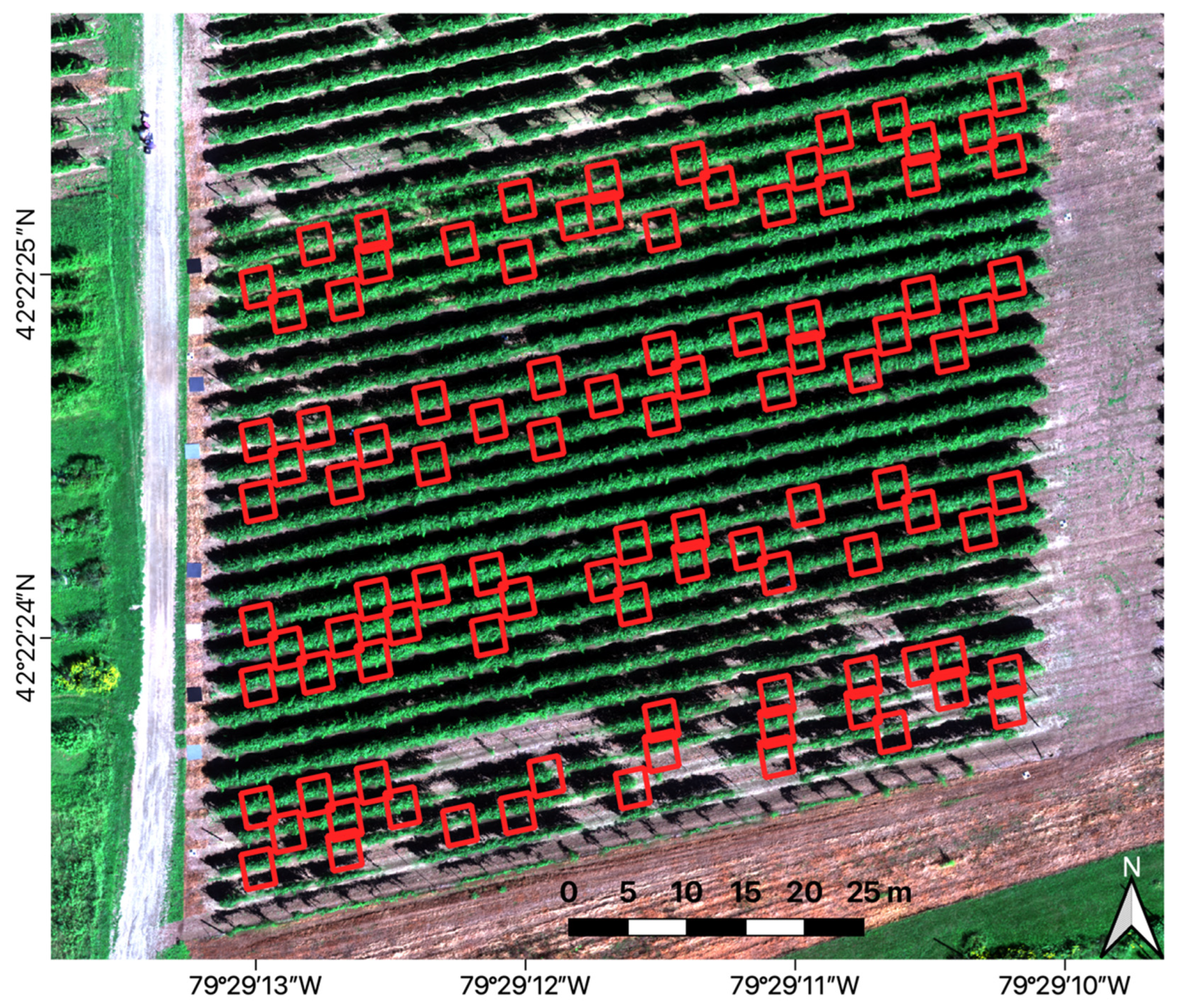
Figure 1. MicaSense Rededge-M 5-band reference imagery (RGB channels shown; see Section 2.2) of the 1-acre Concord grapevine vineyard block located at CLEREL in Portland, NY, USA. The imagery was taken on 6 September 2021 at 10:55 a.m. EST. The 100 vine sampling locations are marked with red squares (2.5 m × 3.0 m).
Remotesensing 13 04489 g001
Figure 2. Results of each masking of the grapevine canopy steps, including the threshold masks of multiple vegetation indices, a spectral angle mapper canopy classification mask, and a morphological erosion of the multiplied masks. For the VNIR imagery, the NDVI and EGI were used, and for SWIR, the NDNI was used for the vegetation mask thresholds (NDVI > 0.812, EGI > 0.0613, and NDNI > 0.175, respectively). In each case, the threshold value was quantitatively determined from a vegetation index pixel histogram. The final masks were used to extract the mean canopy spectra of each grapevine in the sample.
Remotesensing 13 04489 g002
Figure 3. Average grapevine spectrum with the optimal wavelengths for nitrogen content prediction found using the ensemble (5 orange circles) and PLSR (10 magenta triangles) feature selection methods. The PLSR points are plotted on a spectrum shifted upward to differentiate between the wavelengths selected by the two methods. The location of the MicaSense RedEdge multispectral sensor blue, green, red, red-edge (brown), and near-infrared (gray) bands are noted in the VNIR for the context of a typical multispectral camera used in precision agriculture.
Remotesensing 13 04489 g003
Figure 4. Frequency of the selected wavelengths from all the nutrient ensemble (orange hatch) and PLSR (magenta) models. An average grapevine spectrum is shown in green for interpretation of the relevant spectral regions. The location of the MicaSense blue, green, red, red-edge (brown), and near-infrared (gray) bands are noted in the VNIR for context.
Remotesensing 13 04489 g004
Figure 5. Ratio of the mean spectra from the 10-lowest and 10-highest N-content grapevines. The green ratio spectrum is from the UAS imagery, and the blue (upper) is from the SVC handheld leaf clip spectra obtained from two sample leaves per vine. The vertical lines mark the locations of wavelengths selected from the UAS data for the ensemble (purple solid) and PLSR (orange dashed) methods.
Remotesensing 13 04489 g005
Figure 6. Correlations between individual nutrients in the grapevine leaf samples are shown as a heatmap, with values for Pearson’s correlation, R. There are two primary groups of mutually correlated nutrients: N–P–K–B and Ca–Mg.
Remotesensing 13 04489 g006
Table 1. Grapevine leaf nutrient LOOCV, adjusted R2, and RMSE for the ensemble and PLSR methods.
Method:EnsemblePLSR
NutrientIMT a# W b R 2 RMSE   c # W b R 2 RMSE   c
N (%)2750.440.17100.450.17
P (%)2670.340.0290.510.02
K (%)2450.260.13100.420.12
Ca (%)2590.330.1970.380.18
Mg (%)2670.230.05100.270.04
B (mg/kg)2580.463.08100.463.08
a Number of wavelengths remaining after IMT—initial multicollinearity threshold. b #W—number of selected wavelengths. c Note: The RMSE units differ for macro and micronutrients; see the leftmost Nutrient column.
Table 2. Selected wavelengths for nitrogen and the known nearby absorption features.
Selected (nm)MethodAbsorption (nm)ChemicalBehavior a
--430Chlorophyll aElectron transition
--460Chlorophyll bElectron transition
526Ensemble---
574PLSR---
606Both---
641Both640Chlorophyll bElectron transition
677PLSR660Chlorophyll aElectron transition
958PLSR970WaterO-H bend, 1st overtone
1168Both---
1494Both1510Protein, nitrogenN-H stretch, 1st overtone
2030PLSR---
2058PLSR2060Protein, nitrogenN=H bend, 2nd overtone/N=H bend/N-H stretch
2173PLSR2180Protein, nitrogenN-H bend, 2nd overtone/C-H stretch/C-O stretch/C=O stretch/C-N stretch
a Absorption features related to foliar chemical concentrations identified by Curran [32].
Publisher’s Note: MDPI stays neutral with regard to jurisdictional claims in published maps and institutional affiliations.