Retrieval of Firn Thickness by Means of Polarisation Phase Differences in L-Band SAR Data

Abstract

The knowledge of glacier zones’ extent and their temporal variations is fundamental for the retrieval of surface mass balance of glaciers and ice sheets. In this context, a key parameter is the firn line (FL), the lower boundary of the percolation zone, whose location is an indicator of time-integrated mass balance changes. Several approaches have been developed in the last decades to map the FL by means of Synthetic Aperture Radar (SAR) imagery, mainly exploiting backscatter intensities and their seasonal variation. In this paper, an alternative approach is proposed, based on co-polarisation phase differences (CPDs). In particular, CPDs are interpreted as the result of propagation through anisotropic firn layers and are, therefore, proposed as an indicator of the presence of firn. A model is employed to demonstrate the link between CPDs and firn depth, indicating the potential of polarimetric SAR to improve firn characterization beyond spatial extent and FL detection. The proposed approach is demonstrated on L-band airborne data, acquired on 21 May 2015 by the F-SAR sensor of DLR in West Greenland during the ARCTIC15 campaign, and validated with in-situ information available from other studies.

1. Introduction

The potential of SAR measurements to map glacier zones has been demonstrated in several studies in the context of single-polarimetric backscattering observations [1,2,3], as well as multi-polarisation and multi-frequency Synthetic Aperture Radar (SAR) data [4]. In [5,6], the detection of the firn line (FL) using C- and L-band backscattering coefficients has been addressed. One of the first algorithms for deriving firn maps was presented in [7], where the FL retreat on the Svartisen ice cap was demonstrated over a seven-year period using C-band winter backscatter measurements. A similar method was used in [8] to monitor the FL retreat on the Blamannsisen ice cap between 1992 and 2010. A common limitation in both studies is the difficulty to detect thin firn layers close to the FL. In fact, backscatter from firn is typically associated to the presence of refrozen melt features, such as ice layers and lenses. Thin firn layers contain a smaller amount of such inclusions compared to thicker layers and, therefore, are associated to significantly lower backscattering. This makes the detection of the transition from thin firn to bare or snow-covered ice difficult. An attempt to identify the thin firn boundary on the Qinghai-Tibetan Plateau using summer C-band backscattering images was presented in [9]. In [10], a technique based on statistical modelling of polarimetric covariance matrices was developed to detect the FL using multi-temporal dual-polarisation C-band data.

An important recent contribution was the demonstration of a birefringent behaviour of firn (and snow) induced by its anisotropic microstructure [11,12]. This is caused by the elongation of the grains resulting from temperature gradient mechanisms [13,14]. The model presented in [11] describes co-polarisation phase differences (CPDs), i.e., the phase difference between the HH and VV polarimetric channels, as the result of propagation effects through a firn layer. The model was employed in [15] to demonstrate the retrieval of firn (layer) thickness in the accumulation zone of the Austfonna ice cap from L-band CPDs. Similar anisotropic propagation effects were observed in sea ice [16] and attributed to the presence of oriented spheroidal brine inclusions, which cause birefringence [17]. A refined version of the model in [11], accounting for different vertical distributions of scatterers in the firn volume, was proposed in [18].

In this communication, the potential to use CPD, by means of the model introduced in [18], to estimate the firn thickness on a 200-km long swath acquired over the K-transect, in West Greenland, covering the transition from the ablation to the lower percolation (firn) zone of the ice sheet is discussed. For this, L-band polarimetric data included in the multi-frequency dataset used in [18] are employed. The objective is to demonstrate the potential to make a step forward with the retrieval of firn thickness, beyond the estimation of the FL location addressed in [18]. The employed model is described in Section 2. Section 3 introduces the study area and the SAR data. Section 4 presents the inversion approach as well as the results of the firn thickness estimation and their discussion. Finally, conclusions are drawn in Section 5.

2. CPD Model for Firn Mapping

The CPD model proposed in [18] allows to describe the propagation of electro-magnetic waves through birefringent media with slightly different velocities at different polarisations, introducing phase differences between the polarimetric channels. Consistently to [15,18], the CPD is defined as:

$$CPD={\phi }_{HH}-{\phi }_{VV}$$

(1)

where ${\phi }_{HH}$ and ${\phi }_{VV}$ are the phase terms of the signal measured in the HH and VV channel of a polarimetric SAR sensor, respectively.

Due to its anisotropic microstructure, firn becomes birefringent [13]. In [15,18], firn is modelled as a granular non-scattering medium composed of a two-phase mixture of air and spheroidal ice grains, with the latter being assumed uniformly distributed, equally shaped and oriented.

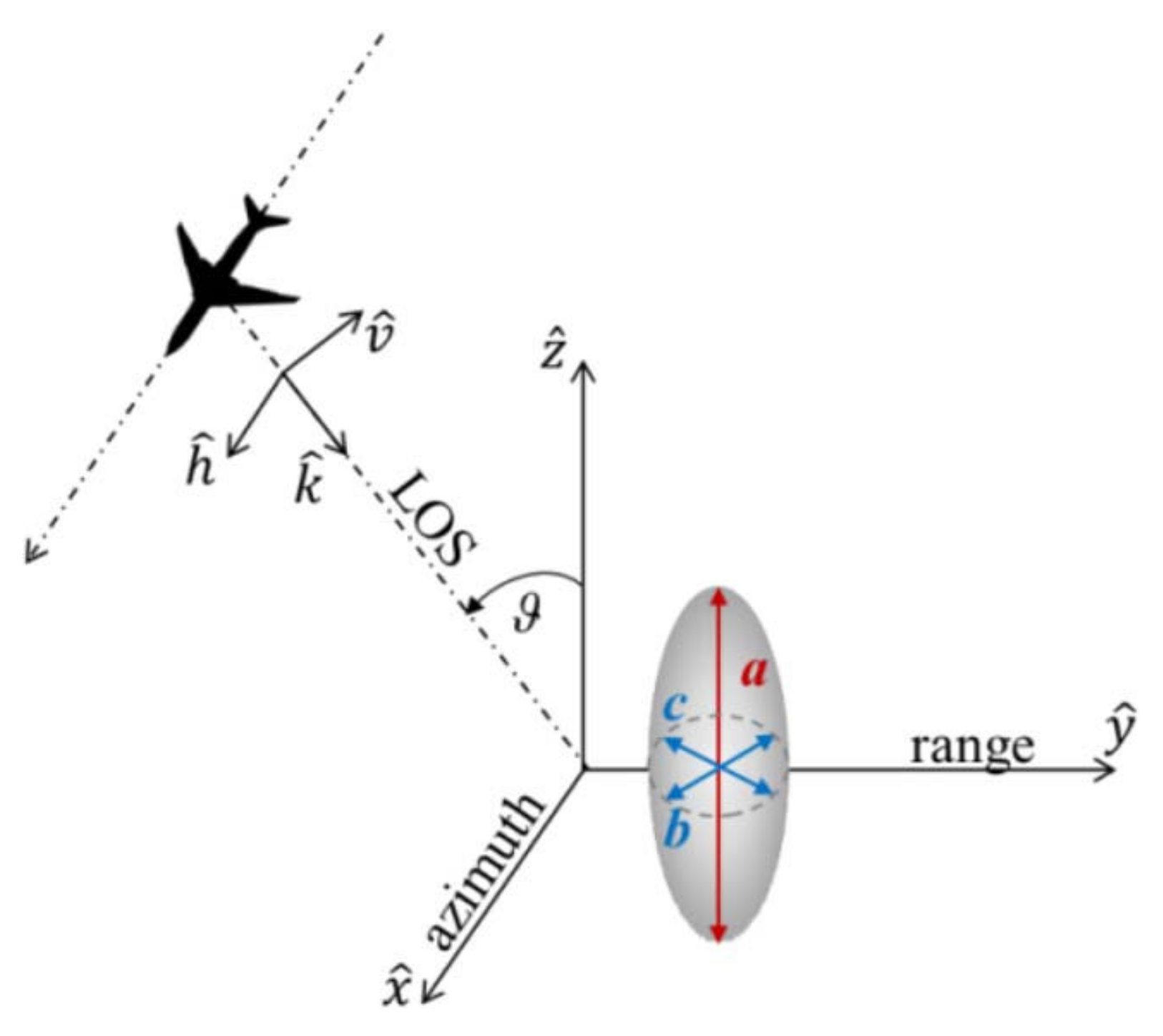
The permittivity components of the material, ${\epsilon }_{firn,x}$, ${\epsilon }_{firn,y}$ and ${\epsilon }_{firn,z}$, in the $\left(\widehat{x},\widehat{y},\widehat{z}\right)$ orthonormal reference system (see Figure 1) can be written as [18]:

$${\epsilon }_{firn,x,y,z}={\epsilon }_{air}+\mu {\epsilon }_{air}\frac{{\epsilon }_{ice}-{\epsilon }_{air}}{{\epsilon }_{air}+\left(1-\mu \right) N_{x,y,z} \left({\epsilon }_{ice}-{\epsilon }_{air}\right)}$$

(2)

where ${\epsilon }_{air}$ and ${\epsilon }_{ice}$ are the air and ice permittivity, respectively, while $\mu$ is the ice volume fraction, directly linked to the density of the firn layer (${\rho }_{firn}=\mu {\rho }_{ice}$, with ${\rho }_{ice}=0.917$ g/cm³). The dielectric birefringence results from the structural anisotropy, which is accounted for in Equation (2) by the depolarisation factors $N_{x,y,z}$ determined by the ice grain shape. The latter is described by means of the grain shape factor $S_p=a/b$, defined as the ratio of the vertical to the horizontal axis of the spheroidal particles used to model the grains.

The effective permittivity components of Equation (2) need to be projected onto the $\widehat{h}$ and $\widehat{v}$ polarisations direction in order to describe the propagation of the H and V polarized pulses [18]:

$${\epsilon }_{firn,h}={\epsilon }_{firn,x}, {\epsilon }_{firn,v}={\epsilon }_{firn,y}{\cos }^2{\vartheta }_r+{\epsilon }_{firn,z}{\sin }^2{\vartheta }_r$$

(3)

where ${\vartheta }_r$ is the refracted radar incidence angle. Finally, the CPD measured by the sensor is proportional to the two-way propagation path of the SAR signal through the anisotropic firn layer and, therefore, proportional to the thickness l of the firn layer sensed by the radar [18]:

$$CPD=arg\left(\underset{0}{\overset{l}{{\displaystyle \int }}}\sigma \left(z\right) e^{-2j\frac{2\pi }{\lambda }\sqrt{{\epsilon }_{firn,h}}\frac{z}{\cos {\vartheta }_r}}{\left(e^{-2j\frac{2\pi }{\lambda }\sqrt{{\epsilon }_{firn,v}}\frac{z}{\cos {\vartheta }_r}}\right)}^{*}dz\right).$$

(4)

λ is the radar wavelength and $\sigma \left(z\right)$ the vertical backscattering distribution (generated by ice lenses, pipes, layers) in the firn. In the simplest case, $\sigma \left(z\right)$ is approximated by an exponential function corresponding to a volume of scatterers with a constant signal extinction coefficient $k_e$:

$$\sigma \left(z\right)=e^{-\frac{2k_e}{\cos {\vartheta }_r}z}$$

(5)

where $k_e=\cos {\vartheta }_r/l$. Although this is a very simple approximation, it proved to be appropriate at L-band for the lower percolation zone of Greenland [19] addressed in this study.

According to Equation (4), the vertical elongation of the ice grains in a firn layer can exclusively interpret positive CPD values [18]. These can, therefore, be used as indicators of the presence of firn, with the CPD being proportional to the layer thickness: larger phase differences are associated to thicker layers and vice versa. However, it must be reminded that (positive) CPDs can also be introduced by scattering processes, as for example multiple-reflections. Such scattering contributions can usually be recognized by means of their spatial characteristics, as they occur spatially isolated or in distinctive patterns (e.g., crevasses). A more critical CDP contribution is the one from metamorphic snow layers that have a similar birefringent behaviour as firn [20]. Metamorphic snow also underwent temperature gradient metamorphism, which forms vertically elongated grains [20] and leads to positive CPDs. This makes it challenging to distinguish a thin layer of firn from metamorphic snow. Finally, a possible CPD term induced by the dielectric properties and shape of the icy scatterers present in the firn volume [21] is expected to be negligible (in the order of 4° for any incidence angle and particle shape, at the frequency of interest) as discussed in [18].

Model Sensitivity

According to Equation (4), the CPD induced by a layer of anisotropic firn depends on two sensor parameters—the wavelength $\lambda$ and incidence angle $\vartheta$—and on the three firn properties: density ${\rho }_{firn}$, thickness $l$ and grain shape factor $S_p$. The behaviour of the model with respect to such parameters is assessed in the following.

The CPD increases with decreasing wavelength, indicating that differential propagation effects become more significant at higher frequencies. According to Equation (4), for a reference firn layer of $l=1 \mathrm{m}$ with $S_p=1.3$ and ${\rho }_{firn}=0.6 \mathrm{g}/\mathrm{c}{\mathrm{m}}^3$, at an incidence angle of $\vartheta =$ 30°, the CPD reaches 28° at X-band ($\lambda$ = 0.03 m), 16° at C-band ($\lambda =$ 0.05 m) and 4° at L-band ($\lambda =$ 0.22 m).

The effect of the angle of incidence is significant. Since firn anisotropy is only vertical, propagation effects are absent for $\vartheta =$ 0°, when the line-of-sight (LOS) is aligned to the nadir and both $\widehat{h}$ and $\widehat{v}$ polarisations lie in the horizontal plane, aligned to the two equal axes of the grains (see Figure 1). By increasing $\vartheta$, the $\widehat{v}$ axis rotates toward the vertical direction ($\widehat{z}$), parallel to the anisotropy direction, while the $\widehat{h}$ polarisation remains parallel to the horizontal plane. This maximizes the dielectric anisotropy between the two polarisations and, in turn, the induced propagation effects. Moreover, the propagation path through the anisotropic layer increases with the incidence angle, according to $z/\cos \vartheta$, further contributing to the rise of the CPD. For a firn layer with $l=1 \mathrm{m}$, $S_p=1.3,$ and ${\rho }_{firn}=0.6 \mathrm{g}/\mathrm{c}{\mathrm{m}}^3$, the L-band CPD increases from 2° to for 15° when $\vartheta$ increases from 20° to 60° across range.

Concerning the grain shape$,$ spherical grains ($S_p=1$) do not cause anisotropy and, therefore, lead to zero CPD. The latter increases with the vertical elongation of the grains ($S_p>1$) causing positive CPDs values, while oblate grains ($S_p<1$) induce negative CPDs as in the case of fresh snow [12,20]. According to Equation (4), for a firn layer with $l=$ 1 m and ${\rho }_{firn}=0.6 \mathrm{g}/\mathrm{c}{\mathrm{m}}^3$ the L-band CPD ranges, at an incidence angle $\vartheta =$ 30°, from slightly less than 1° to 5° for $S_p$ values between 1.05 and 1.4 associated, according to Equation (2), to a dielectric anisotropy ($\Delta \epsilon ={\epsilon }_z-{\epsilon }_{x,y}$) ranging from 0.015 to 0.085, in agreement with the values reported for Greenland [14] and Antarctica [22]. Overall, a $15\%$ inaccuracy in the knowledge of $S_p$ leads to a $44\%$ uncertainty in the L-band CPD. The accurate knowledge of firn anisotropy is, therefore, critical for a reliable inversion of the model to estimate thickness.

Finally, the behaviour of the CPD model with respect to firn density is not monotonic, in contrast to the case of particle shape. At lower densities (${\rho }_{firn}<0.45 \mathrm{g}/\mathrm{c}{\mathrm{m}}^3$), the CPD increases with density as the volume fraction of the (elongated) ice grains increases, inducing a stronger dielectric anisotropy. At higher densities (${\rho }_{firn}>0.45 \mathrm{g}/\mathrm{c}{\mathrm{m}}^3$), the effect of the grain shape ($S_p$) decreases more and more as all air pores between the particles (grains) gradually close, and the induced CPD reduces accordingly. For a firn layer with $l=$ 1 m and $S_p=$ 1.3, the induced L-band CPD at $\vartheta =$ 30° decreases from approximately 5° to 2° for firn density increasing from $0.5 \mathrm{g}/\mathrm{c}{\mathrm{m}}^3$ to $0.8 \mathrm{g}/\mathrm{c}{\mathrm{m}}^3$. On average, a 15% inaccuracy in the knowledge of ${\rho }_{firn}$ leads to a 14% uncertainty in the L-band CPD, indicating a smaller impact than for the particle shape.

3. Test Site and Experimental SAR Data

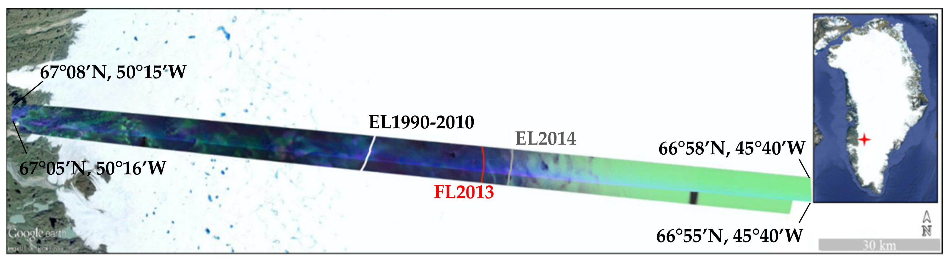
The dataset employed to test the firn thickness retrieval approach was acquired in Greenland by the airborne F-SAR sensor of DLR in the frame of the ARCTIC15 campaign, on 21 May 2015 [23]. An approximately 200 km long (and 5 km wide) swath was imaged at multiple frequencies, including L-band, in fully polarimetric mode, overflying the K-transect (67°04′ N, 49°23′ W) along two opposite flight directions (headings): the “ascending” swath starts at the ice margin and crosses the ablation and the superimposed ice (SI) zones in W-E direction, up to the lower percolation zone (approximately 2100 m a.s.l.); the “descending” swath was flown in the opposite direction (heading). It is worth to notice that the two swaths are slightly shifted with respect to each other and overlap only partially in the range direction (see Figure 2). The SLC (single-look complex) data have been acquired with a spatial resolution of 2.0 m in (slant-) range and 0.5 m in azimuth. The incidence angle varies across the swath from 25° (in near-range) to 65° (in far-range). During the whole campaign, the air temperature was steadily below 0 °C, so that dry snow and ice conditions were preserved. Furthermore, no precipitation event is reported by the ground team on the acquisition day and in the days before.

With respect to the imaged swaths, the ablation zone roughly extends from the coast (left side of Figure 2) up to the long-term (average over the 1990–2010 period) equilibrium line (EL). Although 2014 is the reference mass balance year in this study, the 2014 EL is not used for the delineation of the ablation zone as it was shifted to exceptionally high altitudes (compared to its location in the previous and following years) [24]. Instead, a more representative EL location for the period between 1990 and 2010 is used at an altitude of about 1500 m a.s.l. The lack of information about the FL location in 2014 allows only an approximate location of the SI zone, which is assumed to extend from the long-term EL up to the FL2013 (1680 m a.s.l.). Finally, the percolation zone, characterized by the presence of firn, is found above the FL2013, on the right side of Figure 2. The area between the FL2013 and 1850 m a.s.l., slightly above the EL2014, is considered to be part of the transition from the percolation to the SI zone, where the subsurface consists of a mixture of firn and ice layers [25].

4. Firn Thickness Inversion

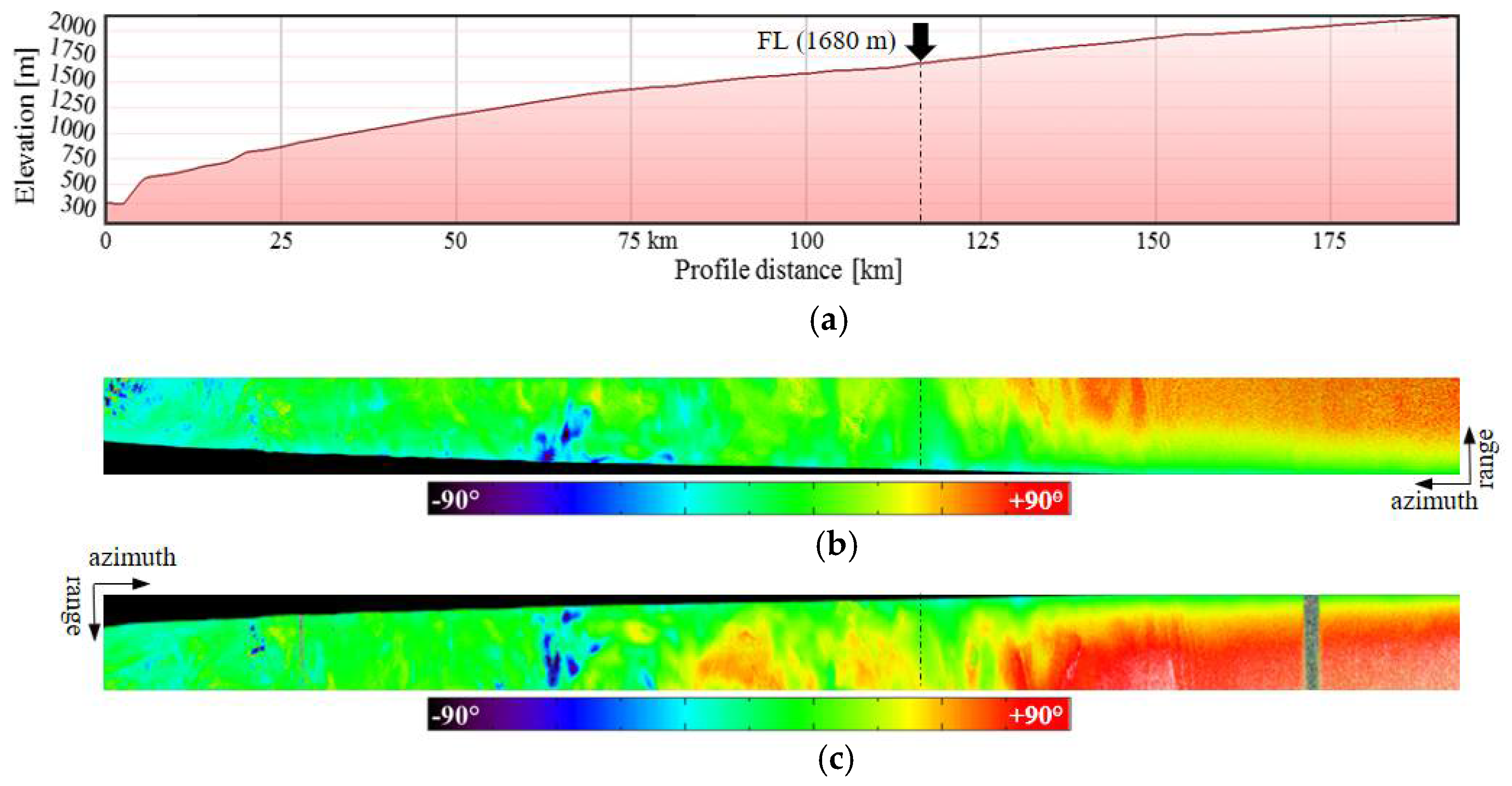
The L-band CPD maps for both headings are depicted in Figure 3b,c along with the elevation profile of the transect (Figure 3a). The two maps are fairly similar, except for the trend in the range direction due to the opposite look directions. CPD values are positive, with few exceptions in localized areas of the ablation zone. A qualitative interpretation of the CPDs across the different zones and of their incidence angle dependency can be found in [18]. Here, the potential of using the CPDs for firn thickness estimation by inverting Equation (4) is discussed. As mentioned in Section 2, the anisotropic microstructure of firn can only cause positive CPD values. Therefore, negative values are assumed to indicate the absence of firn and the corresponding firn thickness is set to 0 m. In Equation (4), $\lambda =$ 0.22 m and the incidence angle variation across range with $\vartheta \in \left[25°, 65°\right]$ are known; ${\epsilon }_{firn,h}$ and ${\epsilon }_{firn,v}$ are computed according to Equation (3), where the bulk firn density is fixed to ${\rho }_{firn}=$ 0.6 g/cm³ according to the ice core analysis in [25], and the (grain) particle shape to $S_p=$ 1.3, using the values measured in the dry snow zone of Greenland [13] since no measurements are available from the study area. Setting $S_p$ to a constant value might be a strong assumption as firn anisotropy (i.e., grain shape) depends on several factors, such as accumulation rate and subsurface temperature gradients, which vary significantly across the ice sheet. However, the assumed $S_p$ value corresponds to a dielectric anisotropy of around 0.05, which is in the range of values reported also for other locations of Greenland [14] and Antarctica [22]. The parameters used in Equation (4) are listed in

Table 1. List of input parameters for the model-based inversion of firn thickness.

Radar Parameters	Firn Parameters
$\lambda =0.22$ [m]	${\rho }_{firn}=0.6$ [g/cm3]
$\vartheta =25-65$ [deg]	$S_p=1.3$

.

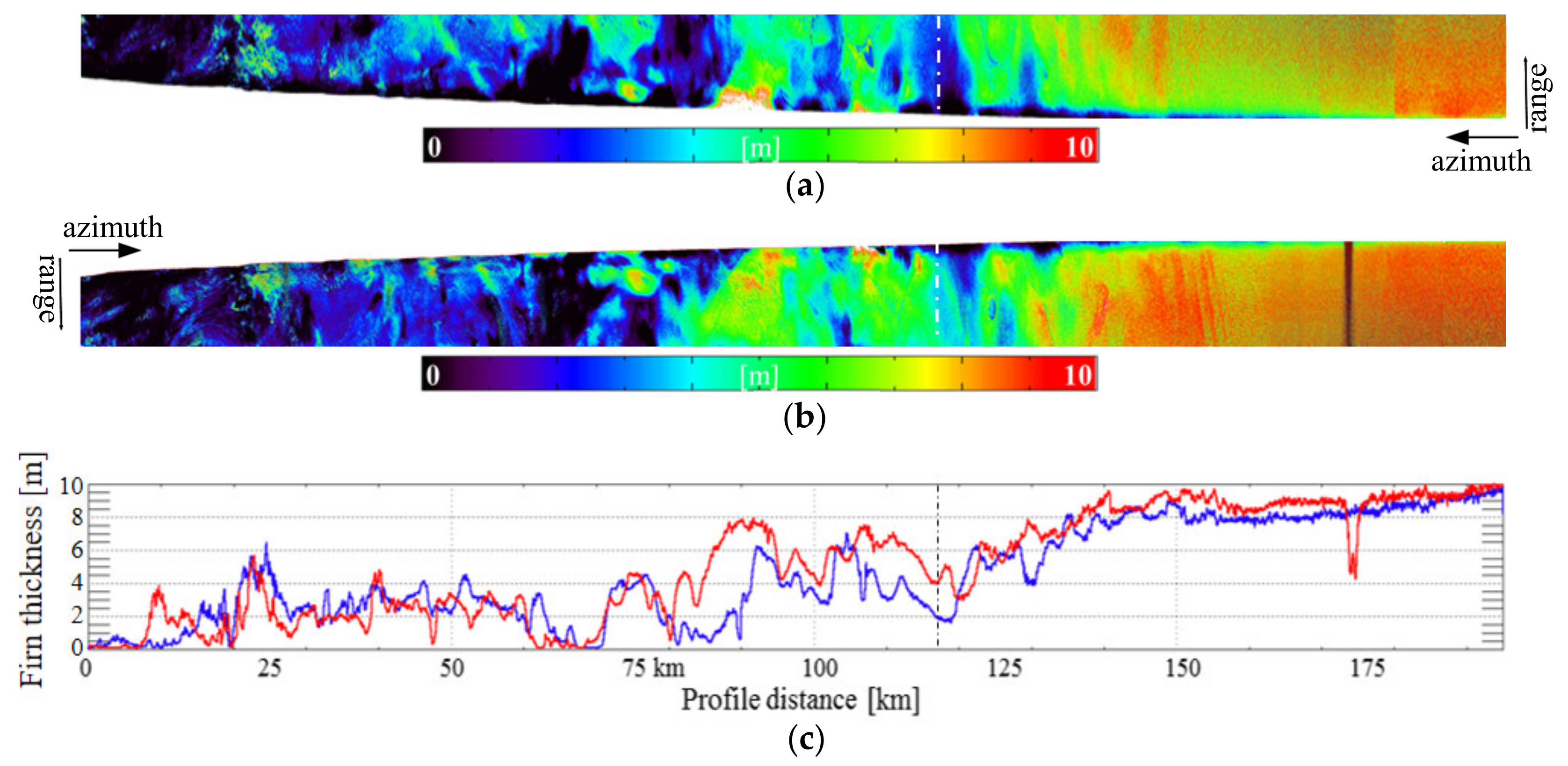
By fixing the bulk density and the grain shape, the firn thickness l is the only unknown parameter in Equation (4) and can be inverted from the measured CPDs. The firn thickness maps obtained for the two headings are shown in Figure 4. Despite that the two swaths are shifted in range, a similar overall pattern can be observed for the retrieved values. In particular, the strong gradient of CPD observed in the range direction over the percolation zone (see Figure 3) is no more present in the thickness maps, except for the very near range, pointing out the ability of the model to correctly account for the large incidence angle variation. To better assess the variation of the obtained firn thickness along the transect, azimuth profiles have been extracted (see Figure 4c) by averaging over 500 range samples (corresponding to a width of approximately 600 m) at the middle range of each heading (corresponding to an average incidence angle of 50°).

Both estimated maps and their corresponding azimuth profiles indicate the presence of a fairly homogeneous firn layer, starting at 140 km profile distance (approximately 1900 m a.s.l.) with thickness values from 8 m to 10 m despite the expectation of a continuously increasing firn thickness with increasing (terrain) altitude. This saturation can be attributed to the fact that the L-band signal only penetrates several meters into the subsurface of the lower percolation zone [19]. At lower elevations, a gradual decrease of firn thickness is obtained, down to approximately 1680 m a.s.l. (at around 118 km distance) where the firn thickness reaches a local minimum for both headings (see Figure 4c). This is in accordance with the gradual replacement of firn with a thick layer of superimposed ice reported in [25] for the same altitude range. In addition, the location of the minimum thickness matches well with the known FL position while the local minimum of 1.9 m and 3.9 m for the “ascending” and “descending” heading, respectively, are still larger than the expected firn disappearance. Finally, the discrepancies between the two profiles in this altitude range are due to the fact that they refer to different locations, as the swaths associated to the two headings are displaced from each other.

At lower elevations, the estimated firn thickness is generally lower and follows the irregular patterns of the CPDs. However, the interpretation of the results below the FL requires the consideration of several factors. In general, the retrieval of firn thickness values larger than 0 is in contradiction with the expected absence of the firn itself. Firstly, with the SAR data acquired in May, at the end of the accumulation season, it is reasonable to expect the presence of a metamorphic snow layer accumulated at the ice surface during the winter months. Such a layer induces a positive CPD term [20], which biases the estimated firn thickness. Snow accumulation data from [26] report typical snow heights varying from 30 cm at around 500 m a.s.l. to 1 m at 1850 m a.s.l. over the K-Transect. Such a snow layer is able to explain, at least partially, the values below the FL.

Finally, localized features showing higher thickness values correspond to crevasse fields as visible between 70 km and 110 km distance in the azimuth profiles in Figure 4c. Interestingly, this portion of the transect also shows larger discrepancies between the two profiles. As mentioned above, the two opposite swaths are displaced in range and, therefore, localized and oriented features, such as crevasse fields, contribute differently to the corresponding azimuth profiles. Crevasses can be avoided by introducing a pre-processing step aiming at detecting and excluding them from the inversion algorithm. Their detection can be performed on the basis of their distinct spatial patterns and/or their polarimetric signatures.

Model Limitations and Possible Improvements

As discussed in Section 2, the model in Equation (4) relies on some simplifying assumptions which inevitably impact the validity of the inversion results. For instance, firn properties, such as density and anisotropy, are assumed to be spatially constant while they are known to vary both horizontally and with depth. Any inaccuracy of the assumed values directly translates into a bias on the estimated firn thickness. A 10% error on the density value leads to an average 10% bias on the estimated thickness for incidence angles between 30° and 50°. A 10% error on the $S_p$ value translates into an average 35% bias on firn thickness. Given the difficulties in obtaining extensive and accurate reference values for both parameters, further effort is required towards a joint retrieval of firn properties exploiting, for instance, independent CPD measurements obtained from multi-angular acquisitions [27].

A further simplification is made when assuming a given vertical backscattering distribution $\sigma \left(z\right)$ across the whole scene. In this sense, vertical backscattering profiles derived from interferometric or tomographic SAR acquisitions can provide a good starting point for considering a space-varying $\sigma \left(z\right)$ [28] at the cost of an increased observation space. In addition, the measured CPDs are entirely attributed to the propagation through the firn layer, considering possible additional contributions from other sources to be negligible. This becomes problematic in the presence of a multi-layer scenario where firn underlies a snow layer. For instance, a fresh snow layer is expected to generate a negative CPD term [12], typically in the order of a few degrees at L-band, which leads to an underestimation of the firn thickness.

5. Conclusions

In this study, the potential of L-band CPDs for the retrieval of firn thickness has been discussed. For this, a model-based inversion of CPDs has been performed using airborne SAR data acquired along a 200-km long transect in West Greenland covering the transition from the ablation to the percolation zone of the ice sheet. The results compare well to the findings of shallow ice cores and GPR measurements published in other studies, even though these allow only a qualitative validation. A quantitative assessment of the proposed approach would require distributed measurements of firn thickness, density, and anisotropy, which are difficult to perform. Even if the performance of the estimation may be affected by the simplifying assumptions in the model inversion, the fact that it is based on a physical model provides a direct link to geophysical parameters of interest and contributes uniquely to the characterization of the subsurface scattering structure in the percolation zone. Furthermore, the approach is based on a single SAR acquisition, which represents a clear advantage over existing SAR-based firn mapping methods that typically require multiple acquisitions to produce binary 2D firn/non-firn maps.

An extension of the inversion scheme to multiple CPD measurements could improve the results and increase the potential of the method: multi-angle measurements, for example, may allow a joint inversion of firn thickness, density, and anisotropy [27]. At the same time, multi-frequency CPD measurements can potentially resolve the variability of snow and firn properties with depth by exploiting the different penetration of the different frequencies. For instance, the sensitivity of X-band CPD measurements to shallow snow layers might be exploited together with the L-band data to detect fresh snow and compensate the underestimation induced on the retrieved firn thickness values.

Finally, the proposed retrieval scheme can be easily transferred to the case of spaceborne data for its use on a larger scale.