Article

Building Extraction from Remote Sensing Images with Sparse Token Transformers

1
Image Processing Center, School of Astronautics, Beihang University, Beijing 100191, China
2
Beijing Key Laboratory of Digital Media, Beihang University, Beijing 100191, China
3
State Key Laboratory of Virtual Reality Technology and Systems, School of Astronautics, Beihang University, Beijing 100191, China
4
Department of Computational Medicine and Bioinformatics, University of Michigan, Ann Arbor, MI 48109, USA
*
Author to whom correspondence should be addressed.
Remote Sens. 2021, 13(21), 4441; https://doi.org/10.3390/rs13214441
Submission received: 15 September 2021 / Revised: 23 October 2021 / Accepted: 29 October 2021 / Published: 5 November 2021

Abstract

:
Deep learning methods have achieved considerable progress in remote sensing image building extraction. Most building extraction methods are based on Convolutional Neural Networks (CNN). Recently, vision transformers have provided a better perspective for modeling long-range context in images, but usually suffer from high computational complexity and memory usage. In this paper, we explored the potential of using transformers for efficient building extraction. We design an efficient dual-pathway transformer structure that learns the long-term dependency of tokens in both their spatial and channel dimensions and achieves state-of-the-art accuracy on benchmark building extraction datasets. Since single buildings in remote sensing images usually only occupy a very small part of the image pixels, we represent buildings as a set of “sparse” feature vectors in their feature space by introducing a new module called “sparse token sampler”. With such a design, the computational complexity in transformers can be greatly reduced over an order of magnitude. We refer to our method as Sparse Token Transformers (STT). Experiments conducted on the Wuhan University Aerial Building Dataset (WHU) and the Inria Aerial Image Labeling Dataset (INRIA) suggest the effectiveness and efficiency of our method. Compared with some widely used segmentation methods and some state-of-the-art building extraction methods, STT has achieved the best performance with low time cost.

Graphical Abstract

1. Introduction

Building extraction from remote sensing images refers to the automatic process of identifying building and non-building pixels in remote sensing images. Building extraction plays an important role in many applications, such as urban planning [1], population estimation [2,3], economic activities distribution [4], disaster reporting [5], illegal building construction, and so forth. It can also be used as an essential prerequisite for downstream tasks like change detection from remote sensing images [6,7].
In recent years, with the development of the hardware, high-resolution remote sensing image data have exploded. Automatic building extraction has attracted increasing attention in both academia and industry. Although the recent advancement of deep convolutional neural networks has greatly promoted the research in this area [2,3,8,9,10,11,12], there are still many challenges. For example, optical remote sensing images are often affected by illumination changes and clouds [2,13,14,15,16,17]. Effective feature representation capability is thus much needed to gain robustness in different time and occlusion conditions. Additionally, building instances may exhibit significantly variant appearances in colors, sizes, and shapes. It is usually difficult to properly extract complete building boundaries from the complex background.
In the past year, transformers have quickly become a research hotspot in the computer vision field. Transformers were first proposed and are widely used in natural language processing (NLP) to model sequence-to-sequence tasks [18]. Then, plenty of methods attempt to adapt transformers to a number of computer vision tasks, and have matched or even exceeded the state-of-the-art performance. In the building extraction task, the transformer-based model may be a potential choice because of its strong feature representation capability, global receptive field, and the capability of modeling long-range dependencies between pixels. However, when dealing with high-resolution image data, transformers are usually computation-inefficient and entail high memory usage [19,20,21,22]. This greatly limits its usability in remote sensing image analysis tasks since both the volume and resolution of high-resolution remote sensing image data have recently been growing exponentially.
In this paper, we propose an efficient method for building extraction based on transformers. Our method has less computational overhead and memory consumption, and is scalable in both spatial and channel dimensions. Our model can be quickly trained, tested, and used by a conventional GPU, and can achieve state-of-the-art accuracy on benchmark datasets. In our method, we represent buildings as a set of “sparse” feature vectors in their feature space, and introduce a new transformer module called the “sparse token sampler” to adaptively select those most effective tokens from the input image. Our motivation is that, since single buildings in remote sensing images usually only occupy a very small part of the image pixels, the image tokens can be reduced to a set of sparsely located vectors (viewed as visual words or tokens). We also design a dual-pathway transformer architecture that learns the long-term dependency of tokens in both their spatial and channel dimensions. Thus, long-range dependencies can be discovered between sparse tokens rather than dense pixel-wise features or image patches as in previous efforts [23,24,25,26,27]. As a result of drastically decreasing the sequence length of the transformer input, our design can achieve high efficiency. Section 2.6 contains a comprehensive introduction and analysis. We apply the transformers on a relatively high-resolution feature map to keep local details of the output, meanwhile, the global context can be well modeled. We refer to our method as Sparse Token Transformers (STT). Figure 1 shows the speed–accuracy trade-off and some comparable results between the proposed method and other state-of-the-art segmentation methods.

1.1. Traditional Method for Building Extraction

Traditional methods are mostly based on the hand-craft features under the guidance of the prior knowledge and certain application situations, and then take the classifying, clustering or segmenting algorithms to achieve building discrimination. Sirmacek et al. [28] present an approach for building detection using multi cues including invariant color, edge, and shadow information. Zhang et al. [29] and Zhong et al. [30] utilize spectrum features to improve the building extraction accuracy. Building edges [31,32], building roof texture information [29,33,34], and building shadows [28,35,36] are also explored to achieve the potential of the building extraction task. The methods mentioned often aim at specific tasks with specific datasets by the empirically designed features, which take the buildings’ shape, color, edge, surrounding environment, texture, height, shadow, and so forth, into account. They are under too many restrictions and are far from being termed as a universal building extraction method for practical application. Besides, their performance is limited due to the self-selected features and the self-designed parameters.

1.2. CNN-Based Method for Building Extraction

In recent years, the progress of technology and hardware has promoted the development of deep learning. In deep learning, building extraction can be essentially viewed as a pixel-wise binary image labeling problem. In this problem, Convolutional Neural Network (CNN) and its variants have long been favored by researchers due to its powerful image feature representation ability. Once the most widely used network for low-level pixel-wise labeling tasks was the Fully Convolutional Networks (FCN) [37]. FCN can adapt well to inputting images of an arbitrary size and can be trained in an end-to-end learning manner. Later on, many building extraction methods gradually improve the segmentation results by modifying the structure of FCN [3,4,38,39,40]. SRI-Net [38] designs a spatial residual inception module and integrates the module into the FCN network to capture multi-level semantic features, which achieves a good performance on the detection of multi-scale buildings.
In FCN based methods, as the network layers are going deeper, the receptive field is gradually enlarged, where the context information is enhanced but the local details are lost. To improve the segmentation of details, skip-connection, multi-scale feature fusion, and atrous convolution operations are typically designed in FCN based labeling models. For example, UNet [41] introduces a contracting path to capture context features, a symmetric expanding path to enable precise local features, and direct links between the encoder layers and the corresponding layers in the decoder. SegNet [42] introduces non-linear upsampling layers in its decoder by using the pooling indices computed in the max-pooling step of the corresponding encoder. The DeepLab series tackles the multi-scale problem and achieves a large receptive field with the atrous convolution layer and the atrous spatial pyramid pooling (ASPP) operation [43,44,45]. These methods are typical in the natural image segmentation task and receive an effective performance.
Recently, there are many papers to improve the building extraction performance by focusing on network architecture designing. Structures such as deep and shallow feature fusion [8,38,46,47,48,49,50,51,52,53,54,55], multiple receptive field [5,12,48,51,54,55,56,57], residual connection [1,11,47,51,52,57,58,59] have been widely used in building extraction. MAP-Net [46] alleviates the scale problem by capturing spatial localization-preserved multi-scale features through a multi-parallel path design. BRRNet [12] introduces a prediction head to extract global context with the atrous convolution of different dilation rates and a residual refinement part to improve the accuracy. ESFNet [56] aims to reduce the computational complexity and memory usage by using separable factorized residual blocks and dilated convolutions. In addition to the multiscale design, attention modules are also frequently used in recent building extraction methods [1,2,46,47,58,60,61,62]. Liu et al. [60] propose a multiscale fusion network for learning multiple building features at various scales. Guo et al. [61] use scene prior to minimize misclassification areas and preserve robustness. DANet [63], a classic attention network in segmentation tasks, proposes two types of self-attention modules in the traditional dilated FCN to capture rich contextual dependencies. DAN-Net [62] employs a spatial attention fusion module to enhance different level features in building extraction.
While these methods have made significant advancements in terms of building extraction, there is still a contradiction between global perception ability and processing efficiency. While increasing the receptive field is beneficial for enhancing the performance of semantic segmentation tasks, the majority of existing approaches achieve this by stacking a large number of convolutional layers, which causes the network to pay greater attention to high-level semantic information. Local features, such as edges, would be difficult to precisely segment. The researchers address the issue by providing a deep and shallow feature fusion strategy that preserves shallow features while improving performance for details. These, however, invariably result in increased computational and memory overhead. Due to the amount and resolution of the data, it is not suitable for remote sensing data processing. Our solution aims to obtain full-image receptive while retaining local information in a low-cost architecture based on transformers.

1.3. Transformer-Based Method

More recently, great efforts have been made in the computer vision community to get rid of traditional convolution layers and apply attention-alone models with transformers to break the fundamental limitation of CNNs. Transformers can learn explicit long-range dependencies, which are particularly suitable for pixel-wise labeling tasks in position-unconstrained remote sensing images. Some promising works on applying transformers in the remote sensing field have recently emerged, including image classification [19], change detection [6], image caption generation [64], hyperspectral image classification [20,65], segmentation [66], and so forth. SETR [27] expands transformers on the natural image segmentation task, which conducts a standard transformer encoder and a convolutional decoder. It views the semantic segmentation as a sequence-to-sequence task. Bazi et al. [19] applied vision transformers to remote sensing scene classification and achieve a good performance. Chen et al. [6] employ an efficient transformer method for remote sensing image change detection and achieve a state-of-the-art performance, compared with other methods.
Despite the recent progress, standard transformers are of high computational complexity and memory usage. DETR [26] presents a hybrid CNN-transformer approach for object detection, treating it as a set prediction problem. However, it takes longer to converge than other approaches based on CNN. Additionally, DETR executes transformer layers on relatively low-resolution feature maps acquired via CNN backbone to maintain efficiency. As a result, it is unsuitable for detecting small objects. Deformable DETR [67] resolves the stalemate by only focusing on a limited set of crucial sampling points around a reference using deformable convolution. With ten fewer training epochs, deformable DETR can outperform DETR (particularly on small objects). In our work, we take advantage of the capability of transformers to capture global dependencies and, at the same time, hope to model the global content efficiently. The primary distinction between our method and the previous one is that we employ a sparse token sampler and a dual-pathway transformer architecture for the building extraction task. Specifically, unlike Deformable DETR, our sparse token sampler samples the sparse key feature vectors explicitly, whereas Deformable DETR predicts the location of the key points via deformable convolution and then acquires the feature vectors via bilinear interpolation. The network training process implicitly learns the placement of crucial points. Second, the STT encoder only considers the key vectors for self-attention, whereas the transformer encoder in Deformable DETR uses the whole feature map as the query set. Additionally, we suggest a dual-way transformer structure for simulating spatial and channel interdependence. Significantly, STT is optimized for building extraction, whereas Deformable DETR is optimized for detection. Thus, in our study, the transformer is utilized to construct global dependencies on relatively shallow feature maps in order to acquire a large receptive field without sacrificing local details, in contrast to Deformable DETR, which relies on high-level semantics for detection. The global context can be efficiently represented in our method using the sparse token sampler and the dual-way transformer. To our knowledge, little study has yet been conducted on these two topics, particularly in building extraction from remote sensing images.

1.4. Contributions

This paper attempts to resolve the aforementioned limitation by adopting a dual-path transformers in an efficient way. The contributions of our work can be summarised as follows:
  • An efficient building extraction method based on transformers is proposed. Instead of progressively extracting large-scope information by stacking convolution layers, we design a spatial and a channel transformer to capture the global context and receive a global receptive field;
  • We introduce a sparse token sampler to generate semantic sparse tokens in the low-resolution feature map. This design significantly improves computation efficiency. Furthermore, it can also be considered as a regularization scheme to achieve a good generalization performance;
  • We evaluate our method on two public benchmark datasets—the Wuhan University Aerial Building Dataset (WHU) and the Inria Aerial Image Labeling Dataset (INRIA). The experiment results show the effectiveness and efficiency of our method. Our method achieves 90.48% Intersection over Union (IoU) on the WHU building datasets, and surpasses many state-of-the-art methods in building extraction. For example, our method is +2.79% higher than DAN-Net and runs 6.4 times faster.

2. Materials and Methods

2.1. An Overview of STT

In our work, we handle the building extraction from the remote sensing images task as a binary classification problem, using a transformer based architecture. Figure 2 shows an overall description of the proposed method. We follow a hybrid CNN-transformer architecture to leverage the advantage of both convolutions and transformers. Our key motivation is that a single building in remote sensing images only occupies a small part of the whole image. Building regions can thus be represented by sparse pixel-wise vectors in the CNN feature maps. Based on this idea, our method learns the potential important spatial positions and channel indices and samples a set of effective tokens based on the spatial and channel probabilistic maps. We regard the top k high-response positions as the representative candidates. The candidate tokens contain sufficient information to mine the long-distance dependencies using self-attention layers.
The proposed method consists of three main components: (i) a sparse token sampler, which generates spare semantic tokens according to the high-response positions in the spatial and channel probabilistic maps; (ii) a transformer encoder, which is designed to explore the potential dependencies between the sparse semantic tokens; (iii) a transformer decoder, which is used to fuse the original features with global contextual information encoded by the transformer encoder, and resume the sparse tokens to the initial resolution. In the following, we will introduce each of them accordingly.

2.2. Sparse Token Sampler

To capture the global contextual information in an efficient manner, we apply the multi-head attention mechanism in the sparse token-based view instead of the whole feature maps. Buildings can be well represented by the sparse tokens, and these selected tokens are used to model the context relationships. The sparse space can be heuristically described by the high-response positions in the spatial and channel probabilistic maps.
To obtain the sparse tokens of a given feature map, we follow the steps below to build the sparse token sampler. Let X * R C * × H × W represent a certain feature map extracted by the CNN feature extractor, where H , W , and C * denote the height, width, and channel of the feature map, respectively. We first reduce the channel dimension of X * from C * to C = C * / 4 with a 1 × 1 convolutional layer, resulting in X . Reducing the channel can help model the context efficiently. Then the modules to generate spatial and channel probabilistic maps are designed to obtain the top k high-response positions or indices. The steps to generate the maps are fully described in Table 1.
We define A i , i { s , c } as the spatial and channel probabilistic maps. The lowercase character s indicates spatial notation and c indicates channel notation. Next, we obtain the top k i high-response positions according to the probabilistic map A i and sample k i feature vectors in the original X as the sparse semantic tokens T i . For spatial sparse tokens T s R k s × C , it is formulated as:
idx s = topk ( A s , k s )
T s = gather ( X , idx s ) ,
where topk ( A s , k s ) denotes the operation of obtaining k s corresponding 2-d coordinate indices of top-k values in the tensor map A s R H × W , and gather ( X , idx s ) means collecting the feature vectors from X R C × H × W along with the specific indices idx s R k s × 2 . For the procedure of sampling channel sparse tokens T c R k c × ( H W ) , it is given by:
idx c = topk ( A c , k c )
T c = gather ( reshape ( X ) , idx c ) .
Here, topk ( A c , k c ) means getting k c 1-d high-response indices from A c R C . reshape ( X ) denotes reshaping the dimensions of X from X R C × H × W to X R C × ( H W ) . Then, we can collect T c R k c × ( H W ) from the reshaped X R C × ( H W ) along with idx c R k c × 1 . In this way, we can obtain the spatial sparse semantic tokens T s and channel sparse semantic tokens T c , respectively.

2.3. Transformer Encoder

We apply a transformer encoder to model the global contextual information between the spatial tokens and channel tokens separately. Here, we first construct the dependency relationships between the positions and the semantic tokens. For spatial position embedding, we initialize an embedding map P s R H × W × C with learnable parameters. Then, the spatial sparse position embedding tokens, P s * R k s × C , can be sampled by idx s in Equation (1). It is defined as:
P s * = gather ( P s , idx s ) .
Similarly, we design a channel index embedding P c R C × ( H W ) . The channel sparse position embedding tokens, P c * R k c × ( H W ) , are gathered by the high-response channel indices idx c in Equation (3). When we obtain P s * and P c * , we can model the long-range dependency relationships by the multi-head self-attention layer. To generate the context-rich spatial sparse token T s * R k s × C , all the needed query Q , key K , value V are computed from T s as:
Q = T s W q K = T s W k V = T s W v ,
where W q , W k , W v R C × d are the learnable parameters of three linear projection layers, d is the dimension to be projected and Q , K , V R k s × d denote the matrices of the projection results. The self-attention procedure for T s * R k s × C can be formulated as:
Att ( Q , K , V ) = σ ( Q P s * T + Q K T d ) V T s * = Γ ( Att ( Q , K , V ) ; W Γ )
where σ is the softmax operation over the channel dimension and Γ ( · ; · ) defines the post processing to refine the contextual features with a linear project layer of learnable parameters W Γ , a dropout layer, a shortcut operation, and a layer normalization function. We set d = C in our model to avoid altering the dimensions of P s * . The computing steps are identical to those above for creating the context-rich channel sparse token T c * R k c × ( H W ) , except that the input is changed to T c .

2.4. Transformer Decoder

After the encoding process, we can use a decoder layer to fuse the original features with the encoded global contextual information. Our decoder is a multi-head cross-attention operation. In the following, we give a detailed description of it.
Given the originally generated feature map X , we first adjust X to fit the input of the decoder by the reshaping operation. We reshape the 3-d tensor X R C × H × W to Z s R ( H W ) × C and Z c R C × ( H W ) . Then, we consider Z i as the query and the encoder output T i * as the key and value. Formally,
Q = Z i W q K = T i * W k V = T i * W v ,
where i { s , c } . By following Equation (7), we can calculate Z i * —the tokens with both global contextual information and local details after the decoding process. Z i * has the same dimensions of Z i . Finally, Z i * is reshaped to the original size of ( C , H , W ) . Note that, since we apply transformers on the relatively shallow feature map X , the decoding output local details (e.g., the contour of the buildings) can be well preserved.

2.5. Prediction Head

At the output end of the transformer decoder, the refined feature map mixing with local and global information has a spatial resolution of H × W , 1 / 16 of the original image in our network. We design a simple upsampling head to recover the full resolution for pixel-level prediction. We first reduce the channel of the features concatenating with Z s * , Z c * and X by a 1 × 1 convolutional layer. The prediction head takes it as the input, and produces a continuous-value prediction map Y R 2 × H × W . The configuration of the prediction head is shown in Table 2.

2.6. Computational Complexity in Transformers

In this subsection, we provide a detailed analysis on the computational complexity of the standard transformer model and the proposed one.
First, we revisit the plain self-attention module in transformers. Given an input feature map I R H × W × C , where H is the height, W is the width, and C is the channel dimension, the plain self-attention operation conducts a query matrix Q R N q × d , a key matrix K R N k × d , and a value matrix V R N v × d , where N is the sequence length, and d is the embedding dimension. In a plain self-attention operation, we always have N k = N v . The computational complexity of the plain self-attention module is O ( N q N k d ) . In the image domain, the query and key elements are usually pixels or image patches. In this case, we have N q = N k = H W / P 2 (P is the patch height). The complexity then becomes O ( H 2 W 2 C / P 4 ) . We can see that the self-attention module suffers from a fourth-power of computational complexity growth with the image height or width.
As a comparison, in our method, we have a spatial transformer encoder, a spatial transformer decoder, a channel transformer encoder, and a channel transformer decoder. The total computational complexity of the transformer part is O ( k s 2 C + H W k s C + k c 2 H W + H W k c C ) . Since we have k s H W and k c C , our method can greatly reduce the computation complexity and only has a quadratic growth of the complexity over the image height or width. Table 3 gives a detailed description of each architecture.

2.7. Network Details

2.7.1. CNN Feature Extractor

We use a lightweight CNN, ResNet18 [69], as our image feature extractor. The ResNet18 is originally designed for classification tasks, which has five stages, each stage reduces the spatial resolution of the image by 1 / 2 . To avoid losing too many spatial details, we only use the first four stages. In this way, given a 512 × 512 image, the shape of the last feature map is 32 × 32 × 256 . We have also experimented with other different CNN extractors such as ResNet50 and VGG [70]. The detailed performances are shown in the experiment section.

2.7.2. Parameter Setting

In our sparse token sampler, we set k s = 64 and k c = 16 to accomplish a trade-off between speed and accuracy based on the dimension 32 × 32 × 256 of the features collected by the CNN backbone indicated in Section 2.7.1 and the controlled experiments described in Section 3.2.2. Additionally, in keeping with our goal, we have considered the distribution and amount of buildings per image while determining the number of sparse tokens. In the transformer encoder and decoder, we set the number of multi-head to k s / 8 for spatial transformers and k c / 4 for channel transformers to learn richer feature representation in different subspaces [6,18,27].

2.7.3. Loss Functions

Given the predicted output Y R 2 × H × W and the corresponding ground truth label map Y ^ , we use the cross-entropy loss to train our networks. We also introduce an auxiliary loss to stabilize the sparse token sampling process. We concatenate the CNN backbone output and the probabilistic maps by ( X A s , X A c ) , and use a DoubleConv layer to produce a low-resolution output map Y D R 2 × H 16 × W 16 directly from the low-level CNN feature maps. The total loss function can be written as follows:
L ( · ) = CE ( Y , Y ^ ) + α · CE ( Y D , Y ^ D )
where CE is the pixel-wise cross-entropy loss function, Y ^ and Y ^ D are the corresponding label maps before and after downsampling. α is a positive number balancing the two loss terms.

2.8. Data

We test our method on two challenge building extraction datasets, WHU [3] and INRIA [71]. Figure 3 gives two samples of them.
WHU: The Wuhan University Building Dataset [3] contains an aerial imagery dataset and satellite imagery datasets. We only experiment on the aerial imagery subset. The subset consists of 8188 non-overlapping RGB images with the size of 512 × 512 pixels. The images from the aerial subset are captured above Christchurch, New Zealand with a spatial resolution of 0.0075 m to 0.3 m. The dataset is divided into a training set (4736 images), a validation set (containing 1036 images), and a test set (2416 images) in [3]. We follow the official settings in our experiments.
INRIA: The Inria Aerial Image Labeling Dataset [71] contains 360 high-resolution (0.3 m) remote sensing images. The images cover dissimilar urban settlements, ranging from densely populated areas (e.g., San Francisco’s financial district) to alpine towns (e.g., Lienz in Austrian Tyrol). Each RGB image has a resolution of 5000 × 5000 pixels. The dataset is divided into a training set and a test set, each with 180 images. Since the authors did not release the label for the test set, we divide the original training set into a training set, a validation set, and a test set with the ratio of 6:2:2. When we train our model, we crop all training images to a set of 512 × 512 image slices with an overlap ratio of 0.9.

3. Results

3.1. Experimental Setup

3.1.1. Evaluation Metrics

We use Intersection over Union (IoU), overall accuracy (OA), and F 1 score to measure the accuracy. These metrics are widely used in the image labeling and building extraction literature [3,9,72] and are defined as follows:
IoU = TP / ( TP + FP + FN ) OA = ( TP + TN ) / ( TP + TN + FP + FN ) F 1 = 2 × Precision × Recall Precision + Recall ,
where Precision = TP / ( TP + FP ) and Recall = TP / ( TP + FN ) . TP, FP, TN, and FN denotes the true positive samples, false positive samples, true negative samples, and false negative samples, respectively.

3.1.2. Training Details

Image augmentation is performed during the training, with random distortion, random expanding, random cropping, random mirroring, and random flipping. We train our networks for 300 epochs. We employ a linear warm-up learning rate schedule to 20 epochs and continue the training with a polynomial decay schedule. We use SGD (stochastic gradient descent) with a momentum optimizer. We set the initial learning rate to 0.01 after warm-up, momentum to 0.9 , and weight decay to 0.0001 . We use the pre-trained model on ImageNet to initialize our CNN feature extractor. The rest of the layers are initialized with a normal distribution. We implement our method by using the Pytorch deep learning framework and train our model with a single NVIDIA Tesla V100 GPU (32G).

3.2. Controlled Experiment

To evaluate the effectiveness of our method, controlled experiments are performed on context composing, sparse token number, position embedding, probabilistic maps and loss functions. We experiment on different versions of our methods. The notation SST ( · ) in the following experiments is described as follows:
  • R 18 ,   R 50 : ResNet18/50 based feature extractor.
  • V 16 : VGG16-based feature extractor.
  • B N : Batch normalization.
  • S 4 ,   S 5 : Different stage output in CNN feature extractor.
  • †: Without auxiliary loss on probabilistic maps.
Unless otherwise stated, all the ablation experiments are performed on SST ( R 18 ,   S 4 ) with default parameter settings and are evaluated using a single scale test protocol on the two datasets mentioned in Section 2.8. We use IoU for the main metric of experiments.

3.2.1. Context Composing

To validate the effectiveness of the spatial transformer and the channel transformer, we conduct an ablation study on different feature fusion strategies under the SST framework, including the single spatial transformer output, the single channel transformer output, and the transformer outputs with the original feature map.
All the spatial and channel transformer modules are employed in a parallel structure, as is shown in Figure 2. Table 4 shows our experimental results. We have the following conclusions: (i) The spatial transformer module and the channel transformer module all work well on the two datasets and outperform ResNet18 ( S 4 ) , which indicates that the context modeling by the sparse tokens is beneficial to the task; (ii) The model with skip connection achieves a considerable improvement by concatenating the original features with the decoder output. This indicates that the residual structure is important not only to CNNs but also to transformers. Features fusing global context information produced by the transformers are of comparative benefit in our method.

3.2.2. Number of Sparse Tokens

We conduct experiments on the number of tokens to give a recommended proposal on the parameter settings in SST. Table 5 shows the comparative results on accuracy. We can see that the number of sparse tokens can greatly affect the speed performance. With the number of sparse tokens increasing, the inference speed (throughput/s) is decreasing sharply. However, after the number of tokens exceeds a certain threshold, such as 64 spatial tokens, we see that the accuracy is saturated and even declining. This also suggests that buildings in an image can be effectively represented by only using a few tokens instead of all of them. Considering both speed and accuracy, we finally set the spatial token’s number to 64 and the channel token’s number to 16.

3.2.3. Positional Embedding

Computer vision tasks are usually position-sensitive. However, the transformers are permutation-invariant. In our method, we employ the learnable position embeddings in the spatial and channel transformers. Experiments are conducted to demonstrate the effect of position embeddings. Table 6 shows the experimental results. We can see that the accuracy drops when the learnable position embeddings are removed from the encoder and the decoder. However, it can still achieve competitive results for those cases for which position embeddings are provided. This may be because the cross-attention decoder in our proposed pipeline uses the original feature map to form the query set. Thus, relative spatial relationships can be preserved for accurate segmentation reconstruction.

3.2.4. Token Probabilistic Maps

In our method, the sparse tokens of the transformer input are directly sampled based on the token probabilistic maps. We experiment on the following different methods to generate the probabilistic maps.
  • M a x . Taking the pixel-wise maximum value along the channel dimension of X to generate the spatial probabilistic map and applying maxpooling2d on X to obtain the channel probabilistic map;
  • M e a n . Taking the pixel-wise mean value along the channel dimension of X to get the spatial probabilistic map and applying average pooling2d on X to obtain the channel probabilistic map;
  • P r e d i c t . Applying convolutional layers mentioned in Table 1 to generate the probabilistic maps and employing the auxiliary loss to provide extra training supervision;
  • P r e d i c t * . Applying convolutional layers mentioned in Table 1 to generate the probabilistic maps without the auxiliary loss and sampling sparse tokens from X A s and X A c instead of X .
Table 7 shows the evaluation results. We can see that M a x behaves better, compared with M e a n , which means that the token probabilistic maps with high responses are more suitable for token selection. As the P r e d i c t * and P r e d i c t in the table show, the accuracy drops noticeably when the supervision of the probabilistic map branch is removed. It may be because the probabilistic maps are hard to learn implicitly. We have also tried to introduce an additional prediction branch to directly predict the coordinate offsets from the feature map but we found that the performance is not as good as we expected.

3.2.5. Loss Functions

We test different values of the balancing factor α in our loss functions. We can see from Table 8 that, when we gradually increase α , the accuracy increases first but then drops quickly. A larger α will make the model concentrate more on the token selection but will also cause the model to ignore the final prediction output. We have also tried an alternative way of training, that is, obtaining a pretrained model by first training the CNN extractor and the auxiliary loss branch for 300 epochs. In this way, we can obtain a more stable token sampler first. We can see that the model without pretraining performs slightly worse than that with the pretraining. This suggests the effectiveness of pretraining.

3.3. Comparison to the State-of-the-Art

We compare our method with other state-of-the-art building extraction methods and those well-known image labeling methods, including UNet [41], SegNet [42], DeepLabV3 [44], DANet [63], SETR [27], ESFNet [56], MAP-Net [46], BRRNet [12], SRI-Net [38], and DAN-Net [62]. Since there are some missing metrics in their literature, we implement all the methods following their official guidance or their codes, and obtain convincing results. Table 9 shows the overall comparative results. We make the following conclusions: (i) As for the CNN part, applying stage 5 instead of 4 causes a minor drop in the accuracy for both VGG16 or ResNets. This suggests the importance of using high-resolution feature map for building extraction; (ii) When we use both transformer decoded features and the local CNN features at the same time, the accuracy is significantly improved. For example, the IoU of SST ( R 18 ,   S 4 ) exceeds the original ResNet18 ( S 4 ) by 4.47/1.98 points on the WHU dataset and the INRIA dataset, respectively. The SST can further have a slight improvement when using CNNs with higher capacity (VGG16 and Resnet50); (iii) Based on the same backbone ResNet18, our SST ( R 18 ,   S 4 ) surpasses the DeepLabV3 by 8.32/3.22 points on IoU, and the DANet by 7.79/1.1 points. For UNet and SegNet, they achieve IoUs of 87.52/85.13 and 77.29/76.32 separately on the two datasets. SST ( R 18 ,   S 4 ) outperforms them on the WHU dataset and achieves an IoU of 89.01. On the INRIA dataset, SST ( R 18 ,   S 4 ) is only 0.17 lower than UNet and outperforms SegNet by 0.8. Remarkably, SST ( R 18 ,   S 4 ) has fewer parameters and multiply–accumulate operations than Unet and SegNet. It runs around 3.8 times faster than Unet. Although the speed of SST ( R 18 ,   S 4 ) is lower than DeepLabV3 and DANet, the SST ( R 18 ,   S 4 ) has much higher accuracy than these two models; (iv) SETR [27] has the lowest performance among these approaches, 13.09 / 6.78 lower than SST ( R 18 ,   S 4 ) over IoU. This is because SETR employs a transformer-based encoder applyied to the original image patches, with the transformer solely responsible for encoding and extracting features from the bottom to the top. There is no involvement of CNN. It can make extracting effective features extremely difficult, as it destroys the explicit spatial relationship between image pixels. According to recent research, its performance is highly dependent on the data capacity; typically, the larger the dataset, the better the results. As a result, SETR’s performance in our study decreases more rapidly for our small datasets (in comparison to natural image datasets); (v) Compared with state-of-the-art methods in building extraction, SST also achieves competitive performance. The ESFNet runs three times faster than SST ( R 18 ,   S 4 ) with 0.55 M parameters; however, the IoUs are only 83.81/71.28 on the two datasets, 5.2 / 5.84 lower than SST ( R 18 ,   S 4 ) . SST ( R 50 ,   S 4 ) achieves the state-of-the-art with high-speed inference compared with other building extraction models.
The results of the semantic segmentation visualization on the two datasets are shown in Figure 4. To facilitate viewing, we use different colors to represent TP (white), TN (black), FP (red), and FN (green). As can be seen, STT ( R 18 ,   S 4 ) produces superior results to the others. To begin, our STT ( R 18 ,   S 4 ) is capable of avoiding false positive samples (e.g., Figure 4c,d,g,h)). Our method has enhanced the relationship between buildings, allowing it to distinguish objects that are similar to buildings more accurately. Second, STT ( R 18 ,   S 4 ) is well-suited to handling large buildings, as evidenced by the relative intact prediction results (e.g., Figure 4d,e,h,j)). This demonstrates that our proposed method is capable of achieving a larger receptive field through transformers. As a contrast, some other methods provide the segmentation results containing holes with a limited receptive field. Finally, STT ( R 18 ,   S 4 ) is more likely to segment entire buildings with accurate edges, which is consistent with our motivation—retaining both local details and global context. In contrast to other methods that blur the edges of the building, the segmentation map of our method still retains a high response value in the edges (when zoomed in, it becomes easier to see).

4. Discussion

4.1. Visualization Analysis

4.1.1. Spatial Probabilistic Maps

We conceive that the spatial probabilistic map can correctly reflect the exact candidate positions of the tokens. The sparse tokens can well represent the effective information for building extracting. For better understanding the candidate positions in the sparse token sampler, we show some examples of the spatial probabilistic maps A s produced by SST ( R 18 ,   S 4 ) from WHU and INRIA building datasets. Figure 5 shows the visualization of the spatial probabilistic maps with a pixel resolution of 32 × 32 . The red color represents a high value and the blue color denotes a low value. We can see that most high-response regions are buildings whereas those low-response regions are backgrounds. The selected sparse feature tokens in the spatial channel can well represent the buildings.

4.1.2. Channel Probabilistic Maps

In Figure 6, we show the channel probabilistic map and the channel-wise tokens sampled by the sparse token sampler. We can see that the feature map with the highest channel probability value reflects the location distribution of the buildings very well. We select the top five channel tokens for visualization. As is shown in this figure, different channel tokens have a different abstraction of buildings and context. Some of them highlight the exact building locations while some reflect more on the relationships between the buildings and their backgrounds. These sparse channel-wise tokens are more likely to cover the whole needed information to extract a more accurate segmentation mask.

4.2. Experimental Result Analysis

The experimental results show that our proposed method can improve the building segmentation performance for remote sensing images with low computation consumption. By introducing the two-pathway transformers, STT makes a significant improvement on metrics compared with baseline, which demonstrates that the design can help for more accurate segmentation results for building the extraction task. Besides, with a different backbone, the performance of STT receives a minor fluctuation, but the baseline achieves a more apparent fluctuation. It could illustrate that STT can benefit little from a feature extractor with a higher capability. Because the general performance for building extraction has reached a relatively high level by applying sparse transformers. That may be why STT can achieve comparable segmentation accuracy with a lightweight backbone. Due to full-image receptive field provided by transformers, STT behaves better in segmentation tasks compared with those methods made of stacking-convolution layers. Additionally, our method remains highly efficienct in GPU memory usage and computation by designing the sparse sampler to retrieve valuable visual tokens. Because it is these minority tokens that form the elements to apply the attention mechanism and reduce the computational complexity in the original transformers.

4.3. Limitations and Future Work

Although the experimental results on the Wuhan University Aerial Building Dataset (WHU) and the Inria Aerial Image Labeling Dataset (INRIA) demonstrate the effectiveness and efficiency of our proposed method, STT still has some limitations. First, we regard buildings as a set of sparse feature vectors in the feature space. Thus we can apply a sparse token sampler to obtain a small number of valuable tokens which can speed up the computation in constructing global context information. It is also this motivation that makes STT specific for some application situations. It would be more friendly to discrete, countable, and size-proper objects. Second, as for the sparse token number in STT, we conduct controlled experiments and finally receive 64 sparse spatial tokens and 16 sparse channel tokens for each image. However, it is obvious that different images contain the different number of buildings. The discrete tokens, which value much to extract more accurate buildings, should not be a fixed number. We have to come to terms with a concise design. Surely, there may be a choice for tackling the problem. Third, the process of retrieving top-k high-response indices is taken by numerical comparison. In our experiments, we find that this procedure takes a long time to finish, so further speed is limited.
This paper contributes an idea for efficiently applying transformers to segmentation tasks. In order to make better use of this idea, we can try to consider and resolve the following issues. From the limitations mentioned above, instead of numerical comparisons, we could achieve a method that automatically obtains potential valuable candidate positions by lightweight convolutional layers. In this way, the efficiency of the network will be further improved. Furthermore, to discover the potential of this method, we will adapt it to change detection tasks in remote sensing images. Focusing on synthetic changes in remote sensing images, this method is more likely to exert strengths in this situation where the change detection task performs more separate, modest and moderate segmentation instances.

5. Conclusions

In this work, we propose an efficient transformer-based building extraction method for remote sensing images. We use transformers to model global contextual information based on the sparse tokens generated by a sparse token sampler. Extensive experiments demonstrated the efficiency and effectiveness of the proposed model. Our method, SST ( R 18 ,   S 4 ) , outperforms its baseline ResNet18 ( S 4 ) by a large margin, with +4.47 points in the IoU metric on the WHU building dataset without reducing its inference speed. Comparing with other state-of-the-art building extraction methods, SST has a much faster inference speed and at the same time has a comparative accuracy performance. The analysis of computational complexity also proves that the method in this paper is more efficient than the traditional transformer models.

Author Contributions

Conceptualization, K.C.; methodology, K.C.; software, K.C.; validation, K.C.; formal analysis, K.C. and Z.Z.; investigation, Z.Z.; resources, K.C.; data curation, K.C.; writing—original draft preparation, K.C.; writing—review and editing, K.C. and Z.Z.; visualization, K.C.; supervision, Z.S.; project administration, Z.S.; funding acquisition, Z.S. All authors have read and agreed to the published version of the manuscript.

Funding

The National Key Research and Development Program of China under the Grant 2019YFC15 10905; the National Natural Science Foundation of China under the Grant 62125102; the Beijing Natural Science Foundation under the Grant 4192034.

Institutional Review Board Statement

Not applicable.

Informed Consent Statement

Not applicable.

Data Availability Statement

Our code is available on https://github.com/KyanChen/STT.

Acknowledgments

Thanks go to all the editors and commenters.

Conflicts of Interest

The authors declare no conflict of interest.

References

  1. Guo, M.; Liu, H.; Xu, Y.; Huang, Y. Building extraction based on U-Net with an attention block and multiple losses. Remote Sens. 2020, 12, 1400. [Google Scholar] [CrossRef]
  2. Zhou, D.; Wang, G.; He, G.; Long, T.; Yin, R.; Zhang, Z.; Chen, S.; Luo, B. Robust Building Extraction for High Spatial Resolution Remote Sensing Images with Self-Attention Network. Sensors 2020, 20, 7241. [Google Scholar] [CrossRef] [PubMed]
  3. Ji, S.; Wei, S.; Lu, M. Fully convolutional networks for multisource building extraction from an open aerial and satellite imagery data set. IEEE Trans. Geosci. Remote Sens. 2018, 57, 574–586. [Google Scholar] [CrossRef]
  4. Chen, K.; Fu, K.; Gao, X.; Yan, M.; Sun, X.; Zhang, H. Building extraction from remote sensing images with deep learning in a supervised manner. In Proceedings of the 2017 IEEE International Geoscience and Remote Sensing Symposium (IGARSS), Fort Worth, TX, USA, 23–28 July 2017; pp. 1672–1675. [Google Scholar]
  5. Chen, M.; Wu, J.; Liu, L.; Zhao, W.; Tian, F.; Shen, Q.; Zhao, B.; Du, R. DR-Net: An Improved Network for Building Extraction from High Resolution Remote Sensing Image. Remote Sens. 2021, 13, 294. [Google Scholar] [CrossRef]
  6. Chen, H.; Qi, Z.; Shi, Z. Remote Sensing Image Change Detection With Transformers. IEEE Trans. Geosci. Remote Sens. 2021, 1–14. [Google Scholar] [CrossRef]
  7. Chen, H.; Li, W.; Shi, Z. Adversarial Instance Augmentation for Building Change Detection in Remote Sensing Images. IEEE Trans. Geosci. Remote Sens. 2021, 1–16. [Google Scholar] [CrossRef]
  8. Zhang, H.; Liao, Y.; Yang, H.; Yang, G.; Zhang, L. A Local-Global Dual-Stream Network for Building Extraction From Very-High-Resolution Remote Sensing Images. IEEE Trans. Neural Networks Learn. Syst. 2020, 1–15. [Google Scholar] [CrossRef]
  9. Deng, W.; Shi, Q.; Li, J. Attention-Gate-Based Encoder–Decoder Network for Automatical Building Extraction. IEEE J. Sel. Top. Appl. Earth Obs. Remote Sens. 2021, 14, 2611–2620. [Google Scholar] [CrossRef]
  10. Zhu, Y.; Liang, Z.; Yan, J.; Chen, G.; Wang, X. ED-Net: Automatic Building Extraction From High-Resolution Aerial Images With Boundary Information. IEEE J. Sel. Top. Appl. Earth Obs. Remote Sens. 2021, 14, 4595–4606. [Google Scholar] [CrossRef]
  11. Wang, S.; Hou, X.; Zhao, X. Automatic building extraction from high-resolution aerial imagery via fully convolutional encoder-decoder network with non-local block. IEEE Access 2020, 8, 7313–7322. [Google Scholar] [CrossRef]
  12. Shao, Z.; Tang, P.; Wang, Z.; Saleem, N.; Yam, S.; Sommai, C. BRRNet: A fully convolutional neural network for automatic building extraction from high-resolution remote sensing images. Remote Sens. 2020, 12, 1050. [Google Scholar] [CrossRef] [Green Version]
  13. Li, W.; Zou, Z.; Shi, Z. Deep Matting for Cloud Detection in Remote Sensing Images. IEEE Trans. Geosci. Remote Sens. 2020, 58, 8490–8502. [Google Scholar] [CrossRef]
  14. Zou, Z.; Li, W.; Shi, T.; Shi, Z.; Ye, J. Generative adversarial training for weakly supervised cloud matting. In Proceedings of the IEEE/CVF International Conference on Computer Vision, Seoul, Korea, 27 October–2 November 2019; pp. 201–210. [Google Scholar]
  15. Lei, S.; Shi, Z.; Zou, Z. Coupled adversarial training for remote sensing image super-resolution. IEEE Trans. Geosci. Remote Sens. 2019, 58, 3633–3643. [Google Scholar] [CrossRef]
  16. Lei, S.; Shi, Z. Hybrid-Scale Self-Similarity Exploitation for Remote Sensing Image Super-Resolution. IEEE Trans. Geosci. Remote Sens. 2021, 1–10. [Google Scholar] [CrossRef]
  17. Wu, X.; Shi, Z.; Zou, Z. A geographic information-driven method and a new large scale dataset for remote sensing cloud/snow detection. ISPRS J. Photogramm. Remote Sens. 2021, 174, 87–104. [Google Scholar] [CrossRef]
  18. Vaswani, A.; Shazeer, N.; Parmar, N.; Uszkoreit, J.; Jones, L.; Gomez, A.N.; Kaiser, Ł.; Polosukhin, I. Attention is all you need. In Proceedings of the 31st Conference on Neural Information Processing Systems, Long Beach, CA, USA, 4–9 December 2017; pp. 5998–6008. [Google Scholar]
  19. Bazi, Y.; Bashmal, L.; Rahhal, M.M.A.; Dayil, R.A.; Ajlan, N.A. Vision Transformers for Remote Sensing Image Classification. Remote Sens. 2021, 13, 516. [Google Scholar] [CrossRef]
  20. He, X.; Chen, Y.; Lin, Z. Spatial-Spectral Transformer for Hyperspectral Image Classification. Remote Sens. 2021, 13, 498. [Google Scholar] [CrossRef]
  21. Li, Z.; Chen, G.; Zhang, T. A CNN-Transformer Hybrid Approach for Crop Classification Using Multitemporal Multisensor Images. IEEE J. Sel. Top. Appl. Earth Obs. Remote Sens. 2020, 13, 847–858. [Google Scholar] [CrossRef]
  22. Qing, Y.; Liu, W.; Feng, L.; Gao, W. Improved Transformer Net for Hyperspectral Image Classification. Remote Sens. 2021, 13, 2216. [Google Scholar] [CrossRef]
  23. Dosovitskiy, A.; Beyer, L.; Kolesnikov, A.; Weissenborn, D.; Zhai, X.; Unterthiner, T.; Dehghani, M.; Minderer, M.; Heigold, G.; Gelly, S.; et al. An image is worth 16x16 words: Transformers for image recognition at scale. arXiv 2020, arXiv:2010.11929. [Google Scholar]
  24. Srinivas, A.; Lin, T.Y.; Parmar, N.; Shlens, J.; Abbeel, P.; Vaswani, A. Bottleneck transformers for visual recognition. In Proceedings of the IEEE/CVF Conference on Computer Vision and Pattern Recognition, Nashville, TN, USA, 19–25 June 2021; pp. 16519–16529. [Google Scholar]
  25. Beal, J.; Kim, E.; Tzeng, E.; Park, D.H.; Zhai, A.; Kislyuk, D. Toward Transformer-Based Object Detection. arXiv 2020, arXiv:2012.09958. [Google Scholar]
  26. Carion, N.; Massa, F.; Synnaeve, G.; Usunier, N.; Kirillov, A.; Zagoruyko, S. End-to-end object detection with transformers. In Proceedings of the European Conference on Computer Vision, Glasgow, UK, 23–28 August 2020; pp. 213–229. [Google Scholar]
  27. Zheng, S.; Lu, J.; Zhao, H.; Zhu, X.; Luo, Z.; Wang, Y.; Fu, Y.; Feng, J.; Xiang, T.; Torr, P.H.; et al. Rethinking semantic segmentation from a sequence-to-sequence perspective with transformers. In Proceedings of the IEEE/CVF Conference on Computer Vision and Pattern Recognition, Nashville, TN, USA, 19–25 June 2021; pp. 6881–6890. [Google Scholar]
  28. Sirmacek, B.; Unsalan, C. Building detection from aerial images using invariant color features and shadow information. In Proceedings of the 2008 23rd International Symposium on Computer and Information Sciences, Istanbul, Turkey, 27–29 October 2008; pp. 1–5. [Google Scholar]
  29. Zhang, Y. Optimisation of building detection in satellite images by combining multispectral classification and texture filtering. ISPRS J. Photogramm. Remote Sens. 1999, 54, 50–60. [Google Scholar] [CrossRef]
  30. Zhong, S.h.; Huang, J.j.; Xie, W.x. A new method of building detection from a single aerial photograph. In Proceedings of the 2008 9th International Conference on Signal Processing, Beijing, China, 26–29 October 2008; pp. 1219–1222. [Google Scholar]
  31. Li, Y.; Wu, H. Adaptive building edge detection by combining LiDAR data and aerial images. Int. Arch. Photogramm. Remote Sens. Spat. Inf. Sci. 2008, 37, 197–202. [Google Scholar]
  32. Ferraioli, G. Multichannel InSAR building edge detection. IEEE Trans. Geosci. Remote Sens. 2009, 48, 1224–1231. [Google Scholar] [CrossRef]
  33. Tiwari, P.S.; Pande, H. Use of laser range and height texture cues for building identification. J. Indian Soc. Remote Sens. 2008, 36, 227–234. [Google Scholar] [CrossRef]
  34. Awrangjeb, M.; Zhang, C.; Fraser, C.S. Improved building detection using texture information. Int. Arch. Photogramm. Remote Sens. Spat. Inf. Sci. 2011, 38, 143–148. [Google Scholar] [CrossRef] [Green Version]
  35. Liow, Y.T.; Pavlidis, T. Use of shadows for extracting buildings in aerial images. Comput. Vision Graph. Image Process. 1990, 49, 242–277. [Google Scholar] [CrossRef]
  36. Chen, D.; Shang, S.; Wu, C. Shadow-Based Building Detection and Segmentation in High-Resolution Remote Sensing Image. J. Multimed. 2014, 9, 181–188. [Google Scholar] [CrossRef]
  37. Long, J.; Shelhamer, E.; Darrell, T. Fully convolutional networks for semantic segmentation. In Proceedings of the IEEE Conference on Computer Vision and Pattern Recognition, Boston, MA, USA, 7–12 June 2015; pp. 3431–3440. [Google Scholar]
  38. Liu, P.; Liu, X.; Liu, M.; Shi, Q.; Yang, J.; Xu, X.; Zhang, Y. Building footprint extraction from high-resolution images via spatial residual inception convolutional neural network. Remote Sens. 2019, 11, 830. [Google Scholar] [CrossRef] [Green Version]
  39. Liu, H.; Luo, J.; Huang, B.; Hu, X.; Sun, Y.; Yang, Y.; Xu, N.; Zhou, N. DE-Net: Deep Encoding Network for Building Extraction from High-Resolution Remote Sensing Imagery. Remote Sens. 2019, 11, 2380. [Google Scholar] [CrossRef] [Green Version]
  40. Zuo, T.; Feng, J.; Chen, X. HF-FCN: Hierarchically fused fully convolutional network for robust building extraction. In Proceedings of the Asian Conference on Computer Vision, Taipei, Taiwan, 20–24 November 2016; pp. 291–302. [Google Scholar]
  41. Ronneberger, O.; Fischer, P.; Brox, T. U-net: Convolutional networks for biomedical image segmentation. In Proceedings of the International Conference on Medical Image Computing and Computer-Assisted Intervention, Munich, Germany, 5–9 October 2015; pp. 234–241. [Google Scholar]
  42. Badrinarayanan, V.; Kendall, A.; Cipolla, R. Segnet: A deep convolutional encoder-decoder architecture for image segmentation. IEEE Trans. Pattern Anal. Mach. Intell. 2017, 39, 2481–2495. [Google Scholar] [CrossRef]
  43. Chen, L.C.; Papandreou, G.; Kokkinos, I.; Murphy, K.; Yuille, A.L. Deeplab: Semantic image segmentation with deep convolutional nets, atrous convolution, and fully connected crfs. IEEE Trans. Pattern Anal. Mach. Intell. 2017, 40, 834–848. [Google Scholar] [CrossRef]
  44. Chen, L.C.; Papandreou, G.; Schroff, F.; Adam, H. Rethinking atrous convolution for semantic image segmentation. arXiv 2017, arXiv:1706.05587. [Google Scholar]
  45. Chen, L.C.; Zhu, Y.; Papandreou, G.; Schroff, F.; Adam, H. Encoder-decoder with atrous separable convolution for semantic image segmentation. In Proceedings of the European Conference on Computer Vision (ECCV), Munich, Germany, 8-14 September 2018; pp. 801–818. [Google Scholar]
  46. Zhu, Q.; Liao, C.; Hu, H.; Mei, X.; Li, H. MAP-Net: Multiple Attending Path Neural Network for Building Footprint Extraction From Remote Sensed Imagery. IEEE Trans. Geosci. Remote Sens. 2020, 59, 6169–6181. [Google Scholar] [CrossRef]
  47. He, N.; Fang, L.; Plaza, A. Hybrid first and second order attention Unet for building segmentation in remote sensing images. Sci. China Inf. Sci. 2020, 63, 1–12. [Google Scholar] [CrossRef] [Green Version]
  48. Liu, Y.; Zhou, J.; Qi, W.; Li, X.; Gross, L.; Shao, Q.; Zhao, Z.; Ni, L.; Fan, X.; Li, Z. ARC-Net: An Efficient Network for Building Extraction From High-Resolution Aerial Images. IEEE Access 2020, 8, 154997–155010. [Google Scholar] [CrossRef]
  49. Zhang, Y.; Gong, W.; Sun, J.; Li, W. Web-Net: A novel nest networks with ultra-hierarchical sampling for building extraction from aerial imageries. Remote Sens. 2019, 11, 1897. [Google Scholar] [CrossRef] [Green Version]
  50. Sun, G.; Huang, H.; Zhang, A.; Li, F.; Zhao, H.; Fu, H. Fusion of multiscale convolutional neural networks for building extraction in very high-resolution images. Remote Sens. 2019, 11, 227. [Google Scholar] [CrossRef] [Green Version]
  51. Liu, Y.; Gross, L.; Li, Z.; Li, X.; Fan, X.; Qi, W. Automatic building extraction on high-resolution remote sensing imagery using deep convolutional encoder-decoder with spatial pyramid pooling. IEEE Access 2019, 7, 128774–128786. [Google Scholar] [CrossRef]
  52. Ma, J.; Wu, L.; Tang, X.; Liu, F.; Zhang, X.; Jiao, L. Building extraction of aerial images by a global and multi-scale encoder-decoder network. Remote Sens. 2020, 12, 2350. [Google Scholar] [CrossRef]
  53. Zhu, Q.; Li, Z.; Zhang, Y.; Guan, Q. Building Extraction from High Spatial Resolution Remote Sensing Images via Multiscale-Aware and Segmentation-Prior Conditional Random Fields. Remote Sens. 2020, 12, 3983. [Google Scholar] [CrossRef]
  54. Kang, W.; Xiang, Y.; Wang, F.; You, H. EU-net: An efficient fully convolutional network for building extraction from optical remote sensing images. Remote Sens. 2019, 11, 2813. [Google Scholar] [CrossRef] [Green Version]
  55. Zhang, Z.; Wang, Y. JointNet: A common neural network for road and building extraction. Remote Sens. 2019, 11, 696. [Google Scholar] [CrossRef] [Green Version]
  56. Lin, J.; Jing, W.; Song, H.; Chen, G. ESFNet: Efficient network for building extraction from high-resolution aerial images. IEEE Access 2019, 7, 54285–54294. [Google Scholar] [CrossRef]
  57. Yi, Y.; Zhang, Z.; Zhang, W.; Zhang, C.; Li, W.; Zhao, T. Semantic segmentation of urban buildings from VHR remote sensing imagery using a deep convolutional neural network. Remote Sens. 2019, 11, 1774. [Google Scholar] [CrossRef] [Green Version]
  58. Ye, Z.; Fu, Y.; Gan, M.; Deng, J.; Comber, A.; Wang, K. Building Extraction from Very High Resolution Aerial Imagery Using Joint Attention Deep Neural Network. Remote Sens. 2019, 11, 2970. [Google Scholar] [CrossRef] [Green Version]
  59. Lu, K.; Sun, Y.; Ong, S.H. Dual-resolution u-net: Building extraction from aerial images. In Proceedings of the 2018 24th International Conference on Pattern Recognition (ICPR), Beijing, China, 20–24 August 2018; pp. 489–494. [Google Scholar]
  60. Liu, Y.; Chen, D.; Ma, A.; Zhong, Y.; Fang, F.; Xu, K. Multiscale U-shaped CNN building instance extraction framework with edge constraint for high-spatial-resolution remote sensing imagery. IEEE Trans. Geosci. Remote Sens. 2020, 59, 6106–6120. [Google Scholar] [CrossRef]
  61. Guo, H.; Shi, Q.; Du, B.; Zhang, L.; Wang, D.; Ding, H. Scene-driven multitask parallel attention network for building extraction in high-resolution remote sensing images. IEEE Trans. Geosci. Remote Sens. 2020, 59, 4287–4306. [Google Scholar] [CrossRef]
  62. Yang, H.; Wu, P.; Yao, X.; Wu, Y.; Wang, B.; Xu, Y. Building extraction in very high resolution imagery by dense-attention networks. Remote Sens. 2018, 10, 1768. [Google Scholar] [CrossRef] [Green Version]
  63. Fu, J.; Liu, J.; Tian, H.; Li, Y.; Bao, Y.; Fang, Z.; Lu, H. Dual attention network for scene segmentation. In Proceedings of the IEEE/CVF Conference on Computer Vision and Pattern Recognition, Long Beach, CA, USA, 15–20 June 2019; pp. 3146–3154. [Google Scholar]
  64. Shen, X.; Liu, B.; Zhou, Y.; Zhao, J. Remote sensing image caption generation via transformer and reinforcement learning. Multimed. Tools Appl. 2020, 79, 26661–26682. [Google Scholar] [CrossRef]
  65. He, X.; Chen, Y. Optimized input for CNN-based hyperspectral image classification using spatial transformer network. IEEE Geosci. Remote Sens. Lett. 2019, 16, 1884–1888. [Google Scholar] [CrossRef]
  66. Wang, L.; Li, R.; Duan, C.; Fang, S. Transformer Meets DCFAM: A Novel Semantic Segmentation Scheme for Fine-Resolution Remote Sensing Images. arXiv 2021, arXiv:2104.12137. [Google Scholar]
  67. Zhu, X.; Su, W.; Lu, L.; Li, B.; Wang, X.; Dai, J. Deformable DETR: Deformable Transformers for End-to-End Object Detection. arXiv 2020, arXiv:2010.04159. [Google Scholar]
  68. Shi, W.; Caballero, J.; Huszár, F.; Totz, J.; Aitken, A.P.; Bishop, R.; Rueckert, D.; Wang, Z. Real-time single image and video super-resolution using an efficient sub-pixel convolutional neural network. In Proceedings of the IEEE Conference on Computer Vision and Pattern Recognition, Las Vegas, NV, USA, 27–30 June 2016; pp. 1874–1883. [Google Scholar]
  69. He, K.; Zhang, X.; Ren, S.; Sun, J. Deep residual learning for image recognition. In Proceedings of the IEEE Conference on Computer Vision and Pattern Recognition, Las Vegas, NV, USA, 27–30 June 2016; pp. 770–778. [Google Scholar]
  70. Simonyan, K.; Zisserman, A. Very deep convolutional networks for large-scale image recognition. arXiv 2014, arXiv:1409.1556. [Google Scholar]
  71. Maggiori, E.; Tarabalka, Y.; Charpiat, G.; Alliez, P. Can Semantic Labeling Methods Generalize to Any City? The Inria Aerial Image Labeling Benchmark. In Proceedings of the IEEE International Geoscience and Remote Sensing Symposium (IGARSS), Fort Worth, TX, USA, 23–28 July 2017. [Google Scholar]
  72. Xu, Y.; Wu, L.; Xie, Z.; Chen, Z. Building extraction in very high resolution remote sensing imagery using deep learning and guided filters. Remote Sens. 2018, 10, 144. [Google Scholar] [CrossRef] [Green Version]
Figure 1. Throughput (images with 512 × 512 pixels per second on a 2080Ti GPU) versus accuracy (IoU) on WHU aerial building extraction test set. Here, we only calculate the model inference time, not including the time to read images. Our model (SST) outperforms other segmentation methods with a clear margin. For STT, Base (S4), and Base (S5), points on the line from the left to the right refers to the models with different CNN feature extractor of ResNet50, VGG16 and ResNet18, respectively.
Remotesensing 13 04441 g001
Figure 2. 
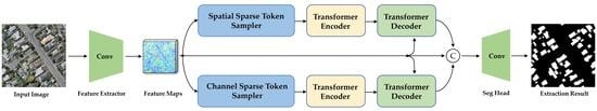
An overview of the proposed method. Our method consists of a CNN feature extractor, a spatial/channel sparse token sampler, a transformer-based encoder/decoder, and a prediction head. In the transformer part, when modeling the long-range dependency between different channels/spatial locations of the input image, instead of using all features vectors, we select the most important k s ( k s H W ) spatial tokens and k c ( k c C ) channel tokens. The sparse tokens greatly reduce the computational and memory consumption. Based on the semantic tokens generated by the encoder, a transformer decoder is employed to refine the original features. Finally, in our prediction head, we apply two upsampling layers to produce high-resolution building extraction results.
Remotesensing 13 04441 g002
Figure 3. 
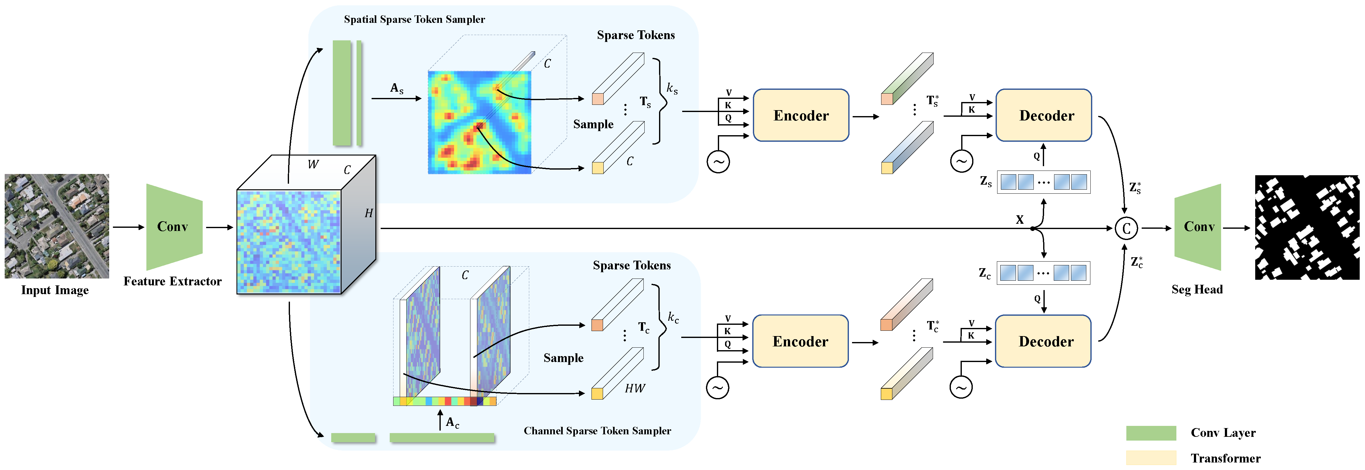
Samples from the Wuhan University Aerial Building Dataset (a) and the Inria Aerial Image Labeling Dataset (b). Buildings vary in size, shape and color, and may be occluded by trees.
Remotesensing 13 04441 g003
Figure 4. 
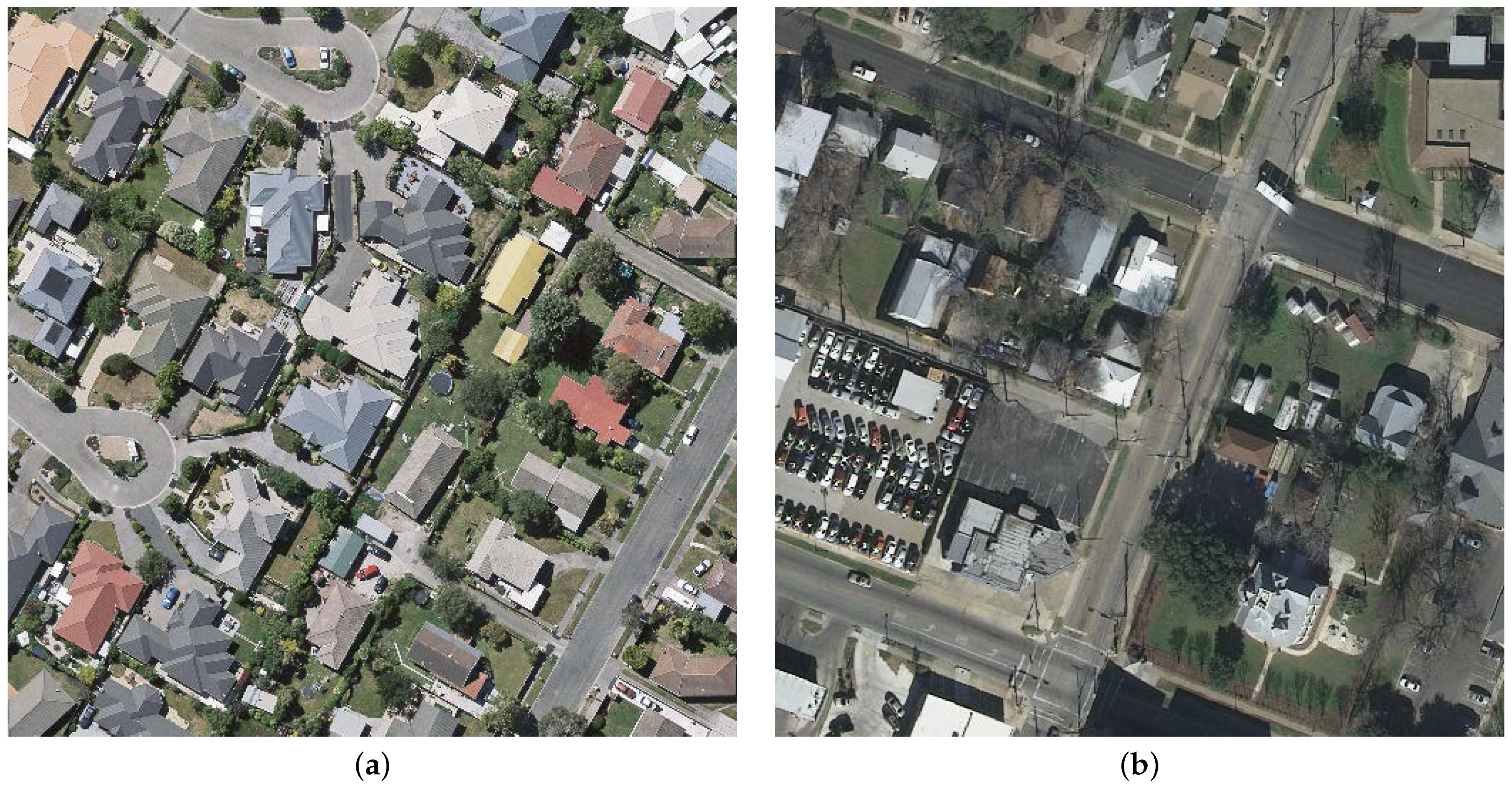
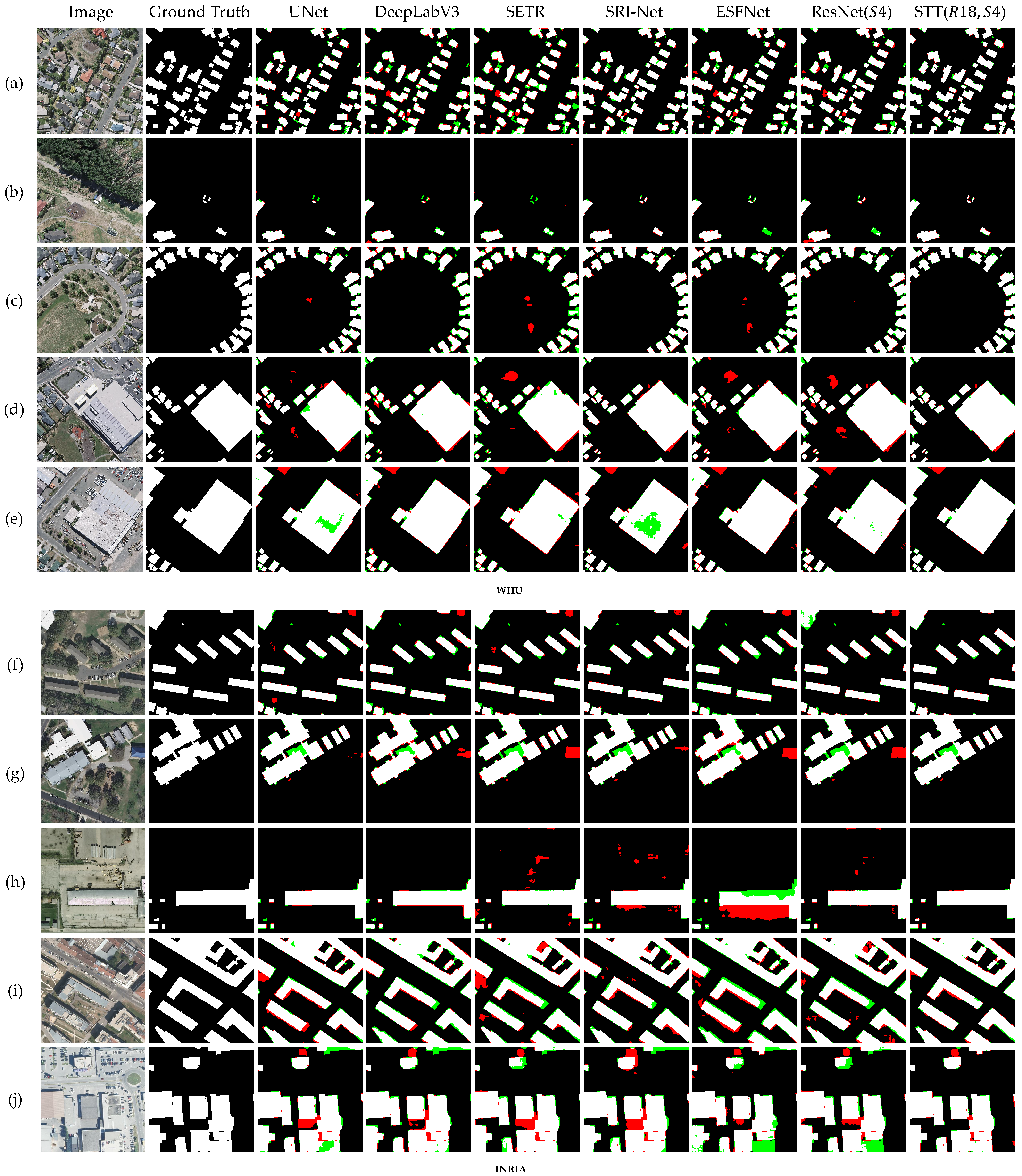
The results of different methods on samples from the WHU (ae) and INRIA (fj) building datasets are visualized. The figure is colored differently to facilitate viewing, with white representing true positive pixels, black representing true negative pixels, red representing false positive pixels, and green representing false negative pixels.
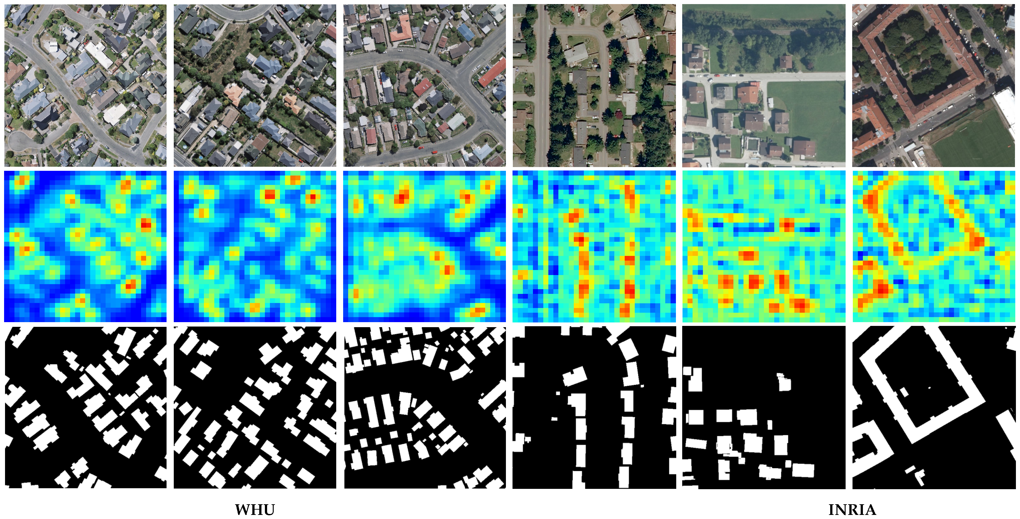
Remotesensing 13 04441 g004
Figure 5. Visualization of the spatial probabilistic maps. The rows from top to bottom are the input image, the spatial probabilistic map, and the ground truth label, respectively. High values are shown in red color and lower values are shown in blue. The heatmaps are taken from spatial map generator with pixel resolution of 32 × 32 .
Remotesensing 13 04441 g005
Figure 6. Visualization of channel probabilistic maps and their importance values. There are 4 samples from WHU and INRIA datasets. The left-most column shows input images. The right-most column shows the ground truth labels. The channel importance bars are plotted below for each images. The other 5 columns shows the heatmaps, which are taken from feature extractor with pixel resolution of 32 × 32 according to the channel probabilistic map. Here, we only pick the top-5 for visualization.
Remotesensing 13 04441 g006
Table 1. Details of network layers for generating the spatial and channel probabilistic maps.
ModuleInput SizeLayerOutput Size
Spatial map generator ( C , H , W ) Conv2d ( C , C / 4 , 3 ) ( C / 4 , H , W )
( C / 4 , H , W ) BN, LeakyReLU ( C / 4 , H , W )
( C / 4 , H , W ) Conv2d ( C / 4 , 1 , 3 ) ( 1 , H , W )
( 1 , H , W ) Sigmoid ( 1 , H , W )
Channel map generator ( C , H , W ) Conv2d ( C , C / 8 , H ) ( C / 8 , 1 , 1 )
( C / 8 , 1 , 1 ) BN, LeakyReLU ( C / 8 , 1 , 1 )
( C / 8 , 1 , 1 ) Conv2d ( C / 8 , C , 1 ) ( C , 1 , 1 )
( C , 1 , 1 ) Sigmoid ( C , 1 , 1 )
Table 2. Layers of the prediction head. We use the PixelShuffle layer [68] for upsampling. The up1 * layer is only applied when the last feature map size is 1 / 32 of the original resolution in ablation study. DoubleConv means two convolutional layers following by batch normalization and ReLU activation function.
ModuleInput SizeLayerOutput Size
up1 * ( C , H , W ) PixelShuffle ( 2 ) ( C / 4 , 2 H , 2 W )
( C / 4 , 2 H , 2 W ) DoubleConv ( C / 4 , C / 2 , C / 2 ) ( C / 2 , 2 H , 2 W )
up2 ( C / 2 , 2 H , 2 W ) PixelShuffle ( 4 ) ( C / 32 , 8 H , 8 W )
( C / 32 , 8 H , 8 W ) DoubleConv ( C / 32 , C / 8 , C / 8 ) ( C / 8 , 8 H , 8 W )
up3 ( C / 8 , 8 H , 8 W ) PixelShuffle ( 4 ) ( C / 128 , 32 H , 32 W )
( C / 128 , 32 H , 32 W ) DoubleConv ( C / 128 , C / 32 , C / 32 ) ( C / 32 , 32 H , 32 W )
predict ( C / 128 , 32 H , 32 W ) Conv2d ( C / 128 , C / 128 , 3 ) ( C / 128 , 32 H , 32 W )
( C / 128 , 32 H , 32 W ) BN, LeakyReLU ( C / 128 , 32 H , 32 W )
( C / 128 , 32 H , 32 W ) Conv2d ( C / 128 , 2 , 3 ) ( 2 , 32 H , 32 W )
Table 3. Computational complexity of different network architectures. PT: Plain Transformer layer. ST: Spatial Transformer in SST. CT: Channel Transformer in SST. Q , K , V are the query matrix, key matrix and value matrix in transformer layer respectively. Values of Q , K , V in the table are their dimensions. Complexity means the memory consumption. Let N q , N k , N v be the number of query, key, and value elements in the plain transformer, respectively. We have the following observations in general. N k = N v = N q for self-attention, and N k = N v N q for cross-attention.
ArchitectureQKVComplexity
PT (baseline) N q × d N k × d N v × d O ( N q N k d ) = O ( H 2 W 2 C )
ST Encoder (ours) k s × C k s × C k s × C O ( k s 2 C )
ST Decoder (ours) ( H W ) × C k s × C k s × C O ( H W k s C )
CT Encoder (ours) k c × ( H W ) k c × ( H W ) k c × ( H W ) O ( k c 2 H W )
CT Decoder (ours) C × ( H W ) k c × ( H W ) k c × ( H W ) O ( H W k c C )
Table 4. Ablation study of the context composing. We conduct experiments on different feature compositions before the final prediction head. ST: Spatial Transformer output, Z s * . CT: Channel Transformer output, Z c * . OM: Original feature Map before the transformer, X . †: Without auxiliary loss to generate probabilistic maps.
ModelSTCTOMWHUINRIA
IoUOAF 1 IoUOAF 1
ResNet18 ( S 4 ) ××84.5498.2991.4775.1495.8285.19
ResNet18 ( S 4 ) ××86.3698.6991.9376.0696.0085.78
SST ( R 18 ,   S 4 ) ××87.3998.6393.0276.3696.0386.00
SST ( R 18 ,   S 4 ) ×88.7598.7693.9976.5796.0986.11
SST ( R 18 ,   S 4 ) ××87.7398.6893.2576.4196.0386.04
SST ( R 18 ,   S 4 ) ×88.7798.7793.9976.8496.1286.32
SST ( R 18 ,   S 4 ) ×88.8298.7794.0476.9996.1486.43
SST ( R 18 ,   S 4 ) 89.0198.8094.1377.1296.1986.49
Table 5. Ablation study of our method SST ( R 18 ,   S 4 ) on the sparse token number (TN) in the spatial and channel transformers. “Throughput” means the number of images ( 512 × 512 pixels) processed per second at the inference phase.
TN in STTN in CTThroughputWHUINRIA
IoUOAF 1 IoUOAF 1
416319487.7398.6893.2576.7296.1086.24
1616315888.4898.7693.7776.8596.1386.32
6416313489.0198.8094.1377.1296.1986.49
25616231589.0798.8194.1777.1896.2086.52
10241668888.9698.7994.1177.0296.1786.45
644318987.8098.6993.3076.7396.1286.25
648315788.5998.7493.9176.9796.1286.43
6432310489.0598.8194.1577.2896.2186.60
6464307789.0498.8194.1677.0996.1786.50
44323286.8398.7392.3476.6996.1086.23
168314488.1898.7393.5576.7896.1286.26
25632220989.1198.8094.2077.2196.1886.56
10246466588.9598.7994.1176.9796.1486.41
Table 6. Ablation study of the position embeddings (PE) in the spatial and channel transformer on the two datasets. The evaluation is conducted on both the transformer encoder and the transformer decoder.
Spatial TransformerChannel TransformerWHUINRIA
PE in EncoderPE in DecoderPE in EncoderPE in DecoderIoUOAF 1 IoUOAF 1
××××88.4198.7593.7676.7996.1186.28
××88.8398.7994.0276.9496.1286.38
××88.8098.7794.0177.0696.1786.46
89.0198.8094.1377.1296.1986.49
Table 7. Evaluations on different ways of generating token probabilistic maps in our method. †: Without auxiliary loss to generate probabilistic maps.
MethodWHUINRIA
IoUOAF 1 IoUOAF 1
ResNet18 ( S 4 ) 84.5498.2991.4775.1495.8285.19
M a x 86.3598.4692.6476.6696.0786.21
M e a n 85.6598.4292.1475.7195.9685.69
P r e d i c t * 85.7298.4292.1776.0696.0085.78
P r e d i c t 89.0198.8094.1377.1296.1986.49
Table 8. Accuracy of our method SST ( R 18 ,   S 4 ) with different loss balancing factors α , and w/ or w/o using pretraining.
α PretrainWHUINRIA
IoUOAF 1 IoUOAF 1
1×88.0998.7193.5876.4496.0786.05
0.1×88.5798.7493.9076.5096.0886.07
0.01×88.7198.7793.9676.7896.1386.28
0.001×88.6698.7593.9576.9596.1486.39
0.0001×88.2498.7193.6876.6496.0986.19
188.3598.7393.7676.5896.0786.14
0.188.7798.7893.9976.7696.1186.26
0.0188.9098.7894.0776.9996.1486.43
0.00189.0198.8094.1377.1296.1986.49
0.000188.8498.7994.0376.6996.1086.21
Table 9. Comparison with some well-known image labeling methods and state-of-the-art building extraction methods on the WHU and INRIA building datasets. UNet, SegNet, DANet, and DeepLabV3 are commonly used methods for segmentation tasks in CNN framework. SETR is a transformer-based method for segmentation. The methods mentioned in the second row are all based on the CNN framework for specific building extraction tasks. To validate the efficiency, we report number of parameters (Params.), multiply-accumulate operations (MACs) and images with 512 × 512 pixels per second on a 2080Ti GPU (Throughput).
ModelParams.(M)MACs(G)ThroughputWHUINRIA
IoUOAF 1 IoUOAF 1
UNet [41]17.27160.4882387.5298.6593.1177.2996.2586.56
SegNet [42]29.44160.5674885.1398.3691.7476.3296.1085.83
DANet [63]17.3922.33578781.2297.8289.5776.0295.9485.80
DeepLabV3 [44]15.3120.06716280.6997.7689.2473.9095.5484.39
SETR [27]64.5634.46110575.9297.1387.7570.3494.8782.06
DAN-Net [62]1.9875.2918387.6998.8092.8176.6396.0886.17
MAP-Net [46]24.0294.3823188.9998.8294.1276.9196.1386.34
SRI-Net [38]13.86176.6425788.8498.7393.9876.8496.1286.32
BRRNet [12]17.341255.1249189.0398.8194.1477.0596.4786.61
ESFNet [56]0.5589.26971683.8198.1691.1371.2895.0882.47
VGG16 ( S 5 , B N ) 17.8892.24195285.2098.3591.7777.9096.3187.02
VGG16 ( S 4 , B N ) 7.8581.96207886.2898.4992.4777.9996.3687.08
SST ( V 16 ,   S 4 ,   B N ) (Ours)17.0982.43163289.3798.8494.1179.1596.5687.81
ResNet18 ( S 5 ) 12.1213.37392484.1498.1891.3374.8095.7485.00
ResNet18 ( S 4 ) 2.8410.31438584.5498.2991.4775.1495.8285.19
SST ( R 18 ,   S 4 ) (Ours)12.0110.71313489.0198.8094.1377.1296.1986.49
ResNet50 ( S 5 ) 38.4970.39131186.4798.5092.5078.0496.3487.08
ResNet50 ( S 4 ) 9.3751.65146286.8898.5092.9578.1296.4087.13
SST ( R 50 ,   S 4 ) (Ours)18.7452.25116690.4898.9794.9779.4296.5987.99
Publisher’s Note: MDPI stays neutral with regard to jurisdictional claims in published maps and institutional affiliations.

