Article

Monitoring Metropolitan Growth Dynamics for Achieving Sustainable Urbanization (SDG 11.3) in Kolkata Metropolitan Area, India

1
Department of Geography, Haldia Government College, Vidyasagar University, Haldia 721657, India
2
School of Environment, Education & Development, University of Manchester, Manchester M13 9PL, UK
3
Department of Architecture and Regional Planning, Indian Institute of Technology, Kharagpur 721302, India
4
Natural Resources and Ecosystem Services Area, Institute for Global Environmental Strategies, Hayama 240-0115, Kanagawa, Japan
5
Department of Civil Engineering, College of Engineering, King Khalid University, Abha 61421, Saudi Arabia
6
Department of Civil Engineering, High Institute of Technological Studies, Mrezgua University Campus, Nabeul 8000, Tunisia
7
Faculty of Environmental Earth Science, Hokkaido University, Sapporo 060-0810, Japan
*
Author to whom correspondence should be addressed.
Remote Sens. 2021, 13(21), 4423; https://doi.org/10.3390/rs13214423
Submission received: 20 September 2021 / Revised: 15 October 2021 / Accepted: 29 October 2021 / Published: 3 November 2021

Abstract

:
The mass accumulation of population in the larger cities of India has led to accelerated and unprecedented peripheral urban expansion over the last few decades. This rapid peripheral growth is characterized by an uncontrolled, low density, fragmented and haphazard patchwork of development popularly known as urban sprawl. The Kolkata Metropolitan Area (KMA) has been one of the fastest-growing metropolitan areas in India and is experiencing rampant suburbanization and peripheral expansion. Hence, understanding urban growth and its dynamics in these rapidly changing environments is critical for city planners and resource managers. Furthermore, understanding urban expansion and urban growth patterns are essential for achieving inclusive and sustainable urbanization as defined by the United Nations in the Sustainable Development Goals (e.g., SDGs, 11.3). The present research attempts to quantify and model the urban growth dynamics of large and diverse metropolitan areas with a distinct methodology considering the case of KMA. In the study, land use and land cover (LULC) maps of KMA were prepared for three different years (i.e., for 1996, 2006, and 2016) through the classification of Landsat imagery using a support vector machine (SVM) classification approach. Then, change detection analysis, landscape metrics, a concentric zone approach, and Shannon’s entropy approach were applied for spatiotemporal assessment and quantification of urban growth in KMA. The achieved classification accuracies were found to be 89.75%, 92.00%, and 92.75%, with corresponding Kappa values of 0.879, 0.904, and 0.912 for 1996, 2006, and 2016, respectively. It is concluded that KMA has been experiencing typical urban sprawl. The peri-urban areas (i.e., KMA-rural) are growing rapidly, and are characterized by leapfrogging and fragmented built-up area development, compared to the central KMA (i.e., KMA-urban), which has become more compact in recent years.

Graphical Abstract

1. Introduction

Detecting and quantifying urban expansion patterns and processes are standard practices in urban sprawl studies [1,2,3,4]. According to Wilson and Chakraborty [5], studying the physical characteristics of urban growth as a pattern of urban development is one of the most common approaches in defining urban sprawl. Change in the urban built-up area, i.e., all human-made structures and impervious surfaces, is typically employed as an efficient and straightforward parameter for quantifying urban expansion and urban sprawl [6,7,8].
Urban expansion can be efficiently monitored and modeled using remote sensing (RS) and geographic information systems (GIS) tools, which are cost-effective and technologically robust [4,9,10]. Researchers have developed various indices and models coupled with RS-GIS to quantify patterns and processes of urban growth in cities. Change detection using multispectral and temporal RS images is a popular method for mapping the spatiotemporal dynamics of land cover in an area. Based on these land-cover-change maps, Shannon’s entropy ( H n ) has proven its usefulness and reliability in quantifying the degree of compactness and dispersion of urban growth in absolute scale [4,9,11,12,13]. On the other hand, landscape metrics or spatial metrics [14], though initially emerging in the field of ‘landscape ecology’, are also increasingly being applied to quantify and monitor patterns of physical urban growth on a relative scale [15,16]. However, the use of a single metric may not reflect the actual reality, as each metric tends to have certain limitations. Researchers often use H n in combination with other landscape metrics to establish and explain the results with greater certainty [4].
The H n and other different landscape metrics have been applied at various spatial and administrative levels within city systems to analyze urban growth. Some studies consider a total city-system as the unit of analysis [4,17]. Others have considered smaller parts of the whole city as units of analysis, such as ward level in a city [4,18,19], arbitrarily created sub-zones within a city system [4,12,20], or concentric circles of specific width(s) encircling a city center [3]. Moreover, zonal and city-level units are often considered at the same time to investigate urban growth effectively [4,21]. The Kolkata Metropolitan Area (hereafter KMA) depicts a very diverse structure. Metropolises in India consist of statutory urban areas in the central part and rural or peri-urban areas outside of the statutory urban areas. Such central and peripheral regions within the same metropolitan system have different administrative bodies, economic structures, population composition, etc. Notably, the increase in size and population growth varies substantially from the urban core to the rural periphery [4]. Therefore, it is necessary to analyze, quantify and monitor such built-up growth dynamics at rural and urban levels within the same metropolitan system to achieve the inclusive and sustainable urbanization target as defined by the United Nations in Sustainable Development Goal (SDG) 11.3 and to make urban planning more realistic [22,23].
The present study attempts to quantify the urban growth dynamics of the KMA, India, using an integrated RS-GIS application, and to prepare recommendations for inclusive and sustainable urbanization (SDG 11.3). For this purpose, a zoning approach has been used to examine the urban growth dynamics of KMA at three different spatial levels, namely KMA, KMA-urban, and KMA-rural [4,24]. Multispectral and temporal Landsat Thematic Mapper (TM) and Operational Land Imager (OLI) imageries were considered over 20 years, i.e., between 1996 and 2016. Post-classification comparison was applied as a change detection technique for analyzing spatiotemporal dynamics of land cover in the metropolitan area driven by rapid built-up growth [25,26]. The H n was employed to quantify the degree of compactness and dispersion of the physical growth of KMA on an absolute scale. Moreover, a set of other landscape metrics were applied to analyze the pattern, fragmentation, and heterogeneity of the physical growth in KMA and their dynamics over time on a relative scale. Finally, a set of policy recommendations and measures has been proposed for achieving SDG 11.3. The current study represents a unique contribution to urban landscape heterogeneity analysis and urban growth dynamics concerning the proposed zoning approach, areal coverage under the study, and the use of landscape metrics. The following objectives were framed to address the research questions considered:
  • Classifying land use and land cover (LULC) maps of KMA by applying machine learning using a support vector machine (SVM) approach.
  • Implementing post-classification comparison-led change detection analysis concerning spatiotemporal dynamics in class area, percentage, and growth of LULC in KMA.
  • Quantifying the spatiotemporal pattern of urban growth in KMA employing the selected landscape metrics.
  • Measuring the degree of compactness and dispersion in urban growth and determining the presence and degree of urban sprawl in KMA with a black-and-white scale applying the H n approach.
  • Preparing a set of policy recommendations and measures from the finding of the study for achieving sustainable urbanization (SDGs 11.3) and capacity for participatory, integrated, and sustainable planning and management for KMA.

2. Materials and Methods
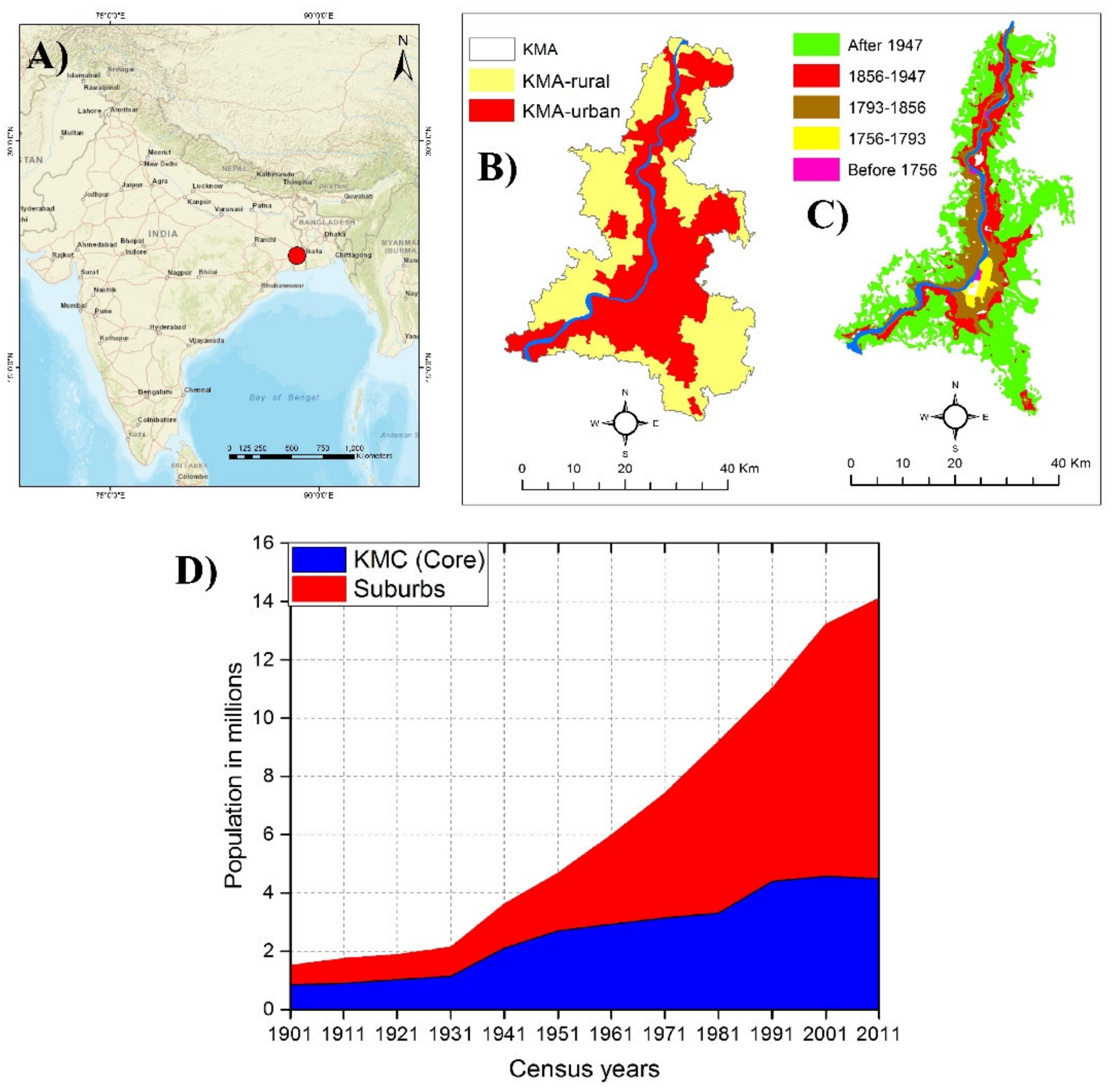
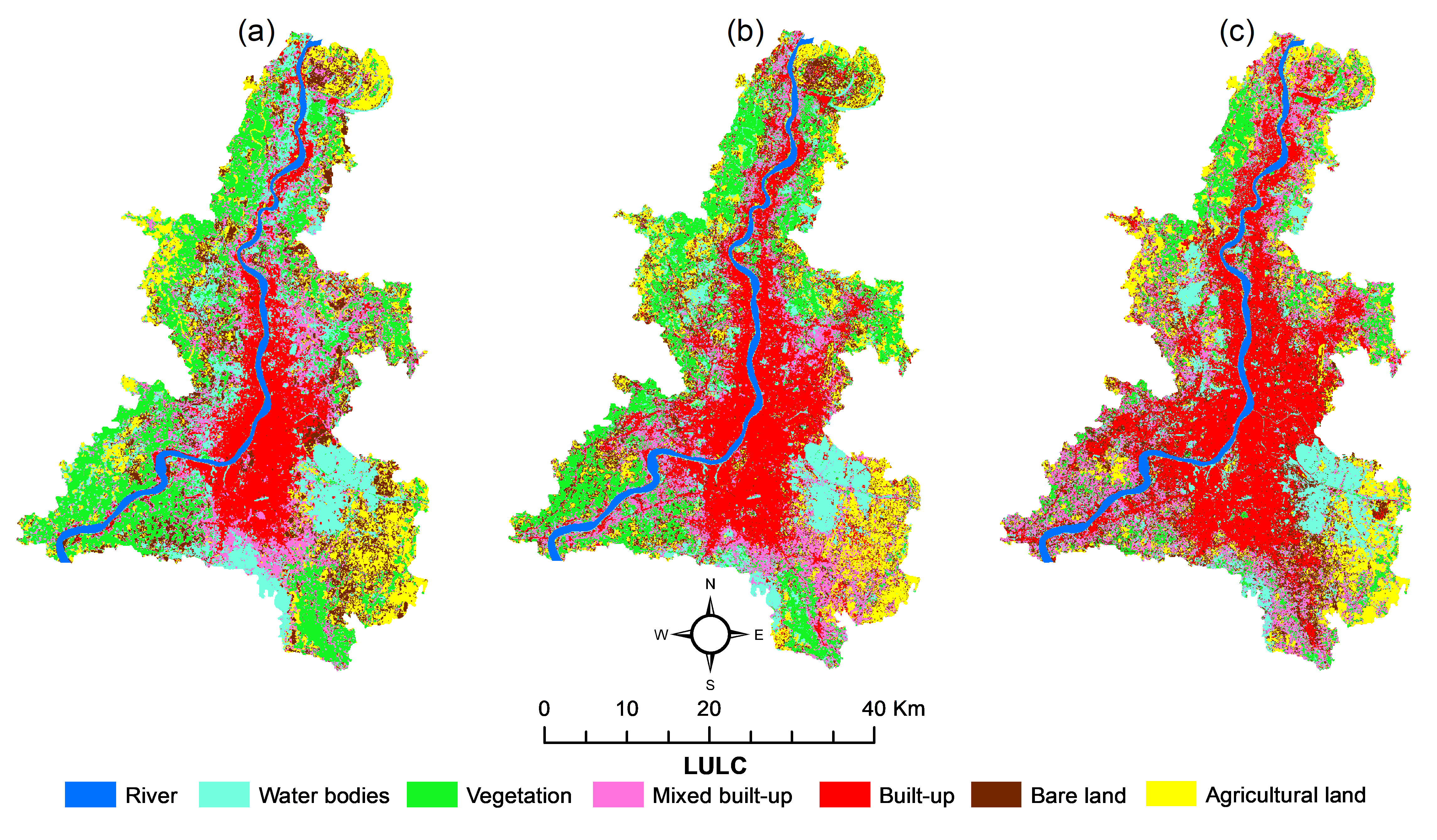
2.1. Research Area

This study focused on the KMA as a case study for spatiotemporal assessment and quantification of urban growth dynamics for the achievement of sustainable urbanization (SDG 11.3) in developing countries. Kolkata is one of the important fast-growing million-population-level cities in eastern India with major consequences of rapid urban growth within the periphery area and sprawl development [27]. Over the last two decades, the KMA has been growing at an annual rate of about 2% with increase of the population from 9.19 million in 1981 to 13.21 million in 2001 [28], and to 14.11 million in 2011. This accumulation of population in the suburbs has accelerated peripheral urban growth in KMA, particularly during the last few decades, as shown in Figure 1. The KMA occupied approximately 361 sq. km during independence. However, it expanded in area to 1350 sq. km and 1851.41 sq. km by 1991 and 2001, respectively. Presently, KMA extends over an area of 1886.67 km2 [4,29,30]. The metropolitan area’s growth has been unchecked as suburbanization has rapidly engulfed agricultural land, vegetation cover, and water bodies along the periphery.
The present study used a zoning approach to assess the urban growth dynamics in KMA. The zoning approach examined the growth dynamics in KMA at three different spatial levels, namely KMA (the whole metropolitan area), KMA-urban (all statutory urban areas within KMA), and KMA-rural (rural areas and census towns) [4,24], as shown in Figure 1.

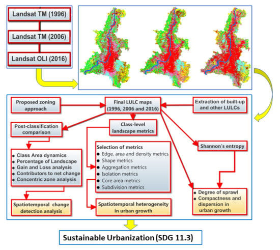
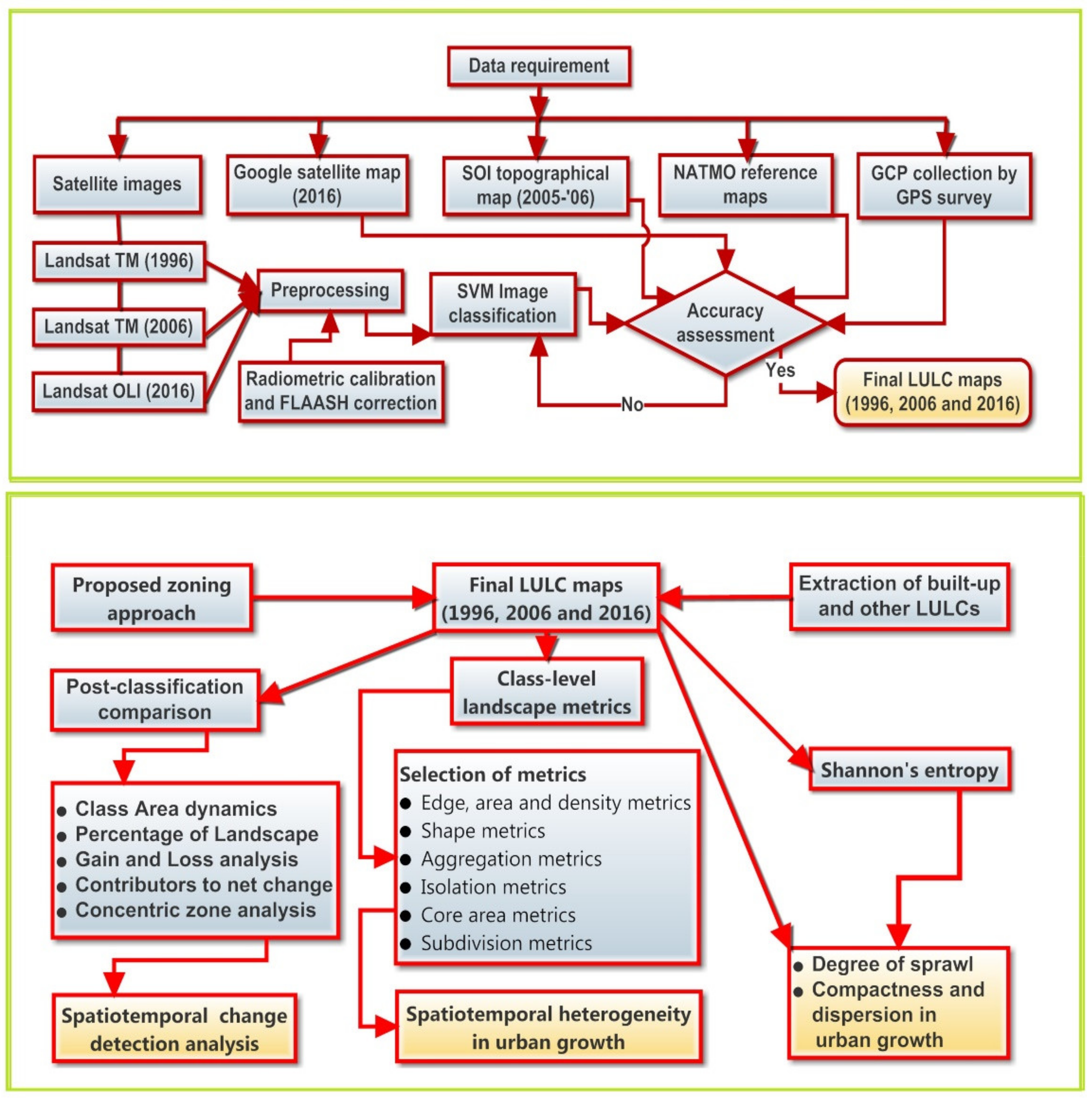
2.2. Data Source and Methodology

The present study used remotely sensed Landsat satellite images as the prime database for three specific points of time, i.e., 1996, 2006, and 2016 (the details of acquired satellite images are provided in Appendix A). All three images were classified into six classes, namely built-up, mixed built-up, water bodies, vegetation, agricultural land, and bare or barren land, applying the SVM classification approach, to reflect the major land-use types of KMA (LULC class definitions are given in Appendix B). The SVM-generated final LULCs for 1996, 2006, and 2016 (Appendix C) were taken as the input databases for further analysis. The vector map of KMA depicting the zoning approach was also taken as an input in this study. The methodology adopted in the present study is represented by a flowchart (Figure 2).
In the present study, a total of 400 random points was generated for each of the classified maps separately, applying a stratified random sampling technique with a minimum threshold of 50 points for each category for assessing accuracies of the classified images for 1996, 2006, and 2016. The achieved overall accuracies for the classified imageries were found to be 89.75% for 1996, 92.00% for 2006, and 92.75% for 2016. The Kappa index of statistical agreement for all the three classified maps, i.e., 1996, 2006 and 2016, were observed at 0.879, 0.904, and 0.912, respectively. Hence, all the observed Kappa agreements in the present study can be described as close to ideal [31]. Therefore, all the achieved accuracies found in the present study were satisfactory and acceptable. Table 1 presents a summary of the accuracy assessment; Appendix D shows the detailed error relating to the accuracy assessment of the classified LULC maps for 1996, 2006, and 2016.
Change detection refers to the process of determining an aerial change in land cover based on co-registered multi-temporal RS data. The present study applied the post-classification comparison-led change detection technique [25,26] for analyzing land cover dynamics in the metropolitan area of KMA with the adopted zoning methodology, i.e., KMA, KMA-urban, and KMA-rural during 1996–2006, 2006–2016, and 1996–2016. The applied change detection technique provides ‘from-to’ change information and the kind of land cover transformations that have occurred over a particular period and can be readily derived and mapped [32]. The change detection analysis undertaken considered the spatiotemporal dynamics in the class area (CA), the percentage of landscape (PLAND), decadal growth, gain and loss, net change, and contributors to the net change in the LULC of KMA.

2.3. Landscape Metrics

Landscape metrics are quantitative indices used to quantify the structure, pattern, and spatial heterogeneity of patches and landscapes within a designated landscape boundary [14,33]. Landscape metrics can be spatially explicit patch-based and pixel-based indices as well as spatially non-explicit aggregate measures [15,34,35]. There are a large number of metrics that different scholars have used. The metrics mentioned above can be applied at the patch level, class level, and landscape-level, or all three levels, to measure heterogeneity in the pattern of the landscape.
The application of spatial metrics and RS and GIS in urban studies, especially in the quantification, mapping, and modeling of urban growth and sprawl, is a recent practice and is still at an exploratory stage. However, many studies have applied the metrics in the field of urban studies. Several of these studies, such as Geoghegan et al. [36], Alberti and Waddell [37], Parker et al. [38], Herold et al. [15], Cabral et al. [16], Taubenböck et al. [38], Zhang [39], Pham et al. [40], Tian et al. [41], Kong et al. [42], Lü et al. [43], and Wu et al. [44] have applied and suggested specific metrics to use in urban morphology and to quantify structures and patterns of urban growth and urban sprawl considering effectiveness and scaling effects.
Even though spatial metrics have essential applications in quantifying urban growth and urban sprawl [45], there are some challenges related to the application of spatial metrics. Some of the metrics are correlated and, therefore, may contain redundant information [46,47]. According to Parker et al. [37], there is no standard set of metrics best suited for urban studies, and the relevance of the metrics varies with the objectives under study.
Though the selection of metrics has been difficult and there is a lack of metrics best suited for quantifying urban growth, some studies, such as Alberti and Waddell [36], Parker et al. [37], and Araya and Cabral [48], have compared a wide variety of different metrics and suggested those metrics suitable for analyzing urban land cover changes.
In the present study, a set of class-level landscape metrics have been selected based on the principles that they are: (1) important both in theory and practice, (2) interpretable, (3) minimally redundant, and (4) easily computed. The selected class-level metrics were CA, PLAND, number of patch (NP), patch density (PD), largest patch index (LPI), mean patch size (AREA_MN), mean shape index (Shape_MN), perimeter area fractal dimension (PAFRAC), total core area (TCA), core area percentage of landscape (CPLAND), mean Euclidean nearest neighbor (ENN_NN), mesh size (MESH), aggregation index (AI), normalized landscape shape index (nLSI), percentage of like adjacency (PLADJ), and clumpiness index (CLUPMY).
In the present research, the selected class-level metrics were applied to quantify the heterogeneity in spatial patterns and temporal dynamics of the urban expansion in KMA using the adopted zoning approach on a relative scale. The open-source FRAGSTATS package [49] with an 8-cell neighborhood rule was employed to compute the metrics. The thematic LULC maps of KMA of 1996, 2006, and 2016 were used as input databases to compute the metrics.

2.4. Shannon’s Entropy ( H n )

The measure of H n is based on entropy theory, which was initially developed for the measurement of information [50]. Entropy can be applied in measuring the concentration and dispersion of a phenomenon. As a result, the H n index has been widely used in various fields, including urban studies. It is an important and reliable measure for deriving the degree of compactness and dispersion of urban growth [11,19,51,52] and quantifying urban sprawl on an absolute scale. The H n is calculated by Equation (1),
H n = i = 1 n p i log ( 1 p i )
where, pi is the proportion of a geophysical variable in the ith zone, and n refers to the total number of zones. The entropy value ranges from 0 to log(n). A value closer to zero indicates a very compact distribution, whereas a value closer to log(n) indicates the distribution is dispersed. The halfway value of log(n) is considered as the threshold value; hence, a city with an entropy value exceeding the threshold value can be described as a sprawling city [4,13].
The magnitude of the index signifies the level of sprawl. The measure of entropy is superior to other measures of spatial statistics, such as Gini’s and Moran’s coefficients, as these are affected by the size and shape, and the number of sub-units [51,52,53,54]. According to Bhatta [47], the entropy value is a robust measure since it can identify urban sprawl in black-and-white terms. In this study, using built-up density (ha/sq km) as the geophysical variable, the H n index was separately derived for KMA, KMA-urban, and KMA-rural [4,22].
Yeh and Li [52] argued that entropy values for different years could be used to show the difference in entropy between t-1 and t-2 to indicate the magnitude of change in entropy as a result of change in a spatial phenomenon for the specific period, as in Equation (2),
Δ H n = H n t 2 H n t 1
where, Δ H n is the magnitude of change in entropy between the period t-1 and t-2. Using this approach, urban growth and urban sprawl can be analyzed as a temporal process. The magnitude of change in entropy signifies whether a city is becoming more dispersed or compact over time.

3. Results

3.1. CA and PLAND Analysis

KMA has undergone a substantial LULC transformation as a result of continuous and rapid built-up expansion over the last few decades. The spatial overview of built-up expansion (both built-up and mixed built-up), with its temporal dynamics during 1996–2016, is presented in Figure 3.
The magnitudes of different LULCs, i.e., CA over KMA, KMA-urban, and KMA-rural in 1996, 2006, and 2016 are presented in Appendix E, and their corresponding temporal growth during 1996–2006, 2006–2016, and 1996–2016 is presented in Table 2. Figure 3 shows the corresponding proportions (%) of the LULCs, i.e., PLAND, in the respective years for the three proposed zones in KMA. In 1996, of the KMA area a total of 31.65% comprised built-up cover, with 16.05% urban built-up cover and 15.6% peripheral mixed built-up cover, followed by vegetation, water bodies, agricultural land, and bare land, with area cover of 23.17%, 16.4%, 15.85%, and 12.94%, respectively, as shown in Figure 3. However, the scenario differed significantly when we considered KMA-urban and KMA-rural separately along with the whole KMA. In 1996, KMA-urban and KMA-rural comprised approximately 49.43% and 15.07% of the PLAND, respectively, of built-up and mixed built-up land cover. KMA-rural possessed an insignificant PLAND of mixed built-up cover, i.e., 2.13% in 1996, illustrating a lower rate of peripheral urban expansion at that time. In 2006, the PLAND of total built-up (built-up and mixed built-up) was 39.74%, 60.25%, and 21.22% in KMA, KMA-urban, and KMA-rural, respectively. In 2016, the PLAND of built-up and mixed built-up together was 49.43%, 66.77%, and 33.04% in KMA, KMA-urban, and KMA-rural, respectively. Hence, KMA-rural has exhibited a steady and sharp gain in the PLAND of total built-up recently, increasing from only 15.07% in 1996 to 33.04% in 2016. This rate of increase has been more than double that of KMA-urban, where the total built-up cover changed from 49.43% to 66.77% during the same period, explaining the phenomenon of large-scale new built-up development along the periphery. In the case of KMA-urban, the PLAND of built-up increased from 30.74% in 1996 to 53.73% in 2016, while the PLAND of mixed built-up decreased from 18.69% to 13.04% in the period signifying the in situ process of conversion of mixed built-up into built-up as a result of built-up densification and infill processes. However, the scenario of KMA-rural differs substantially from that of KMA-urban. KMA-rural depicts a significant increase in the PLAND of both built-up and mixed built-up from 1996 to 2016, when the PLAND of built-up and mixed built-up changed from 2.13% to 11.02% and from 12.94% to 22.03%, respectively. The higher PLAND of mixed built-up, with its higher temporal gain in KMA-rural, indicates the phenomenon of low density, dispersed, and rapid new built-up development there known as urban sprawl.
The analysis of the temporal pattern of built-up growth over KMA, showed that during 1996–2006, the built-up area grew rapidly by 49.16% at a rate of approximately 5% per year; however, the rate of growth slowed to 31.32% during the next decade, i.e., 2006–2016 (Table 2). In the case of mixed built-up over KMA the decadal growth rate increased from 1.24% to 10.48% between 1996–2006 and 2006–2016, respectively. The phenomena of annual and decadal growth rate over KMA-urban and KMA-rural reflects substantial dynamics as compared to the whole KMA. In KMA-rural, the decadal built-up growth was 196.82% during 1996–2006, increasing at a rate of approximately 20% per year. This was much higher than its counterpart KMA-urban, where the growth rate was only 38.35% for the same period. During 2006–2016, though the rate of built-up growth in KMA-rural declined, it was higher than that of KMA-urban. The CA of mixed built-up grew negatively in KMA-urban during the study period by −5.17% during 1996–2006 and −26.44% during 2006–2016, whereas in KMA-rural, it increased by 10.19% and 54.89%, respectively. Hence, KMA-rural demonstrates a rapid CA growth of built-up and mixed built-up, signifying the occurrence of urban sprawl along the outskirts (Table 2).
There have been noteworthy dynamics in agricultural land over KMA as a result of incessant built-up spread. KMA comprised about 15.85% of the PLAND of agricultural land in 1996, which fell a little to 14.55% in 2016. Even though KMA-rural has had a much higher PLAND of agricultural land than KMA-urban over time, both of them demonstrated small losses in the PLAND during the study period. The PLAND of agricultural land changed from 7.84% in 1996 to 6.16% in 2016 in KMA-urban, while in KMA-rural, the same altered from 22.26% in 1996 to 21.64% in 2016 (Figure 4). The scenario of the decadal growth of the PLAND reveals a more substantial variation at different spatial and temporal scales. During the study period, i.e., 1996-2016, the CA of agricultural land grew negatively, which dipped even more during 2006–2016, i.e., by −9.58% at a negative rate of approximately −1% per year. The growth of the CA was also found to be negative over KMA-urban and KMA-rural. During 1996–2016, the CA in KMA-urban changed negatively by −21.46%, while the change was approximately −4.25% in KMA-rural, much less in comparison to KMA-urban (Table 2). Therefore, during the study period, the CA of agricultural land shrank much more rapidly over the urban areas of KMA than its periphery or peri-urban areas.
The spatial and temporal dynamics were also evident in the PLAND and CA of vegetation cover over the KMA. Figure 4 shows that over the KMA, the vegetation cover has been decreasing steadily and rapidly. The PLAND of vegetation cover dropped to 10.0% in 2016 from 23.17% in 1996; the loss in the PLAND was even more prominent during 2006–2016 in comparison to the period 1996–2006. The magnitude of shrinkage in the PLAND was also higher over both KMA-urban and KMA-rural. Between 1996 and 2016, the vegetation cover PLAND dropped to 4.51% from 16.89% in KMA-urban, and from 29.55% to 14.94% in KMA-rural. However, in the last decade, the drop in the PLAND in KMA-rural was higher than for KMA-urban, signifying the recent built-up sprawl over the KMA-rural at the cost of vegetation cover. The decadal growth trend of the CA of vegetation cover reflects that during 1996–2006, the KMA-urban lost its vegetation cover by −33.65%, while there was a reduction of −11.72% for KMA-rural. During 2006–2016, KMA-urban experienced negative growth of −59.79% in vegetation cover, while it was −40.98% in the case of KMA-rural. Overall, KMA vegetation cover was reduced by −56.91% during the study period as a consequence of uncontrolled built-up expansion in the metropolitan area.
The PLAND of water bodies showed a fluctuating pattern in the metropolitan area. During 1996–2016, the PLAND of water bodies dropped to 13.85% from 16.40%. During the same period, in KMA-urban and KMA-rural, the PLAND of water bodies reduced from 15.81% to 11.13% and from 17.03% to 16.21%, respectively. However, a minor variability in the PLAND of water bodies was observed during 2006–2016, which might have been due to different dates of the deployed satellite imageries and residual errors in image classification. Figure 4 shows that since 2006 onwards, the conversion of water bodies into urban impervious land cover has reduced. The decadal growth analysis (Table 2) reveals that there has been a 15.72% shrinkage in water bodies over the study period of 20 years (i.e., 1996–2016) in the metropolitan area, while it reduced by −29.63% and −3.43% for KMA-urban and KMA-rural, respectively, over the same period.
Unlike other LULCs, minor spatiotemporal dynamics were evident in the case of the PLAND and CA of bare land in the metropolitan area. There was a seemingly stable trend in the PLAND of barren land in KMA, approximately level at 12% during the study period. A closely similar pattern in the PLAND was observed for KMA-urban. However, in KMA-rural, there was a loss of approximately 2% in the PLAND of bare land during the study period. Table 2 shows that during the study period, i.e., 1996–2016, the metropolitan area experienced negative growth in the land cover of −2.86%, while a reduction of −13.01% was observed in KMA-rural. This signifies that the impact of built-up expansion over KMA-rural, i.e., peripheral KMA, has been higher than for KMA-urban.

3.2. Gain and Loss Analysis

The gain and loss analysis reveals losses for all types of land cover, excluding built-up and mixed built-up, during the study period, i.e., 1996–2016. During the period, the land cover of vegetation gained about 4953 ha as new areas. However, during the same period, approximately 33,370 ha were lost from the existing areas as a result of conversion to other types of land cover, as shown in Figure 5. The process of land cover transformation resulted in a net loss in vegetation cover of around 28,416 ha of its area, amounting to negative growth of −62.08% during 1996–2016. Net losses for bare land, water bodies, and agricultural land were also reported at 7764 ha, 6984 ha, and 5930 ha leading to a reduction in the area of the land covered by 26.02%, 23.35%, and 18.86%, over the same period (Figure 5 and Figure 6). In contrast, the continuous urbanization at the cost of non-built-up land cover led to rapid growth in urban built-up areas. During the period, built-up and mixed built-up cover increased by around 30557 ha and 18538 ha, amounting to 128.24% and 158.50% growth, respectively (Figure 5 and Figure 6). However, there was a loss of 9550 ha in mixed built-up areas, which was evidently due to the conversion of mixed built-up into built-up areas. The spatial view of gains, losses, and persistence of different land covers is presented in Figure 5.

3.3. Contributors to the Net Change in the LULCs

The contributors with their roles in the net areal loss of land covers are shown in Figure 7. The net areal loss in water bodies, agricultural land, vegetation, and bare land were found to be primarily caused by the growth in mixed built-up cover followed by the built-up cover during the study period. The most significant contributor in the net change of water bodies appears to be mixed built-up cover, at approximately −34.45%, followed by built-up cover (−26.88%). However, vegetation and agricultural land use had a small positive contribution to the net change of water bodies (Figure 7). The negative contributions of mixed built-up and built-up land cover were −128.85% and −27.67% to the areal loss of vegetation cover, −30.70% and −12.63% to the areal loss of agricultural land, and −43.16% and −22.45% to the areal loss of bare land, respectively. Therefore, the growth and expansion of built-up and mixed built-up areas have been the most significant drivers behind land cover dynamics in the metropolitan area. Moreover, the land cover by mixed built-up appears to be the biggest threat to land covers such as agricultural land, water bodies, vegetation, and bare land as they are each largely being converted into urban mixed built-up areas. This has apparently been due to the fast and haphazard urban expansion along the periphery induced by large-scale urban sprawl and its encroachment on other land covers.
The land cover of mixed built-up contributed to a positive net change of built-up areas by 78.64%, followed by water bodies (21.42%), bare land (17.93%), vegetation (14.41%), and agricultural land (9.59%). The net change in mixed built-up was positively contributed by all types of land cover other than built-up. The contribution of built-up in the net change of mixed built-up was −38.60%. This explains the incidence of the rapid and massive conversion of mixed built-up into built-up cover with time. The land cover of vegetation was the most significant contributor to the net positive change of mixed built-up amounting to 32.92%, followed by water bodies, bare land, vegetation, and agricultural land, as shown in Figure 8.

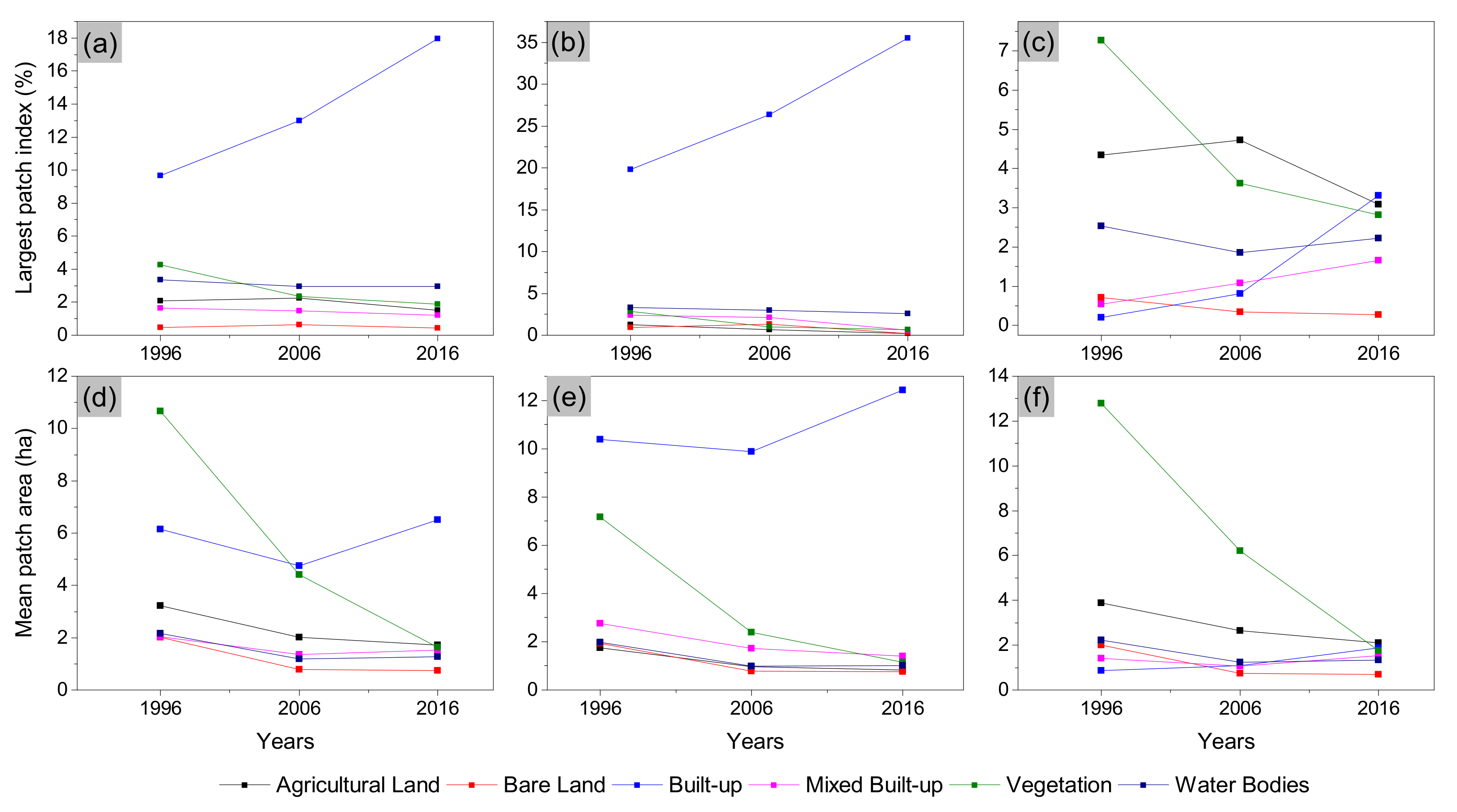
3.4. Landscape Metrics Analysis

Landscape metrics were computed for the classified images of KMA for 1996, 2006, and 2016. The adopted zoning and concentric zone approaches were used in the analysis of the results of the landscape metrics. Figure 9 presents the results of NP and PD with their spatiotemporal trend. In KMA, the NP of built-up increased from 4525 in 1996 to 8744 in 2006; however, it declined a little to 8366 in 2016. The same trend was observed in the case of mixed built-up cover. This explains why the degree of fragmentation in urban growth measured by NP of built-up decreased at the metropolitan level, particularly after 2006. A significant degree of spatiotemporal dynamics in NP was observed both in KMA-urban and KMA-rural. KMA-urban, which comprises all statutory urban areas within KMA, showed an almost stationary trend in built-up NP after 2006, while in KMA-urban, the mixed built-up cover showed a declining trend after 2006. The land cover of mixed built-up presented an increasing trend of NP over KMA-rural throughout the study period, providing a clear indication of rapid, fragmented, and dispersed built-up growth over the KMA-rural. The results of built-up PD (NP/ha) showed a similar trend to that of of NP. The PD analysis revealed little change in trend over the KMA-urban and KMA-rural. However, the PD of mixed built-up appeared to be higher than the PD of built-up cover over both KMA-urban and KMA-rural. Moreover, the PD of mixed built-up showed an increasing trend over KMA-rural, which increased from 9.24 NP/ha in 1996 to 14.45 NP/ha in 2016. In contrast, the mixed PD decreased from 10.34 NP/ha in 2006 to 9.3 NP/ha in 2016 over KMA-urban. Therefore, the results of PD for built-up and mixed built-up indicated that the urban landscape over KMA-rural was more fragmented than KMA-urban. In addition, KMA-rural displayed an increasing trend in the fragmentation of urban growth over time.
The LPI at a class level measures the proportion of the total class area contained by the largest urban patch. In KMA, the LPI of the built-up class increased from 9.7% in 1996 to 17.9% in 2016 (Figure 10). Some variation in LPI results between KMA-urban and KMA-rural was found. The LPI in KMA-urban changed from 19.8% in 1996 to 35.5% in 2016, whereas the LPI of KMA-rural reached 3.3% in 2016 from 0.2% in 1996. In terms of percentage, during the study period (1996–2016) over KMA, the LPI grew by around 85%, whereas in KMA-urban and KMA-rural it grew by 79.0% and 1561.1%, respectively. Therefore, the rate of LPI growth in KMA-rural was much higher than that of KMA-urban, which can be attributed to the phenomenon of urban sprawl along the periphery of KMA-urban. The land cover of mixed built-up revealed an anomalous trend in LPI between KMA-urban and KMA-rural. Between 1996 and 2016, the LPI in KMA-urban grew negatively by −75.0%, while the LPI of mixed built-up grew by 203.8% in KMA-rural over the same period (Figure 10). The negative growth of the LPI of mixed built-up cover explains the transformation of mixed built-up into built-up cover due to the processes of densification and infill of existing built-up patches in the mixed built-up category, whereas the existence of higher positive growth in the LPI of mixed built-up cover over KMA-rural signifies the recent rapid and dispersed urban growth along with peri-urban areas.
The AREA_MN of the built-up class was much larger in KMA-urban as compared to KMA-rural. Figure 10 shows the results obtained by LPI and AREA_MN metrics. In KMA-urban, the AREA_MN of the built-up class increased from 9.8 m2 in 2006 to 12.4 m2 in 2016, whereas in KMA-rural, the AREA_MN of the built-up class was 1.1 m2 in 2006 and 1.9 m2 in 2016. Surprisingly, during the study period, i.e., 1996–2016, the AREA_MN grew by 19.5% in urban areas of KMA, while the same index in KMA-rural grew by 116.7% in the same period indicating the phenomenon of rapid built-up growth in KMA-rural. The result of AREA_MN of mixed built-up cover over KMA-rural reveals that the mean size of mixed built-up patches grew slowly with time, changing to 1.52 m2 in 2016 from 1.4 m2 in 1996 with a growth rate of 8.9%. However, during the same period, the AREA_MN of mixed built-up over KMA-urban decreased from 2.8 m2 in 1996 to 1.4 m2 in 2016, characterized by a growth rate of around −49.1%. This anomaly reflects the conversion of mixed built-up over KMA-urban and accumulation of new built-up over KMA-rural.
The shape complexity of built-up and mixed built-up categories was computed using the Shape_MN and PAFRAC. As reflected in Figure 10, In KMA-urban, the shape complexity of the built-up class decreased from 1.27 in 1996 to 1.23 in 2016, signifying that the built-up category is becoming relatively more compact with time. However, the index increased a little from 1.22 in 1996 to 1.23 in 2006, followed by a decrease to 1.21 in 2016. Therefore, the shape complexity of built-up growth remains more or less uniform over both KMA-urban and KMA-rural. However, the Shape_MN in KMA-rural showed a little more variability as compared to KMA-urban. The results of mixed built-up Shape_MN showed that over the KMA, the index increased from 1.27 (2006) to 1.29 (2016). However, spatiotemporal dynamics in the Shape_MN were evident across KMA-urban and KMA-rural. Figure 11 reflects a temporal decrease in Shape_MN of KMA-urban, whereas KMA-rural showed an increase in Shape_MN over time. Therefore, Figure 11 indicates that the shape complexity over the statutory urban area in KMA, i.e., KMA-urban, decreased as a result of compact urban growth. However, the shape complexity increased in rural areas of KMA, i.e., KMA-rural, as a result of rapid and haphazard built-up growth known as urban sprawl. As stated previously, the measure of PAFRAC is another robust measure of the shape complexity of physical urban growth. The obtained results of the PAFRAC in the present study were found to be in accordance with that of the Shape_MN. However, the spatiotemporal variability was evident in the results of PAFRAC across the KMA-urban and KMA-rural.
Figure 12 depicts the results of the TCA and CPLAND. KMA witnessed a rapid growth in the TCA of built-up cover. During the study period, i.e., 1996–2016, the TCA of built-up cover grew by 86.2%. KMA-urban experienced about 70.2% growth in built-up TCA, while KMA-rural experienced about 771.2% growth in built-up TCA. Hence, the growth of built-up TCA over KMA-rural was much higher than KMA-urban. At the metropolitan level, the mixed built-up TCA was characterized by a temporary increase; however, a degree of variability was observed between KMA-urban and KMA-rural. The KMA-urban showed a net decrease in the mixed built-up TCA between 2006 and 2016, while during the same period, KMA-rural yielded a net increase in mixed built-up TCA. The phenomena of the net gain and higher growth of the built-up and mixed built-up TCA over KMA-rural may be attributed to the rapid and new built-up development over the peri-urban areas in KMA. The results of CPLAND showed a steady increasing trend in KMA. In KMA, the proportion of CPLAND rose from 12.3% to 23.2%, amounting to 88.6% growth between 1996 and 2016. Over KMA-urban, the CPLAND of the built-up category changed from 24.5% in 1996 to 41.7% in 2016, while in KMA-rural, the CPLAND changed from 0.7% to 5.7% over the same period. However, KMA-rural showed a higher growth rate in the CPLAND of built-up cover in comparison to KMA-urban during the study period. The CPLAND of mixed built-up showed substantial variation across the different parts of KMA. KMA showed a more or less identical proportion of CPLAND of around 5% over time. However, KMA-urban showed a temporal decreasing trend in the CPLAND of mixed built-up. The CPLAND reached approximately 4.0% in 2016 decling from 7.9% in 1996. However, a reverse trend was found in the case of KMA-rural, where the CPLAND of mixed built-up increased from 4.0% to 6.4% over the same period.
Results of the ENN_MN for the built-up and mixed built-up covers are shown in Figure 13. KMA-urban showed a steady decrease in ENN_MN over time. In KMA-urban, the ENN_MN of built-up class reduced from 119.9 m (1996) to 90.9 m (2016). The ENN_MN of mixed built-up also decreased from 93.8 m to 88.5 m between 1996 and 2016. The lessening in the mean distance of built-up and mixed built-up patches illustrates the precedent of relatively compact urban growth in KMA over time. On the other hand, KMA-rural saw a decreasing trend in the ENN_MN of built-up between 1996 and 2006. However, during 2006–2016, it evidenced an increase in ENN_MN, which reached 117.2 m from 113.9 m. These contrasting facts support the occurrence of dispersed built-up expansion over KMA-rural. The ENN_MN of mixed built-up showed a decreasing trend over time. The incidence supports the argument of rapid built-up development over peri-urban areas in KMA, and a consequent decrease in the mean distances among the patches of the mixed built-up category.
The MESH of the built-up patches increased rapidly in KMA and KMA-urban, as shown in Figure 14. However, in the KMA-urban, the MESH of mixed built-up cover showed a declining trend over time. The juxtaposition of the contrasting facts over KMA-urban indicates that the increasing trend of the MESH of built-up class was the result of the process of infill and expansion of existing built-up areas in KMA-urban; and, the decreasing trend of MESH of mixed built-up was because of in-situ conversion of mixed built-up into built-up due to further concretization. In KMA-rural, the MESH of built-up and mixed built-up showed an increasing trend over time, reflecting the peripheral expansion of the existing built-up patches over time. Over the KMA-rural, the MESH of built-up was much smaller compared to KMA-urban. It highlights the process of dispersed built-up growth along suburbs in the metropolitan area. However, the MESH of mixed built-up cover in KMA-rural was comparable to that of KMA-urban, indicating the phenomenon of fresh built-up development over both KMA-urban and KMA-rural.
As illustrated in Figure 15, the AI results show that AI of the built-up class was very high, at approximately 89%. In the case of KMA-urban, AI scores were higher (approximately 91%) as compared to KMA-rural, signifying a rising trend in AI of the built-up category over time. The results indicate that the adjacency in the built-up class of KMA-urban was very high as compared to KMA-rural. As a result, the built-up cover in KMA-urban was more aggregated than its counterpart of KMA-rural, where the built-up class was less aggregated due to the built-up expansion being dispersed. The decadal growth trend of built-up AI reflects an increasing trend, which increased from 6.7% during 1996–2006 to 13.5% during 2006–2016. It signifies the temporal accumulation of fresh built-up areas over the KMA-rural. However, the AI of the mixed built-up class showed a fluctuating trend over time in both KMA-urban and KMA-rural. Both cases show that the land cover of mixed built-up was less aggregated as this was a relatively new development.
The nLSI measures if a land cover class is maximally compact with corresponding patch type or maximally disaggregated. The results of nLSI, as given in Figure 15, reflect a more compact than a disaggregated pattern of built-up development in the metropolitan area of KMA since the values of nLSI were found to be around 0.1 over the study period. However, in KMA, the nLSI of mixed built-up class suggests a more disaggregated pattern of urban growth than that of the built-up class. The results of nLSI of mixed built-up displayed a slightly increasing trend. In KMA-urban, the built-up class remained very compact over the period as reflected in a meager nLSI value (Figure 15). In contrast, over the KMA-rural, the nLSI of built-up scores was much higher than KMA-urban, showing a slight decreasing trend over time. This scenario supports the presence of dispersed and disaggregated built-up development over the KMA-rural.
The PLADJ, which measures the degree of aggregation of focal patch type, was calculated from the adjacency matrix showing the frequency with which different pairs of patch types appear side-by-side on a map. The values of the built-up PLADJ in KMA-urban were much higher, ranging around 91% over the years, whereas the same indices in KMA-rural were observed to be about 20% less. Unlike KMA and KMA-urban, KMA-rural showed a significant steady increase in the PLADJ (from 63.2% in 1996 to 76.8% in 2016) of built-up cover (Figure 15). However, though the PLADJ of mixed built-up scores was lower than for the built-up class, it showed identical scores in both KMA-urban and KMA-rural. Thus, the results of PLADJ also indicate that the built-up growth of KMA-urban was much more compact than that of KMA-rural. However, a hint of a slow rise in the level of compaction in the built-up growth of KMA-rural was also observed.
The CLUMPY, which is a measure of compaction and dispersion of urban growth, was calculated from an adjacency matrix showing the frequency with different pairs of patch types. The results of CLUMPY for built-up cover were found to be near to 1 over KMA and KMA-urban, whereas the same index value for KMA-rural was much less as compared to KMA-urban (Figure 15). Therefore, the built-up growth of KMA-urban was more aggregated and compact as compared to KMA-rural. The CLUMPY of mixed built-up showed a decreasing trend over time both in KMA-urban and KMA-rural, signifying a dispersed growth of mixed built-up class both in KMA-urban and KMA-rural.

3.5. The H n Analysis

The values of H n were derived for built-up and mixed built-up covers for KMA, KMA-urban, and KMA-rural in 1996, 2006, and 2016. The results of H n analysis, as presented in Table 3, reveal an increasing trend in entropy over time, characterized by spatiotemporal variability. For all years (i.e., 1996, 2006, and 2016) over KMA, the entropy values of built-up cover were found to be higher than half of its corresponding log(n) value, i.e., 1.89. In 1996, the entropy values were found to be 1.15 and 1.63 for built-up and mixed built-up covers, respectively. The built-up entropy increased to 1.45 in 2016, whereas mixed built-up entropy remained almost unchanged during 2006–2016 (Table 3). The results indicate that the built-up growth in KMA was dispersed, and became more dispersed with time. The H n of mixed built-up has been much higher than that of mixed built-up cover over the years. It indicates that urban growth through mixed built-up spread was more dispersed than that of built-up spread. There was an approximately 0.20 positive change in the H n during 1996–2006; but, it reduced to 0.10 during 2006–2016. Therefore, given the H n values of built-up and mixed built-up covers, at the metropolitan level, KMA was sprawling. However, the rate of sprawling tended to decrease with time. A similar kind of trend was also observed when the built-up and mixed built-up classes were considered together, with the entropy value tending to increase though to a lesser degree over time, as shown in Table 3.
The increase in H n of the built-up growth was also observed over KMA-urban and KMA-rural during the study period. The entropy value of the built-up class in KMA-urban increased from 1.04 in 1980 to 1.19 in 2006 and then increased to 1.29 in 2016. The corresponding log(n) value was 1.63. Unlike the built-up class, the entropy of mixed built-up remained almost unchanged in KMA-urban. A positive change in entropy value was apparent when the built-up and mixed built-up classes were considered together, increasing from 1.24 in 1996 to 1.36 in 2016 (Table 3). It is important to mention that all the entropy values for KMA-urban were observed to be above half of the log(n), signifying the occurrence of dispersed urban growth and urban sprawl. The entropy values of the built-up class appear to be much lower than those of the mixed built-up class during the period, signifying the relatively more compact growth of the built-up class than that of the mixed built-up class. The argument can further be supported from the scenario of 2016. In 2016, the entropy value of mixed built-up was found to be closer to its corresponding log(n) value than that for the entropy of the built-up class (Table 3). The built-up entropy of KMA-rural changed from 1.21 in 1996 to 1.27 in 2016, where the corresponding log(n) value stood at 1.53 (Table 3). During the same period, the entropy for mixed built-up cover increased from 1.29 to 1.34. Therefore, the rate of change in entropy of mixed built-up was higher than the change in the case of built-up cover in KMA-rural. However, over KMA-rural, the change in the value of entropy for both classes decreased more during 2006–2016 than during 1996–2006. When comparing the H n of built-up class between KMA-urban and KMA-rural, the entropy values for KMA-rural were found to be relatively larger and closer to their corresponding log(n) as compared to KMA-urban.
Thus, the results of the H n analysis indicated that the rate of dispersion of the built-up growth in KMA-urban was decreasing over time, evidently due to the process of built-up infill making existing built-up cover more compact. In contrast, the rate of dispersion in KMA-rural was still very high as compared to KMA-urban. This indicates that the rural areas within KMA were sprawling at a higher pace, characterized by leapfrogging and dispersed types of built-up expansion. Therefore, from the entropy measurement, it is apparent that the rural areas lying on the outskirts of KMA experienced greater sprawling than their central counterparts.

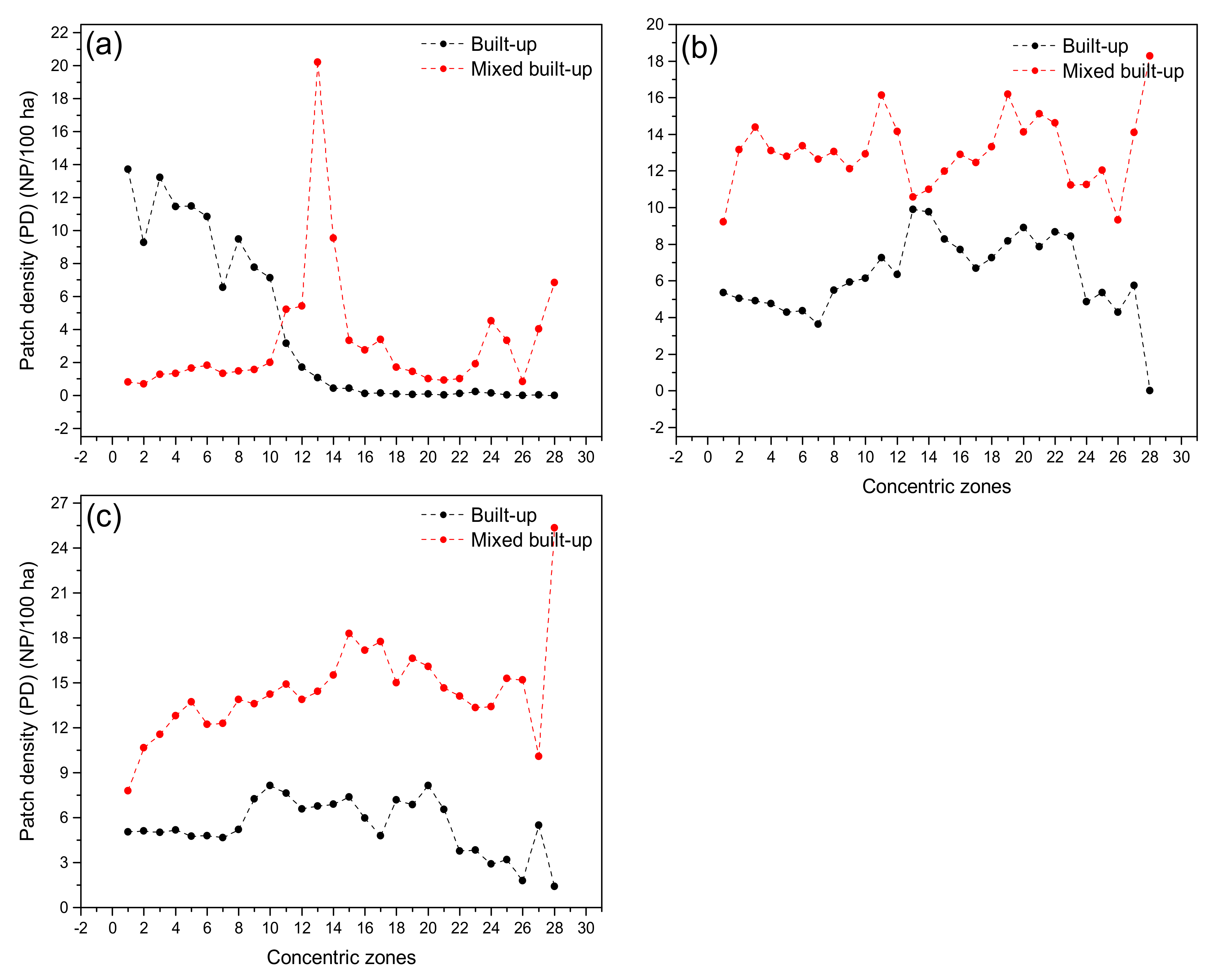
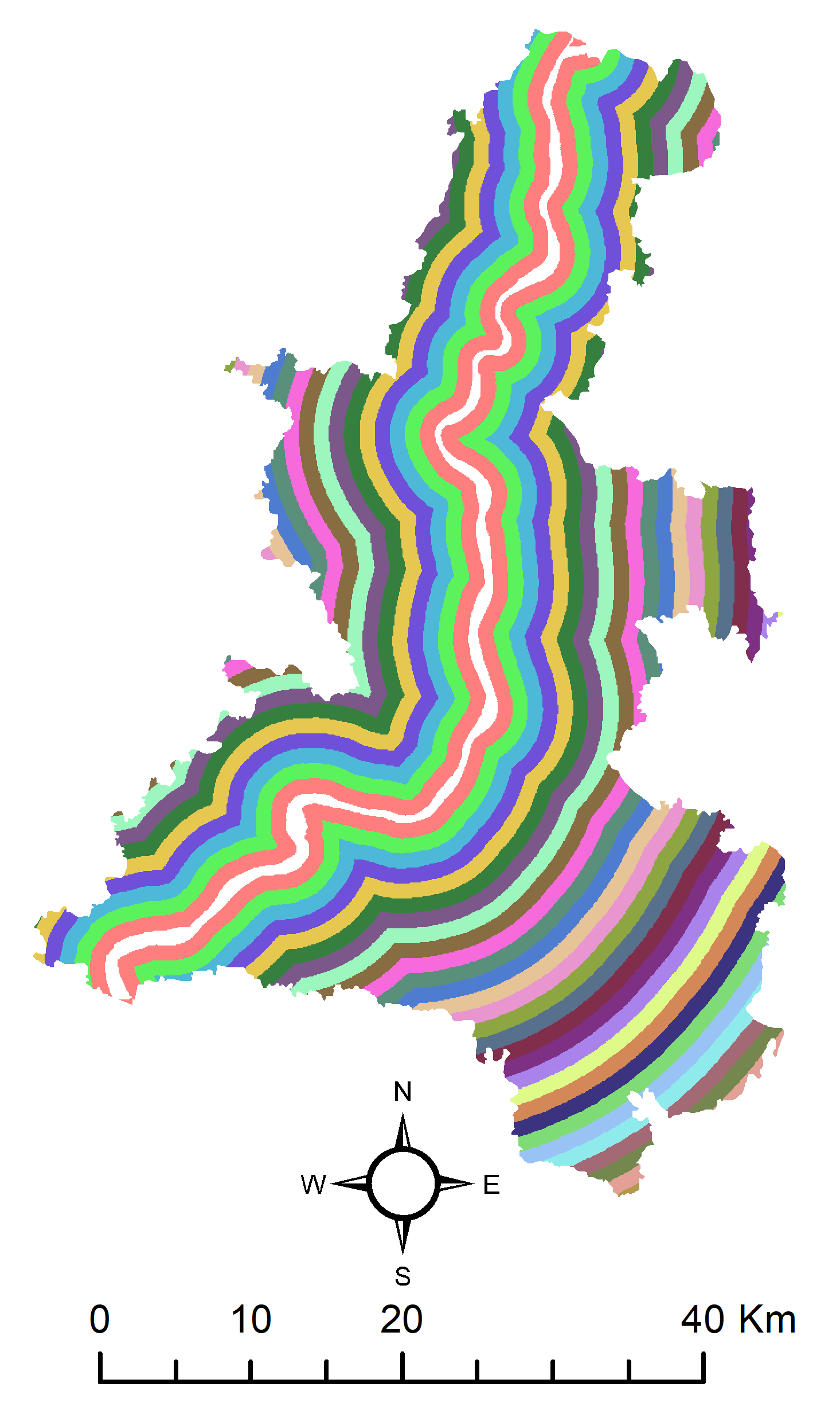
3.6. Concentric Zone Analysis

In order to investigate the changes in the spatial pattern of urban growth in KMA from center parts towards the periphery irrespective of rural-urban distinction, a concentric zone approach was devised and used. In this zoning approach, a number of sequential concentric zones of 1 km width each were demarcated around the river Hooghly to the end of the boundary of the metropolitan area (Appendix F). The results of some selected landscape metrics were computed for each of the concentric zones for 1996, 2006, and 2016.
The results of PLAND using the concentric zone approach are shown in Figure 16. The PLAND of built-up reveals a consistent trend of downward change over the years from the center to the periphery. However, some irregularities were observed in the case of the mixed built-up class. For 1996, the PLAND of mixed built-up presents an asymmetrical trend with distance, characterized by a prominent peak in the middle. The peak signifies rapid built-up growth along with a transition between statutory urban and rural areas within the metropolitan area. In addition, the curve ends with an upward trend indicating a relatively higher proportion of built-up, which might have been because of large-scale KMA-ward migration. The scenarios for 2006 and 2016 show a net increase of built-up towards the periphery. The higher PLAND of mixed built-up towards the periphery explains the process of fresh, low density, dispersed, and rapid built-up development towards the periphery of the metropolitan area, popularly known as urban sprawl.
In 1996, the scenario of built-up PD displayed a net decrease towards the periphery; the PD of mixed built-up surpassed that of built-up at the 11th zone and onwards because of the presence of a large number of mixed built-up patches towards the periphery. The cases of 2006 and 2016 also highlighted that the density of mixed built-up patches was much higher as compared to the built-up PD. Moreover, in 2016, an overall upward trend in the mixed built-up curve was observed, explaining the recent rapid and fragmented built-up growth, particularly towards the periphery of the metropolitan area (Figure 17).
The concentric zone analysis of LPI for built-up and mixed built-up classes is shown in Figure 18. For all the years considered, the LPI of the built-up class showed a descending trend towards the periphery, which is a clear reflection of the fragmentation of built-up cover towards the periphery. On the other hand, the LPI of mixed built-up cover exceeded the LPI of the built-up class after a certain distance in all years. Therefore, towards the central part, i.e., within the KMA-urban, the built-up LPI exhibited a larger size, and towards the periphery, i.e., towards the KMA-rural, the LPI of mixed built-up surpassed that of the built-up class. The scenario emphasizes the process of rapid and recent fragmented built-up growth along with the peri-urban areas in KMA.
For all the years considered, the AREA_MNs showed the presence of larger size built-up patches towards the central parts, while towards the periphery, AREA_MNs were relatively very low, reflecting a progressive declining trend with distance. The mixed built-up class demonstrated a similar pattern in AREA_MN across the concentric zones from the central parts towards the periphery. In the central part, the built-up class contained patches of much larger size, while towards the periphery, both the classes were characterized by smaller patches. The results account for the presence of small and fragmented built-up patches over the peri-urban areas in KMA (Figure 19).
The arguments between aggregated and disaggregated built-up growth and compact and dispersed growth were further examined through the deployment of AI. Over the years, the concentric zones placed within the KMA-urban displayed a high AI value of the built-up class. However, the values of AI tend to drop to a large extent beyond the statutory urban areas of KMA. On the other hand, the AI of mixed built-up was characterized by a uniform pattern with spikes across the concentric zones. Within the KMA-urban, the AI values of the built-up class were much higher compared to those of mixed built-up. Over the KMA-rural, the AI values of both classes were uniform. Therefore, the central parts of KMA were characterized by compact and aggregated patterns of built-up growth, while peripheral parts within KMA-rural were characterized by the disaggregated and dispersed nature of built-up development (Figure 20).

4. Discussion

KMA has witnessed continuous built-up and mixed built-up spread over time at the cost of non-built-up land coverage. However, substantial variation was found in such growth between KMA-urban and KMA-rural. In KMA-rural, the built-up and mixed built-up grew rapidly as a result of peripheral expansion. KMA-urban was characterized by positive growth in built-up cover and negative growth in mixed built-up cover. This explains the conversion of the mixed built-up cover into the built-up cover in KMA-urban. The gain and loss dynamics resulted in the built-up class as the most persistent land cover, followed by the mixed built-up cover in KMA. Mixed built-up cover was largely being transitioned into built-up cover in KMA-urban, while in KMA-rural, all non-built-up land cover types were largely being transitioned into mixed built-up covers. Mixed built-up has been the most significant negative contributor to non-built-up covers, followed by the built-up cover. A dilemma in urban growth seems to be evident in the metropolitan area, where, on the one hand, the non-built-up land covers were being converted into mixed built-up along the periphery at a large scale as a result of urban sprawl; on the other hand, because of the processes of urban growth such as infill, expansion, and edge growth, the existing mixed built-up areas were also being converted into pure urban built-up areas over time [4,55].
The results of NP and PD showed an increasing trend in mixed built-up over KMA-rural, implying the incidence of an increase in fragmented urban growth over KMA-rural with time. KMA-urban showed a decrease in NP and PD after 2006, signifying the incidence of compact growth in KMA-urban. The built-up LPI and AREA_MN were found to be much larger in KMA-urban compared to those in KMA-rural. Over time, the LPI and AREA_MN showed an increasing trend, while non-built-up covers showed a decreasing trend in LPI and AREA_MN. The shape complexity of built-up and mixed built-up covers was quantified using Shape_MN and PAFRAC. The results indicate that over time, shape complexity in KMA-urban decreased as a result of compact urban growth, while it increased in KMA-rural as a result of rapid and haphazard built-up growth, known as urban sprawl. The core area metrics, namely TCA and CPLAND, revealed a higher growth trend in both built-up and mixed built-up covers in KMA over time. They highlighted the incidence of a considerable accumulation of new built-up development along the periphery. However, mixed built-up showed a variable trend on the same timescale over the KMA-urban and KMA-rural. The concentric zone analysis for the built-up and mixed built-up land covers employing the selected metrics, namely PD, PLNAD, LPI, AREA_MN, and AI supported the observations found in the landscape metrics analysis. In summary, they indicated that the pattern of built-up growth tended to become fragmented, sub-divided, and dispersed with movement towards the periphery. In turn, the pattern of growth became more contiguous towards the urban core [55]. The results of the H n analysis illustrated that the urban physical growth in all spatial levels in KMA was characterized by urban sprawl. However, in KMA-urban, the rate of dispersion decreased over time, evidently due to the process of built-up infill, creating more compact built-up growth. In contrast, the rate of dispersion in KMA-rural was still very high compared to KMA-urban. This implies that the rural areas lying at the periphery within KMA were sprawling at a higher pace, characterized by leapfrogging and the dispersed nature of built-up expansion [24,55].
This research adopted a zoning approach. That is, division into whole metropolitan, metropolitan-urban, and metropolitan-rural areas to analyze the metropolitan growth dynamics. Most of the existing zoning approaches analyze urban growth at different administrative levels, such as the ward or municipality level, which may not be effective in a situation such as the KMA [19,56]. This study found that the rate and pattern of urban growth were different at different spatial levels within KMA, that is, between metropolitan-rural and metropolitan-urban areas. Furthermore, as previously discussed, in a large metropolitan system such as the KMA, the urban core and rural periphery differ from one another in terms of economic structures, infrastructural development, urban amenities, local authorities, population growth, and other factors that are important in urban planning [4]. In such a large metropolitan system, the causative variables driving built-up growth in the core and periphery are distinct, and they act in different ways. Therefore, urban planning and policymaking may not be the same for an entire metropolitan system such as KMA. As a result, the current zoning technique used in this study represents the administrative and socioeconomic, as well as the demographic features of a large metropolitan system. The zoning system appears to be a reliable approach in urban growth studies and may be integrated into urban planning and policymaking processes.

5. Conclusions and Recommendations

In this article, the urban growth dynamics of KMA have been characterized and quantified by applying change detection analysis, landscape metrics, and entropy approaches with the adopted zoning approach for the period between 1996 and 2016. In the metropolitan area, the level and pattern of urban expansion have changed significantly over time. The overall findings indicate that KMA has been undergoing a typical urban sprawl. A type of duality in the urban expansion of KMA was found, where the peri-urban regions (i.e., KMA-rural) were fast developing, characterized by leapfrogging and fragmented built-up development, in contrast to the central KMA (i.e., KMA-urban), which became more compact with time.
The performance of the metrics has been tested comparatively. All of the applied metrics performed well. The H n analysis was found to be concordant with the results obtained from landscape metrics analysis. The results in the present study are supported by the spatial variation and trends in population growth in KMA, as studied by Cox [57]. Furthermore, the findings of this study support the findings of Sudhira et al. [56] and Punia and Singh [19], despite the fact that the zoning methodology, spatial metrics, and study area were different in this study. In the present research, the metrics’ results were mostly independent, and the selection of the metrics was justified. The zoning technique used appears to be a robust tool for investigating metropolitan built-up dynamics. This might provide an effective way of studying urban growth dynamics not just for KMA, but also for all metropolises in developing countries.
Rapid urbanization happens mostly at the expense of non-urban land coverage [58]. In countries like India, where urban planning and accompanying legal enforcement do not appear to be stringent, such peri-urban or peripheral regions are more prone to such transformation. Moreover, the growth of cities in developing countries occurs rapidly, often in a haphazard fashion and irrespective of direction. This unplanned growth is triggered by suburbanization and rural-urban migration. The timely long-term measurement and monitoring of built-up dynamics appear to be potentially useful to policymaking communities in understanding the process of urban dynamics in big cities. Proper understanding and long-term assessment of the pattern and processes of urban growth could provide a basis to predict future urban growth. Furthermore, this understanding and monitoring could aid in addressing the links between urban dynamics with different socioeconomic and environmental processes in order to make urban planning more effective, efficient, and sustainable in the present and in the future. On the basis of the findings of the present study, a number of policy recommendations are proposed below for achieving SDG 11.3 in the Kolkata Metropolitan Area:
  • In the KMA, urban sprawl has irreversible negative environmental impacts. The metropolitan area’s growth has been unchecked as the suburbanization rapidly engulfs the agricultural land, vegetation cover, and water bodies, mostly in the form of mixed built-up along the periphery of KMA. Moreover, such consequences are likely to be aggravated in the coming decades. Hence, this study may be regarded as an alarm for city administrators and policymakers to gain understanding in order to take the necessary actions required for sustainable land management planning, especially for the peri-urban areas, which are more vulnerable to concretization.
  • The findings of the present study indicate that the pattern and process of urban expansion vary at different levels within the KMA, that is, between KMA-urban and KMA-rural. Furthermore, within the KMA, the urban core and rural periphery differ in terms of economic structures, infrastructure development, urban amenities, local government, population growth, and other factors that are important in the urban planning process. The causal factors driving built-up development in the core and periphery in a big metropolitan such as KMA are also largely different. Therefore, in order to achieve SDG 11.3 in the KMA, urban planning and policymaking cannot be the same for the entire metropolitan system.
  • In developing countries, cities grow rapidly, often in a haphazard fashion irrespective of direction. The timely long-term assessment and modeling of built-up dynamics appear to be of value in large cities like KMA for understanding the process of urban growth dynamics and for the allocation of resources in the present and future, depending upon changing scenarios required for sustainable long-term urban planning and development.
  • This study found that the peripheral parts of the KMA, particularly towards the west, south-west, south, south-east, and east regions, were growing at a faster pace and are expected to accelerate with further concretization in the near future. Hence, it is timely for city administrators, the planning authorities, and policy-making bodies to consider peripheral residential development of townships compatible with environmental sustainability and with provision of proper and adequate urban amenities and infrastructures.
  • Urban floods and water logging are frequent phenomena in KMA. These are also consequences of the haphazard and unplanned urban growth that has happened in KMA over the decades. To avoid such problems in the future, there is a need to have a metropolitan area as well as different spatial level identification of suitable areas favoring urban development in KMA. The suitability mapping should be based on all possible local and regional factors affecting urban growth. Future residential and infrastructural development should be strictly based on suitable areas so identified.
  • In order to reduce the consequences of urban sprawl in the future, future growth should be target-based at a local and metropolitan level over time periods. Any discrepancy between actual and target growth needs to be estimated on a decadal basis in the future. Provision for urban planning should be properly integrated with target-based growth. This could promote compact urban growth and avoid leapfrogging and haphazard built-up growth in the future.

Author Contributions

Conceptualization, S.M. and S.C.; methodology, S.M. and S.C.; software, S.M. and S.C.; validation, S.M., K.M.K. and S.C.; formal analysis, S.M. and S.C.; investigation, S.M. and S.C.; resources, S.M. and S.C.; data curation, S.M. and S.C.; writing—original draft preparation, S.M. and M.S.; writing—review and editing: M.S., B.A.J., K.M.K. and R.A.; visualization, S.M., M.S., B.A.J., K.M.K. and R.A.; supervision, S.C.; project administration S.M. and S.C.; funding acquisition, B.A.J., K.M.K. and R.A. All authors have read and agreed to the published version of the manuscript.

Funding

This work was supported by the Deanship of Scientific Research at King Khalid University through the large research groups under grant number RGP. 1/372/42.

Data Availability Statement

The data that support the findings of this study are available from the corresponding author upon reasonable request.

Acknowledgments

All the authors would like to thank USGS for the satellite data and Grants-in-aid for scientific research (Kakenhi) number 21K05664.

Conflicts of Interest

The authors declare no conflict of interest.

Appendix A

Table A1. Details of the satellite images used in the present study.
Satellite ImageAcquisition DatePath & RowLand Cloud Coverage (%)Reference System
Landsat TM16 February 1996138 & 44NilUTM (Zone 45N) & WGS 84
Landsat TM16 February 1996138 & 45NilUTM (Zone 45N) & WGS 84
Landsat TM12 December 1996138 & 44≤2UTM (Zone 45N) & WGS 84
Landsat TM12 December 1996138 & 45≤2UTM (Zone 45N) & WGS 84
Landsat OLI7 December 1996138 & 44<1UTM (Zone 45N) & WGS 84

Appendix B

Table A2. The LULC classes and their corresponding description as adopted in the current study.
ClassesDefinition and Description
Built-up areasAll impervious structures (e.g., asphalt, concrete, etc.) typically residential, commercial and industrial areas, village settlements, and transport infrastructures.
Mixed built-upBuilt-up cover mixed with vegetation and other no built-up cover.
Water bodiesRiver, canals, ponds, reservoirs, wetlands, lakes, marshy land, and other permanent water bodies.
VegetationTrees, mixed forest, shrub, and semi-natural forests.
Agricultural landCrop or cultivated land and pasture, playground, parks, lawn, dumping station, grassland, and other urban recreational areas.
Bare landAll types of fallow or barren lands such as open space, abandoned and unirrigated areas, bare exposed rocks and soils, transitional areas, salt flats, sandy areas, etc.

Appendix C

Figure A1. The SVM generated classified LULC maps of KMA for the selected years: (a) 1996, (b) 2006, and (c), 2016.
Remotesensing 13 04423 g0a1

Appendix D

Table A3. Error matrix relating to accuracy assessment of the classified LULC map of 1996.
Classified dataReference Data
Classes *123456Row TotalUA (%)
159000526689.39
208720409393.55
300535046285.48
400356236487.50
532005716390.48
600122475290.38
Column total628959637057400
PA (%)95.1697.7589.8388.8981.4382.46
OA = 89.75%
Kappa = 0.8790
* 1 = Water bodies, 2 = Vegetation, 3 = Mixed built-up, 4 = Built-up, 5 = Agricultural land, 6 = Bare land.
Table A4. Error matrix relating to accuracy assessment of the classified LULC map of 2006.
Classified dataReference Data
Classes *123456Row TotalUA (%)
150100205394.34
206930307592.00
301583106392.06
400588029592.63
512006016493.75
600151435086.00
Column total517367966746400
PA (%)98.0494.5286.5791.6789.5593.48
OA = 92.00%
Kappa = 0.9046
* 1 = Water bodies, 2 = Vegetation, 3 = Mixed built-up, 4 = Built-up, 5 = Agricultural land, 6 = Bare land.
Table A5. Error matrix relating to accuracy assessment of the classified LULC map of 2016.
Classified dataReference Data
Classes *123456Row TotalUA (%)
154000105598.18
205110205494.44
300623006595.38
40031121211894.92
525004835882.76
600042445088.00
Column total5656661195449400
PA (%)96.4391.0793.9494.1288.8989.80
OA = 92.75%
Kappa = 0.9124
* 1 = Water bodies, 2 = Vegetation, 3 = Mixed built-up, 4 = Built-up, 5 = Agricultural land, 6 = Bare land.

Appendix E

Table A6. Statement of class areas (CA in ha) under the different LULCs in 1996, 2006, and 2016.
LevelsYearsAreas under the LULCs (ha)
Agricultural LandBare LandBuilt-UpMixed Built-UpVegetationWater Bodies
KMA199627,423.1822,391.4627,781.6526,995.6840,090.8628,381.05
200627,782.6421,190.8641,439.8727,329.5832,273.0123,042.52
201625,121.8821,751.5654,419.8530,193.0217,273.7023,919.21
KMA-urban19966602.588453.9725,885.6215,737.8514,221.1713,313.79
20066243.488787.2435,811.9914,924.529435.789007.29
20165185.539627.3945,232.4710,978.473794.229369.36
KMA-rural199620,820.613,937.491896.0311,257.8325,869.6915,067.26
200621,539.1612,403.625627.8812,405.0622,837.2314,035.23
201619,936.3512,124.179187.3819,214.5513,479.4814,549.85

Appendix F

Figure A2. Concentric zones of 1 km width each at either side of the river Hooghly within the KMA.
Remotesensing 13 04423 g0a2

References

  1. Forman, R.T.T. Land Mosaics: The Ecology of Landscapes and Regions; Cambridge University Press: Cambridge, MA, USA, 1995. [Google Scholar]
  2. Wasserman, M. Urban sprawl. Reg. Rev. 2000, 10, 9–17. [Google Scholar]
  3. Ramachandra, T.V.; Aithal, B.H.; Sanna, D.D. Insights to urban dynamics through landscape spatial pattern analysis. Int. J. Appl. Earth Obs. Geoinf. 2012, 18, 329–343. [Google Scholar] [CrossRef]
  4. Mithun, S.; Chattopadhyay, S.; Bhatta, B. Analyzing urban dynamics of metropolitan Kolkata, India by using landscape metrics. Pap. Appl. Geogr. 2016, 2, 284–297. [Google Scholar] [CrossRef]
  5. Wilson, B.; Chakraborty, A. The environmental impacts of sprawl: Emergent themes from the past decade of planning research. Sustainability 2013, 5, 3302–3327. [Google Scholar] [CrossRef] [Green Version]
  6. Torrens, P.M.; Alberti, M. Measuring Sprawl; Centre for Advanced Spatial Analysis (UCL): London, UK, 2000. [Google Scholar]
  7. Rahman, A.; Aggarwal, S.P.; Netzband, M.; Fazal, S. Monitoring urban sprawl using remote sensing and GIS techniques of a fast growing urban centre, India. IEEE J. Sel. Top. Appl. Earth Obs. Remote Sens. 2011, 4, 56–64. [Google Scholar] [CrossRef]
  8. Pandey, A.C.; Kumar, A.; Jeyaseelan, A.T. Urban built-up area assessment of Ranchi township using Cartosat-I stereopairs satellite images. J. Indian Soc. Remote Sens. 2013, 41, 141–155. [Google Scholar] [CrossRef]
  9. Yeh, A.G.O.; Li, X. A constrained CA model for the simulation and planning of sustainable urban forms by using GIS. Environ. Plann. B Plann. Des. 2001, 28, 733–753. [Google Scholar] [CrossRef] [Green Version]
  10. Kumar, J.A.V.; Pathan, S.K.; Bhanderi, R.J. Spatio-temporal analysis for monitoring urban growth—A case study of Indore city. J. Indian Soc. Remote Sens. 2007, 35, 11–20. [Google Scholar] [CrossRef]
  11. Lata, K.M.; Rao, C.S.; Prasad, V.K.; Badarianth, K.V.S.; Rahgavasamy, V. Measuring urban sprawl: A case study of Hyderabad. GIS Dev. 2001, 5, 26–29. [Google Scholar]
  12. Bhatta, B.; Saraswati, S.; Bandyopadhyay, D. Quantifying the degree-of-freedom, degree-of-sprawl, and degree-of-goodness of urban growth from remote sensing data. Appl. Geogr. 2010, 30, 96–111. [Google Scholar] [CrossRef]
  13. Bhatta, B.; Saraswati, S.; Bandyopadhyay, D. Urban sprawl measurement from remote sensing data. Appl. Geogr. 2010, 30, 731–740. [Google Scholar] [CrossRef]
  14. McGarigal, K.; Marks, B.J. FRAGSTATS: Spatial Pattern Analysis Program for Quantifying Landscape Structure; Forest Science Department, Oregon State University: Portland, OR, USA, 1994. [Google Scholar]
  15. Herold, M.; Scepan, J.; Clarke, K.C. The use of remote sensing and landscape metrics to describe structures and changes in urban land uses. Environ. Plan. A 2002, 34, 1443–1458. [Google Scholar] [CrossRef] [Green Version]
  16. Cabral, P.; Geroyannis, H.; Gilg, J.P.; Painho, M. Analysis and Modeling of Land-Use and Land-Cover Change in Sintra-Cascais Area. In Proceedings of the 8th AGILE Conference on Geographic Information Science, Columbus, OH, USA, 26–28 May 2005; pp. 51–60. [Google Scholar]
  17. Jat, M.K.; Garg, P.K.; Khare, D. Modelling of urban growth using spatial analysis techniques: A case study of Ajmer city (India). Int. J. Remote Sens. 2008, 29, 543–567. [Google Scholar] [CrossRef]
  18. Herold, M.; Goldstein, N.C.; Clarke, K.C. The spatiotemporal form of urban growth: Measurement, analysis and modeling. Remote Sens. Environ. 2003, 86, 286–302. [Google Scholar] [CrossRef]
  19. Punia, M.; Singh, L. Entropy approach for assessment of urban growth: A case study of Jaipur, India. J. Indian Soc. Remote Sens. 2012, 40, 231–244. [Google Scholar] [CrossRef]
  20. Bhatta, B. Analysis of urban growth pattern using remote sensing and GIS: A case study of Kolkata, India. Int. J. Remote Sens. 2009, 30, 4733–4746. [Google Scholar] [CrossRef]
  21. Wang, L.; Ma, L.; Song, F.; Zuo, D. Dynamics analysis of crop-landscape of agri-grazing-ecotone in Hobq desert. Res. Agric. Mod. 2009, 30, 595–598. [Google Scholar]
  22. Avtar, R.; Aggarwal, R.; Kumar, P.; Kharrazi, A.; Kurniawan, T.A. Utilizing Geospatial Information to Implement SDGs and Monitor their Progress. Environ. Monit. Assess. 2019, 192, 35. [Google Scholar] [CrossRef] [PubMed]
  23. Mondejar, M.E.; Avtar, R.; Diaz, H.L.B.; Dubey, R.K.; Esteban, J.; Gomez-Morales, A.; Hallam, B.; Mbungu, N.T.; Okolo, C.C.; Prasad, K.A.; et al. Digitalization to achieve sustainable development goals: Steps towards a Smart Green Planet. Sci. Total Environ. 2021, 794, 148539. [Google Scholar] [CrossRef]
  24. Mithun, S.; Chattopadhyay, S. Analyzing Spatio-Temporal Growth Dynamics of Kolkata Metropolitan Area (KMA). In Proceedings of the 12th International Asian Urbanization Conference, Varanasi, India, 28–30 December 2013. [Google Scholar]
  25. Singh, A. Review article digital change detection techniques using remotely-sensed data. Int. J. Remote Sens. 1989, 10, 989–1003. [Google Scholar] [CrossRef] [Green Version]
  26. Zaki, R.; Zaki, A.; Ahmed, S. Land use and land cover changes in arid region: The case new urbanized zone, northeast Cairo, Egypt. J. Geogr. Inf. Syst. 2011, 3, 173–194. [Google Scholar] [CrossRef] [Green Version]
  27. Sahana, M.; Hong, H.; Sajjad, H. Analyzing urban spatial patterns and trend of urban growth using urban sprawl matrix: A study on Kolkata urban agglomeration, India. Sci. Total Environ. 2018, 628–629, 1557–1566. [Google Scholar] [CrossRef] [PubMed]
  28. Mitra, C.; Shepherd, J.M.; Jordan, T.R. Assessment and Dynamics of Urban Growth in the City of Kolkata. In Facets of Social Geography: International and Indian Perspectives; Ashok, K.D., Wadhwa, V., Thakur, B., Costa, F.J., Eds.; Foundation Books: Delhi, India, 2012; pp. 541–555. [Google Scholar]
  29. KMDA. KMDA Annual Report. 2008. Available online: http://www.kmdaonline.org/html/aar_2011.php (accessed on 5 December 2019).
  30. Census of India. Final Population Totals. 2011. Available online: http://censusindia.gov.in/2011census/censusinfodashboard/index.html (accessed on 10 December 2019).
  31. Landis, J.R.; Koch, G.G. An application of hierarchical Kappa-type statistics in the assessment of majority agreement among multiple observers. Biometrics 1977, 33, 159–174. [Google Scholar] [CrossRef] [Green Version]
  32. Yuan, F.; Sawaya, K.E.; Loeffelholz, B.C.; Bauer, M.E. Land cover classification and change analysis of the Twin Cities (Minnesota) Metropolitan Area by multitemporal Landsat remote sensing. Remote Sens. Environ. 2005, 98, 317–328. [Google Scholar] [CrossRef]
  33. O’Neill, R.V.; Krummel, J.R.; Gardner, R.E.A.; Sugihara, G.; Jackson, B.; DeAngelis, D.L.; Milne, B.T.; Turner, M.G.; Zygmunt, B.; Christensen, S.W.; et al. Indices of landscape pattern. Landsc. Ecol. 1988, 1, 153–162. [Google Scholar] [CrossRef]
  34. Gustafson, E.J. Quantifying landscape spatial pattern: What is the state of the art? Ecosystems 1998, 1, 143–156. [Google Scholar] [CrossRef]
  35. Geoghegan, J.; Wainger, L.A.; Bockstael, N.E. Spatial landscape indices in a hedonic framework: An ecological economics analysis using GIS. Ecol. Econ. 1997, 23, 251–264. [Google Scholar] [CrossRef]
  36. Alberti, M.; Waddell, P. An integrated urban development and ecological simulation model. Integr. Assess. 2000, 1, 215–227. [Google Scholar] [CrossRef]
  37. Parker, D.C.; Evans, T.; Meretsky, V. Measuring Emergent Properties of Agent-Based Landcover/Landuse Models using Spatial Metrics. In Proceedings of the 7th Annual Conference of the International Society for Computational Economics, New Haven, CT, USA, 28–29 June 2001. [Google Scholar]
  38. Taubenböck, H.; Esch, T.; Felbier, A.; Wiesner, M.; Roth, A.; Dech, S. Monitoring urbanization in mega cities from space. Remote Sens. Environ. 2012, 117, 162–176. [Google Scholar] [CrossRef]
  39. Zhang, Q. Spatial-Temporal Patterns of Urban Growth in Shanghai, China: Monitoring, Analysis, and Simulation. Ph.D. Thesis, School of Architecture and Built Environment, KTH Royal Institute of Technology, Stockholm, Sweden, 2009. [Google Scholar]
  40. Pham, H.M.; Yamaguchi, Y.; Bui, T.Q. A case study on the relation between city planning and urban growth using remote sensing and spatial metrics. Landsc. Urban Plan. 2011, 100, 223–230. [Google Scholar] [CrossRef]
  41. Tian, G.; Jiang, J.; Yang, Z.; Zhang, Y. The urban growth, size distribution and spatio-temporal dynamic pattern of the Yangtze River delta megalopolitan region, China. Ecol. Model. 2011, 222, 865–878. [Google Scholar] [CrossRef]
  42. Kong, F.; Yin, H.; Nakagoshi, N.; James, P. Simulating urban growth processes incorporating a potential model with spatial metrics. Ecol. Indic. 2012, 20, 82–91. [Google Scholar] [CrossRef]
  43. Lü, Y.; Feng, X.; Chen, L.; Fu, B. Scaling effects of landscape metrics: A comparison of two methods. Phys. Geogr. 2013, 34, 40–49. [Google Scholar] [CrossRef]
  44. Wu, W.; Zhao, S.; Zhu, C.; Jiang, J. A comparative study of urban expansion in Beijing, Tianjin and Shijiazhuang over the past three decades. Landsc. Urban Plan. 2015, 134, 93–106. [Google Scholar] [CrossRef]
  45. Hardin, P.J.; Jackson, M.W.; Otterstrom, S.M. Mapping, Measuring, and Modeling Urban Growth. In Geo-Spatial Technologies in Urban Environments; Jensen, R.R., Gatrell, J.D., McLean, D., Eds.; Springer: Berlin/Heidelberg, Germany, 2007; pp. 165–166. [Google Scholar]
  46. Cushman, S.A.; McGarigal, K.; Neel, M.C. Parsimony in landscape metrics: Strength, universality, and consistency. Ecol. Indic. 2008, 8, 691–770. [Google Scholar] [CrossRef]
  47. Bhatta, B. Urban Growth Analysis and Remote Sensing: A Case Study of Kolkata, India 1980–2010; Springer: Dordrecht, The Netherlands, 2012. [Google Scholar]
  48. Araya, Y.H.; Cabral, P. Analysis and modeling of urban land cover change in Setúbal and Sesimbra, Portugal. Remote Sens. 2010, 2, 1549–1563. [Google Scholar] [CrossRef] [Green Version]
  49. McGarigal, K.; Cushman, S. Comparative evaluation approaches to the study of habitat fragmentation. Ecol. Appl. 2002, 12, 335–345. [Google Scholar] [CrossRef]
  50. Li, X.; Yeh, A.G.O. Analyzing spatial restructuring of land use patterns in a fast growing region using remote sensing and GIS. Landsc. Urban Plan. 2004, 69, 335–354. [Google Scholar] [CrossRef]
  51. Thomas, R.W. Information Statistics in Geography. Concepts and Techniques in Modern Geography; The Invicta Press: Ashford Kent, UK, 1981. [Google Scholar]
  52. Yeh, A.G.O.; Li, X. Measurement and monitoring of urban sprawl in a rapidly growing region using entropy. Photogramm. Eng. Remote Sens. 2001, 67, 83–90. [Google Scholar]
  53. Smith, D.M. Patterns in Human Geography; Penguin: Harmondsworth, UK, 1975. [Google Scholar]
  54. Tsai, Y. Quantifying urban form: Compactness versus “sprawl”. Urban Stud. 2005, 42, 141–161. [Google Scholar] [CrossRef]
  55. Mithun, S. Quantifying and modeling metropolitan growth dynamics: A case study on Kolkata Metropolitan Area. Ph.D. Thesis, Indian Institute of Technology Kharagpur, Kharagpur, India, 2020. [Google Scholar]
  56. Sudhira, H.S.; Ramachandra, T.V.; Jagadish, K.S. Urban sprawl: Metrics, dynamics and modelling using GIS. Int. J. Appl. Earth Obs. Geoinf. 2004, 5, 29–39. [Google Scholar] [CrossRef]
  57. Cox, W. The Evolving Urban Form: Kolkata: 50 Mile City. 2012. Available online: http://www.newgeography.com/content/002620-the-evolving-urban-form-kolkata-50-mile-city (accessed on 10 December 2019).
  58. Rahman, M.; Avtar, R.; Yunus, A.P.; Dou, J.; Misra, P.; Takeuchi, W.; Sahu, N.; Kumar, P.; Johnson, B.A.; Dasgupta, R.; et al. Monitoring Effect of Spatial Growth on Land Surface Temperature in Dhaka. Remote Sens. 2020, 12, 1191. [Google Scholar] [CrossRef] [Green Version]
Figure 1. Study area map. (A) Location of KMA in India; (B) The adopted zoning approach in the present study [4]; (C) Historical growth of the urban agglomeration of Kolkata (source: based on NATMO special series map, Plate 14); (D) Decadal population accumulation in KMA and suburbs of KMA during 1901–2011.
Remotesensing 13 04423 g001
Figure 2. Methodological flowchart for quantifying urban growth in KMA.
Remotesensing 13 04423 g002
Figure 3. Total built-up spread and dynamics in KMA from 1996 to 2016: (ac) present spatial built-up spread over KMA for 1996, 2006, and 2016, respectively; the decadal built-up growth during 1996–2006 and 2006–2016 are portrayed by (d,e), respectively; while (f) reflects built-up spread in 1996, 2006, and 2016 over KMA altogether.
Remotesensing 13 04423 g003
Figure 4. Distribution of percentage of landscape, PLAND (%) of the six LULCs and their temporal change in 1996, 2006, and 2016 in (a) KMA, (b) KMA-urban, and (c) KMA-rural.
Remotesensing 13 04423 g004
Figure 5. Magnitude (ha) of gains and losses in the LULCs of KMA; (a) gains and losses between 1996 and 2006, (b) gains and losses between 2006 and 2016, and (c) gains and losses between 1996 and 2016.
Remotesensing 13 04423 g005
Figure 6. The spatial trend in gains and losses in the LULCs of KMA between 1996 and 2016; (a) gains, losses, and persistence in water bodies, (b) gains, losses, and persistence in vegetation, (c) gains, losses, and persistence in mixed built-up, (d) gains, losses, and persistence in built-up, (e) gains, losses, and persistence in agricultural land, and (f) gains, losses, and persistence in bare land.
Remotesensing 13 04423 g006
Figure 7. Magnitude of net change (ha) in the LULCs of KMA; (a) net change between 1996 and 2006, (b) net change between 2006 and 2016, and (c) net change between 1996 and 2016.
Remotesensing 13 04423 g007
Figure 8. Contributors and their roles to the net change (%) in the LULCs of KMA between 1996 and 2016; contributors to the net change in, (a) water bodies, (b) vegetation, (c) mixed built-up, (d) built-up, (e) agricultural land, and (f) bare land.
Remotesensing 13 04423 g008
Figure 9. Class level NP over KMA, KMA-urban, and KMA-rural depicted by (ac), in 1996, 2006, and 2016, respectively; and (df) present the temporal variation in PD of the LULCs over KMA, KMA-urban, and KMA-rural, respectively, in 1996, 2006, and 2016.
Remotesensing 13 04423 g009
Figure 10. Class level LPI and AREA_MN; (ac) show class level LPI for the LULCs over KMA, KMA-urban, and KMA-rural, respectively, in 1996, 2006, and 2016; and (df) reflects class level temporal trend in AREA_MN over KMA, KMA-urban, and KMA-rural, respectively, in 1996, 2006, and 2016.
Remotesensing 13 04423 g010
Figure 11. Class level Shape_MN and PAFRAC of built-up and mixed built-up classes; (ac) present the Shape_MN of built-up and mixed built-up class for KMA, KMA-urban, and KMA-rural, respectively, in 1996, 2006, and 2016; and (df) show the results of PAFRAC for KMA, KMA-urban, and KMA-rural, respectively, in 1996, 2006, and 2016.
Remotesensing 13 04423 g011
Figure 12. Class level CPLAND and TCA; (ac) present results of CPLAND metric for KMA, KMA-urban, and KMA-rural, respectively, in 1996, 2006, and 2016; while (df) represent CAI_MN for KMA, KMA-urban, and KMA-rural, respectively, in 1996, 2006, and 2016.
Remotesensing 13 04423 g012
Figure 13. Class level ENN_MN; (ac) present temporal dynamics of class level ENN_MN in KMA, KMA-urban, and KMA_rural, respectively, in 1996, 2006, and 2016.
Remotesensing 13 04423 g013
Figure 14. Class level MESH for the LULCs; (ac) represent MESH for KMA, KMA-urban, and KMA-rural, respectively, in 1996, 2006, and 2016.
Remotesensing 13 04423 g014
Figure 15. Class level aggregation metrics over KMA, KMA-urban, and KMA-rural with their temporal dynamics during 1996–2016; (ac) represent AI for KMA, KMA-urban, and KMA-rural, respectively, in 1996, 2006, and 2016; (df) show the temporal trend of nLSI for KMA, KMA-urban, and KMA-rural, respectively, in 1996, 2006 and 2016; (gi) depict temporal dynamics in PLADJ for KMA, KMA-urban, and KMA-rural, respectively, in 1996, 2006, and 2016; (jl) present CLUMPY for KMA, KMA-urban, and KMA-rural, respectively, in 1996, 2006, and 2016.
Remotesensing 13 04423 g015
Figure 16. Pattern of the PLAND plotted against the sequential concentric zones of 1 km width each around the river Hooghly within the KMA; the pattern of PLAND of built-up and mixed built-up for the concentric zones in (a) 1996, (b) 2006, and (c) 2016.
Remotesensing 13 04423 g016
Figure 17. Pattern of PD plotted against the sequential concentric zones of 1 km each around the river Hooghly within the KMA; the pattern of PD of built-up and mixed built-up for the concentric zones in (a) 1996, (b) 2006, and (c) 2016.
Remotesensing 13 04423 g017
Figure 18. Pattern of LPI plotted against the sequential concentric zones of 1 km each around the river Hooghly within the KMA; the pattern of LPI of built-up and mixed built-up for the concentric zones in (a) 1996, (b) 2006, and (c) 2016.
Remotesensing 13 04423 g018
Figure 19. Pattern of AREA_MN plotted against the sequential concentric zones of 1 km each around the river Hooghly within the KMA; the pattern of AREA_MN of built-up and mixed built-up for the concentric zones in (a) 1996, (b) 2006, and (c) 2016.
Remotesensing 13 04423 g019
Figure 20. Pattern of AI in the sequential concentric zones of 1 km each around the river Hooghly within the KMA; the pattern of AI of built-up and mixed built-up for the concentric zones in (a) 1996, (b) 2006, and (c) 2016.
Remotesensing 13 04423 g020
Table 1. Summary of accuracy assessment of the classified images.
YearOverall Accuracy (OA)Kappa Index
199689.75%0.879
200692.00%0.904
201692.75%0.912
Table 2. Decadal growth (%) in the LULCs over KMA, KMA-urban, and KMA-rural during 1996–2006, 2006–2016, and 1996–2016.
LevelsPeriodsLand Use Land Covers (LULCs)
Agricultural LandBare LandBuilt-UpMixed Built-UpVegetationWater Bodies
(%)(%)(%)(%)(%)(%)
KMA1996–20061.31−5.3649.161.24−19.5−18.81
2006–2016−9.582.6531.3210.48−46.483.8
1996–2016−8.39−2.8695.8811.84−56.91−15.72
KMA-urban1996–2006−5.443.9438.35−5.17−33.65−32.35
2006–2016−16.949.5626.31−26.44−59.794.02
1996–2016−21.4613.8874.74−30.24−73.32−29.63
KMA-rural1996–20063.45−11.01196.8210.19−11.72−6.85
2006–2016−7.44−2.2563.2554.89−40.983.67
1996–2016−4.25−13.01384.5670.68−47.89−3.43
Table 3. Results of H n analysis and the corresponding Log(n) values for built-up and mixed built-up classes over KMA, KMA-urban, and KMA-rural in 1996, 2006, and 2016.
YearsLevelsShannon’s Entropy ( H n ) Log(n)
Built-UpMixed Built-UpAll Built-UpBuilt-UpMixed Built-UpAll Built-Up
1996KMA1.151.631.481.891.891.89
KMA-urban1.041.381.241.631.631.63
KMA-rural1.211.291.301.531.531.53
2006KMA1.351.591.601.891.891.89
KMA-urban1.191.371.301.631.631.63
KMA-rural1.311.301.201.531.531.53
2016KMA1.451.631.611.891.891.89
KMA-urban1.291.381.361.631.631.63
KMA-rural1.351.341.311.531.531.53
Publisher’s Note: MDPI stays neutral with regard to jurisdictional claims in published maps and institutional affiliations.

