Abstract
Subfootprint variability (SFV) is variability at a spatial scale smaller than the footprint of a satellite, and it cannot be resolved by satellite observations. It is important to quantify and understand, as it contributes to the error budget for satellite data. The purpose of this study was to estimate the SFV for sea surface salinity (SSS) satellite observations. This was performed by using a high-resolution numerical model, a 1/48° version of the MITgcm simulation, from which one year of output has recently become available. SFV, defined as the weighted standard deviation of SSS within the satellite footprint, was computed from the model for a 2° × 2° grid of points for the one model year. We present maps of median SFV for 40 and 100 km footprint size, display histograms of its distribution for a range of footprint sizes and quantify its seasonality. At a 100 km (40 km) footprint size, SFV has a mode of 0.06 (0.04). It is found to vary strongly by location and season. It has larger values in western-boundary and eastern-equatorial regions, as well as in a few other areas. SFV has strong variability throughout the year, with the largest values generally being in the fall season. We also quantified the representation error, the degree of mismatch between random samples within a footprint and the footprint average. Our estimates of SFV and representation error can be used in understanding errors in the satellite observation of SSS.
1. Introduction
Measurements of sea surface salinity (SSS) from a satellite are an important recent development that has led to an increase in our understanding of the global hydrologic cycle [1,2,3]. The retrieval of SSS from radiometric measurements of brightness temperature at L-band is a complex process [4] that has been developed over many years of effort [5]. The result is a final dataset from the NASA/SAC-D Aquarius satellite (2011–2015) and ongoing collection of high-quality data from the NASA SMAP (Soil Moisture Active Passive; 2015–present) and ESA SMOS (Soil Moisture and Ocean Salinity; 2010–present) satellites. There are a number of factors that impact the accuracy of retrieved SSS, including sea state, galactic background radiation, ionospheric corrections, thermal emission from the antenna, etc. [4,6,7]
Measurements of SSS are performed at a relatively low resolution or large footprint size, due to their use of long-wavelength radiation. The footprints are ~100 km for Aquarius [6] and ~40 km for SMAP [8]. The measurements are essentially weighted averages over the footprint for real aperture instruments, such as Aquarius and SMAP. (For SMOS, which uses an interferometric method, the nature of the image is more complicated, and the footprint size is variable.) The weighting is approximately a Gaussian function centered at the location of the estimate with a decay scale given by the footprint size [9]. Thus, the satellite estimate incorporates or averages all of the variability within the footprint [10].
The validation process for satellite data typically involves comparing satellite measurements with nearby in situ observations, mainly from Argo floats or moorings [11,12,13,14,15]. These comparisons do not take into account variability within the footprint and simply assume that a single point in situ validation measurement represents the footprint average. This variability within the footprint, or subfootprint variability (SFV), leads to representation error (RE), wherein a comparison validation measurement may not correctly represent the footprint average. RE could be a significant fraction of the total error of the satellite measurement, but is not considered when the error budget is tabulated [6,7,8]. In a sense, it should not be considered an error, as in an inaccurate measurement, at all. It is just a result of the fact that the satellite and in situ instruments make their measurements at different scales [10].
SSS SFV has been quantified in a few publications, using models and in situ observations [10,16,17,18,19,20]. Most relevant to the present investigation is that of Reference [9], who looked at SFV in a high-resolution model in two specific regions: the Western Pacific and Arabian Sea. In each, they found that SFV depends on the location and on the size of the footprint. Mid-ocean regions had typically low values of SFV, 0.05–0.1 for a 100 km footprint. Closer to the coast, or to boundary currents, the SFV could be much larger. The SFV decreased with decreasing footprint size.
Another important study is that of Vinogradova and Ponte [16], who quantified what they called “small-scale variability”, essentially the standard deviation inside 1° × 1° boxes, within the 1/12° resolution version of the Hybrid Coordinate Ocean Model (HYCOM). They published global maps of small-scale variability, showing that it is larger near the coast; within river plumes; and near major frontal zones, such as the Antarctic Circumpolar Current, Gulf Stream and Brazil–Malvinas Confluence. They showed a distribution of the values for the globe, with a mode at 0.05.
The work of References [10,19] has made it clear that SFV is a function of footprint size, location and season. Each of these studies examined SFV time series at a pair of locations, using in situ observations: one location in the evaporation-dominated high SSS region of the Subtropical North Atlantic and the other in the precipitation-dominated low SSS region of the Eastern Tropical North Pacific. In both locations, SFV exhibited strong seasonal variability. SFV was least in January–April (February–May) at the North Atlantic (Eastern Tropical North Pacific) location. Median values of SFV changed by a factor of 2 between low- and high-SFV seasons. High SFV coincided with heavy rainfall at the North Pacific site, but not exactly at the North Atlantic site. Reference [19] found that SFV increases as a function of footprint size in each location, but there is a larger dependence on scale at the North Atlantic site. The dependence on scale itself is a function of season. Both studies relied mainly on in situ data, but they also used a regional high-resolution model based on the Regional Ocean Modeling System (ROMS; [21,22]) to obtain values of SFV. This is a different model from the one we use here, but at a similar spatial resolution (~3 km). The model generally agreed with the in situ results at the North Atlantic site, but not as much at the North Pacific one. This suggests that using a high-resolution model to determine SFV is useful in many locations, especially those without persistent heavy seasonal rainfall and where SSS variability is mainly generated by internal ocean dynamics.
In this study, we quantified global SSS SFV by using a high-resolution model that has recently become available; this model is different from the ones used by References [10,19] and has four times the linear resolution as the one used by Reference [16]. We look at different footprint sizes, do Gaussian weighting for computing SFV instead of a simple box standard deviation and examine the seasonality of SFV. In addition, we examine RE. This is different from SFV [20], as we described below, and better quantifies the sampling error that is expected in the satellite measurement of SSS. Looking at SFV and RE for different footprint sizes can help in the design of potential future SSS satellite missions by informing the details of the expected error budget.
2. Data and Methods
The model we used is the same as that of Reference [23]. It is the MITgcm with a latitude–longitude polar cap (LLC) numerical grid. Reference [24] gave a lengthy description of the specifics of the model (see also References [25,26,27]).
We make brief use of monthly rainfall data from the Integrated Multi-satellitE Retrievals for GPM (IMERG). See the Data Availability Statement for access information.
2.1. The Global Model
The model is divided into 13 square tiles with 4320 grid points on each side and is thus termed “LLC4320”. The nominal horizontal grid spacing is 1/48° (~2 km at mid-latitude) with 90 vertical levels in z-coordinates (1 m vertical resolution near the surface). The effective horizontal resolution is 8 km (Rocha et al. 2016). Because of this somewhat limited resolution of the model, we cannot make any conclusions about SFV for scales smaller than that. However, Reference [28], using saildrone data from the Arctic, computed spectra of SSS variability between 1 and 10 km and found that they matched those of the LLC4320. On the basis of this one study, we think that the limited resolution of the model did not have a large impact on our results. The period of the simulation spans 13 September 2011 to 15 November 2012. However, we only used 1 November 2011 to 31 October 2012 to make a complete year. SSS is saved at hourly intervals (the model time step is smaller than that). The model output is available from 70°S to 57°N. It is forced at the surface with six-hourly surface atmospheric fields from the 0.14° European Centre for Medium-Range Weather Forecasting (ECMWF) atmospheric operational model analysis [24].
2.2. Subfootprint Variability
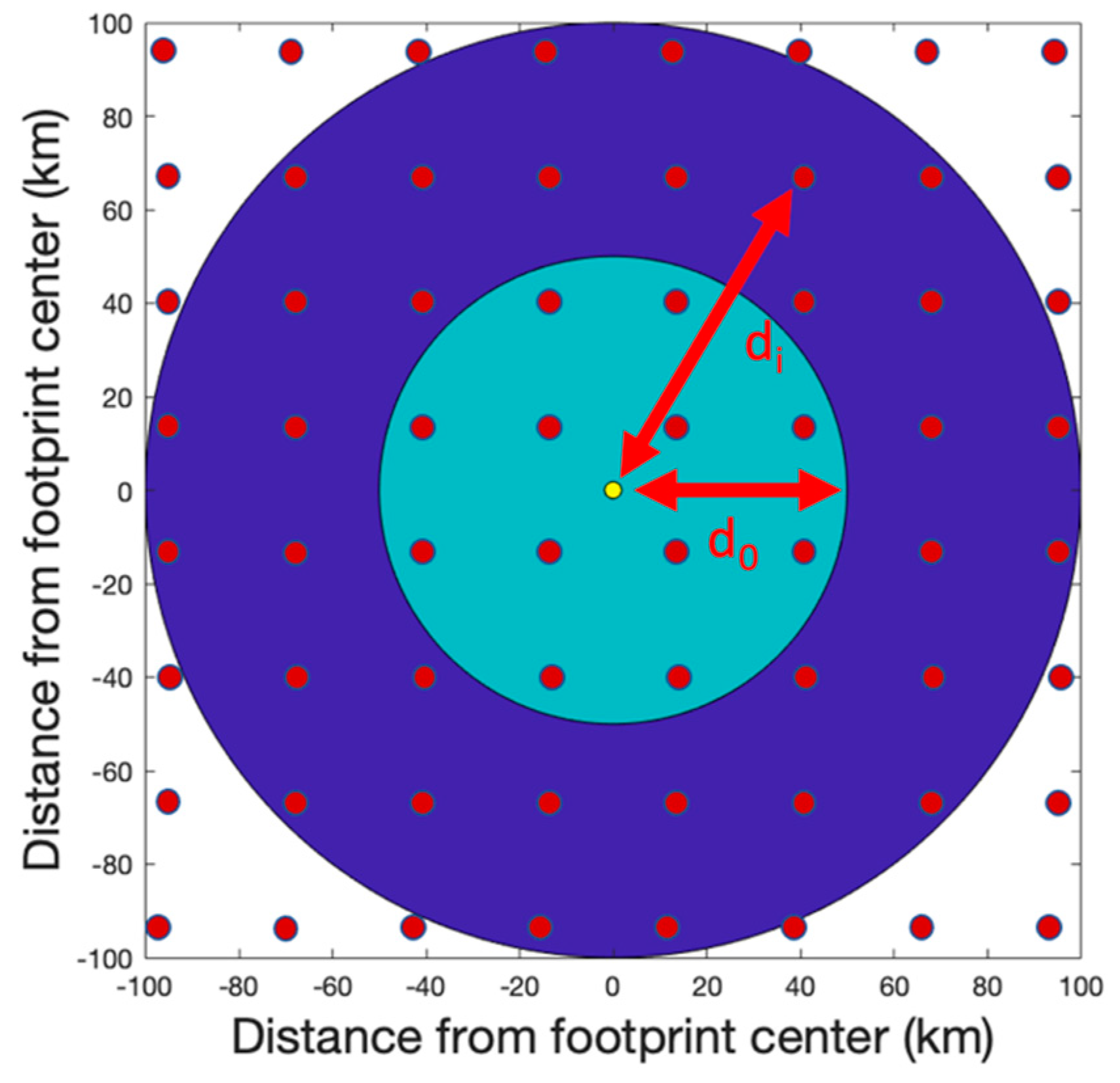
We computed SFV from the model on a 2° × 2° evaluation grid. As the model has such a high resolution, working with it is computationally challenging, and this was the smallest evaluation grid that was feasible with available computer resources. Figure 1 illustrates how we computed the SFV at each evaluation grid point (the yellow dot) from the surrounding model grid (the red circles). In this case, the footprint size is 100 km, and so the radius of the footprint is d0 = 50 km (d0 = 20 km for SMAP); di is the distance from the evaluation grid point to a model grid point. We used model grid points that were within a distance 2d0 of each evaluation grid point, the dark and light blue areas in Figure 1. In real satellite retrieval, the light blue area contains 50% of the information used to formulate the estimate, the dark blue area contains 44% and the area outside the dark blue contains 6%. (These values are taken from the weighting function discussed below.) In our computation using the model, the outside region was ignored. We computed SFV, σ, as a weighted standard deviation as follows:
where C is the set of all model grid points within a radius 2d0 of the evaluation grid point, the evaluation area, i.e., the red dots within the dark and light blue areas of Figure 1. Si is the values of salinity at each of these points. is the weighted average over the evaluation area, as described below. The wi refers to the weights assigned to each model grid point for each different evaluation grid point,
so that the values of the wi are 0.5 at a distance equal to d0 and 0.94 at a distance of 2d0. Using this method, we formed hourly time series of SFV at each evaluation grid point for the model year. We found SFV to be highly seasonal in many places [19], so we made monthly maps, some of which we present in this paper and more in the Supplementary Materials. A quantity we report is the median SFV at each evaluation grid point over some time period (e.g., one month), which is called σ50 hereafter.

Figure 1.
Schematic illustrating the relationship of the evaluation point (yellow circle), footprint size (2d0 = 100 km in this case, illustrating the situation for Aquarius) and model grid (red circles). C in Equation (1) corresponds to the set of all model grid points within the dark and light blue regions in this figure. Model grid points outside of this region were not used in estimating the SFV. The light blue region is the footprint for which weights, wi, are greater than 0.5. This figure is for illustration. For the model used in this study, the grid points would be much denser than depicted. This figure is taken from Reference [23].
We also computed an estimate of RE at each evaluation grid point. This was performed by first taking the weighted mean of SSS over the footprint:
We took a single random SSS value from the model somewhere within the footprint and subtracted that from the mean to form a time series of differences at each evaluation grid point. The RE is computed as the RMS of these differences. This process of computing the RE is meant to mimic the use of Argo float data for validation of satellite SSS.
3. Results
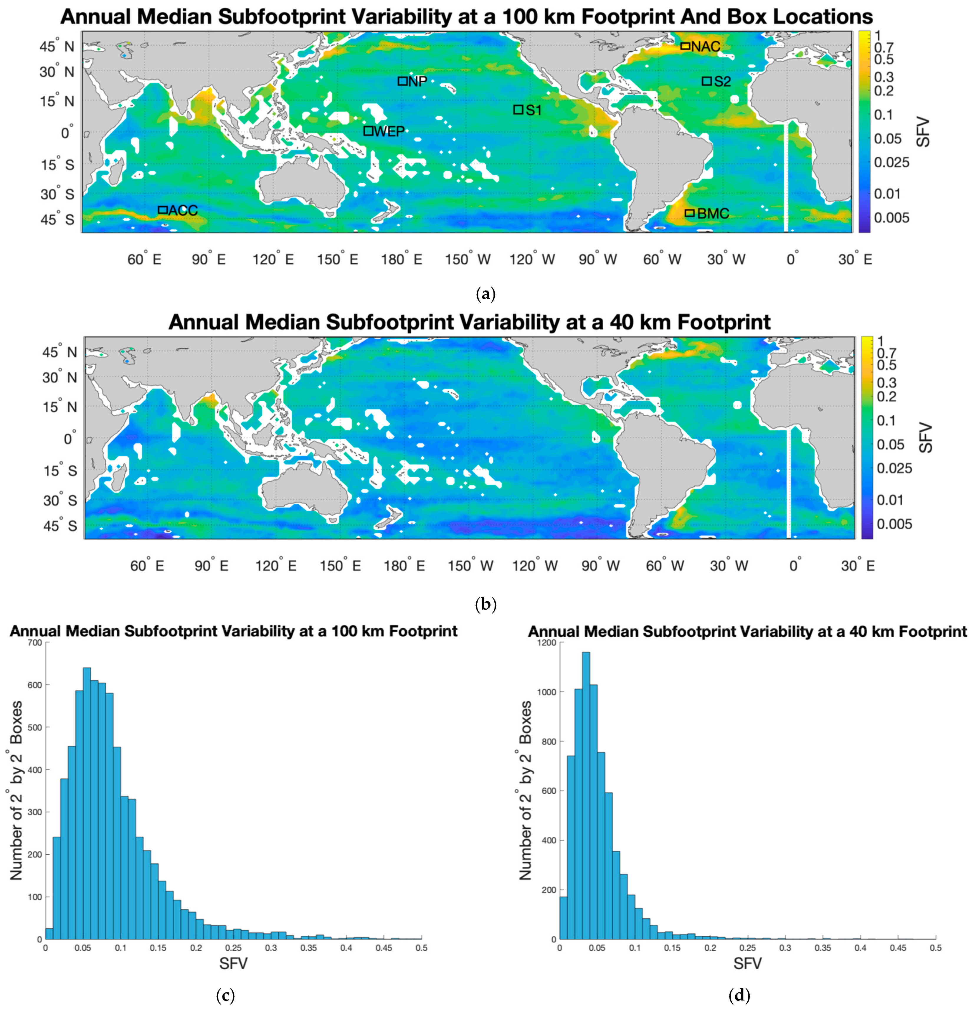
The global distribution of annual σ50 for 100 km footprint (Figure 2a) shows the size of it, and where it is relatively large or small. SFV is large near the western boundary currents, such as the Gulf Stream and North Atlantic Current, the Kuroshio Extension and the Brazil–Malvinas Confluence. The Antarctic front in the South Indian Ocean has a narrow strip of large SFV surrounded by areas of very low SFV. Parts of the tropics have large SFV, the Eastern Pacific Fresh pool and the Tropical Atlantic. The Bay of Bengal is another area with large SFV. SFV is especially small in the far Eastern South Pacific along about 45°S, in the Gulf of Alaska and in the Eastern North Atlantic. SFV is lower in the open ocean away from frontal zones, generally less than 0.1, as also shown by Reference [9] for a couple of limited regions. One area where the SFV is smaller than expected is near the Amazon outflow in the Western Tropical North Atlantic. This area has a large amount of small-scale variability in the map of Reference [16], but not here. This may be due to the use of climatological river discharge in the MITgcm [29] rather than the actual measured value. The results at a 40 km footprint size (Figure 2b) are similar to the 100 km results, but with smaller values. The Brazil–Malvinas, Gulf Stream and Bay of Bengal regions stand out in this display. Notable low SFV regions are south of the equator in the Central Pacific, along the equator in the Western Equatorial Indian and in the far South Atlantic.
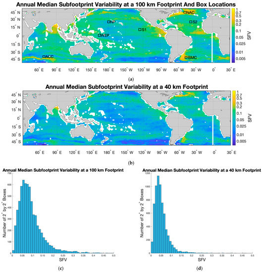
Figure 2.
(a) Median SSS SFV, i.e., σ50, for a 100 km footprint for the whole year. Unitless color scale is at right, with the colors scaling as the base 10 logarithm of the SFV. Boxes with labels in various locations are keys to the curves shown in Figure 4. The boxes are 4° × 4° in size, with SFV values averaged within the boxes. (b) Same for 40 km, but with no boxes. (c,d) Display the same median SFV median values as histograms which count the number of 2° × 2° boxes with the given SFV. The total number of boxes in both figures is 10,440. Note different y-axis limits in panels (c,d). Note that the mid-ocean blank spaces in panels (a,b) are due to small islands within the 2° × 2° boxes.
The distributions of annual σ50 (Figure 2c,d) indicate the magnitude of SFV more precisely than the maps. At 100 km, the mode is 0.06, but the distribution contains high outlier values as high as 0.5. The distribution for 40 km is lower as one would expect. The mode is a little smaller, 0.04, but more strongly peaked and with far fewer high outliers.
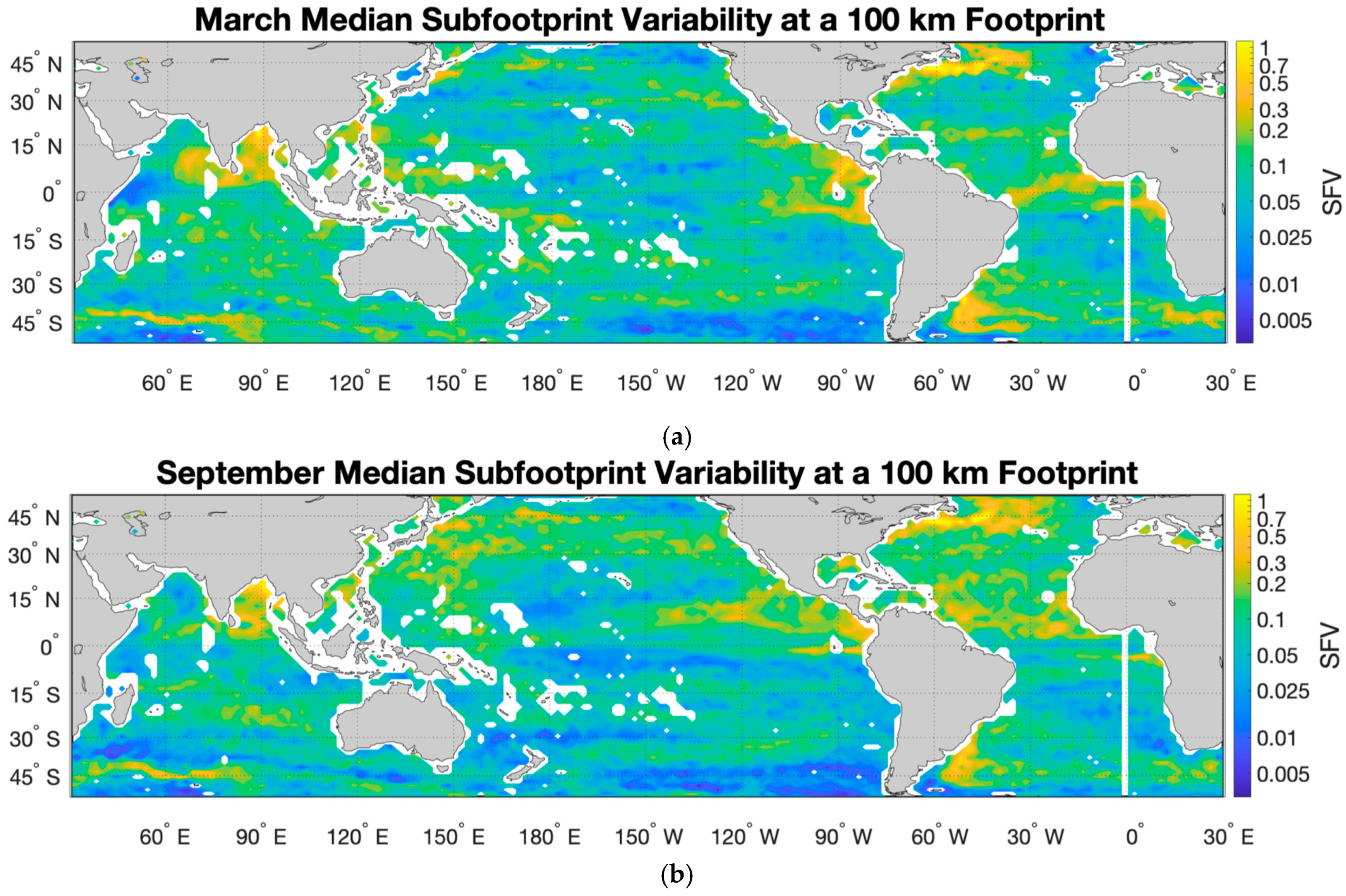
We present σ50 for a 100 km footprint for two different months, March and September (Figure 3). These months were chosen because, as is shown later, they tend to the have the largest or smallest values of SFV during the course of the year and show the most contrast. (We have included more months of maps, plus maps for 40 km footprint, in the Supplementary Materials Tables S1 and S2.)

Figure 3.
Median SSS SFV, i.e., σ50, for a 100 km footprint for the months of (a) March and (b) September. Unitless color scale is on the right, with the colors scaling with the base 10 logarithm of the SFV.
There is seasonality apparent in the maps of Figure 3 and those at 40 km (Supplementary Materials Table S2). The fall hemisphere has a larger SFV in general. Compare, for example, the northern hemisphere in the fall (Figure 3b) with the northern hemisphere in the spring (Figure 3a). In the figure, large areas of the North Atlantic and North Pacific show yellow colors in the fall, but blue and green in the spring. The same pattern holds for the southern hemisphere in the fall (Figure 3a) vs. the spring (Figure 3b), though it appears that the degree of seasonality is smaller in the southern hemisphere. The seasonality of the SFV agrees with prior findings in a couple of limited regions [10,19]. It is apparent that the northern hemisphere tends to have a larger SFV than the southern, even in the same season. Compare Figure 3a’s northern hemisphere with Figure 3b’s southern hemisphere, especially in the Pacific basin. Both are spring seasons, but the northern hemisphere has generally larger values. In addition, note that the global distribution of SFV does not resemble that of the magnitude of global precipitation (for example, see Reference [30], their Figure 4 middle). This suggests that the amount of SFV in most parts of the ocean may not be mainly due to the total amount of rainfall, but perhaps some other measure.
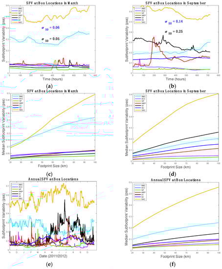
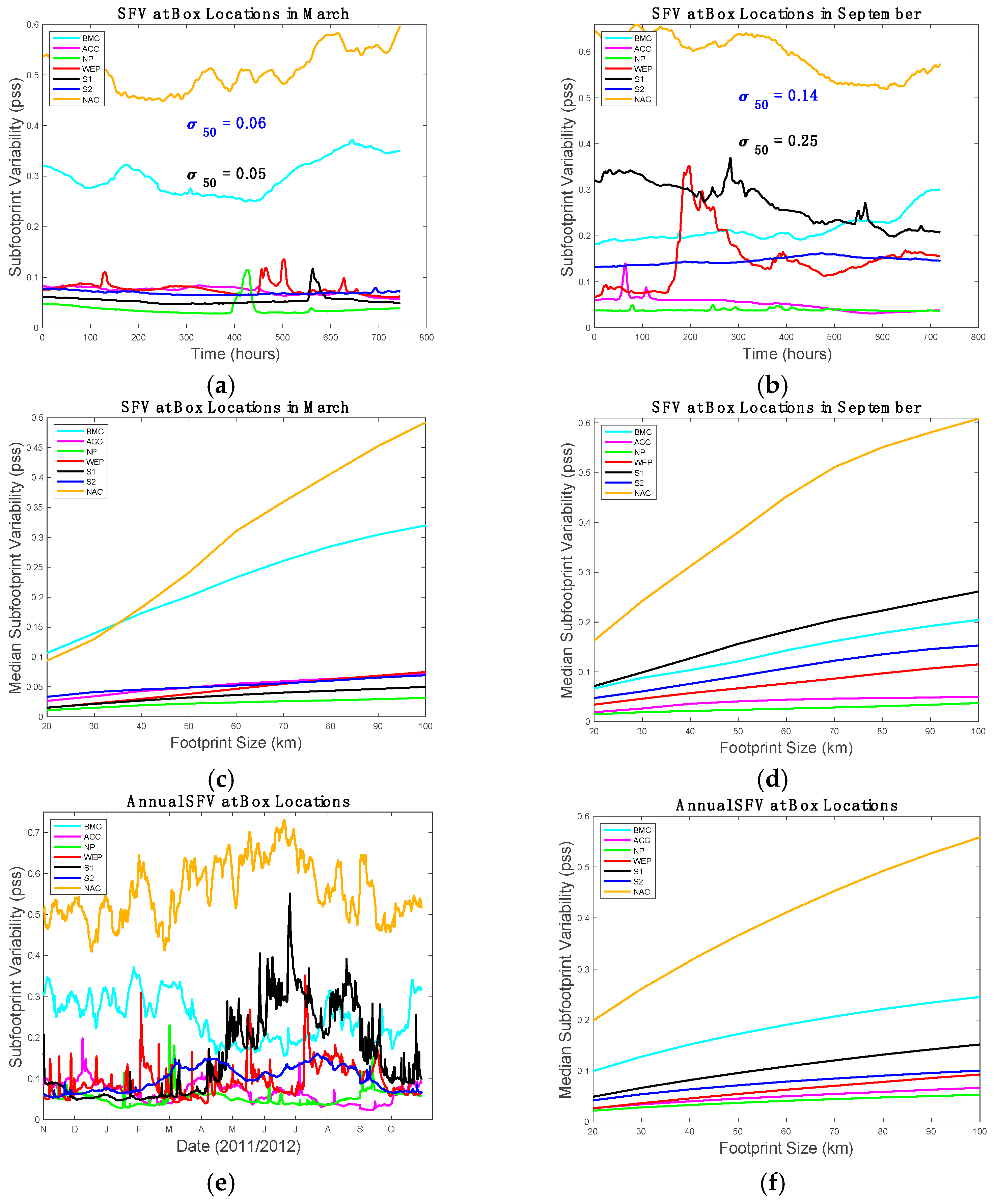
Figure 4.
(a) SFV for the month of March for 100 km footprint for the locations shown in Figure 2a. The x-axis is in hours starting on 1 March. The legend keys the line color to the box labels as described in the text and shown in Figure 2a. Median values for the SPURS-1 (“S1”) and SPURS-2 (“S2”) over the month are indicated in black and blue fonts, respectively. (b) Same as panel (a), but for September. (c) Median SFV for each location as a function of footprint size for March and (d) September, with the same curve labels as in panel (a). (e) Same as panel (a), but for the full year. (f) Same as panel (c), but for the full year. Note the variations in vertical axis limits between panels.
To see what the SFV looks like more specifically, we examined a few examples of records in boreal fall (Figure 4b) and spring (Figure 4a). The SPURS-1 (Salinity Processes in the Upper-Ocean Regional Studies—1; [31]) site in the Subtropical North Atlantic (curve “S1”) has a clear contrast between fall and spring with median value over September and March of 0.14 and 0.06 respectively. These values are similar to those computed by Reference [10] from in situ observations and a high-resolution model. At the SPURS-2 [32] site in the Tropical North Pacific (“S2”), the contrast is even larger, with median values of 0.25 and 0.05 for the fall and spring. The spring values are similar to those of Reference [19], but the fall values given here are lower. The fall record has a couple of episodic events, possibly associated with rain or the approach of the North Equatorial Countercurrent front [33]. SFV is larger in the SPURS-2 box than the SPURS-1 box in the fall, but it is comparable in the spring. Some other sites also show the same seasonality, such as the site in the Brazil–Malvinas Confluence (“BMC”) and North Atlantic current region (“NAC”). The Western Equatorial Pacific site (“WEP”) is larger in September than March. It appears that some kind of front passes by this site early in September. The mid-North Pacific (“NP”) and South Indian (“ACC”) sites have low SFV and little seasonal variation. The mid-North Pacific site has one short higher SFV event in mid-March.
The seasonality is shown more concretely by looking at records for the entire year (Figure 4e). In the northern hemisphere, the Northern North Atlantic and SPURS-1 and SPURS-2 regions have elevated SFV during the boreal fall season. The seasonal contrast is especially large in the SPURS-2 region. In the southern hemisphere, the Brazil–Malvinas Confluence region also has a strong seasonal contrast. There is a similar but less prominent seasonal contrast at the South Indian site, with minimum in austral spring. The North Pacific and Western Equatorial Pacific sites do not appear to have systematic seasonal variability.
SFV varies as a function of footprint size on an annual basis (Figure 4f), but how much it varies depends on season and location. There is a stronger dependence on footprint size in the fall than in the spring (Figure 4c,d).
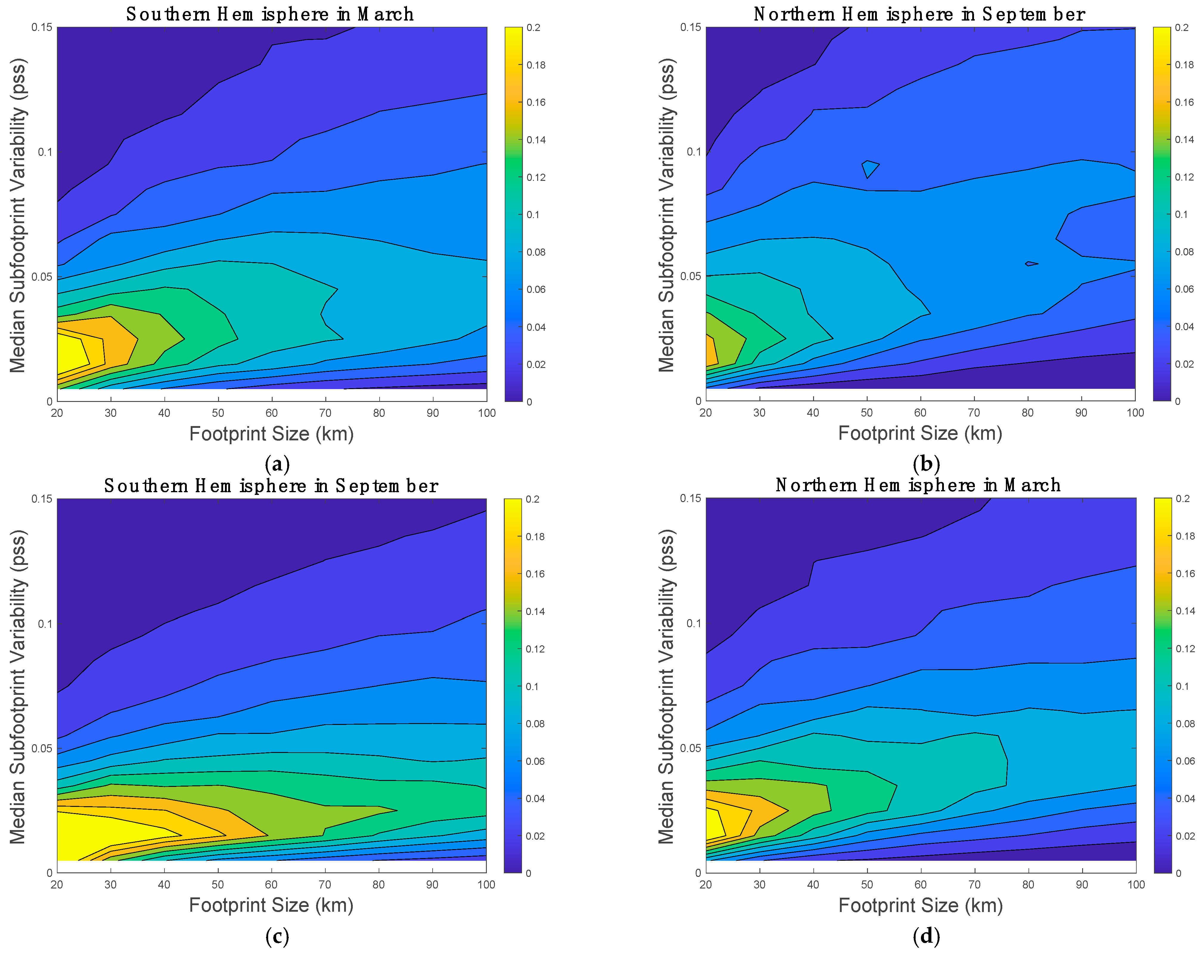
The values of SFV can be divided by hemisphere and season to show the contrast between them and get a sense of the amount of variability and distribution of SFV, as shown in Figure 5. In that figure, the more yellow the color gets, the larger the area where SFV takes on that value. In the fall season (top row) the distribution of SFV in the southern hemisphere is strongly peaked at about 0.02 for 20 km footprint, increasing to about 0.04 for 100 km footprint. The northern hemisphere is also peaked at 0.02 for 20 km footprint. It increases more, though, to 0.06–0.07 at 100 km, and has more spread in the distribution at all footprint sizes. Thus, in the fall, the northern hemisphere is less strongly peaked, and has larger outlier values. The spring season (bottom row) is similar. The southern hemisphere is strongly peaked at low values, whereas the northern hemisphere has more outliers, especially at large footprint size. Comparing the fall and spring seasons, the top and bottom rows, the fall season tends to have larger values than spring, and more especially high outliers.
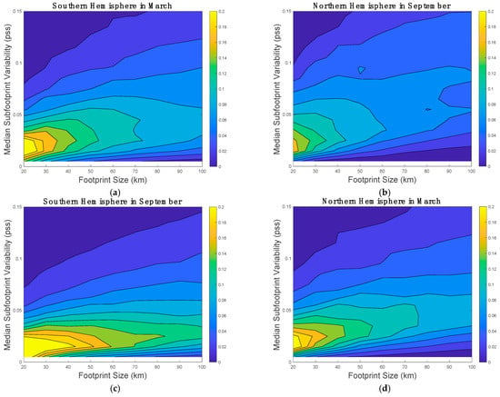
Figure 5.
Distributions of SFV as a function of footprint size broken out by hemisphere and season. For example, the values for 100 km are determined by taking a histogram of the data displayed in Figure 3a. Note that these are normalized histograms, so the values displayed do not depend on the relative areas of the southern and northern hemisphere oceans. Left column is the southern hemisphere, and right is northern. Top row is the fall season, and bottom is spring. (a) Southern hemisphere in March. (b) Northern hemisphere in September. (c) Southern hemisphere in September. (d) Northern hemisphere in March.
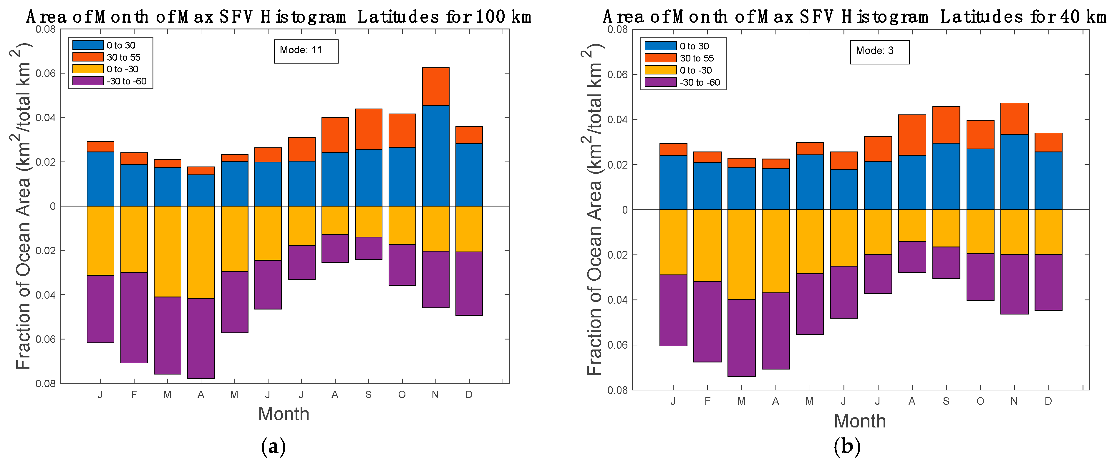
SFV has a large seasonal cycle in many places. The degree of seasonality can be examined by looking at the area where SSS is maximum by month and latitude (Figure 6). For the northern hemisphere, the month where most of the area has the maximum SFV is in the fall: November for 100 km footprint, September and November for 40 km. The southern hemisphere has similar characteristics, with the largest area having maximum SFV in February–April, i.e., fall. The area of minimum SFV (not shown for brevity) has the exact opposite phase, with most of the area being the minimum in February (August–October) for the northern (southern) hemisphere. Breaking this pattern down by latitude, we see that there appears to be relatively little seasonal variation in the northern hemisphere equatorward of 30° N (blue bars), but stronger seasonality poleward of there (red bars). In the southern hemisphere, the pattern is different. The area equatorward of 30° S does have a strong seasonal cycle, as does the area poleward of there. There is a larger area with high SFV, globally speaking, in the fall and spring seasons than in summer and winter. The global SFV is smallest in boreal summer, July and August, and largest in boreal fall (November for 100 km footprint) or austral fall (March for 40 km footprint).
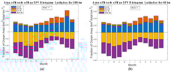
Figure 6.
Distribution of SFV evaluation grid points (e.g., yellow circle in Figure 1) by month. (a) At each grid point, the month is found where that grid point is at its maximum SFV. The normalized area (area of the 2° × 2° boxes analyzed divided by the total area of the ocean) is then summed for a given month for 100 km footprint. Yellow and purple bars are southern hemisphere, 0 to 30° S and 30° S to 60° S, respectively, increasing downward. Blue and red bars are northern, 0 to 30° N and 30° N to 55° N, respectively. The box shows the mode, or month with the most locations—November in this case. (b) Same but for 40 km footprint.
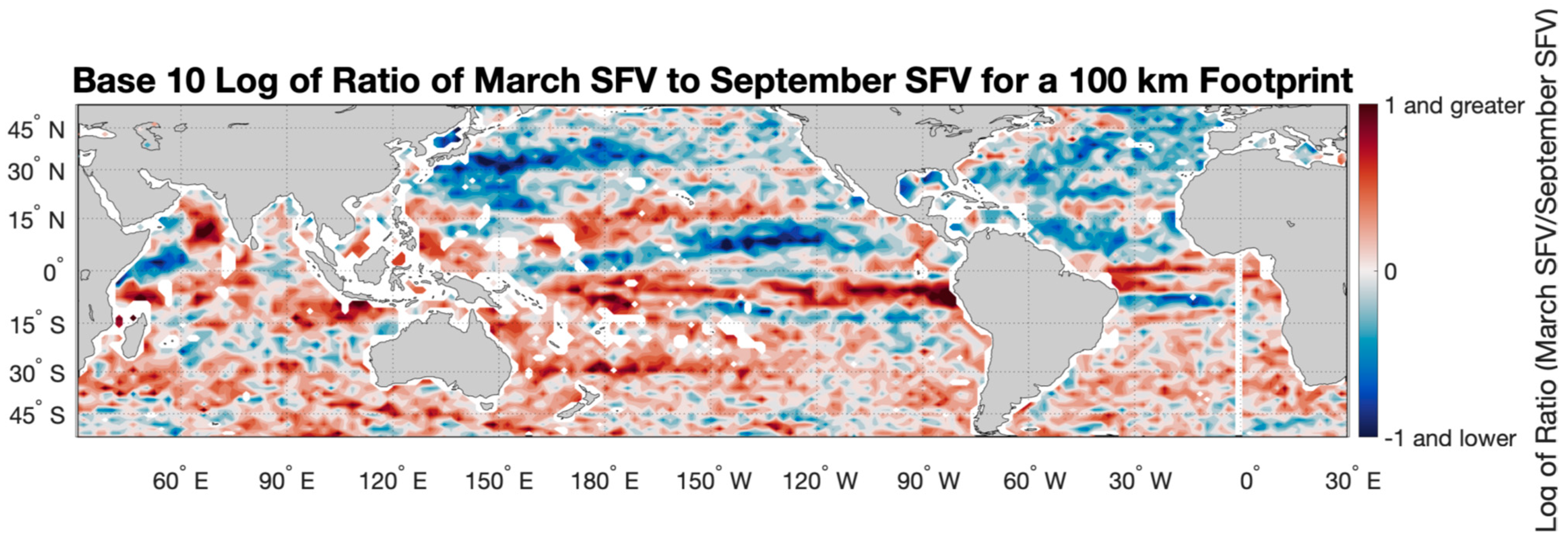
Another view of the seasonality of SFV is given in Figure 7, which shows the contrast between the fall and spring seasons and between hemispheres. The SFV is larger in September throughout much of the Central North Atlantic and North Pacific, and it is larger in March throughout the southern hemisphere. There are bands near the equator, where the ratio is either very large or very small. Along the equator itself, in all the ocean basins, the March values are larger. In the Pacific, along about 10°N, is a blue band where the September values are larger. Another red band spans the Pacific near 15°N. This set of bands is likely due the seasonal migration of the intertropical convergence zone and the associated North Equatorial Countercurrent front [33,34]. A similar set of bands is seen in the Atlantic. The Indian basin is different, with the March values larger everywhere except a small area off the Horn of Africa. The ratio is especially large in the Arabian Sea and south of the equator in the Eastern Indian Ocean.
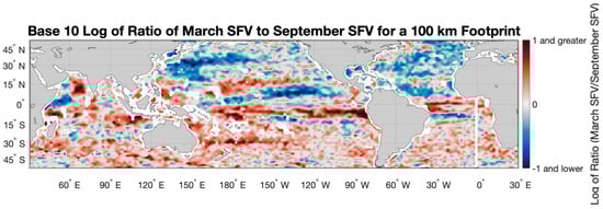
Figure 7.
Log10 of the ratio of median SFV in March to the median SFV in September for a 100 km footprint. Color scale is on the right.
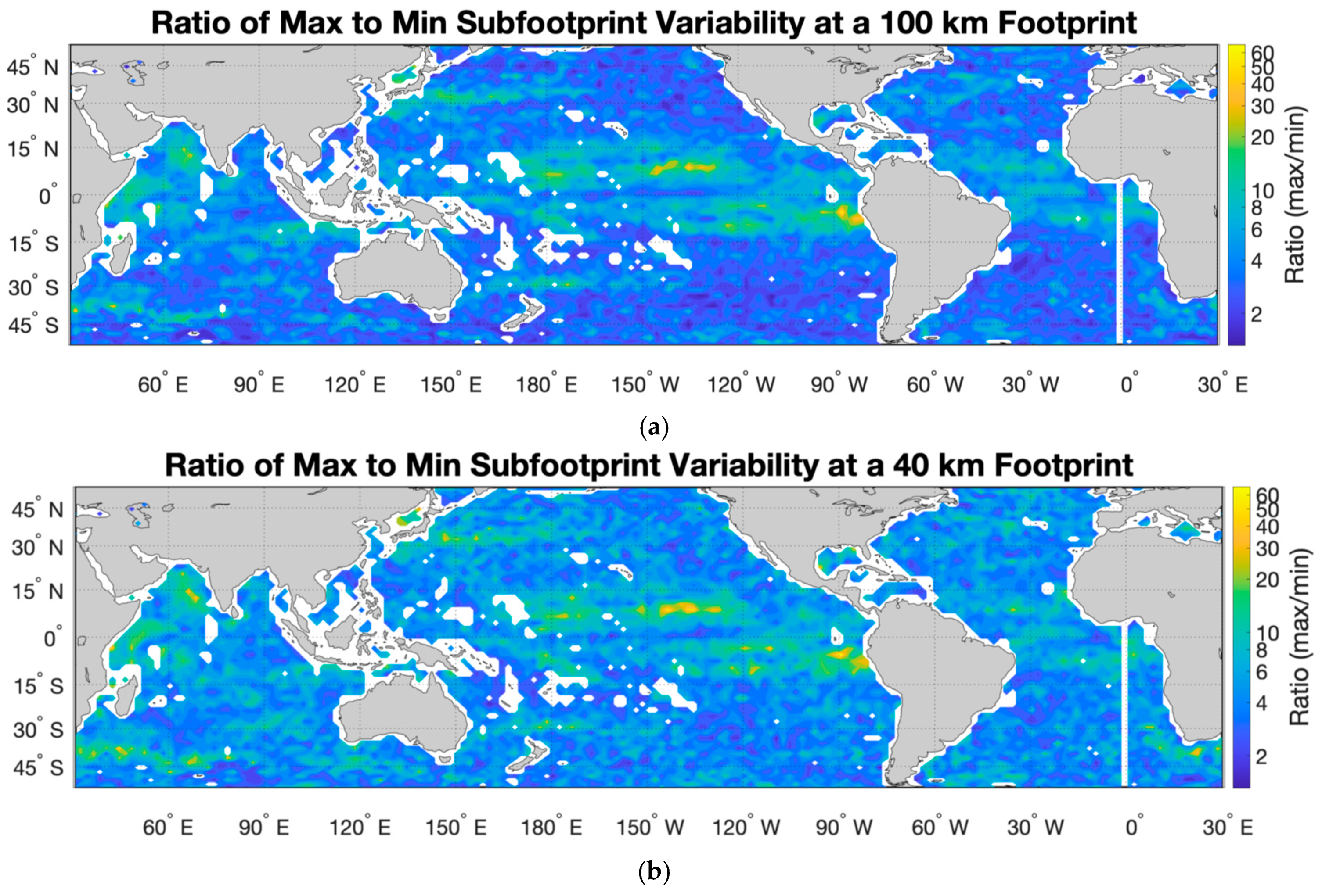
A similar picture is obtained by taking the ratio of the maximum to minimum monthly median SFV (Figure 8). This has a similar pattern to the March/September ratio, but it is not tied to a particular month. The places where the ratio is large in Figure 7, e.g., under the ITCZ in the Pacific, are also places where the ratio is large in Figure 8. We show this quantity for both the 100 and 40 km footprint size to emphasize the fact that the variability of SFV gets larger with decreasing footprint size. In the open ocean, the ratio takes on values of 3–5 for the 100 km footprint vs. 5–10 for the 40 km footprint.
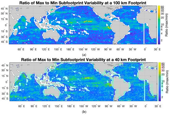
Figure 8.
Ratio of maximum monthly median SFV to minimum monthly median SFV for (a) 100 and (b) 40 km footprint size. Note the uneven logarithmic color scale on the right.
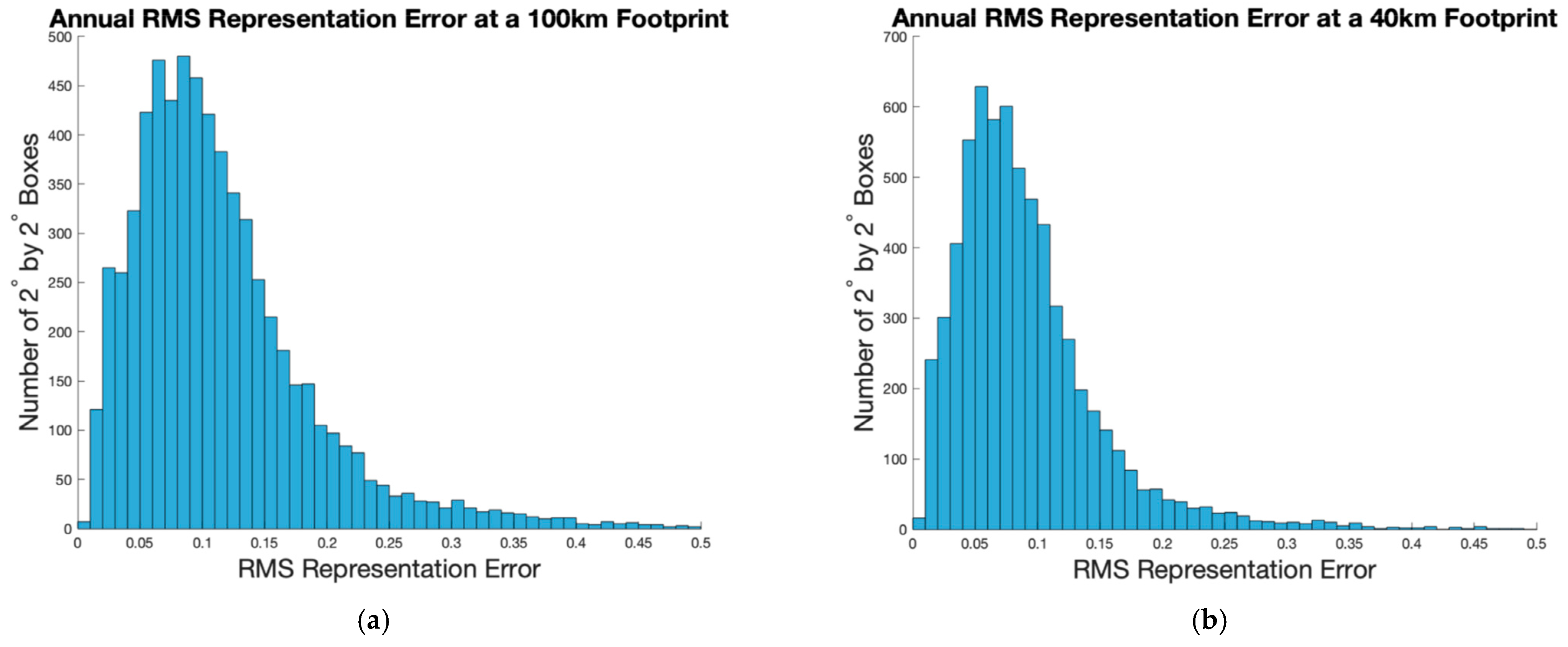
The distribution of RMS RE (Figure 9) looks similar to that of SFV (Figure 2), only the magnitudes are larger. For brevity, we do not include maps of RE here. They are very similar to those of Figure 2a,b. However, we do include them in Supplementary Materials Tables S4 and S5. The distribution at the 100 km (40 km) footprint, as seen in Figure 9a,b, can be compared to the SFV (Figure 2c,d). The RE for the 100 km (40 km) footprint has a mode at around 0.1 (0.06). The fact that the RE is larger than the SFV was also observed by Reference [20] for the tropics. It likely has to do with the characteristically negatively skewed distribution of SSS [35]. The magnitudes given by Reference [20], computed from tropical mooring data, are similar to the ones found here.

Figure 9.
As in Figure 2c,d, but for RMS RE instead of SFV. (a,b) Display the same RMS RE values as histograms, which count the number of 2° × 2° boxes with the given RMS RE for the full year. The total number of boxes in both figures is 10,440. Note different y-axis limits in the two panels.
4. Discussion
We have computed SFV using a global high-resolution model, and displayed maps of median SFV at 100 and 40 km footprint size (Figure 2a,b), the approximate sizes for the Aquarius and SMAP satellites. We have taken advantage of the high resolution of the version of the MITgcm simulation that we used, which has been shown to simulate mesoscale motions better than coarser versions [24]. The results we have found are similar in pattern and magnitude to those of Reference [16] as described in the introduction. Compare our Figure 2a with their Figure 2a. Our results are also similar in magnitude to those of Reference [17]—compare our Figure 2a with their Figure 9a. They used thermosalinograph data, not a model, and at a coarser resolution (3° × 3°), but found large variability in the same places we did. At a smaller scale, Reference [17] looked at variability at scales of 20 km or less from thermosalinograph data (see their Figure 4a). Their map compares well in detail with ours at 40 km or smaller scale (Figure 2b). The difference between our map and theirs is that their estimate includes variability at scales of 8 down to 2.5 km, whereas ours do not due to the effective resolution of the model. The fact that the details of our map match well with theirs gives confidence that there is not a lot of salinity variance at scales of 8 km or less that the model may be missing.
We have gone beyond those previous studies and examined the dependence of SFV on footprint size and season. This dependence has been hinted at by References [10,19] for two specific locations in the Tropical Pacific and Subtropical North Atlantic. Reference [20] also found strong seasonal variability in SFV (using a proxy measurement) for the global tropics, though they did not look at variation by footprint size.
SFV varies over the course of the year almost everywhere. Most of the ocean has largest SFV in the fall season (Figure 6 and Figure 7). The smallest effect is in the northern hemisphere south of 30° N (Figure 6). This latitude range is the location of bands of alternating fall and spring maxima in SFV shown in Figure 7, likely due to the seasonal migration of the North Equatorial Countercurrent front in the Tropical Atlantic and Pacific. These bands extend across the equator into the southern hemisphere and are prominent at both the 40 and 100 km scales (Figure 8). Outside of these tropical bands, in the open subtropical and subpolar ocean, SFV is more seasonally dependent at the 40 km size than at 100 km.
The obvious question is whether the seasonality of SFV is due to contrasting rainfall, seasonality in the ocean’s internal submesoscale variability, seasonal migration of large-scale fronts, such as the Kuroshio extension, or some other cause. There have been a number of studies of the seasonality of submesoscale variability in the ocean, as it relates to such quantities as eddy kinetic energy and vorticity [25,36,37,38]. These have generally found that there is a maximum of variability at the submesoscale in winter and spring, different from what we have shown here. For example, in an area of the Kuroshio extension, Reference [25] found, using the same model we did, that the strength of submesoscale turbulence is much larger in April than in October; this is almost completely opposite to our results. This suggests that the size of the SSS SFV is tied to the strength of the surface forcing more than the ocean submesoscale, at least at this location. The seasonality of SFV is elevated in some areas with large-scale fronts, such as the Kuroshio extension, Antarctic Circumpolar Current front southeast of Africa and the North Equatorial Countercurrent (NECC) front in the Tropical North Pacific (Figure 8). However, the same elevation is missing in other frontal regions, such as the Gulf Stream/North Atlantic Current and the Brazil–Malvinas Confluence. The seasonal motion of the NECC front is well known [33]. Seasonality in the position or strength of the Kuroshio extension front has not been reported (to the authors’ knowledge), so the elevated SFV seasonality there may be due to surface forcing. Keeping in mind that the results presented here are based on only one year of model output, a more definitive understanding of the seasonality of SFV awaits future study.
As just stated, one of the limitations of this study is the short (1 year) duration of the model record, which renders the study’s conclusions regarding seasonality tentative. It is not computationally practical to run a model at this high resolution for much longer than 1 year at present. Further verification of the results we have presented could be obtained by using a lower-resolution model, such as that used by Reference [16]. There has also been an effort to look at seasonality of SFV by using mooring data [20] and a proxy indicator. Understanding how SFV and RE vary seasonally is important for incorporation into satellite error budgets, and also as an intrinsically interesting and little explored area of study of upper ocean variability.
As expected, we show that SFV increases as a function of footprint size (Figure 4c,d,f and Figure 5). Reference [19] found the same for the SPURS-1 and SPURS-2 locations, using real in situ data. The curve we found for March for SPURS-2 (black curve in Figure 4c) matches well with the one in Reference [19] (their Figure 3b, dashed curve), whereas the one we found for September (black curve in Figure 4d) has a much stronger spatial dependence than theirs (Figure 3b in Reference [19], thick solid curve). For SPURS-1, the comparison was similar. Compare the blue curves in our Figure 4c,d with the thick solid and dashed curves in Figure 4 in Reference [19]. Thus, for the low SFV season, our results match those of Reference [19] well, but for the high SFV season, we found a much stronger dependence on footprint size and larger value of SFV.
It appears that SFV depends more strongly on footprint size in the fall season than in the spring. Figure 4c,d shows examples of this, whereas Figure 5 shows it in a more general way, comparing the top and bottom rows. One simple explanation lies in the seasonality of rainfall. Rainfall varies throughout the year, and it is maximum in the fall over most of the ocean (Figure 10). Rainfall generates SSS variance through the introduction of fresh patches at the surface [10,18,19,39,40,41]. Larger SSS variance means larger values of SFV, so it is not the amount of rainfall that matters in this case, but the seasonal distribution. It only takes a few small patches within a footprint to greatly increase the SFV. As the footprint size increases, the likelihood of the footprint incorporating patches of rain-induced low SSS increases, leading to increased SFV.
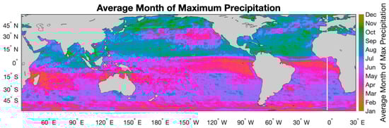
Figure 10.
Month of maximum precipitation from IMERG data. Monthly averaged values from June 2000 to May 2019 were used. For each year, the month with the maximum average precipitation value was recorded at each point in space, and then the mean of those 19 values was used as the average maximum month. Color scale is on the right.
Another interesting observation we have found here is that the seasonal range of SFV is larger for small footprint size than large (Figure 8). Perhaps this observation has to do with rainfall as well. The smaller the footprint, the more impact individual rain-induced patches have on SFV; thus, rainfall may impact the SSS variance more at a small scale than a large one.
We have not examined reasons why SFV might be elevated or depressed in particular locations in this paper (e.g., Figure 2a), but some statements can be made. As stated above, the distribution of SFV does not follow the distribution of total rainfall from Reference [30], among others. Thus, the total rainfall may not be a strong determinant of SFV. However, Reference [19] found good correlations between the maximum rain rate and SFV, especially at the SPURS-1 site. SFV may be determined by the maximum rain rate, i.e., how the rain falls, not the total rainfall at a particular location. This was also the conclusion of Reference [20] for the global tropics. Of course, SFV can also be elevated by proximity to fronts such as the Gulf Stream or coastal river plumes, such as those in the Bay of Bengal, as can be seen in Figure 2a,b.
The main purpose of this paper is to get estimates of SFV to include in error budgets for satellites. SFV itself is small and mostly insignificant relative to other sources of error [4,6,42]. At a 100 km (40 km) footprint size, typical annual median values of SFV are about 0.02–0.15 (0.02–0.07). These are the peaks of the distributions from Figure 2c,d. There are some much larger values, as we have discussed, especially at 100 km footprint.
As a further iteration on this, we have computed an estimate of the RMS RE, which may be a better indicator to use for understanding the sampling issue with satellite SSS measurement. Values of RE are larger than SFV, with typical values of 0.02–0.20 (0.01–0.15) at a 100 km (40 km) footprint and peaks at about 0.1 (0.06). The Aquarius mission was predicated on a measurement accuracy of 0.2 over a 150 km spatial and 1-month timescale [6]. The analysis we performed here is not a direct comparison to that number. It is a determination of snapshot error, or the error associated with a single L2 measurement due to inadequate representation of variability within the footprint. Kao et al. [5] computed the RMS snapshot error for real Argo and Aquarius data and found it to be 0.17. Our results indicate that RE is likely a large fraction of that value. Similarly, Reference [15] computed RMS values of the snapshot error for SMAP and found a value of 0.49 (see their Figure 3b). Thus, RE is a much smaller fraction of the snapshot error for SMAP than for Aquarius. As indicated by the numbers just given, real snapshot errors are larger for SMAP than for Aquarius, but this is partially offset by the much larger numbers of snapshots collected by SMAP, due to its trochoidal sampling pattern [1]. Future work in this area will involve using the simulated satellite L2 and related simulated Argo [23] datasets we have generated to create simulated L3 products. With these, we can test how much SFV and RE contribute to the observed errors in Aquarius and SMAP at monthly timescales.
The nature of SFV or RE has been discussed at length elsewhere [10,20]. What has been less discussed is how, once these quantities are determined, they are to be incorporated into the satellite error budget. They have not been previously incorporated into satellite error estimates, such as those of References [12,43]. They are, in essence, a negative error in that they do not indicate measurement inaccuracy, and thus the satellites may be more accurate than previously understood. Exactly how SFV and RE should be used in quantifying SSS satellite accuracy is a subject for further study.
5. Conclusions
We computed the SFV of SSS for a 100 and 40 km footprint size from a global (non-Arctic) high-resolution model. SFV is the weighted standard deviation of SSS within the satellite footprint (Figure 1 and Equations (1) and (2)). We presented maps of the median value of this quantity for a full year (Figure 2a,b) and for a couple of selected months for 100 km (Figure 3). Typical median values are 0.02–0.15 (0.02–0.07) for a 100 (40) km footprint (Figure 2c,d). The mode of the distribution is 0.06 (0.04) for a 100 (40) km footprint. We also examined RE and found typical values of 0.02–0.20 (0.01–0.15) for a 100 (40) km footprint (Figure 9). RE is the deviation between the footprint-weighted mean and a randomly chosen model value within the footprint. The mode of the RE distribution is 0.1 (0.06). We computed the distribution of SFV as a function of footprint size and found that it increases as expected (Figure 5). The variation relative to footprint size is a function of season and location (e.g., see Figure 4).
We looked at the seasonal variability of SFV (Figure 8) and RE and found that it is usually maximum in the fall season (Figure 3 and Figure 5, Figure 6, Figure 7), and tends to be larger in the northern hemisphere than the southern. The seasonality is consistent with the pattern of maximum rainfall (Figure 10), though, as discussed above, the connection between rainfall and SFV is still to be worked out.
Future work will involve understanding the connection between rainfall and SFV, extending the present analysis to quantify RE at L3 and working out the spatial scales of SFV and RE.
Supplementary Materials
The following are available online at https://www.mdpi.com/article/10.3390/rs13214410/s1. Tables S1–S5.
Author Contributions
Conceptualization, F.M.B. and S.F.; methodology, F.M.B. and H.Z.; software, S.B., A.H. and K.U.; validation, F.M.B., A.H. and S.B.; resources, S.F. and F.M.B.; data curation, H.Z.; writing—original draft preparation, F.M.B.; writing—review and editing, F.M.B. and S.F.; visualization, S.B. and K.U.; supervision, S.F.; project administration, S.F. and F.M.B.; funding acquisition, S.F. and F.M.B. All authors have read and agreed to the published version of the manuscript.
Funding
Part of the research described in this paper was carried out at the Jet Propulsion Laboratory, California Institute of Technology, under a contract with NASA. This research was supported by NASA under grants 19-OSST19-0007 and 80NSSC18K1322.
Data Availability Statement
Data used in this study can be found at the following locations: MITgcm SSS: https://catalog.pangeo.io/browse/master/ocean/LLC4320/LLC4320_SSS/ (accessed on 1 June 2020); IMERG rainfall: https://doi.org/10.5067/GPM/IMERG/3B-MONTH/06 (accessed on 1 October 2020).
Acknowledgments
Color scales for many figures in this paper were taken from the “cmocean” package [44]. We appreciate the careful reading and suggestions of three anonymous reviewers.
Conflicts of Interest
The authors declare no conflict of interest.
References
- Reul, N.; Grodsky, S.; Arias, M.; Boutin, J.; Catany, R.; Chapron, B.; D’Amico, F.; Dinnat, E.; Donlon, C.; Fore, A.; et al. Sea surface salinity estimates from spaceborne L-band radiometers: An overview of the first decade of observation (2010–2019). Remote Sens. Environ. 2020, 242, 111769. [Google Scholar] [CrossRef]
- Reul, N.; Fournier, S.; Boutin, J.; Hernandez, O.; Maes, C.; Chapron, B.; Alory, G.; Quilfen, Y.; Tenerelli, J.; Morisset, S.; et al. Sea Surface Salinity Observations from Space with the SMOS Satellite: A New Means to Monitor the Marine Branch of the Water Cycle. Surv. Geophys. 2014, 35, 681–722. [Google Scholar] [CrossRef] [Green Version]
- Vinogradova, N.; Lee, T.; Boutin, J.; Drushka, K.; Fournier, S.; Sabia, R.; Stammer, D.; Bayler, E.; Reul, N.; Gordon, A.; et al. Satellite Salinity Observing System: Recent Discoveries and the Way Forward. Front. Mar. Sci. 2019, 6, 243. [Google Scholar] [CrossRef]
- Meissner, T.; Wentz, F.J.; Le Vine, D.M. The Salinity Retrieval Algorithms for the NASA Aquarius Version 5 and SMAP Version 3 Releases. Remote Sens. 2018, 10, 1121. [Google Scholar] [CrossRef] [Green Version]
- Kao, H.-Y.; Lagerloef, G.S.E.; Lee, T.; Melnichenko, O.; Meissner, T.; Hacker, P. Assessment of Aquarius Sea Surface Salinity. Remote Sens. 2018, 10, 1341. [Google Scholar] [CrossRef] [Green Version]
- Lagerloef, G.; Colomb, F.R.; Le Vine, D.; Wentz, F.; Yueh, S.; Ruf, C.; Lilly, J.; Gunn, J.; Chao, Y.; Decharon, A.; et al. The Aquarius/SAC-D Mission: Designed to Meet the Salinity Remote-Sensing Challenge. Oceanograph 2008, 21, 68–81. [Google Scholar] [CrossRef] [Green Version]
- Yueh, S.; West, R.; Wilson, W.; Li, F.; Njoku, E.; Rahmat-Samii, Y. Error sources and feasibility for microwave remote sensing of ocean surface salinity. IEEE Trans. Geosci. Remote Sens. 2001, 39, 1049–1060. [Google Scholar] [CrossRef] [Green Version]
- Meissner, T.; Wentz, F.; Manaster, A.; Lindsley, R. NASA/RSS SMAP Salinity: Version 4.0 Validated Release, Release Notes, Algorithm Theoretical Basis Document (ATBD). RSS Technical Report 082219. 22 August 2019. Available online: https://data.remss.com/smap/SSS/Release_V4.0.pdf (accessed on 14 July 2021).
- D’Addezio, J.M.; Bingham, F.; Jacobs, G.A. Sea surface salinity subfootprint variability estimates from regional high-resolution model simulations. Remote Sens. Environ. 2019, 233, 111365. [Google Scholar] [CrossRef]
- Bingham, F.M. Subfootprint Variability of Sea Surface Salinity Observed during the SPURS-1 and SPURS-2 Field Campaigns. Remote Sens. 2019, 11, 2689. [Google Scholar] [CrossRef] [Green Version]
- Abe, H.; Ebuchi, N. Evaluation of sea-surface salinity observed by Aquarius. J. Geophys. Res. Ocean. 2014, 119, 8109–8121. [Google Scholar] [CrossRef]
- Tang, W.; Fore, A.; Yueh, S.; Lee, T.; Hayashi, A.; Sanchez-Franks, A.; Martinez, J.; King, B.; Baranowski, D. Validating SMAP SSS with in situ measurements. Remote Sens. Environ. 2017, 200, 326–340. [Google Scholar] [CrossRef] [Green Version]
- Kao, H.-Y.; Lagerloef, G.; Lee, T.; Melnichenko, O.; Hacker, P. Aquarius Salinity Validation Analysis, Data Version 5.0; Aquarius/SAC-D: Seattle, WA, USA, 2018; p. 45.
- Bao, S.; Wang, H.; Zhang, R.; Yan, H.; Chen, J. Comparison of Satellite-Derived Sea Surface Salinity Products from SMOS, Aquarius, and SMAP. J. Geophys. Res. Ocean. 2019, 124, 1932–1944. [Google Scholar] [CrossRef]
- Qin, S.; Wang, H.; Zhu, J.; Wan, L.; Zhang, Y.; Wang, H. Validation and correction of sea surface salinity retrieval from SMAP. Acta Oceanol. Sin. 2020, 39, 148–158. [Google Scholar] [CrossRef]
- Vinogradova, N.T.; Ponte, R.M. Small-Scale Variability in Sea Surface Salinity and Implications for Satellite-Derived Measurements. J. Atmos. Ocean. Technol. 2013, 30, 2689–2694. [Google Scholar] [CrossRef]
- Drushka, K.; Asher, W.E.; Sprintall, J.; Gille, S.T.; Hoang, C. Global Patterns of Submesoscale Surface Salinity Variability. J. Phys. Oceanogr. 2019, 49, 1669–1685. [Google Scholar] [CrossRef]
- Boutin, J.; Chao, Y.; Asher, W.E.; Delcroix, T.; Drucker, R.; Drushka, K.; Kolodziejczyk, N.; Lee, T.; Reul, N.; Reverdin, G.; et al. Satellite and In Situ Salinity: Understanding Near-Surface Stratification and Subfootprint Variability. Bull. Am. Meteorol. Soc. 2016, 97, 1391–1407. [Google Scholar] [CrossRef] [Green Version]
- Bingham, F.; Li, Z. Spatial Scales of Sea Surface Salinity Subfootprint Variability in the SPURS Regions. Remote Sens. 2020, 12, 3996. [Google Scholar] [CrossRef]
- Bingham, F.M.; Brodnitz, S. Sea surface salinity short-term variability in the tropics. Ocean Sci. 2021, 17, 1437–1447. [Google Scholar] [CrossRef]
- Bingham, F.M.; Li, P.; Li, Z.; Vu, Q.; Chao, Y. Data Management Support for the SPURS Atlantic Field Campaign. Oceanography 2015, 28, 46–55. [Google Scholar] [CrossRef] [Green Version]
- Li, Z.; California Institute of Technology; Bingham, F.; Li, P. Multiscale Simulation, Data Assimilation, and Forecasting in Support of the SPURS-2 Field Campaign. Oceanography 2019, 32, 134–141. [Google Scholar] [CrossRef]
- Bingham, F.; Fournier, S.; Brodnitz, S.; Ulfsax, K.; Zhang, H. Matchup Characteristics of Sea Surface Salinity Using a High-Resolution Ocean Model. Remote Sens. 2021, 13, 2995. [Google Scholar] [CrossRef]
- Su, Z.; Wang, J.; Klein, P.; Thompson, A.F.; Menemenlis, D. Ocean submesoscales as a key component of the global heat budget. Nat. Commun. 2018, 9, 1–8. [Google Scholar] [CrossRef] [Green Version]
- Rocha, C.B.; Gille, S.T.; Chereskin, T.K.; Menemenlis, D. Seasonality of submesoscale dynamics in the Kuroshio Extension. Geophys. Res. Lett. 2016, 43, 11–304. [Google Scholar] [CrossRef]
- Su, Z.; Torres, H.; Klein, P.; Thompson, A.F.; Siegelman, L.; Wang, J.; Menemenlis, D.; Hill, C. High-frequency Submesoscale Motions Enhance the Upward Vertical Heat Transport in the Global Ocean. J. Geophys. Res. Oceans 2020, 125, 016544. [Google Scholar] [CrossRef]
- Adcroft, A.; Campin, J.-M.; Doddridge, E.; Dutkiewicz, S.; Evangelinos, C.; Ferreira, D.; Follows, M.; Forget, G.; Fox-Kemper, B.; Heimbach, P.; et al. Welcome to MITgcm’s User Manual. Available online: https://mitgcm.readthedocs.io/en/latest/ (accessed on 9 August 2021).
- Vazquez-Cuervo, J.; Gentemann, C.; Tang, W.; Carroll, D.; Zhang, H.; Menemenlis, D.; Gomez-Valdes, J.; Bouali, M.; Steele, M. Using Saildrones to Validate Arctic Sea-Surface Salinity from the SMAP Satellite and from Ocean Models. Remote Sens. 2021, 13, 831. [Google Scholar] [CrossRef]
- Menemenlis, D.; Campin, J.-M.; Heimbach, P.; Hill, C.; Lee, T.; Nguyen, A.; Schodlok, M.; Zhang, H. ECCO2: High Resolution Global Ocean and Sea Ice Data Synthesis. Mercator Ocean Q. Newsl. 2008, 31, 13–21. [Google Scholar]
- Schanze, J.J.; Schmitt, R.W.; Yu, L.L. The global oceanic freshwater cycle: A state-of-the-art quantification. J. Mar. Res. 2010, 68, 569–595. [Google Scholar] [CrossRef]
- Lindstrom, E.; Bryan, F.; Schmitt, R. SPURS: Salinity Processes in the Upper-ocean Regional Study—The North Atlantic Experiment. Oceanography 2015, 28, 14–19. [Google Scholar] [CrossRef] [Green Version]
- Lindstrom, E.; Edson, J.; Schanze, J.; Shcherbina, A. SPURS-2: Salinity Processes in the Upper-Ocean Regional Study 2—The Eastern Equatorial Pacific Experiment. Oceanography 2019, 32, 15–19. [Google Scholar] [CrossRef]
- Melnichenko, O.; University of Hawaii; Hacker, P.; Bingham, F.; Lee, T. Patterns of SSS Variability in the Eastern Tropical Pacific: Intraseasonal to Interannual Timescales from Seven Years of NASA Satellite Data. Oceanography 2019, 32, 20–29. [Google Scholar] [CrossRef]
- Kessler, W.S. The circulation of the eastern tropical Pacific: A review. Prog. Oceanogr. 2006, 69, 181–217. [Google Scholar] [CrossRef]
- Bingham, F.M.; Howden, S.D.; Koblinsky, C.J. Sea surface salinity measurements in the historical database. J. Geophys. Res. 2002, 107, 8019. [Google Scholar] [CrossRef]
- Sasaki, H.; Klein, P.; Qiu, B.; Sasai, Y. Impact of oceanic-scale interactions on the seasonal modulation of ocean dynamics by the atmosphere. Nat. Commun. 2014, 5, 1–8. [Google Scholar] [CrossRef] [Green Version]
- Buckingham, C.E.; Garabato, A.C.N.; Thompson, A.F.; Brannigan, L.; Lazar, A.; Marshall, D.P.; Nurser, A.J.G.; Damerell, G.; Heywood, K.J.; Belcher, S.E. Seasonality of submesoscale flows in the ocean surface boundary layer. Geophys. Res. Lett. 2016, 43, 2118–2126. [Google Scholar] [CrossRef] [Green Version]
- Callies, J.; Ferrari, R.; Klymak, J.; Gula, J. Seasonality in submesoscale turbulence. Nat. Commun. 2015, 6, 1–8. [Google Scholar] [CrossRef] [Green Version]
- Drushka, K.; University of Washington; Asher, W.; Jessup, A.; Thompson, E.; Iyer, S.; Clark, D. Capturing Fresh Layers with the Surface Salinity Profiler. Oceanography 2019, 32, 76–85. [Google Scholar] [CrossRef]
- Drushka, K.; Asher, W.E.; Ward, B.; Walesby, K. Understanding the formation and evolution of rain-formed fresh lenses at the ocean surface. J. Geophys. Res. Ocean 2016, 121, 2673–2689. [Google Scholar] [CrossRef] [Green Version]
- Thompson, E.; University of Washington; Asher, W.; Jessup, A.; Drushka, K. High-Resolution Rain Maps from an X-band Marine Radar and Their Use in Understanding Ocean Freshening. Oceanography 2019, 32, 58–65. [Google Scholar] [CrossRef]
- Olmedo, E.; González-Haro, C.; Hoareau, N.; Umbert, M.; González-Gambau, V.; Martínez, J.; Gabarró, C.; Turiel, A. Nine years of SMOS sea surface salinity global maps at the Barcelona Expert Center. Earth Syst. Sci. Data 2021, 13, 857–888. [Google Scholar] [CrossRef]
- Tang, W.; Yueh, S.H.; Fore, A.G.; Hayashi, A.; Lee, T.; Lagerloef, G. Uncertainty of Aquarius sea surface salinity retrieved under rainy conditions and its implication on the water cycle study. J. Geophys. Res. Oceans 2014, 119, 4821–4839. [Google Scholar] [CrossRef] [Green Version]
- Thyng, K.; Greene, C.; Hetland, R.; Zimmerle, H.; DiMarco, S. True Colors of Oceanography: Guidelines for Effective and Accurate Colormap Selection. Oceanography 2016, 29, 9–13. [Google Scholar] [CrossRef] [Green Version]

Publisher’s Note: MDPI stays neutral with regard to jurisdictional claims in published maps and institutional affiliations. |
© 2021 by the authors. Licensee MDPI, Basel, Switzerland. This article is an open access article distributed under the terms and conditions of the Creative Commons Attribution (CC BY) license (https://creativecommons.org/licenses/by/4.0/).