Article

Deep/Transfer Learning with Feature Space Ensemble Networks (FeatSpaceEnsNets) and Average Ensemble Networks (AvgEnsNets) for Change Detection Using DInSAR Sentinel-1 and Optical Sentinel-2 Satellite Data Fusion

by
Zainoolabadien Karim
1,*,†,‡ and
Terence L. van Zyl
2,†,‡
1
School of Computer Science and Applied Mathematics, University of the Witwatersrand, Johannesburg 2000, South Africa
2
Institute for Intelligent Systems, University of Johannesburg, Johannesburg 2000, South Africa
*
Author to whom correspondence should be addressed.
These authors contributed equally to this work.
This paper is an extended version of our paper published in the 2020 International SAUPEC/RobMech/PRASA Conference, Cape Town, South Africa, 29–31 January 2020.
Remote Sens. 2021, 13(21), 4394; https://doi.org/10.3390/rs13214394
Submission received: 8 September 2021 / Revised: 22 October 2021 / Accepted: 24 October 2021 / Published: 31 October 2021

Abstract

:
Differential interferometric synthetic aperture radar (DInSAR), coherence, phase, and displacement are derived from processing SAR images to monitor geological phenomena and urban change. Previously, Sentinel-1 SAR data combined with Sentinel-2 optical imagery has improved classification accuracy in various domains. However, the fusing of Sentinel-1 DInSAR processed imagery with Sentinel-2 optical imagery has not been thoroughly investigated. Thus, we explored this fusion in urban change detection by creating a verified balanced binary classification dataset comprising 1440 blobs. Machine learning models using feature descriptors and non-deep learning classifiers, including a two-layer convolutional neural network (ConvNet2), were used as baselines. Transfer learning by feature extraction (TLFE) using various pre-trained models, deep learning from random initialization, and transfer learning by fine-tuning (TLFT) were all evaluated. We introduce a feature space ensemble family (FeatSpaceEnsNet), an average ensemble family (AvgEnsNet), and a hybrid ensemble family (HybridEnsNet) of TLFE neural networks. The FeatSpaceEnsNets combine TLFE features directly in the feature space using logistic regression. AvgEnsNets combine TLFEs at the decision level by aggregation. HybridEnsNets are a combination of FeatSpaceEnsNets and AvgEnsNets. Several FeatSpaceEnsNets, AvgEnsNets, and HybridEnsNets, comprising a heterogeneous mixture of different depth and architecture models, are defined and evaluated. We show that, in general, TLFE outperforms both TLFT and classic deep learning for the small dataset used and that larger ensembles of TLFE models do not always improve accuracy. The best performing ensemble is an AvgEnsNet (84.862%) comprised of a ResNet50, ResNeXt50, and EfficientNet B4. This was matched by a similarly composed FeatSpaceEnsNet with an F1 score of 0.001 and variance of 0.266 less. The best performing HybridEnsNet had an accuracy of 84.775%. All of the ensembles evaluated outperform the best performing single model, ResNet50 with TLFE (83.751%), except for AvgEnsNet 3, AvgEnsNet 6, and FeatSpaceEnsNet 5. Five of the seven similarly composed FeatSpaceEnsNets outperform the corresponding AvgEnsNet.

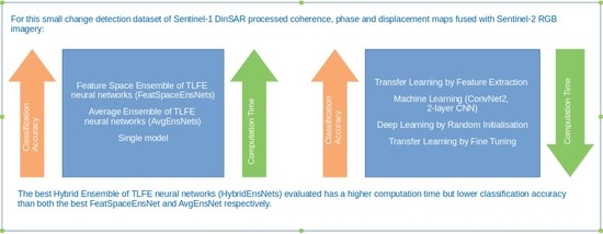
Graphical Abstract

1. Introduction

The European Space Agency’s Sentinel satellite missions and free remote sensing satellite imagery data have supported an increase in wide-area monitoring and evaluation. The Sentinel-1 constellation (Sentinel-1A and Sentinel-1B) provides C-band Synthetic Aperture Radar (SAR) data, is less affected by weather conditions, and can operate day and night. SAR data allow for the generation of interferometric synthetic aperture radar (InSAR) and the more advanced differential interferometric synthetic aperture radar (DInSAR) products that have been used for monitoring infrastructure as well as other geological phenomena [1,2,3,4,5].
For instance, Khalil and Haque [6] used a combination of Sentinel-1 SAR backscattered intensity, backscatter difference, and InSAR coherence for land cover classification, using a maximum likelihood classifier, and concluded that it was effective [6]. They note that the temporal gap between images was detrimentally long. The resulting decrease in coherence reduced discrimination between low and dense vegetated areas. Others, such as Corradino et al. [7], mapped lava flows at the Mount Etna volcano using a k-medoids unsupervised pixel-level classifier applied to Sentinel-2 multispectral imagery. A Bayesian Neural Network is also applied since the unsupervised classifier does not allow recent and older lava flow pixels to be differentiated. They indicate that if 0.02% of the lava flow field is known, the algorithm can detect the primary area of the lava flow, and a low-quality map of the flow can be obtained.
Sentinel-1 SAR data can be combined with Sentinel-2 optical imagery to improve results in numerous applications. For example, Van Tricht et al. [8] used a random forest to classify crops into several classes. They conclude that combining SAR backscatter data with the Sentinel-2 normalized difference vegetation index (NDVI) improves classification accuracy (82% with a kappa coefficient of 0.77) [8]. Gašparović et al. [9] fuse Sentinel-1 and Sentinel-2 data for flood mapping using a radial basis function (RBF) support vector machine (SVM) for object-based image analysis. They note that the method is fast compared to pixel-level techniques, and since it is an object/scene-based image classification, additional features of an object/scene are included with the optical signature. They compared the classification accuracy using varying sets of features. Using only the statistical first-order histogram and the geometric VH and VV polarized images result in an accuracy performance of 72.15% and 77.22%, respectively. Adding textural SAR images and optical features result in an accuracy increase to 87.34%. Furthermore, adding vegetation indices yields an accuracy of 89.87%. Finally, the optical bands’ statistical features are included and result in an accuracy of 94.94% [9].

1.1. Deep Learning

The advent of deep learning has significantly improved the accuracy of object recognition and image classification tasks [10,11]. Papadomanolaki et al. [12] applied it to optical images from Sentinel-2 to detect changes in urban areas. They used a convolutional neural network (CNN) for feature representation and a recurrent neural network (RNN) in the form of long short-term memory (LSTM) for temporal modeling. They found that the addition of fully convolutional LSTM layers to the U-net architecture improved accuracy and F1-score on the Onera Satellite Change Detection (OSCD) Sentinel-2 dataset [12]. Saha et al. [13] used an unsupervised deep learning-based method to detect a change in Sentinel-2 optical imagery using all 13 bands; they concluded that it is a more effective method of detecting change over using only the usual optical bands, with a disadvantage being the longer computation time required for training and classification [13].
Deep learning is also applied to Sentinel-1 and Sentinel-2 fused imagery. Ienco et al. [14] used a time series of Sentinel-1 SAR backscatter intensity data and Sentinel-2 optical data fed into two identical pipelines in the TWINNS network. They noted that the sensitivity to the noise, due to topography, in backscattering of the Sentinel-1 SAR intensity data resulted in a classifier that uses only the Sentinel-2 data outperforming one that used only the Sentinel-1 data. They did, however, find that fusing the datasets lead to better performance over both the Reunion Island and the Koumbia datasets from 73.89% and 81.94% when using only the Sentinel-1 data, respectively, and 84.26% and 81.99% when using only the Sentinel-2 data, respectively, to 89.88% and 87.50%, respectively, when fusing the datasets. This is since Sentinel-1 and Sentinel-2 data provide complimentary information [14]. A number of other experiments were also conducted applying a random forest classifier to just the combined Sentinel-1 and Sentinel-2 data fused at feature level, two random forest classifiers fused at decision level (late fusion), a random forest classifier applied to the entire TWINNS network and a convLSTM model. The best average accuracy obtained over the Reunion Island land cover classification task is 90.10% using the TWINNS network as a feature extractor with a random forest classifier, which improved performance compared to using just the TWINNS network (89.88%). However, no improvement was seen using the Koumbia land cover classification dataset using these other experiments as the best performing classifier is the TWINNS network (87.50%), whilst the second best performing classifier, which uses the TWINNS network as a feature extractor with a Random Forest classifier, only achieves 86.5% [14].
Gargiulo et al. [15] used multitemporal Sentinel-1 imagery combined with Sentinel-2 imagery over the Albufera Lagoon in Valencia to generate segmentation maps in areas where cloud cover affects the land cover mapping. A deep learning CNN, named W-net, is developed that results in an increase in performance at a lower computational cost compared to just using the Sentinel-2 imagery [15].
Sun et al. [16] used deep learning with InSAR imagery for detecting dynamic spatiotemporal patterns of displacement due to volcanic activity. They used it to efficiently de-noise multitemporal displacements acquired from the InSAR generated time series with a modified U-net CNN architecture. First, synthetic displacement maps are used to train a CNN. The pre-trained CNN is then used on real world data [16].

1.2. Transfer Learning

The above-mentioned increased accuracy from deep learning comes at an expense of requiring larger datasets and training times [10,11]. However, this limitation can to some extent be overcome using transfer learning [17]. Applying transfer learning from pre-trained models on large datasets benefits us by allowing for the increased accuracy of deep learning without incurring the full computational cost of training a deep neural network (DNN) from random initialization [1,4,18].
Transfer learning was previously applied to Sentinel-1 SAR and Sentinel-2 optical imagery. For instance, Pomente et al. [19] extract deep features from Sentinel-2 imagery acquired at different times using CNNs. A dissimilarity map with change probabilities at a pixel level was then developed by using the Euclidean distance between pixels. The areas where change occurred were indicated by bounding boxes and obtained by applying clustering with an optimizing connected component labeling algorithm. They concluded that the algorithm is effective [19].
Qiu et al. [20] used a ResNeXt DNN with multi-seasonal Sentinel-2 optical imagery to map human settlements [1,20]. GoogLeNet and ResNet50 were applied by Helber et al. [21] via transfer learning on optical images from Sentinel-2 for land use and land cover image classification. Performance accuracies of 98.18% and 98.57%, respectively, are realized with transfer learning with ResNet50 outperforming transfer learning with GoogLeNet. A labeled georeferenced Sentinel-2 based dataset containing 27,000 images was developed consisting of ten classes called EuroSAT [21]. Wang et al. [22] applied transfer learning to Sentinel-1 SAR images to automatically classify the wave mode images over the ocean into ten geophysical classes. They concluded that the algorithm is effective. They noted the occurrence of images that contained a mixture of a number of air-ocean processes and that were ambiguous [22]. Wang et al. [23] applied transfer learning with a Single Shot MultiBox Detector (SSD) to Sentinel-1 imagery to detect ships in the ocean with difficult surroundings, such as a mixture of islands and ocean. They found that the 512 × 512 pixel version outperformed the 300 × 300 pixel input version [23].
Anantrasirichai et al. [24] used transfer learning from the AlexNet CNN to detect volcanic ground motion in a large dataset of Sentinel-1 imagery containing more than 30,000 interferograms at 900 volcanoes. The system developed is able to detect rapid large scale deformations, but cannot detect deformations that are slow or of a small scale nature [24]. Anantrasirichai et al. [25] and Brengman et al. [26] both used transfer learning in other ground deformation applications [25,26]. Brengman et al. used a SarNet CNN with transfer learning from a synthetic dataset to a real dataset. SarNet achieved an accuracy of 85.22% on a real interferogram dataset [26].

1.3. Aim and Contribution

Ensembles have been shown to increase accuracy and stabilize the results for varying signal-to-noise ratios and deformation rates in previous work and in other domains [16,27]. Transfer learning was proven effective at bringing the increased accuracy of deep learning to smaller data sets at reduced computational cost. Having an understanding of how these techniques might be combined to improve change detection on a relatively small urban change detection dataset is of practical and theoretical importance. Unfortunately, limited (if any) research has been done to organize current approaches to ensemble leaning in a transfer learning paradigm [16]. Furthermore, little empirical evidence has been created to evaluate how these different methods might compare and how they stack up against non-deep learning approaches.
This article evaluates binary classification for urban change detection and extends upon previous work [1,4]. A novel dataset was developed comprising Sentinel-2 optical RGB images fused with the corresponding Sentinel-1 DInSAR coherence, phase, and displacement maps [3] for binary classification for urban change detection. A blob detection algorithm was used to detect change (either subsidence or uplift blobs) in the 2–14 July 2018, Terrain Corrected Displacement Map (Line of Sight) over Gauteng, South Africa [1,3,4].
There is a high false-positive rate; an automated machine learning binary classification approach improving upon previous work [1,4] was required. In this article, non-deep learning machine learning models using feature extraction algorithms, such as histogram of oriented gradients and local binary patterns were first evaluated as a baseline. A convolutional neural network with two layers (ConvNet2) was also evaluated [4]. A variety of DNN architectures as feature extractors were also analyzed. Transfer learning by fine-tuning (TLFT) and deep learning from random initialization (DLRI) were also evaluated using two models [1,4]. Ensembles of models used with transfer learning by feature extraction (TLFE) were also evaluated using a family of models, called feature space ensembles of TLFE neural networks (FeatSpaceEnsNets) and average ensembles of TLFE Neural Networks (AvgEnsNets). Seven FeatSpaceEnsNets, seven AvgEnsNets, and five hybrid ensembles of TLFE neural networks (HybridEnsNets) were defined and evaluated.

2. Materials and Methods

The methods used to generate the binary classification dataset as well as the classification algorithms used are discussed below.

2.1. Baseline Machine Learning Methods

To quantify the benefit of deep learning and transfer learning models over other approaches, some non-deep learning machine learning algorithms were evaluated as a baseline [28]. These include SVM, random forest, multi-layer perceptron, and a two-layer convolutional neural network (ConvNet2) discussed further below. The LBP and HOG feature vectors, as well as their combination, were fed into these non-deep learning classifiers. The Python [29] programming language was used with the Scikit-learn [30] and Scikit-image [31] machine learning libraries.

2.1.1. Linear SVM and Radial Basis Function (RBF) SVM

A linear support vector machine (Linear SVM) [32] classifier is a supervised machine learning algorithm that calculates a hyperplane that separates the different classes with the maximum separation between the hyperplane and the training data. In cases where the data are not linearly separable, a kernel can be used to map to a higher dimensional space, such as a radial basis function (RBF) kernel, i.e., RBF-SVM [32,33]. The regularization inverse, C, hyperparameter of the linear SVM classifier, is grid searched using the following values (0.001, 0.01, 0.1, 1.0, 10.0, 100.0) [4]. The regularization inverse, C, and the RBF kernel coefficient, gamma, hyperparameters of the RBF-SVM classifier, were grid searched both using the following values (0.001, 0.01, 0.1, 1.0, 10.0, 100.0) [4].

2.1.2. Random Forest (RF) and Multi-Layer Perceptron (MLP) Neural Network

A random forest (RF) [33,34,35] and multi-layer perceptron (MLP) neural network [32,33,36] classifiers were also evaluated on the feature vectors. Models with each feature descriptor alone and their combination were evaluated. A random forest is a supervised machine learning algorithm that uses an ensemble of decorrelated decision trees, which use a random set of features to split each node. In order to perform classification, the class that most trees voted for is yielded as the result [33,34,35]. The number of trees in the forest, n_estimators, hyperparameter of the random forest classifier was grid searched using the following values (50, 100, 150, 200, 250, 300).
A multi-layer perceptron (MLP) is an artificial neural network trained by the supervised machine learning method called backpropagation. It has an input layer, hidden layers with non-linear activation functions, and an output layer. It can be used to classify non-linear data [32,33,36]. The regularization, alpha, hyperparameter of the MLP classifier was grid searched using the following values (0.001, 0.01, 0.1, 1.0, 10.0, 100.0).

2.1.3. ConvNet2: Two Layer Convolutional Neural Network

A convolutional neural network (CNN) is an artificial neural network used for computer vision (or object recognition and classification) based on convolutional kernels applied to the input images to create feature maps instead of using feature descriptors [11]. A two-layer convolutional neural network (ConvNet2) was designed, which consists of two CNNs in parallel, one for the DInSAR processed Sentinel-1 images phase, coherence and displacement maps, and one for the Sentinel-2 optical images, as shown in Figure 1. The design of the CNN is similar to the ResNet convolutional blocks with two convolutional layers that have batch normalization and maximum pooling [11]. In the first 2D convolutional layer, there are 32 filters. In the second 2D convolutional layer, there are 64 filters. The convolutional layers use a 3 × 3 filter kernel and a ReLU activation function. A 2 × 2 filter kernel is used for maximum pooling. Thereafter, there is a Global Average Pooling layer [37]. This is followed by a dropout layer to avoid overfitting and to improve the model’s generalization [38]. The values, (0.2, 0.3, 0.4), are considered as the dropout hyperparameter to fine tune the model. Averaging of the Softmax output layers yields the ConvNet2’s output [4]. The two branches of the CNN were trained simultaneously in parallel. The Keras [39,40] library was used for implementing the ConvNet2 model and also for implementing the deep learning and transfer learning models.

2.2. Deep and Transfer Learning Methods

Deep learning models can have millions of parameters and require multiple GPUs and significant time to train using extensive datasets. Often, a sufficiently large dataset is not available for a DNN to achieve good performance. Transfer learning refers to transferring the knowledge gained from training a model with a sufficiently representative dataset to another task that may not have enough examples to train a DNN starting with random initialization. In this manner, knowledge is transferred from a well trained, much larger model, decreasing the computational cost required to train a DNN. This transfer is typically done using a pre-trained DNN and then replacing the final layer with one suited to the task at hand. A model with rich discriminative filters trained on the ImageNet dataset containing millions of images is often used as a pre-trained model in computer vision tasks [1,41]. From the three types of transfer learning possible, i.e., feature extraction, fine-tuning, and initializing with weights, the first two were implemented [1,4]. DLRI and transfer learning from models pre-trained on the ImageNet dataset were also implemented as part of this research.

2.2.1. Deep Learning and Transfer Learning using Fine-Tuning (TLFT)

Two pre-trained ResNet50 [42] models were combined, one for the stacked DInSAR processed Sentinel-1 phase, displacement, and coherence maps, and one for the RGB three-band image. This setup is used for classic deep learning (training from scratch, i.e., random initialization) and TLFT, since the built-in models cannot be used on six-band input imagery. The final Softmax predictive layer is removed from the built-in model. It is replaced with a global average pooling 2D layer, a dropout layer, and a customized Softmax layer suited to the number of classes, i.e., two classes for binary classification. These layers are added for each of the two built-in models. The final output of the model takes the average in the last layer. Early stopping is used for regularization to avoid overfitting the model to the training data. Dropout layers are also used to avoid overfitting [1]. The models are trained with the parallel branches of the networks trained simultaneously for a maximum of 50 epochs. The dropout hyperparameter was tuned using the following values, (0.2, 0.3, 0.4), and ten-fold cross-validation. Data augmentation with the following operations were applied to random images: zooming, shearing, height shifting, width shifting, horizontally flipping, or rotating [11].
To implement TLFT, first, all of the layers are frozen, and only the predictive layer is trained since the dataset is small [43]. Training is done with the parallel branches of the networks trained together for 50 epochs and uses early stopping, set to a value of four epochs of patience. After that, only the last convolutional layer is unfrozen in both of the parallel branches of the networks to be trained simultaneously with the last Softmax predictive layers in both branches of the network. Another round of training is done, which is also for 50 epochs with early stopping at the same patience interval as before. An optimizer (stochastic gradient descent) is used with a learning rate of 0.0001, which is slow. The optimizer also uses a momentum of 0.9. These parameters are used for training for both DLRI as well as TLFT [1,4].

2.2.2. Transfer Learning by Feature Extraction (TLFE)

In TLFE, the massive training cost associated with deep learning is eliminated. Numerous DNN architectures were used to implement TLFE. These models have weights pre-trained on the ImageNet dataset to generate feature maps and are used with the last predictive layer removed. A logistic regression classifier was trained on the feature maps that were generated using the pre-trained models. The regularization inverse hyperparameter (C) was tuned with values, (0.001, 0.0005, 0.0001). The logistic regression model was selected as it performed better than other linear models evaluated using the extracted features [1,4]. The difference between TLFE and TLFT is that no model training was required for the first method, i.e., the pre-trained model was directly applied to the new dataset to generate the feature maps.

2.3. Ensemble Methods

The ensemble of models can improve performance across a number of domains compared to single model performance if weak learners are aggregated by using voting [27,44,45,46]. Thus, ensembles of models were also evaluated with transfer learning using features extracted to generate feature maps. We then used Logistic Regression on the feature maps for classification. The average performance accuracy on a hold-out unseen test dataset obtained with ten-fold cross-validation was also measured [1,4]. Three types of ensembles were used: feature space ensemble of TLFE neural networks, average ensemble of TLFE neural networks, and hybrid ensemble of TLFE neural networks.

2.3.1. Feature Space Ensemble Networks (FeatSpaceEnsNets)

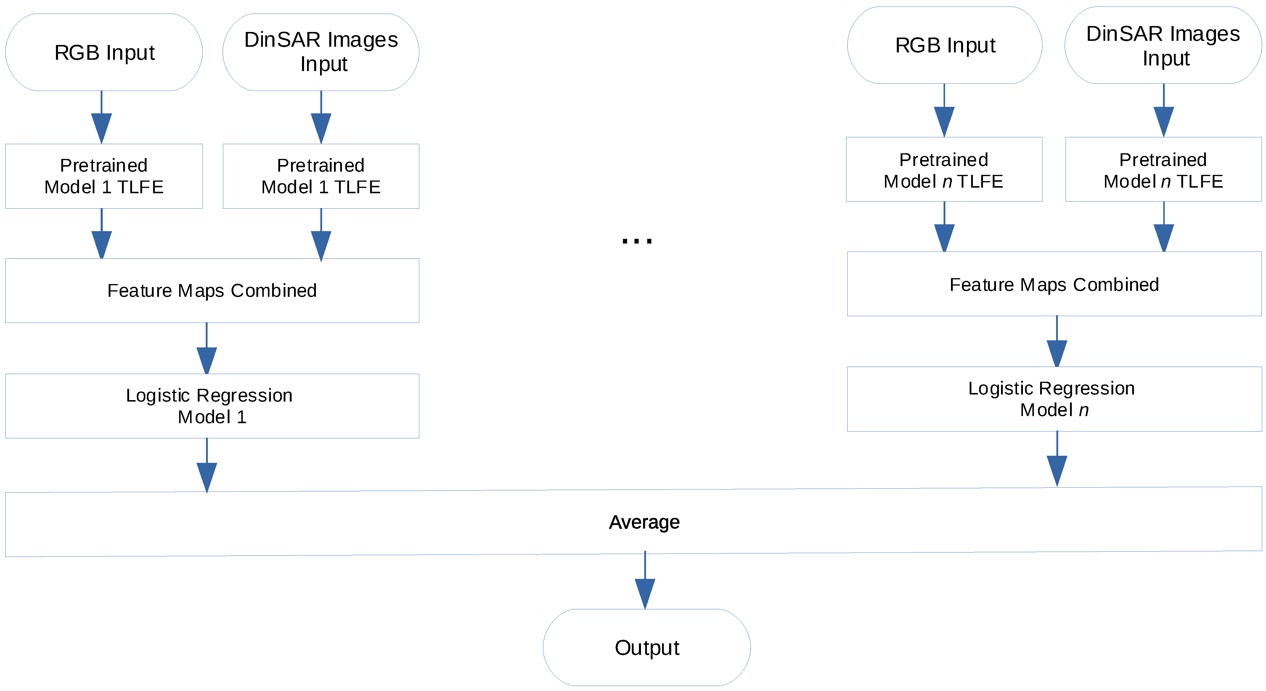
A FeatSpaceEnsNet is an ensemble of TLFE models ’ensembled’ in the feature space with one logistic regression classifier trained on the combined feature maps. Several different FeatSpaceEnsNets were evaluated using a mixture of DNNs to generate feature maps with only one logistic regression classifier applied to the combined feature maps. The general form of the architecture of the FeatSpaceEnsNet family of networks is shown in Figure 2 for pre-trained models 1 . . . n . The family of specific FeatSpaceEnsNets that have been implemented is shown in Table 1.

2.3.2. Average Ensemble Networks (AvgEnsNets)

An AvgEnsNet is an ensemble of TLFE models ’ensembled’ in the output space (decision level). Each model has its logistic regression classifier trained on only its feature maps. Then the outputs of the models in the ensemble are averaged to arrive at the final output of the AvgEnsNet. Several different AvgEnsNets were evaluated using a heterogeneous mixture of DNNs. The general form of the architecture of the AvgEnsNet family of DNNs is shown in Figure 3 for pre-trained models 1 . . . n . The family of specific AvgEnsNets that have been implemented is shown in Table 1.

2.3.3. Hybrid Ensemble Networks (HybridEnsNets)

A hybrid ensemble family of TLFE neural networks (HybridEnsNet) is also defined and evaluated as listed in Table 1. The HybridEnsNets include one FeatSpaceEnsNet model (FeatSpaceEnsNet 3, which is fused at the feature level) fused with an AvgEnsNet and single models (except HybridEnsNet 1) at the decision level. Thus, the HybridEnsNets contain models with a mixture of feature level and decision level fusion and fuses these models at the decision level.

2.4. Analysis of Methods

SVM performs well when data sets are small and dimensionality is high. SVM-RBF, RF, MLP, and deep learning methods function well with non-linearity, whilst the linear methods, SVM, make strong assumptions, which may not hold [32,33]. The deep learning methods generally require larger amounts of data to train [10,11].
The advent of deep residual networks (ResNet) [42] has allowed significantly deeper neural networks to be trained as they overcome the vanishing gradient problem by designing the layers, such that they learn residual functions of the layer inputs as opposed to learning unreferenced functions. This lead to improvements in image recognition accuracy. The ResNet50 has 50 layers, ResNet101 has 101 layers, and so on [1,4,42]. ResNet Version 2 (ResNetV2) [47] improved upon ResNet and is based upon a new residual unit that makes training simpler and improves generalization by using identity mappings as the skip connections and after-addition activation to improve accuracy [1,4,47].
An Inception [48] architecture uses multi-scale processing and its design keeps computational cost constant while expanding the depth and width of a DNN [48]. When residual connections are added to an Inception architecture, the resultant DNN is an Inception-ResNet architecture [49]. The residual connections drastically reduce the DNN training time [1,4,49].
The ResNeXt [50] architecture expands a DNN in a different dimension, which is the cardinality, i.e., the total transformations. It introduced the design of repeating a basic unit that is aggregating a group of transformations with similar architecture which is called “network in neuron” [1,4,50].
Tan et al. [51] noticed an increase in accuracy when scaling up the network depth, width and resolution parameters. The notion of a compound coefficient which uniformly scales each of these parameters was introduced. The EfficientNet [51] family of DNNs were designed using neural architecture search to yield a baseline network which was scaled up. EfficientNets are said to require less training time since they have less parameters compared to other comparable DNN architectures [1,4,51]. The more layers in a DNN, the more parameters it will have, and the more data it will require to be adequately trained. Thus, deeper neural networks perform better when there are more data available, than they do for smaller datasets [4].

2.5. Data

The European Space Agency’s Copernicus Open Access Data Hub [52] provides free imagery from the Sentinel satellite missions. In this research, Sentinel-1B SAR data and Sentinel-2 optical imagery were used. The Sentinel-1 satellites have a revisit frequency of six days over Europe and 12 days over Africa and can achieve spatial resolutions of up to 5 × 20 m [2]. Sentinel-2 provides optical RGB imagery data as well as multispectral data. Sentinel-2 can achieve spatial resolution of 10 m in the optical RGB bands [53]. Differential interferometric synthetic aperture radar (DInSAR) processing [54,55,56] of the interferometric wide swath mode SAR data were done using the Sentinel Application Platform (SNAP) Sentinel-1 toolbox [57] to produce a differential interferogram from single look complex (SLC) vertical–vertical polarized images over Gauteng, South Africa. Bursts 3 to 7 in IW swath 1 were used. To unwrap the differential interferogram, the statistical-cost network-flow algorithm for phase unwrapping (SNAPHU) software was used [58]. A terrain-corrected displacement map was generated. To process the optical Sentinel-2 images from Level 1C (top of atmosphere) images to atmospherically corrected Level 2A (bottom of atmosphere) images at a resolution of 10 m, the Sen2Cor software tool was employed [59].
For change (either subsidence or uplift blobs) to be detected in the 2–14 July 2018, Terrain Corrected Displacement Map (Line of Sight), the Laplacian of Gaussian [60] blob detection algorithm was used. There was a high false-positive rate due to the drop in coherence over vegetated areas. To overcome this issue, we used the blob detection algorithm as a candidate selection algorithm and we used a binary classification machine learning model to fine tune the classification of the candidates. For each blob phase, coherence and displacement maps were subsetted using the Geospatial Data Abstraction Library (GDAL) [61] and re-projected to the Sentinel-2 Coordinate Reference System for combination with the corresponding Sentinel-2 optical images obtained on 1 July 2018 and 16 July 2018. Effectively, each blob had 2 × 3 bands [1]. The resolution of the Sentinel-1 images was 28 × 34 m since 8 × 2 multi-looking (avg. pooling) was done to decrease the noise in the interferogram. The images were resized to 224 × 224 for all the models except for the InceptionResNetV2 [49], which used 299 × 299 . After processing, qualitative visual verification of the blobs was done using optical RGB Sentinel-2 images. At least 574 blobs required further verification using images from Google Earth [62] since the Sentinel-2 images alone were not sufficient to classify the blob (as false/true-positive) for manual data labeling purposes [1,4].

2.6. Data Preprocessing

The DInSAR processed images (phase, displacement, and coherence) were scaled to the RGB range from 0 to 255 for all of the models, excluding the non-deep machine learning models, as they used feature descriptors. Mean image subtraction preprocessing was used for the ResNet50 model. For the best performance to be obtained from transfer learning the same input image sizes and preprocessing needed to be performed, as what was performed when the model was trained on the original dataset [1,47]. Scaling the features to unit variance and zero mean preprocessing was done for the logistic regression models used when doing TLFE. The same scaling was also used for the support vector machines, random forest, and multi-layer perceptron models used in the non-deep machine learning models. This scaling helps to avoid skewing the model and caters for any features that may have a larger scale or variance than the rest of the features [4].

LBP and HOG Feature Descriptors

For feature extraction, the histogram of oriented gradients (HOG) [63,64] as well as the local binary pattern (LBP) [63] feature descriptors were used to generate feature vectors. The HOG descriptor aims to capture coarse spatial structure and was used originally for human pedestrian detection [64]. First, the image was normalized, then the image gradient was computed. Thereafter, the image was divided into cells and a local 1D histogram of gradients (edge orientations) for all of the pixels, which the cell contained, was computed. Then normalization in the HOG space across the blocks was performed, followed by flattening into a feature vector [63,64,65].
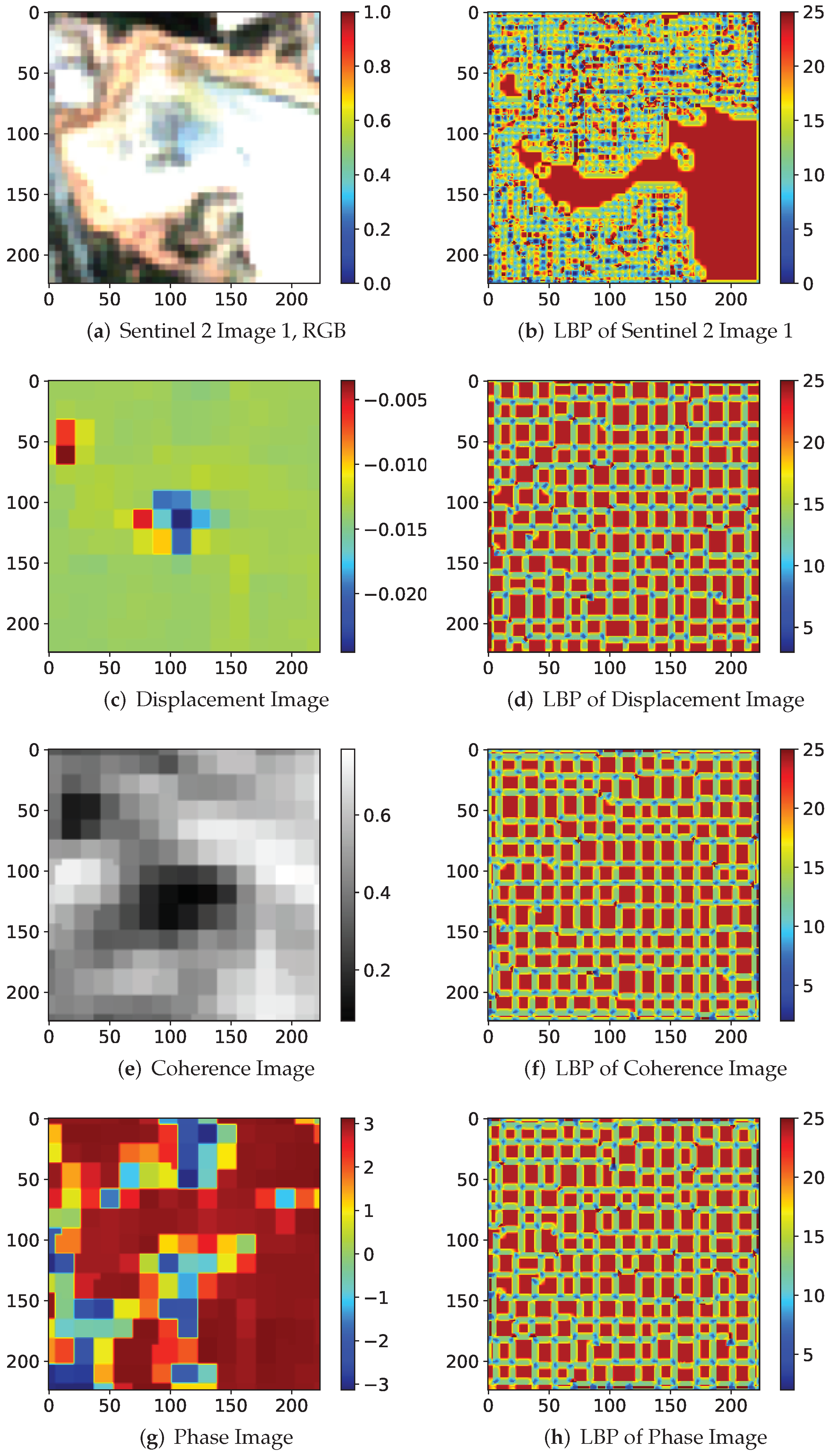
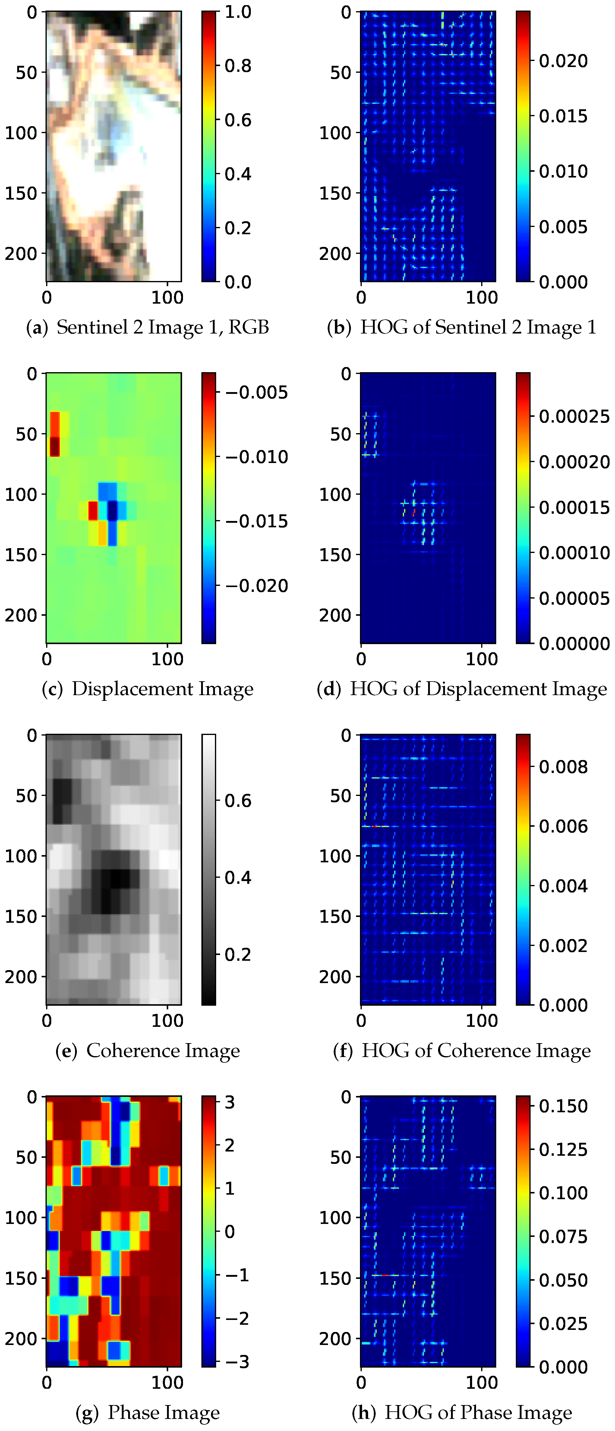
The LBP classifies textures and is commonly used in facial recognition algorithms. It is based on determining whether the points that surround the central point are greater than or less than it, and returning a result that is binary. This can then be converted into an 8-bit number [63]. The same input image sizes as those used for deep learning and used by ResNet [42] (224 × 224) are used for LBP. The two-dimensional uniform LBP is calculated using the following parameters: 24 as the number of points, i.e., eight times the radius, using a radius of three. A normalized histogram of the LBP image is generated. The HOG feature descriptor requires the input images to be resized to a 1:2 aspect ratio. To implement this, the images are resized to 112 × 224 pixels. The parameters of the HOG feature descriptor used are as follows: an 8 × 8-pixel cell window, nine orientations, and 2 × 2 cells per block. The features are also normalized in the LBP space. Both feature descriptors are applied to the phase maps, coherence maps, displacement maps, and the RGB optical image, separately. The feature vector obtained from applying the respective descriptor to each of these images, was also concatenated into a combined feature vector for a combined model. An example of the LBP and HOG feature descriptors applied to a positive blob at the location (−26.2204906351649, 28.0539217476939) are illustrated in Figure 4 and Figure 5, respectively.

2.7. Experimental Design

A balanced binary classification dataset comprising 1440 blobs (720 positive and 720 negative) was created, as described in previous sections, to compare model accuracy. The binary classification was implemented using non-deep machine learning approaches with feature extractors, classical deep learning using random initialization, and transfer learning models. In order to assess and compare model generalization and to set hyperparameters, the following protocol was followed.
Each of the sub-networks in the pair of networks use an independent neural network with identical architecture and embedding feature space length. As a result, both the RGB and the SAR data were equally weighted in the final concatenated feature vector. However, since the Sentinel-2 data contains significantly more information due to the higher resolution pixels, these would contribute somewhat more to the final classification. To this end, we performed some investigative analyses and found that the models did perform better when the Sentinel-1 and Sentinel-2 data were combined.
The dataset was split into a training set of 80% and a completely held-out testing set of 20%. The held-out set was only used for reporting the generalization accuracy and other metrics. The 80% training set was used for both hyperparameter tuning and to replicate the experiment by training multiple models for a more robust estimate of model accuracy.
For hyperparameter tuning, the parameters were obtained by using ten-fold cross-validation on the 80% training set. Ten-fold cross-validation was also employed to replicate the experiment to report expected accuracy and variance. For replication, we used nine of the ten folds from the 80% training set to fit a model and report the model accuracy on the 20% held-out set. This process of selecting nine of the ten folds was repeated ten times, with each iteration leaving out a different single fold. This process was repeated twice using different seed values when choosing the data splits to ensure increased robustness in estimating of model accuracy.
The average test accuracy results were measured. To quantify the classifier performance, the average Precision (positive predictive value), recall, and F1 score were also measured [4,66]. In order to control for family-wise error resulting from multiple comparisons, we employed the Holm Šidák correction, which has more power than other approaches. We selected an alpha level at 0.05 for family-wise significance. This protocol for multiple testing correction was appropriate as we use a completely held-out set for testing [67].

3. Results

3.1. Candidate Selection

The Laplacian of Gaussian [60] blob detection algorithm detected blobs that were both true-positives as well as false-positive blobs. The blob detection algorithm detected true-positive blobs due to changes in construction developments, quarries, highways, mines, residential complexes, and factories with parking lots. Trees, grass, crops, and other (vegetated areas) cause undesirably low coherence, which causes false-positive blobs. The blob detection algorithm also detected false-positive blobs due to water bodies, such as lakes, ponds, a green liquid at the top of mine dumps due to water having mixed with the contents of the mine dump and other water bodies [1,4].

3.1.1. True-Positive Blobs

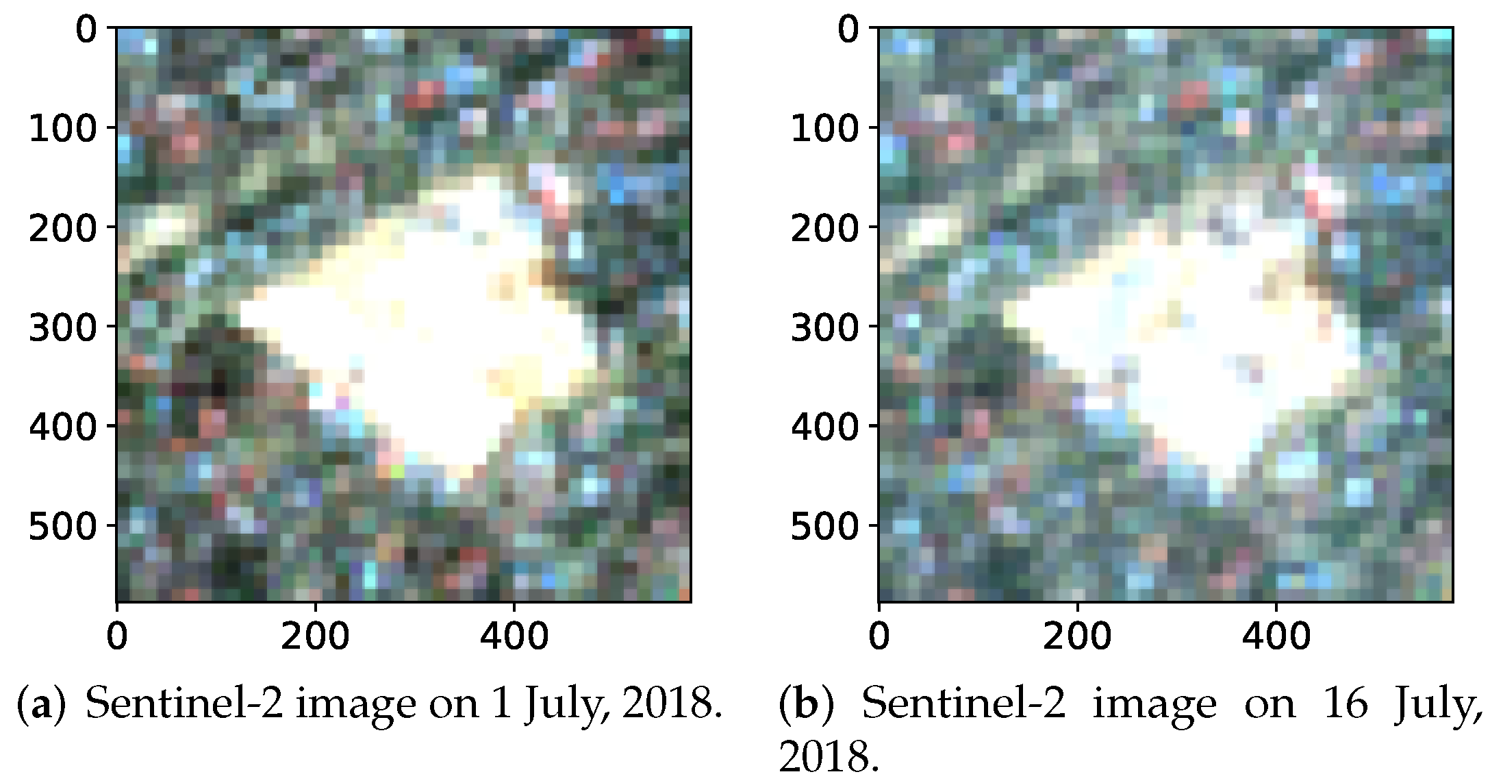
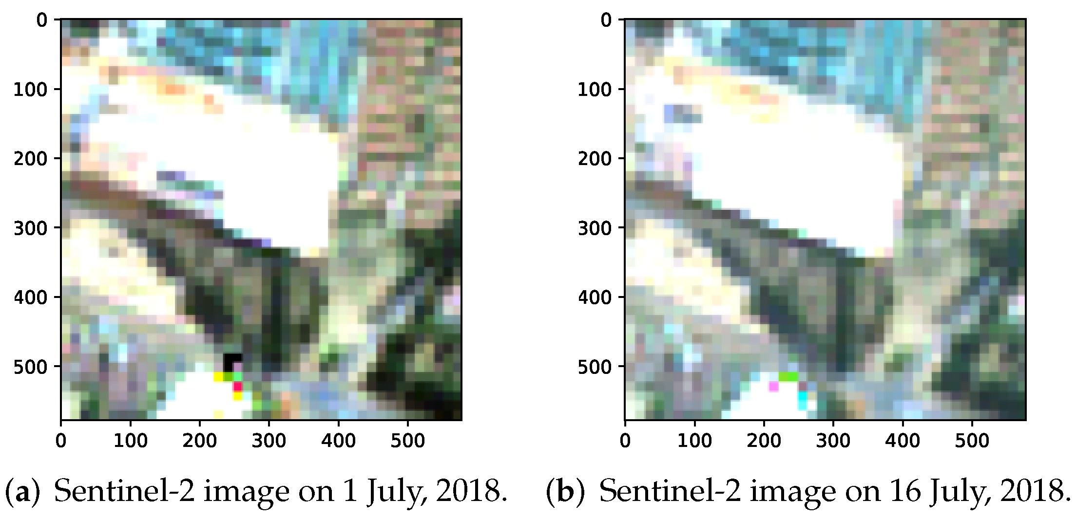
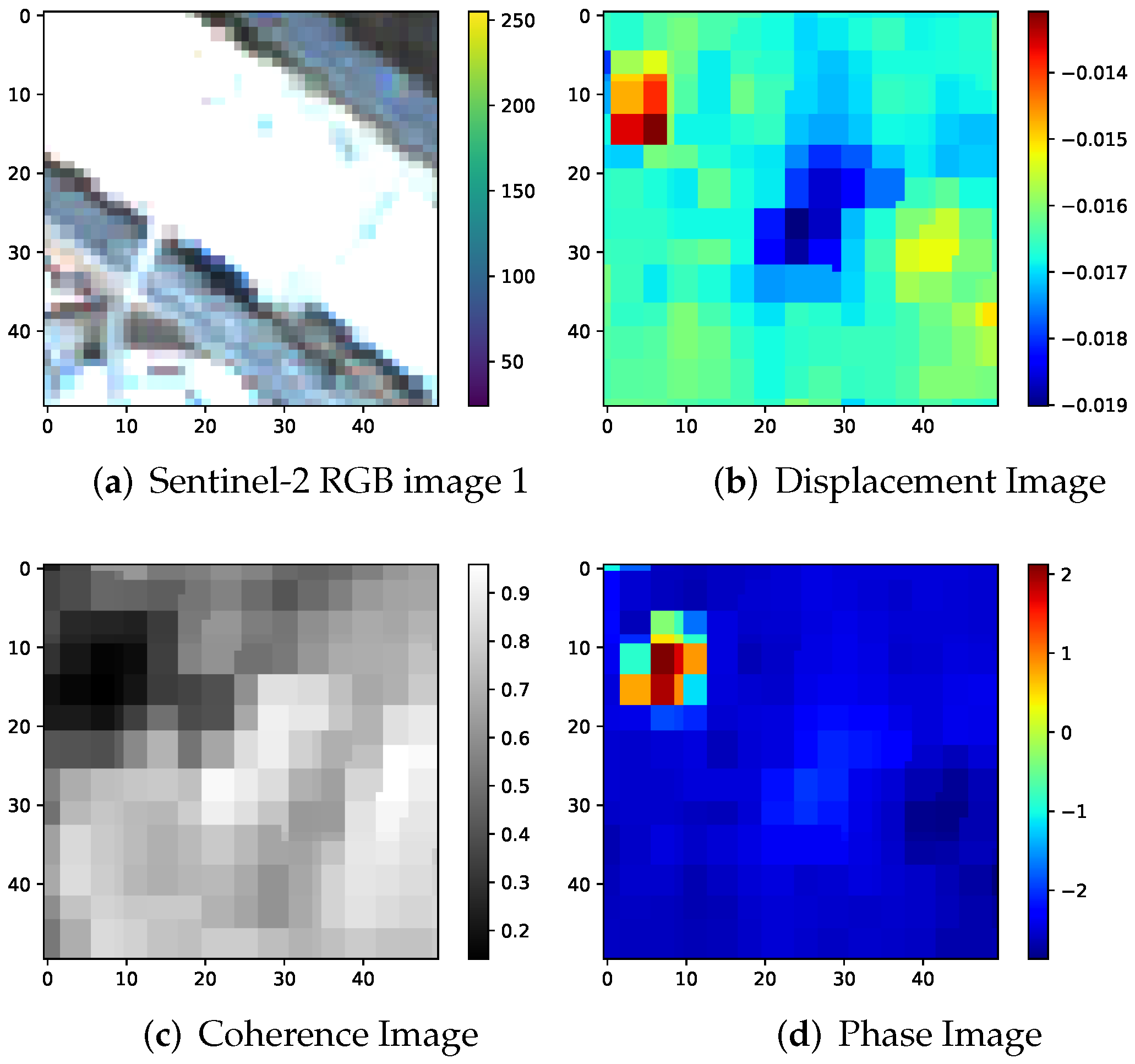
True-positive blobs are blobs where change was detected. Figure 6 shows two Sentinel-2 optical images at a 10 m resolution of an example of a true-positive blob due to construction having occurred at the coordinates (−26.1431583848774, 28.1765660900992) in Germiston, Gauteng, South Africa.
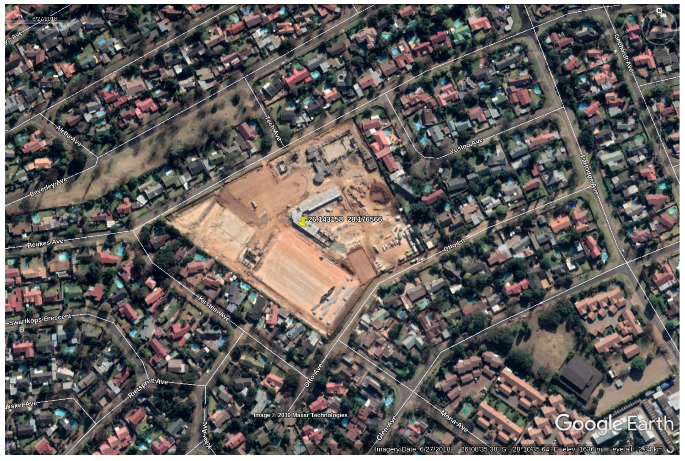
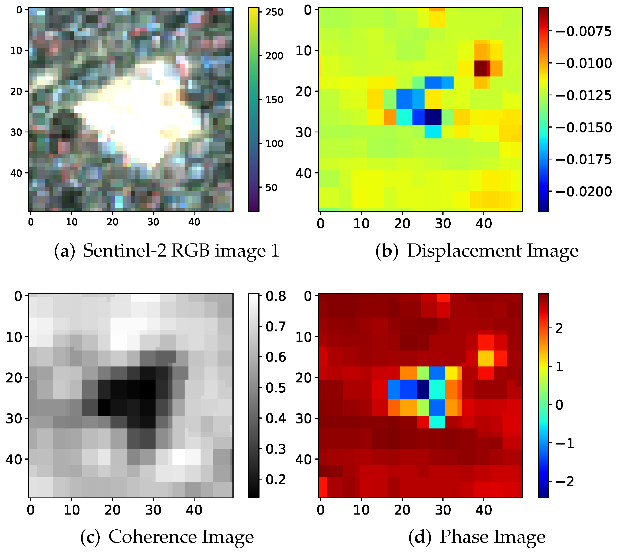
Figure 7 shows the corresponding Google Earth [62] image on 27 June 2018, confirming that it is a construction site as the construction of the roof of the building is visible. Figure 8 illustrates the true-positive blob’s corresponding DInSAR processed phase, coherence, and displacement maps with the corresponding Sentinel-2 RGB image.
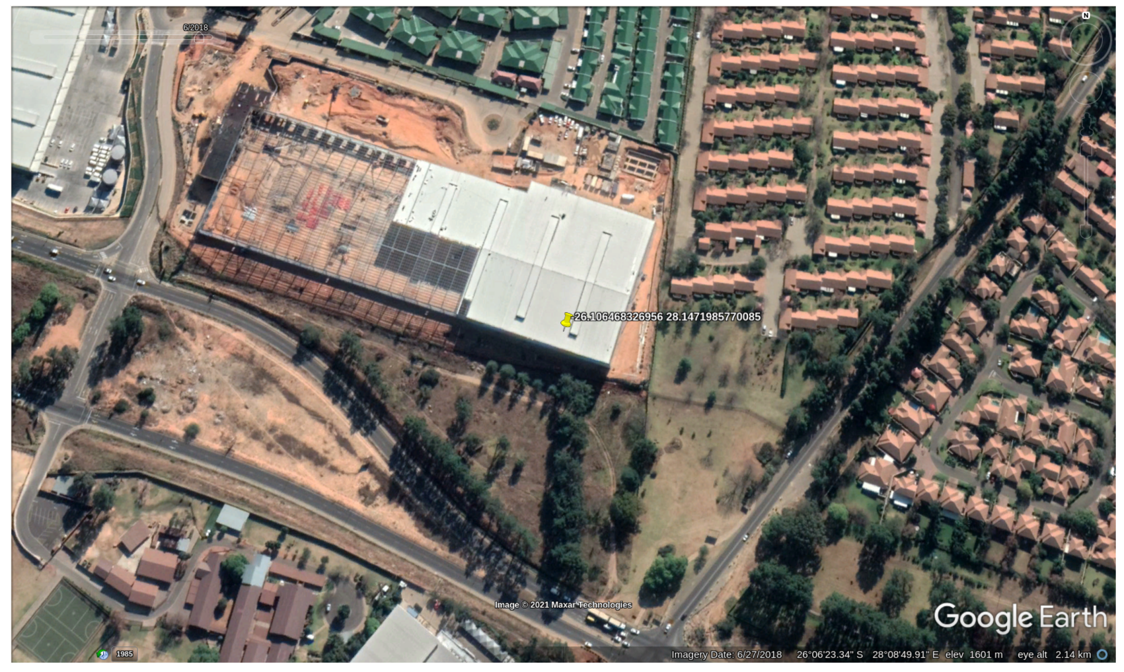
Figure 9 shows the two Sentinel-2 optical images of a true-positive blob with construction at the coordinates (−26.106468326956, 28.1471985770085) in Thornhill Estate, Gauteng, South Africa. Figure 10 shows the corresponding Google Earth [62] image in June 2018, confirming that it is a construction site.
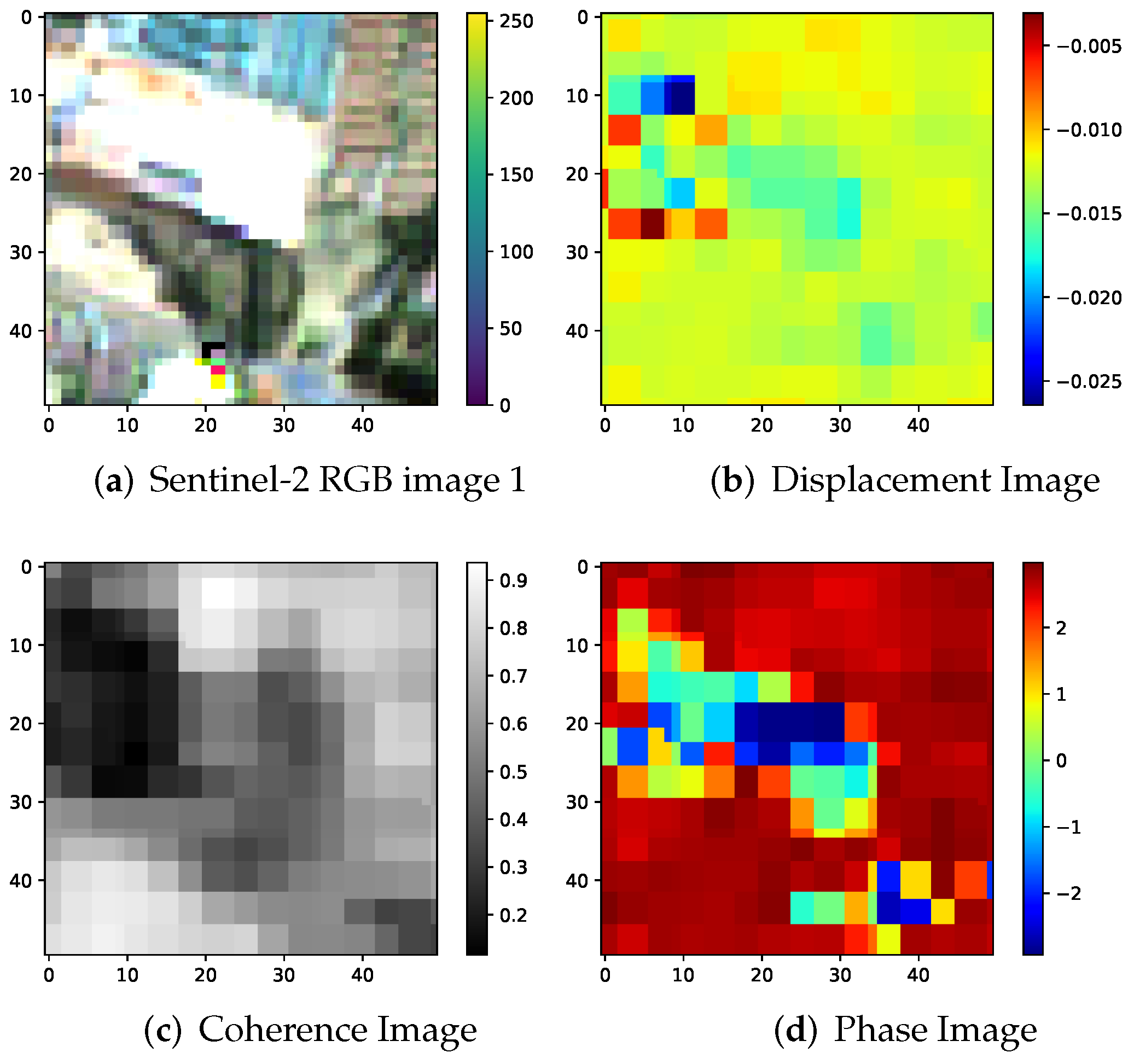
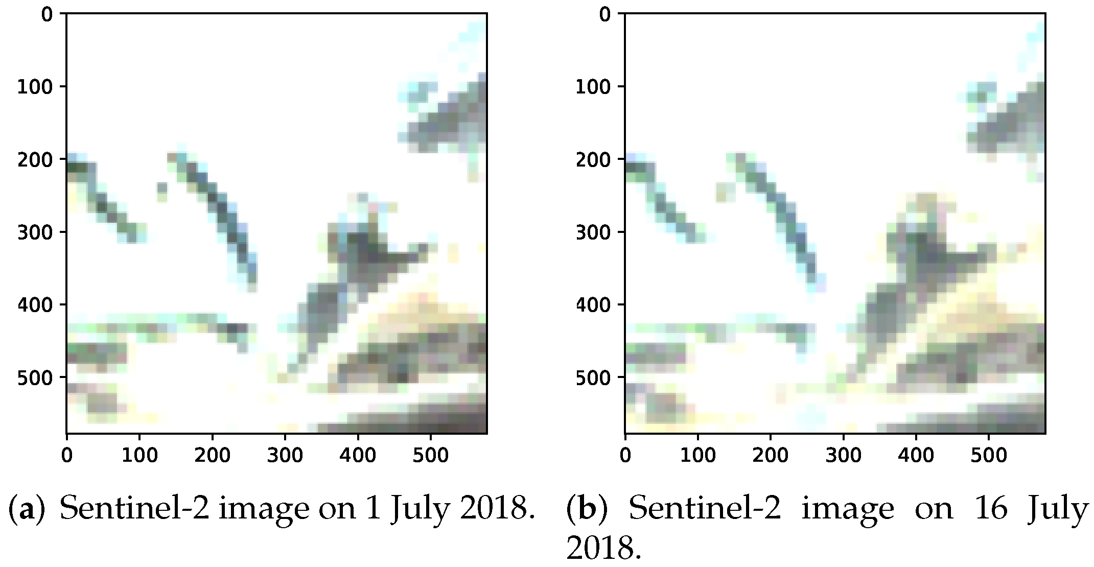
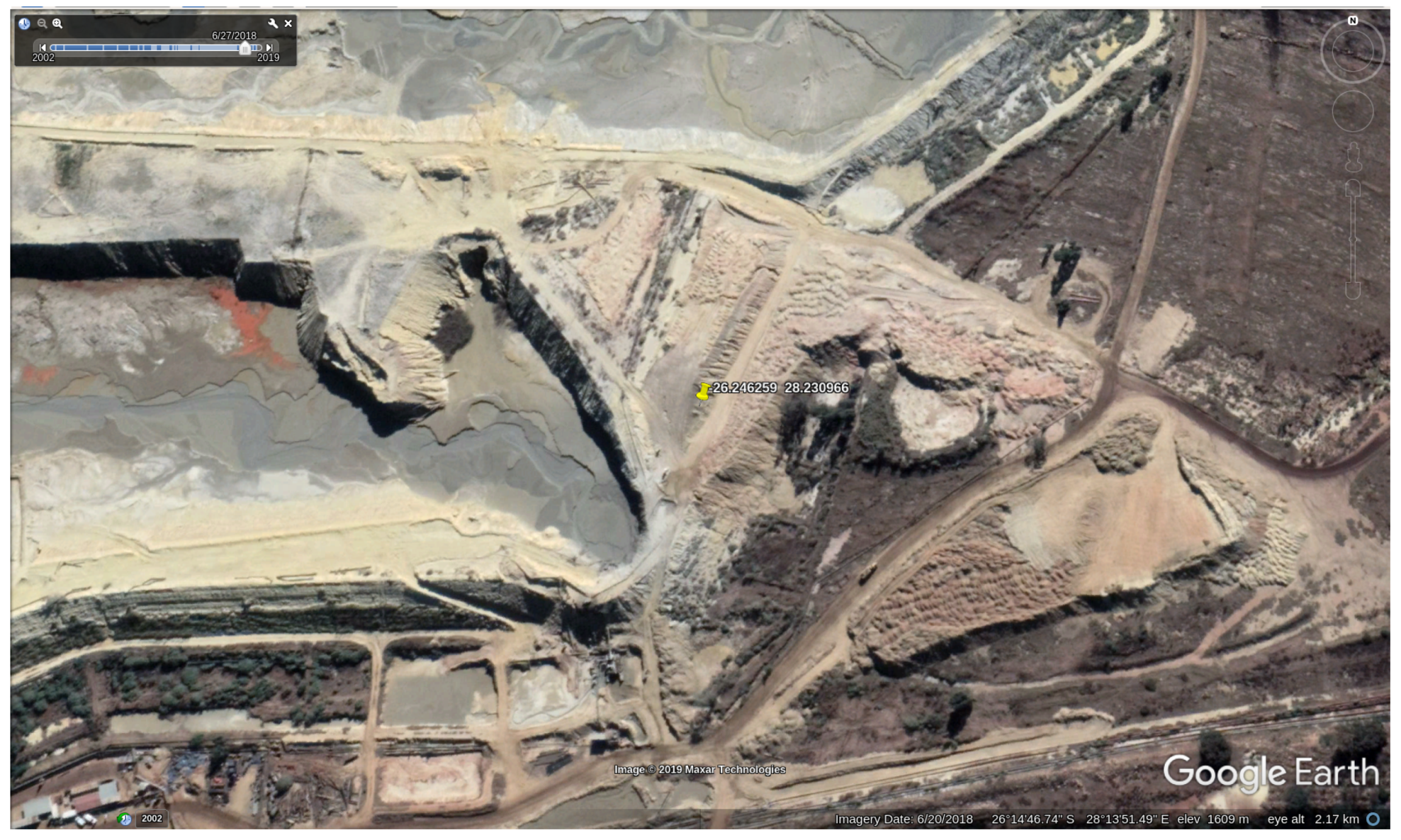
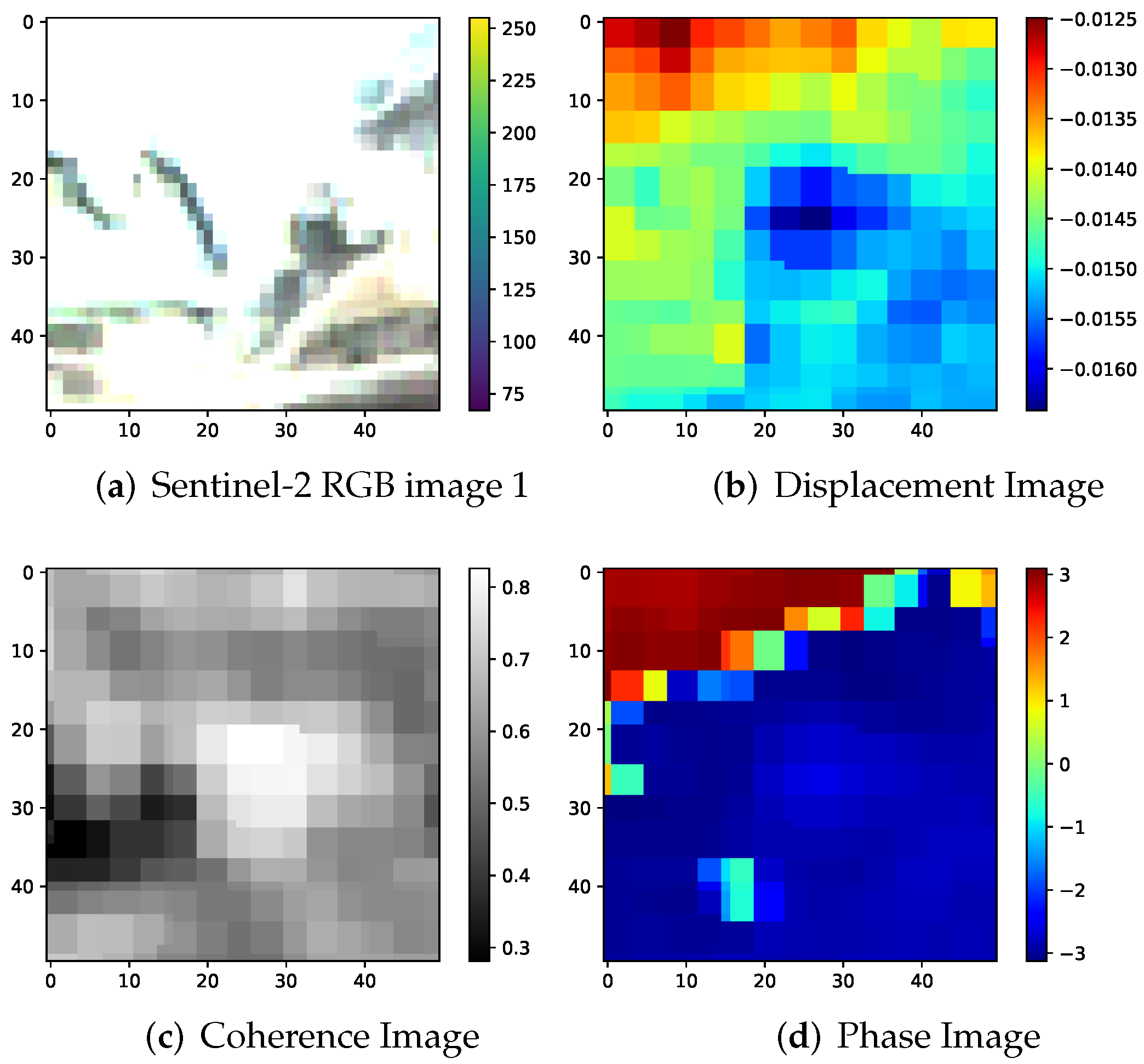
Figure 11 illustrates the true-positive blob’s corresponding DInSAR processed phase, coherence, and displacement images with corresponding Sentinel-2 RGB image. Figure 12 shows the two Sentinel-2 optical images of a true-positive blob at a gold surface mine dump tailings retreatment facility (Elsburg Tailings Complex) at the coordinates (−26.2462588162865, 28.230965774735) in Boksburg, Gauteng, South Africa.
Figure 13 shows the corresponding Google Earth [62] image on 27 June 2018, confirming that it is a tailings mine dump retreatment facility. Figure 14 illustrates the true-positive blob’s corresponding DInSAR processed phase, coherence, and displacement images with corresponding Sentinel-2 RGB image.
Figure 15 shows the two Sentinel-2 optical images of a true-positive blob at a factory yard containing trucks and containers at the coordinates (−26.2482935080064, 28.1374744753349) in Alberton, Gauteng, South Africa. Figure 16 shows the corresponding Google Earth [62] image on 27 June 2018, confirming that it is a factory yard with containers and trucks whose movement would correspond to the change detected. Figure 17 illustrates the true-positive blob’s corresponding DInSAR processed phase, coherence, and displacement images with corresponding Sentinel-2 RGB image.

3.1.2. False-Positive Blobs

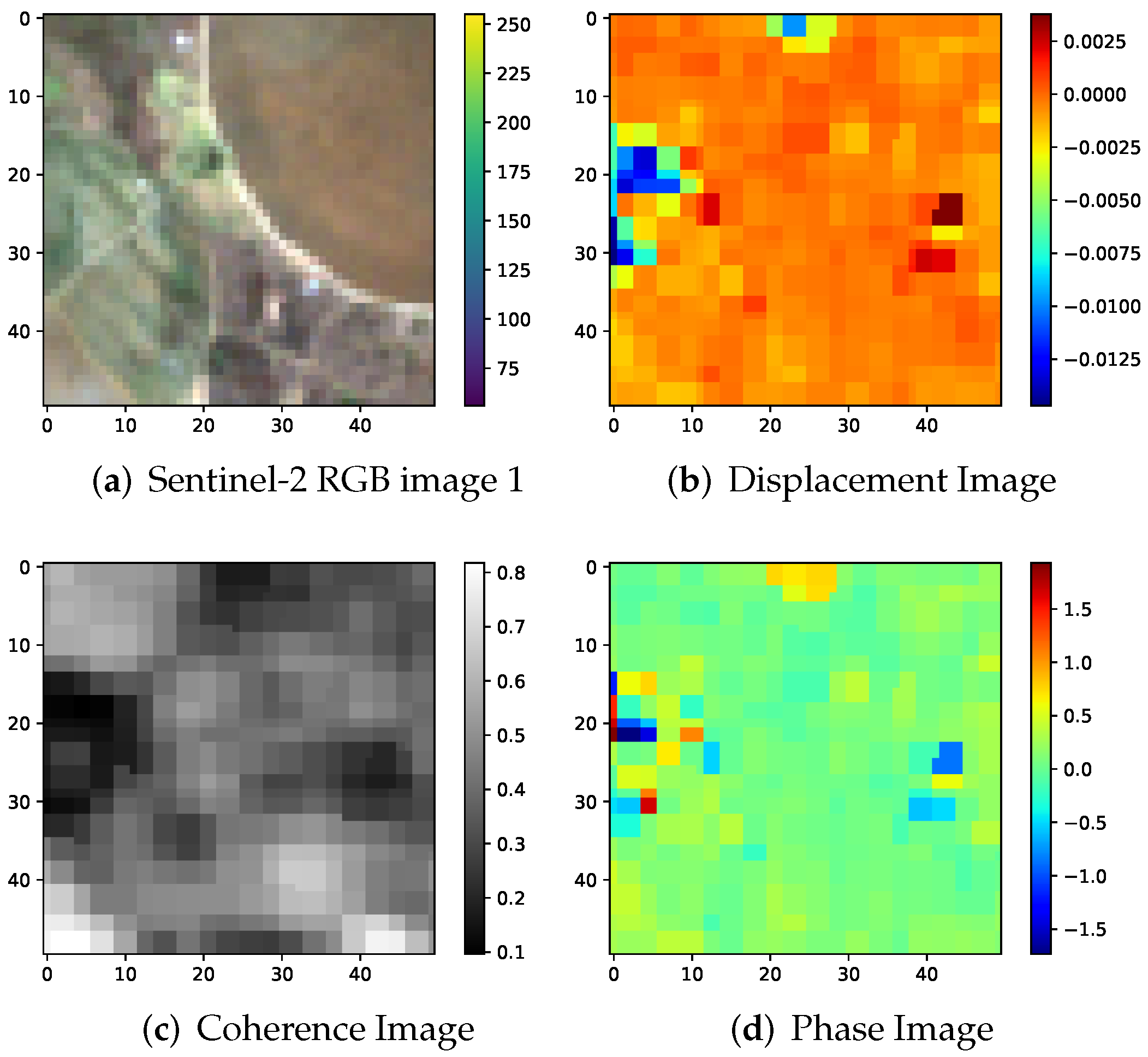
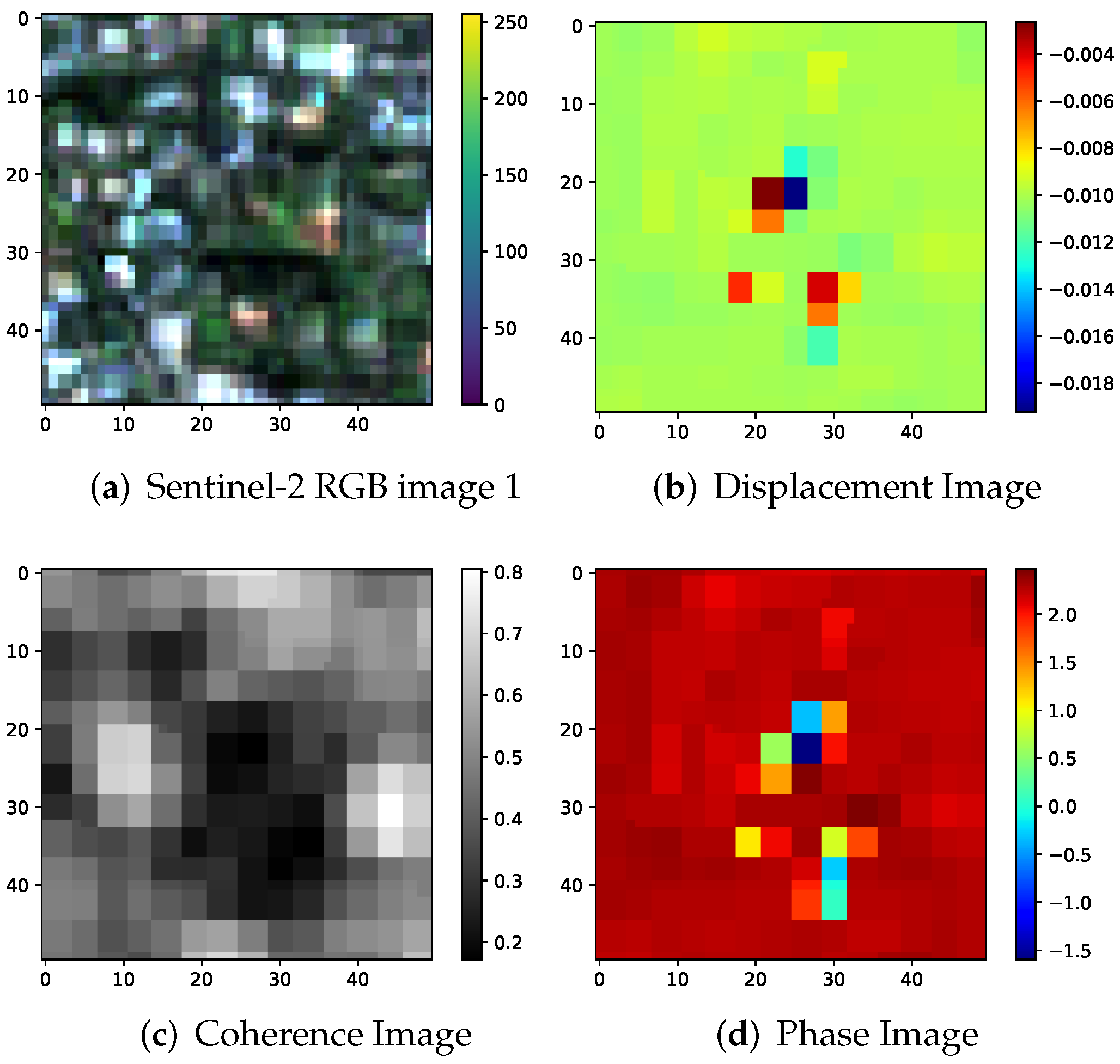
False-positive blobs are blobs identified by the blob detection algorithm where industrial change has not occurred, but are actually as a result of bad coherence due to artifacts in the interferogram. These are used as the negative samples in binary classification.
Figure 18 shows the two Sentinel-2 optical images of a false-positive blob due to vegetation causing a blob as a result of the bad coherence at the coordinates (−25.5669752259105, 28.2160704977751) in Pretoria Rural, Gauteng, South Africa. Figure 19 illustrates the false-positive blob’s corresponding DInSAR processed phase, coherence, and displacement images with corresponding Sentinel-2 RGB image.
Figure 20 illustrates the DInSAR processed phase, coherence, and displacement images with the corresponding Sentinel-2 RGB image of a false-positive blob that was caused by trees (vegetation), causing undesirably low coherence at the coordinates (−26.1241380519143, 28.0437540461661) in an urban area in Hyde Park, Gauteng, South Africa.
The decision boundary between true-positive blobs (used as positive samples in binary classification) and false-positive blobs (used as negative samples for binary classification) is not distinctly defined, as both can occur when there is undesirably low coherence and also when there is good coherence.

3.2. Binary Classification

Table 2, Table 3, Table 4, Table 5, Table 6 and Table 7 contain the experimental performance results that were achieved [1,4]. We highlight the best performing methods in bold. We also highlight, in gray, the methods that are not significantly different from the best performing method using a two-sided t-test at p 0.05 with the alternate hypothesis being that the best performing method is greater.
Table 2 contains the results of the deep learning and transfer learning single models. ResNet50 has the best performance followed by ResNet101, which is not statistically significantly different from ResNet50.
In Table 3 the results of the FeatSpaceEnsNets are contained. All of the FeatSpaceEnsNets, except for FeatSpaceEnsNet 5, outperform the best performing single model, ResNet50, showing the value of the feature space ensembles. Table 4 presents the results of the AvgEnsNets, five of which have better performances than the best-performing ResNet50 model. We note that the top five AvgEnsNets are not statistically significantly different.
To evaluate if the use of a hybrid approach would further increase upon the FeatSpaceEnsNet and AvgEnsNets, we turn to Table 5, which has the results of the HybridEnsNets. The best-performing HybridEnsNets do not outperform the best AvgEnsNet, but none are statistically significantly different.
Finally, we compared the results of the best of each of the FeatSpaceEnsNets, AvgEnsNets, and HybridEnsNets against our ConvNet2, and some non-deep machine learning approaches. From Table 6, we note that AvgEnsNet 7 is the best-performing model; however, it is not statistically significantly better than the other ensembles.

3.3. Effect of Varying Cross-Validation Folds

Table 7 contains the results of the best performing models from each class of method, decision tree ensemble: LBP-RF, linear: LBP-SVM, non-linear-shallow: LBP-RBF-SVM, non-linear-deep: ResNet50 and non-linear-deep-ensemble: AvgEnsNet 7 and FeatSpaceEnsNet 2 under ten, five and two cross-validation folds. The results when using five-fold cross-validation indicate a slight drop in performance as compared to when using ten fold cross-validation. The local binary pattern model with a radial basis function SVM classifier had a more pronounced drop of 1.5% when using five-fold instead of two-fold cross-validation. However, when using two-fold cross-validation most of the models evaluated have better performance than when using five-fold or ten-fold cross-validation. This is due to there being more training data when using two-fold cross-validation. Only the local binary pattern model with a radial basis function SVM classifier has slightly worst performance when using two-fold cross-validation compared to using ten-fold cross-validation. Ten-fold cross-validation has a higher F1 score for all the models except for the LBP with a linear SVM classifier model.

3.4. Visualization of Results

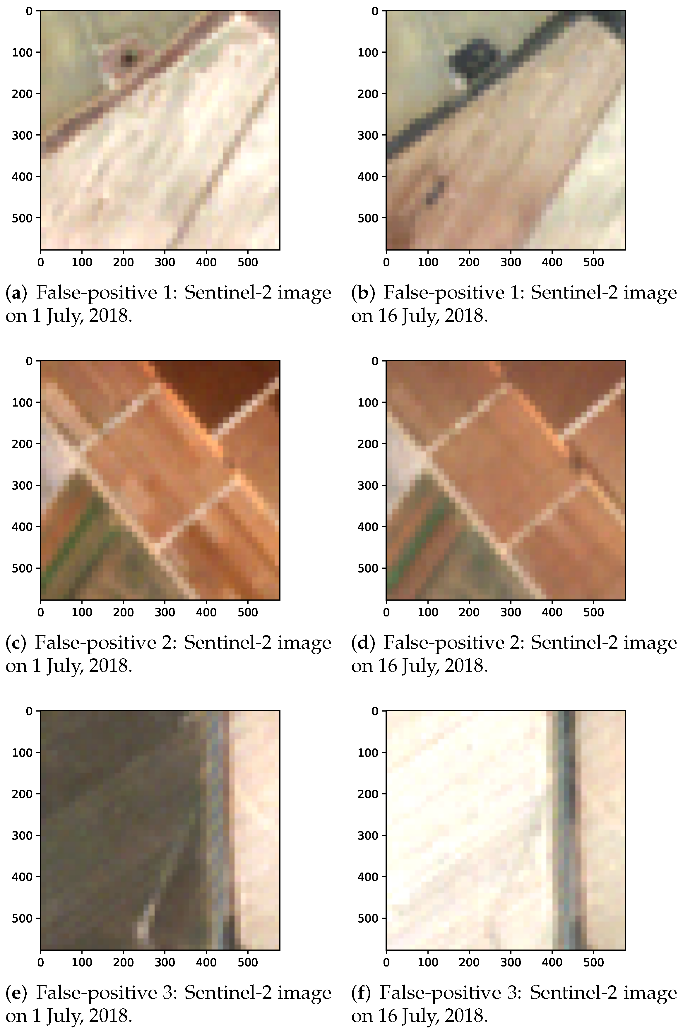
Figure 21 shows the two Sentinel-2 optical images of four of the false-positive blobs that the best performing classifier (AvgEnsNet 7) incorrectly classified. False-positives tend to occur over vegetated areas containing crops, trees, etc.
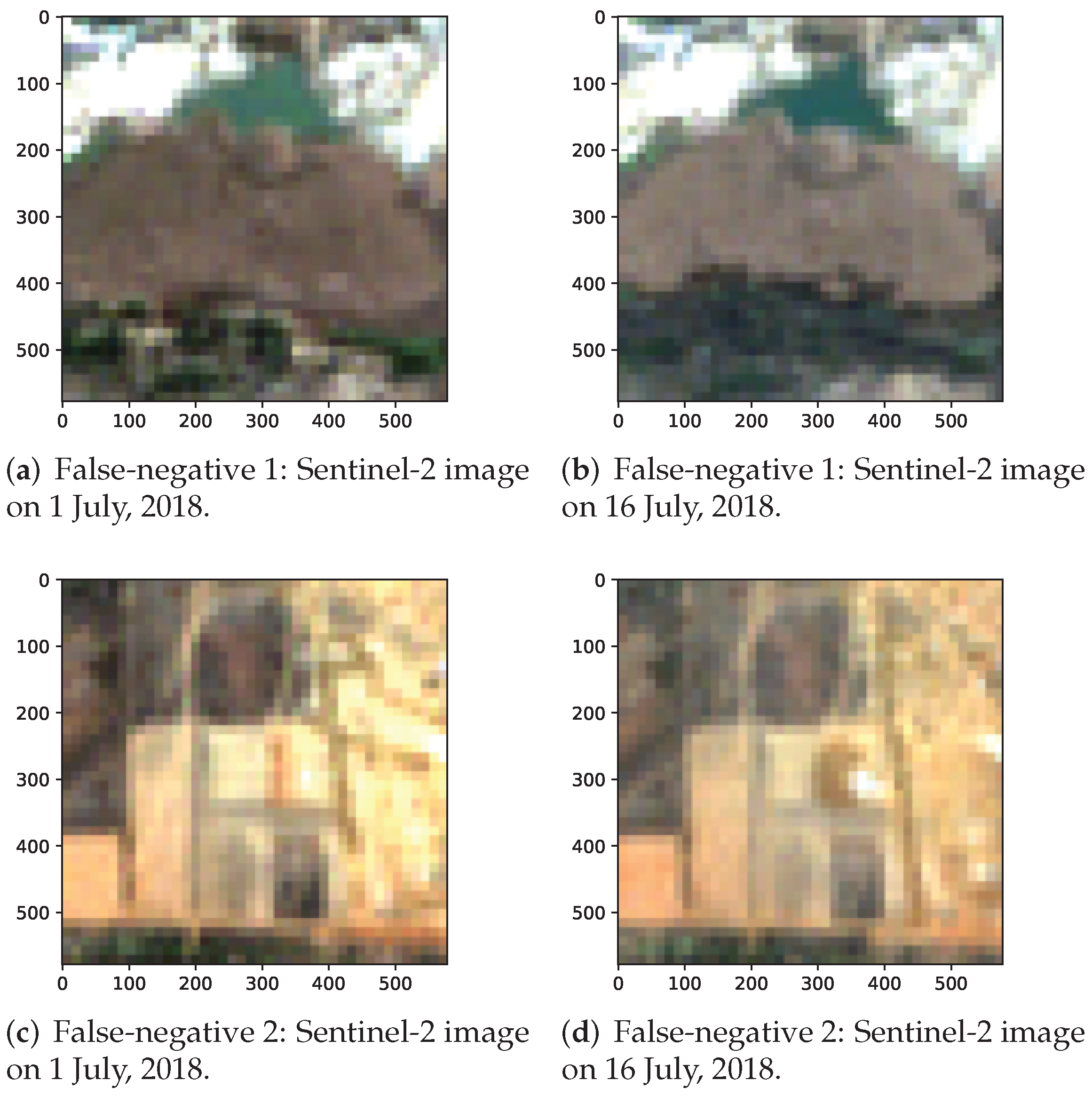
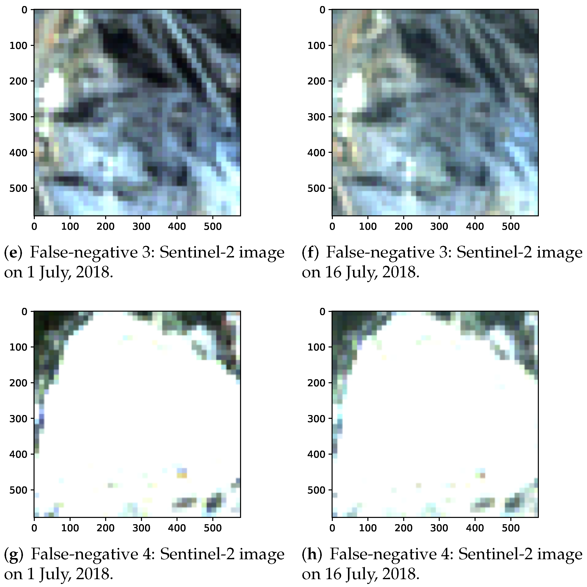
Figure 22 shows the two Sentinel-2 optical images of four of the false-negative blobs that the best performing classifier (AvgEnsNet 7) incorrectly classified. False-negatives tend to occur where there are partial images of construction sites in the image together with vegetated land, as in False-negative 1 and 2. False-negative 3 and 4 also show partial images, which contain vegetated land, together with quarries in the images.

4. Discussion

4.1. Non-Deep Machine Learning: LBP and HOG with Linear SVM, Radial Basis Function (RBF) SVM, Random Forest (RF), and Multi-Layer Perceptron (MLP) Neural Network

The average testing accuracy performances achieved when using the LBP and HOG feature extractors on their own, and using their combination with a linear support vector machine (SVM), radial basis function SVM, random forest, and multi-layer perceptron classifiers are contained in Table 6. The models with LBP had better performance than the models with HOG or their combination (HOG, LBP) used as a feature extractor. The uniform LBP RBF-SVM (70.522%) outperforms all of the other classifiers that use the LBP, HOG, and their combination feature extractors. All of the LBP classifiers also performed better than the EfficientNet B4 model used with DLRI (65.608%) from Table 2. This result can be attributed to the dataset being small and the fact that there are a large number of parameters that DNNs require to be adequately trained for them to achieve high-performance results when performing DLRI. However, ResNet50 with DLRI and TLFT outperformed all of the non-deep machine learning models, so there is variation when considering architecture. The LBP with RBF-SVM (70.522%) and LBP with random forest classifiers (69.896%) also outperform the EfficientNet B4 model used with TLFT (67.881%). However, all of the TLFE DNN architectures outperformed all of the non-deep machine learning models considered [4].

4.2. ConvNet2

The two-layer CNN, ConvNet2, acquired an average test accuracy performance of 82.640%. Despite having a straightforward architecture, it performed better than most of the single models. Only the ResNet50, ResNet101, and Inception-ResNetV2 architectures with TLFE and the ensemble models performed better than ConvNet2. It achieved a performance of only 1.111% less than the ResNet50 architecture using TLFE, which had the best single model performance. This result can also perhaps be attributed to the dataset being small. Due consideration must also be given to the fact that the ConvNet2 model was trained from scratch on this dataset, which also included DInSAR processed band images of phase, coherence, and displacement and Sentinel-2 optical imagery that are not at all similar to any of the classes of images that the transfer learning models were trained on in the ImageNet dataset. Despite this fact, transfer learning with the ResNet50, ResNet101, and Inception-ResNetV2 single model architectures, and the ensemble models outperformed the ConvNet2 and the classic ML baseline. ConvNet2 leverages modern advancements in regularization to combat overfitting; thus, it is not similar to the classic artificial neural networks (ANN) or CNNs that used fully connected layers and suffered from overfitting and need large amounts of data to be trained. ConvNet2 has dropout, batch normalization and global average pooling layers. These modern advancements increase its ability to generalize and perform better on unseen data [4].

4.3. Transfer Learning by Feature Extraction

From all of the single models, TLFE with the ResNet50 and TLFE with the ResNet101 both individually outperform all of the other single models, which includes newer architectures, such as ResNeXt50, EfficientNet, ResNetV2, and Inception-ResNetV2. The mean test accuracy of TLFE with ResNet50 (83.751%) outperforms the mean test accuracy of TLFE with ResNet101 (83.403%) by 0.348% despite ResNet101 being a deeper network with 101 layers and ResNet50 having only 50 layers [1,4]. ResNet50 is the best performing single model with an accuracy of 83.751%. ResNet50 used as a feature extractor for transfer learning also outperformed all of the non-deep machine learning models, such as the LBP and HOG feature descriptors and their combination with Linear SVM, RBF-SVM, RF, and MLP classifiers. ResNet50 also outperforms ConvNet2 by 1.110% [4].
The power of ensembling, combined with TLFE, is demonstrated by the fact that all of the ensembles evaluated using TLFE have a mean accuracy of at least 83.472% and an F1 score of at least 0.836. The EfficientNet family of models that were evaluated with TLFE reaches its peak performance using the EfficientNet B0 architecture (82.221%). It has a performance of 1.180% higher than the performance achieved by the deeper EfficientNet B4 architecture (81.041%). Even though EfficientNet B0 is the shallowest network (5 m parameters), it still attains a noteworthy performance (82.221%), which is also higher than the much deeper EfficientNet B7 (79.688%) and also higher than the ResNet152’s performance (80.677%). This result is observed even though these much deeper networks have 13 × and 12 × more parameters, respectively.
FeatSpaceEnsNet 2 (comprised of ResNet50, ResNeXt50, and EfficientNet B4) outperforms all of the AvgEnsNet and HybridEnsNet models except for AvgEnsNet 7. FeatSpaceEnsNet 2 (84.862%) achieved a mean test accuracy percentage of only 0.087% more than what HybridEnsNet 3 (84.775) achieved. Since FeatSpaceEnsNet 3 only contains three models and is a much simpler ensemble model than HybridEnsNet 3 (which contains eight models of different model types and also includes FeatSpaceEnsNet 3), but does not outperform FeatSpaceEnsNet 2, this is a significant result. Considering the quantity of models contained in the ensemble, FeatSpaceEnsNet 2 only has 37.5% of the number of models that HybridEnsNet 3 has. FeatSpaceEnsNet 2 also only has effectively 70 m parameters compared to HybridEnsNet 3, which leverages the benefits of effectively 245 m parameters. Thus, FeatSpaceEnsNet 2 has a parameter size that is 28.571% of the parameter size of HybridEnsNet 3 since the single models do not have the same number of parameters. FeatSpaceEnsNet 2 also has a narrower mean accuracy variance than HybridEnsNet 3. FeatSpaceEnsNet 2’s F1 score is 0.001 more than the F1 score of HybridEnsNet 3.
From the seven models, which achieved a mean test accuracy percentage greater than 84.5%, HybridEnsNet 2 has the most negligible variance (0.794), which is 57.787% of the variance of AvgEnsNet 7. HybridEnsNet 2 achieved an F1 score of 0.847, which is 99.647% of the F1 score of the top-performing model, which was 0.850. All of the AvgEnsNet models evaluated outperform the best single model, ResNet50 with TLFE, except for AvgEnsNet 3 and AvgEnsNet 6. Five of the seven FeatSpaceEnsNets that have a similar composition to the respective AvgEnsNets have a higher performance than the corresponding AvgEnsNet models. FeatSpaceEnsNet 7, FeatSpaceEnsNet 3, FeatSpaceEnsNet 1, FeatSpaceEnsNet 4, and FeatSpaceEnsNet 5 outperformed the corresponding similarly composed AvgEnsNets, AvgEnsNet 1, AvgEnsNet 2, AvgEnsNet 3, AvgEnsNet 4, and AvgEnsNet 6, respectively. Only AvgEnsNet 5 outperformed its corresponding FeatSpaceEnsNet, FeatSpaceEnsNet 6. AvgEnsNet 7 has the same mean accuracy performance as its corresponding FeatSpaceEnsNet, FeatSpaceEnsNet 2, but has an F1-score that is higher by 0.001 and a variance that is wider by 0.266. In general, AvgEnsNets are computationally simpler to train since the size of the combined feature vector increases with an increase in the number of models in the ensemble, which consequently increases the complexity and the training time it takes to fit a single Logistic Regression model to the large combined feature vector.

4.4. Transfer Learning by Fine-Tuning and Deep Learning from Random Initialization

The DLRI mean accuracy performance is 9.773% higher than the fine-tuning mean accuracy performance for the ResNet50 model. Transfer learning via feature extraction with ResNet50 outperformed both DLRI and TLFT with ResNet50 by 2.900% and 12.673%, respectively. This result is probably due to there not being enough data to adequately train the model, since both random initialization and TLFT need two models, which are combined in the final layer. Transfer learning by feature extraction, on the other hand, requires no actual training. EfficientNet B4 with TLFE (81.041%) performed better than both DLRI (66.608%) and also better than fine-tuning (67.881%), respectively.
All of the single models that used TLFE outperformed classic deep learning and the fine-tuning method of transfer learning with the EfficientNet B4 architecture. All of the single models that used TLFE also outperformed fine-tuning with the ResNet50. This observation correlates with the literature as it is mentioned by Kornblith et al. [18] that TLFE performs better for smaller datasets than TLFT [1,4,18]. If a much bigger dataset was available, then DLRI would perform better than transfer learning in general. A crucial parameter in determining whether classic deep learning or transfer learning performs better is the size of the dataset. Another factor that affects transfer learning performance is the similarity of the dataset that the model was trained on to the target dataset [4,18].
ResNet50 DLRI, classic deep learning, has a mean accuracy performance (80.851%) that is 15.243% better than that of EfficientNet B4 (65.608%) on this small dataset despite ResNet50 having seven million more parameters. ResNet50 DLRI also outperformed TLFE with ResNet152, EfficientNet B7, ResNet152V2, and ResNet50V2. ResNet50 DLRI also outperformed TLFT with ResNet50. ResNet50 fine-tuning has a 3.197% higher accuracy than EfficientNet B4 fine-tuning, even though the EfficientNet architecture was designed using the neural architecture search, which leverages machine learning to acquire the best architecture configuration, which optimizes ImageNet performance [1,4,51].
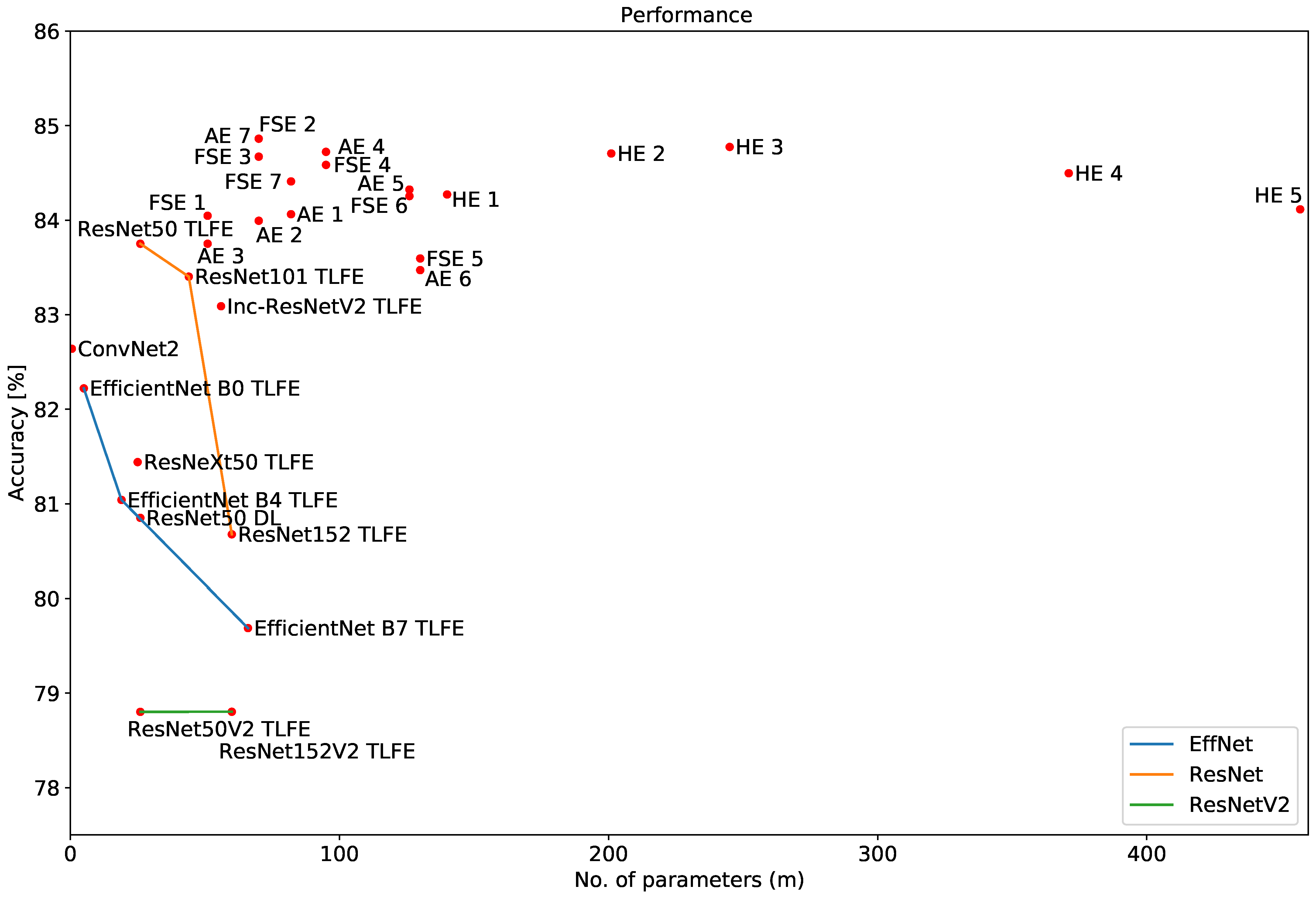
Figure 23 illustrates the average test accuracy concerning parameter size. A trend line is shown for models from the same architecture. The ResNet results are shown in orange. Using a model with more layers decreases the single model performance. There is a steep decrease in performance between feature extraction done using the ResNet101 model and the ResNet152 single model. This decrease in performance is steeper than the decrease in performance observed between the ResNet50 and ResNet101 models. This result is observed despite the increase in the number of parameters (18 m) being less when comparing the ResNet50 model (26 m) to the ResNet101 model (44 m) than the increase in the number of parameters (16 m) when comparing the ResNet101 (44 m) model to the ResNet152 model (60 m). For the EfficientNet architecture (shown in blue), a decrease in performance with an increase in the number of parameters in the model is also observed. For the ResNetV2 architecture, the line indicating performance observed is almost horizontal when comparing the performance of the ResNet50V2 model to the performance of the deeper ResNet152 model with 102 more layers. The number of parameters of the ResNet50 (version 1) and the ResNet50V2 models is the same and the number of parameters of the ResNet152 (version 1) and ResNet152V2 models is also the same. However, the steepness of decrease in performance comparing the ResNet50 model (50-layer ResNet) to the ResNet152 model (152-layer ResNet) is more pronounced in the version 1 architecture, where performance decreases by 3.074%, than in the version 2 architecture, where it increases by 0.001%. An inverse correlation between mean test accuracy and deep learning network size is evident in general when the architecture remains constant.
Mean accuracy of above 78% was achieved by all models with at least 30 m parameters. Mean accuracy of at least 83.47% was achieved by all models with at least 70 m parameters. There is a non-linear correlation between the number of parameters in the model and the mean accuracy achieved in general. However, it must be noted that classic DLRI and fine-tuning have only been evaluated on: ResNet50 (26 m parameters) and EfficientNet B4 (19 m parameters). From Figure 23, it is evident that on this dataset, most of the models which used the feature extraction method of transfer learning performed better than DLRI and TLFT method with the ResNet50 and EfficientNet B4 architectures, respectively. This result was independent of parameter size. Had more DLRI been used, then due to the small size of the dataset, as compared to the millions of images in ImageNet, deeper networks would have performed worst due to not having enough data to train all the parameters [4].
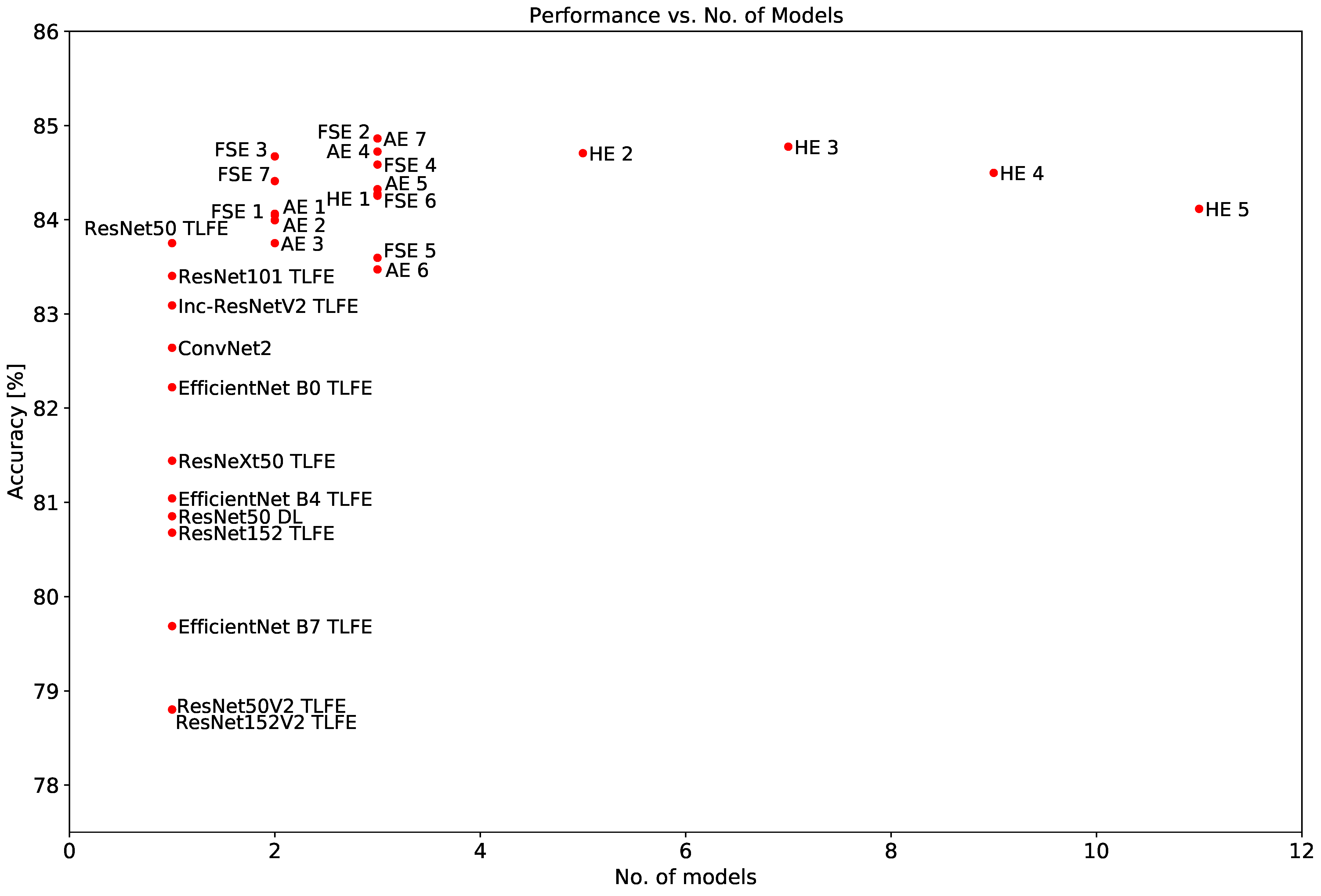
Figure 24 illustrates the average test accuracy performance concerning the number of models used. In general, single models do not perform as well as ensembles of models with more than one model. An increase in performance with an increase in the number of models in the ensemble is not observed. AvgEnsNet 7 achieves the peak performance which contains three models (ResNet50, ResNeXt50 and EfficientNet B4). A slight increase in performance accuracy percentage is observed when increasing the model number from HybridEnsNet 1 to HybridEnsNet 2 and from HybridEnsNet 2 to HybridEnsNet 3. However, a decrease in performance is observed when increasing the number of models from HybridEnsNet 3 to HybridEnsNet 4 and from HybridEnsNet 4 to HybridEnsNet 5 respectively. This is due to the addition of lower performing single models in the composition of the HybridEnsNet 4 and HybridEnsNet 5 ensembles as compared to the other HybridEnsNet models with reference to Table 1.
Figure 25, Figure 26 and Figure 27 illustrate the confusion matrix of the best performing models (AvgEnsNet 7, HybridEnsNet3, and FeatSpaceEnsNet 2) that were evaluated. FeatSpaceEnsNet 2 and HybridEnsNet 3 both have one less false-positive and one more false-negative than AvgEnsNet 7. AvgEnsNet 7 has one true-positive more than HybridEnsNet 3 and FeatSpaceEnsNet 2, respectively. AvgEnsNet 7 also has one true-negative less than HybridEnsNet 3 and FeatSpaceEnsNet 2, respectively.

4.5. Limitations

Since changes need to be at least 28 m × 34 m, the resolution of the DInSAR processed imagery also contributes to the high false-positive rate since it is skewed to detecting significant area changes. Nevertheless, true-positive blobs are detected due to mines, construction sites (uplift and subsidence), quarries, parking lots and factory yards. In cases where there is industrial infrastructure in areas where there are high rise buildings the performance may deteriorate. Only the RGB bands of Sentinel-2 are considered, adding some of the other bands may have improved performance. Only the VV polarization of the Sentinel-1 SAR data was used. The occurrence of water bodies or snow covered surfaces also leads to bad coherence and false positives being generated. However, the visual spectral information would counter this to some extent.

4.6. Complexity of the Different Approaches

DLRI trains the whole network and requires the longest training time. TLFT runs faster than DLRI since the whole network is not trained. However, TLFE has the fastest running time since no neural networks are actually trained, only a simple linear model is trained on the feature maps. ’Ensembling’ with TLFE improves the accuracy, but requires more running time to train. The more models included in the ensemble the longer the training time required. Training FeatSpaceEnsNets is more computationally expensive than training AvgEnsNets and has a longer running time since only one logistic regression model is trained on the concatenated feature vector, which is much larger than the individual feature vectors. The AvgEnsNets are also more computationally faster than the HybridEnsNets due to them including one FeatSpaceEnsNet and a larger number of single models.

5. Conclusions

A novel dataset was developed comprising Sentinel-2 optical RGB images fused with the corresponding Sentinel-1 DInSAR coherence, phase and displacement maps for binary classification for industrial change detection. The knowledge learnt from the ImageNet RGB images dataset was transferred to the novel dataset. All of the models that used TLFE outperformed classic deep learning and the fine-tuning method of transfer learning with the EfficientNet B4 architecture and they also outperformed fine-tuning with ResNet50. This is due to the small size of the dataset limitation which prevents the adequate training of DNNs. From all of the single models, TLFE with the ResNet50 and TLFE with the ResNet101 both individually outperform all of the other single models, which include newer architectures, such as ResNeXt50, EfficientNet, ResNetV2, and Inception-ResNetV2. ResNet50 is the best performing single model with an accuracy of 83.751%. ResNet50 used as a feature extractor for transfer learning outperformed all of the non-deep machine learning models such as the LBP and HOG feature descriptors and their combination with linear SVM, radial basis function SVM, random forest, and multi-layer perceptron classifiers, respectively. ResNet50 TLFE also outperformed the ConvNet2 model by 1.110% [4].
The power of ’ensembling’ combined with TLFE is demonstrated by the fact that all of the ensembles evaluated using transfer learning by feature extraction have a mean accuracy of at least 83.472% and an F1 score of at least 0.836. All of the AvgEnsNet, FeatSpaceEnsNet, and HybridEnsNet models evaluated statistically significantly outperform the best performing single model, ResNet50 with TLFE, except for AvgEnsNet 3, AvgEnsNet 6, and FeatSpaceEnsNet 5. Five of the seven FeatSpaceEnsNets that have a similar composition to the respective AvgEnsNets have a higher performance than the corresponding AvgEnsNet models. FeatSpaceEnsNet 7, FeatSpaceEnsNet 3, FeatSpaceEnsNet 1, FeatSpaceEnsNet 4, and FeatSpaceEnsNet 5 outperformed the corresponding similarly composed AvgEnsNets, AvgEnsNet 1, AvgEnsNet 2, AvgEnsNet 3, AvgEnsNet 4, and AvgEnsNet 6, respectively. Only AvgEnsNet 5 outperformed its corresponding FeatSpaceEnsNet, FeatSpaceEnsNet 6. AvgEnsNet 7 has the same mean accuracy performance as its corresponding FeatSpaceEnsNet, FeatSpaceEnsNet 2, but has an F1-score that is higher by 0.001 and a variance that is wider by 0.266. In general, AvgEnsNets are computationally simpler to train since the size of the combined feature vector increases with an increase in the number of models in the ensemble, which consequently increases the complexity and the training time it takes to fit a single logistic regression model to the large combined feature vector. However, FeatSpaceEnsNets can improve accuracy and are worthy of consideration.
Transfer learning by feature extraction is an efficient method of transferring the knowledge of a pre-trained model that was trained on a much larger dataset that has millions of images and has learnt rich discriminative filters to a new, usually smaller dataset, to reap the benefits of deep learning without going through the intense training process that requires images numbering in the tens of thousands or more. It should be noted, though, that a 2-layer CNN, which has regularization layers, such as ConvNet2, should also be evaluated for small datasets, as it can have better performance than classic deep learning, and even transfer learning, using many architectures. Future work may involve evaluating more models to improve binary classification accuracy.

Author Contributions

Conceptualization, Z.K. and T.L.v.Z.; methodology, Z.K.; software, Z.K.; formal analysis, Z.K. and T.L.v.Z.; investigation, Z.K. and T.L.v.Z.; writing—original draft preparation, Z.K.; writing—review and editing, Z.K. and T.L.v.Z.; visualization, Z.K. and T.L.v.Z.; supervision, T.L.v.Z. All authors have read and agreed to the published version of the manuscript.

Funding

This research received no external funding.

Institutional Review Board Statement

Not applicable.

Informed Consent Statement

Not applicable.

Data Availability Statement

The binary classification fused dataset presented in this article and used in [1,4] is around 8.7 GB large and is available at: https://drive.google.com/drive/folders/1x2TFknv-8FtrvWGX8otMCxU7JEerg54L?usp=sharing, accessed on 8 September 2021. The software code is published at the following link: https://github.com/ZainK-hub/satbinclass, accessed on 8 September 2021.

Conflicts of Interest

The authors declare no conflict of interest.

Abbreviations

The following abbreviations are used in this manuscript:
DLRIdeep learning random initialization
TLtransfer learning
FEfeature extraction
FTfine-tuning
CNNconvolutional neural network
DNNdeep neural network
TLFEtransfer learning by feature extraction
TLFTtransfer learning by fine-tuning
ResNetDeep Residual Network
ResNet5050-layer Deep Residual Network Version 1
ResNet101101-layer Deep Residual Network Version 1
ResNet152152-layer Deep Residual Network Version 1
ResNet50V250-layer Deep Residual Network Version 2
ResNet152V2152-layer Deep Residual Network Version 2
EfficientNetefficient network
FeatSpaceEnsNetFeature Space Ensemble of transfer learning by feature extraction neural networks
FSEfeature space ensemble of transfer learning by feature extraction neural networks
AvgEnsNetaverage ensemble of transfer learning by feature extraction neural networks
AEaverage ensemble of transfer learning by feature extraction neural networks
HybridEnsNethybrid ensemble of transfer learning by feature extraction neural networks
HEhybrid ensemble of transfer learning by feature extraction neural networks
HOGhistogram of oriented gradients
LBPlocal binary pattern
SVMlinear support vector machine
RBF-SVMradial basis function support vector machine
RFrandom forest
MLPmulti-layer perceptron

References

  1. Karim, Z.; van Zyl, T. Deep Learning and Transfer Learning applied to Sentinel-1 DInSAR and Sentinel-2 optical satellite imagery for change detection. In Proceedings of the 2020 International SAUPEC/RobMech/PRASA Conference, Cape Town, South Africa, 29–31 January 2020; pp. 579–585. [Google Scholar] [CrossRef]
  2. Sentinel-1 Team. Sentinel-1 User Handbook; ESA Publications: Noordwijk, The Netherlands, 2013. [Google Scholar]
  3. Ferretti, A.; Monti-Guarnieri, A.; Prati, C.; Rocca, F. InSAR Principles: Guidelines for SAR Interferometry Processing and Interpretation, TM–19; ESA Publications: Noordwijk, The Netherlands, 2007. [Google Scholar]
  4. Karim, Z.; van Zyl, T. Research Report: Industrial Change Detection Using Deep Learning Applied to DInSAR and Optical Satellite Imagery; University of the Witwatersrand: Johannesburg, South Africa, 2020. [Google Scholar]
  5. Van Zyl, T.L.; Celik, T. Did We Produce More Waste During the COVID-19 Lockdowns? A Remote Sensing Approach to Landfill Change Analysis. IEEE J. Sel. Top. Appl. Earth Obs. Remote Sens. 2021, 14, 7349–7358. [Google Scholar] [CrossRef]
  6. Khalil, R.Z.; ul Haque, S. InSAR coherence-based land cover classification of Okara, Pakistan. EJRS Special Issue: Microwave Remote Sensing in honor of Professor Adel Yehia. Egypt. J. Remote Sens. Space Sci. 2018, 21, S23–S28. [Google Scholar] [CrossRef]
  7. Corradino, C.; Ganci, G.; Cappello, A.; Bilotta, G.; Hérault, A.; Del Negro, C. Mapping Recent Lava Flows at Mount Etna Using Multispectral Sentinel-2 Images and Machine Learning Techniques. Remote Sens. 2019, 11, 1916. [Google Scholar] [CrossRef] [Green Version]
  8. Van Tricht, K.; Gobin, A.; Gilliams, S.; Piccard, I. Synergistic Use of Radar Sentinel-1 and Optical Sentinel-2 Imagery for Crop Mapping: A Case Study for Belgium. Remote Sens. 2018, 10, 1642. [Google Scholar] [CrossRef] [Green Version]
  9. Gašparović, M.; Klobučar, D. Mapping Floods in Lowland Forest Using Sentinel-1 and Sentinel-2 Data and an Object-Based Approach. Forests 2021, 12, 553. [Google Scholar] [CrossRef]
  10. LeCun, Y.; Bengio, Y.; Hinton, G. Deep learning. Nature 2015, 521, 436–444. [Google Scholar] [CrossRef] [PubMed]
  11. Goodfellow, I.; Bengio, Y.; Courville, A. Deep Learning; MIT Press: Cambridge, MA, USA, 2016; ISBN 9780262035613. [Google Scholar]
  12. Papadomanolaki, M.; Verma, S.; Vakalopoulou, M.; Gupta, S.; Karantzalos, K. Detecting Urban Changes with Recurrent Neural Networks from Multitemporal Sentinel-2 Data. arXiv 2019, arXiv:1910.07778. [Google Scholar]
  13. Saha, S.; Solano-Correa, Y.T.; Bovolo, F.; Bruzzone, L. Unsupervised deep learning based change detection in Sentinel-2 images. In Proceedings of the 2019 10th International Workshop on the Analysis of Multitemporal Remote Sensing Images (MultiTemp), Shanghai, China, 5–7 August 2019; pp. 1–4. [Google Scholar] [CrossRef]
  14. Ienco, D.; Interdonato, R.; Gaetano, R.; Ho Tong Minh, D. Combining Sentinel-1 and Sentinel-2 Satellite Image Time Series for land cover mapping via a multi-source deep learning architecture. ISPRS J. Photogramm. Remote Sens. 2019, 158, 11–22. [Google Scholar] [CrossRef]
  15. Gargiulo, M.; Dell’Aglio, D.A.G.; Iodice, A.; Riccio, D.; Ruello, G. Integration of Sentinel-1 and Sentinel-2 Data for Land Cover Mapping Using W-Net. Sensors 2020, 20, 2969. [Google Scholar] [CrossRef] [PubMed]
  16. Sun, J.; Wauthier, C.; Stephens, K.; Gervais, M.; Cervone, G.; La Femina, P.; Higgins, M. Automatic Detection of Volcanic Surface Deformation Using Deep Learning. J. Geophys. Res. 2020, 125, e2020JB019840. [Google Scholar] [CrossRef]
  17. Pan, S.J.; Yang, Q. A Survey on Transfer Learning. IEEE Trans. Knowl. Data Eng. 2010, 22, 1345–1359. [Google Scholar] [CrossRef]
  18. Kornblith, S.; Shlens, J.; Le, Q.V. Do Better ImageNet Models Transfer Better? arXiv 2018, arXiv:1805.08974. [Google Scholar]
  19. Pomente, A.; Picchiani, M.; Del Frate, F. Sentinel-2 Change Detection Based on Deep Features. In Proceedings of the 2018 IEEE International Geoscience and Remote Sensing Symposium, Vannes, France, 22–24 May 2018; pp. 6859–6862. [Google Scholar] [CrossRef]
  20. Qiu, C.; Schmitt, M.; Taubenböck, H.; Zhu, X.X. Mapping Human Settlements with Multi-seasonal Sentinel-2 Imagery and Attention-based ResNeXt. In Proceedings of the 2019 Joint Urban Remote Sensing Event (JURSE), Vannes, France, 22–24 May 2019; pp. 1–4. [Google Scholar] [CrossRef] [Green Version]
  21. Helber, P.; Bischke, B.; Dengel, A.; Borth, D. EuroSAT: A Novel Dataset and Deep Learning Benchmark for Land Use and Land Cover Classification. arXiv 2017, arXiv:1709.00029. [Google Scholar]
  22. Wang, C.; Mouche, A.; Tandeo, P.; Stopa, J.; Chapron, B.; Foster, R.; Vandemark, D. Automated Geophysical Classification of Sentinel-1 Wave Mode SAR Images Through Deep-Learning. In Proceedings of the 2018 IEEE International Geoscience and Remote Sensing Symposium, Vannes, France, 22–24 May 2018; pp. 1776–1779. [Google Scholar] [CrossRef]
  23. Wang, Y.; Wang, C.; Zhang, H. Combining single shot multibox detector with transfer learning for ship detection using Sentinel-1 images. In Proceedings of the 2017 SAR in Big Data Era: Models, Methods and Applications (BIGSARDATA), Beijing, China, 13–14 November 2017; pp. 1–4. [Google Scholar] [CrossRef]
  24. Anantrasirichai, N.; Biggs, J.; Albino, F.; Hill, P.; Bull, D. Application of Machine Learning to Classification of Volcanic Deformation in Routinely Generated InSAR Data. J. Geophys. Res. Solid Earth 2018, 123. [Google Scholar] [CrossRef] [Green Version]
  25. Anantrasirichai, N.; Biggs, J.; Kelevitz, K.; Sadeghi, Z.; Wright, T.; Thompson, J.; Achim, A.; Bull, D. Detecting Ground Deformation in the Built Environment Using Sparse Satellite InSAR Data With a Convolutional Neural Network. IEEE Trans. Geosci. Remote Sens. 2020, 59, 2940–2950. [Google Scholar] [CrossRef]
  26. Brengman, C.M.J.; Barnhart, W.D. Identification of Surface Deformation in InSAR Using Machine Learning. J. Geochem. Geophys. Geosystems 2021, 123. [Google Scholar] [CrossRef]
  27. Opitz, D.; Maclin, R. Popular ensemble methods: An empirical study. J. Artif. Intell. Res. 1999, 11, 169–198. [Google Scholar] [CrossRef]
  28. Van Zyl, T.L. Machine Learning on Geospatial Big Data. In Big Data: Techniques and Technologies in Geoinformatics; CRC Press: Boca Raton, FL, USA, 2014; p. 133. [Google Scholar]
  29. Python Software Foundation. Python. Available online: https://www.python.org/ (accessed on 7 September 2021).
  30. Pedregosa, F.; Varoquaux, G.; Gramfort, A.; Michel, V.; Thirion, B.; Grisel, O.; Blondel, M.; Prettenhofer, P.; Weiss, R.; Dubourg, V.; et al. Scikit-learn: Machine Learning in Python. J. Mach. Learn. Res. 2011, 12, 2825–2830. [Google Scholar]
  31. Van der Walt, S.; Schönberger, J.L.; Nunez-Iglesias, J.; Boulogne, F.; Warner, J.D.; Yager, N.; Gouillart, E.; Yu, T. scikit-image: Image processing in Python. PeerJ 2014, 2, e453. [Google Scholar] [CrossRef]
  32. Bishop, C.M. Pattern Recognition and Machine Learning (Information Science and Statistics); Springer: Berlin/Heidelberg, Germany, 2006. [Google Scholar]
  33. James, G.; Witten, D.; Hastie, T.; Tibshirani, R. An Introduction to Statistical Learning: With Applications in R; Springer: Berlin/Heidelberg, Germany, 2021. [Google Scholar]
  34. Ho, T.K. Random Decision Forests. In Proceedings of the Third International Conference on Document Analysis and Recognition, ICDAR ’95, Montreal, QC, Canada, 14–16 August 1995; p. 278. [Google Scholar]
  35. Breiman, L. Random Forests. Mach. Learn. 2001, 45, 5–32. [Google Scholar] [CrossRef] [Green Version]
  36. Mitchell, T.M. Machine Learning; McGraw-Hill: New York, NY, USA, 1997. [Google Scholar]
  37. Lin, M.; Chen, Q.; Yan, S. Network In Network. arXiv 2014, arXiv:1312.4400. [Google Scholar]
  38. Srivastava, N.; Hinton, G.; Krizhevsky, A.; Sutskever, I.; Salakhutdinov, R. Dropout: A Simple Way to Prevent Neural Networks from Overfitting. J. Mach. Learn. Res. 2014, 15, 1929–1958. [Google Scholar]
  39. Keras. Available online: https://keras.io/ (accessed on 7 September 2021).
  40. Chollet, F. Deep Learning with Python; Manning Publications: Shelter Island, NY, USA, 2017. [Google Scholar]
  41. Razavian, A.S.; Azizpour, H.; Sullivan, J.; Carlsson, S. CNN Features off-the-shelf: An Astounding Baseline for Recognition. arXiv 2014, arXiv:1403.6382. [Google Scholar]
  42. He, K.; Zhang, X.; Ren, S.; Sun, J. Deep Residual Learning for Image Recognition. arXiv 2015, arXiv:1512.03385. [Google Scholar]
  43. Chu, B.; Madhavan, V.; Beijbom, O.; Hoffman, J.; Darrell, T. Best Practices for Fine-Tuning Visual Classifiers to New Domains. Computer Vision—ECCV 2016 Workshops; Hua, G., Jégou, H., Eds.; Springer: Cham, Switzerland, 2016; pp. 435–442. [Google Scholar]
  44. Clemen, R.T. Combining forecasts: A review and annotated bibliography. Int. J. Forecast. 1989, 5, 559–583. [Google Scholar] [CrossRef]
  45. Breiman, L. Bagging Predictors. Mach. Learn. 1996, 24, 123–140. [Google Scholar] [CrossRef] [Green Version]
  46. Oni, O.O.; van Zyl, T.L. A Comparative Study of Ensemble Approaches to Fact-Checking for the FEVER Shared Task. In Proceedings of the 2020 IEEE Asia-Pacific Conference on Computer Science and Data Engineering (CSDE), Gold Coast, Australia, 16–18 December 2020; pp. 1–8. [Google Scholar]
  47. He, K.; Zhang, X.; Ren, S.; Sun, J. Identity Mappings in Deep Residual Networks. arXiv 2016, arXiv:1603.05027. [Google Scholar]
  48. Szegedy, C.; Liu, W.; Jia, Y.; Sermanet, P.; Reed, S.; Anguelov, D.; Erhan, D.; Vanhoucke, V.; Rabinovich, A. Going deeper with convolutions. In Proceedings of the 2015 IEEE Conference on Computer Vision and Pattern Recognition (CVPR), Boston, MA, USA, 7–15 June 2015; pp. 1–9. [Google Scholar] [CrossRef] [Green Version]
  49. Szegedy, C.; Ioffe, S.; Vanhoucke, V. Inception-v4, Inception-ResNet and the Impact of Residual Connections on Learning. arXiv 2016, arXiv:1602.07261. [Google Scholar]
  50. Xie, S.; Girshick, R.; Dollár, P.; Tu, Z.; He, K. Aggregated Residual Transformations for Deep Neural Networks. In Proceedings of the 2017 IEEE Conference on Computer Vision and Pattern Recognition (CVPR), Honolulu, HI, USA, 21–26 July 2017; pp. 5987–5995. [Google Scholar] [CrossRef] [Green Version]
  51. Tan, M.; Le, Q.V. EfficientNet: Rethinking Model Scaling for Convolutional Neural Networks. arXiv 2016, arXiv:1905.11946. [Google Scholar]
  52. European Space Agency. Copernicus Open Access Hub. Available online: https://scihub.copernicus.eu/dhus/#/home (accessed on 30 November 2018).
  53. European Space Agency Sentinel Online. Sentinel-2. Available online: https://sentinel.esa.int/web/sentinel/missions/sentinel-2 (accessed on 30 November 2018).
  54. Veci, L. Sentinel-1 Toolbox TOPS Interferometry Tutorial; Array Systems Computing Inc.: Toronto, ON, Canada, 2015. [Google Scholar]
  55. RUS Copernicus Training. RUS Webinar: Land Subsidence mapping with Sentinel-1—HAZA03, Video. Available online: https://www.youtube.com/watch?v=w6ilV74r2RQ (accessed on 30 November 2018).
  56. RUSCopernicus Training. RUS Webinar: Land Subsidence mapping with Sentinel-1—HAZA03. Available online: https://rus-copernicus.eu/portal/wp-content/uploads/library/education/training/HAZA03_LandSubsidence_MexicoCity_Tutorial.pdf (accessed on 30 November 2018).
  57. European Space Agency Science Toolbox Exploitation Platform. SNAP. Available online: http://step.esa.int/main/toolboxes/snap/ (accessed on 30 November 2018).
  58. Stanford Radar Interferometry Research Group. SNAPHU: Statistical-Cost, Network-Flow Algorithm for Phase Unwrapping. Available online: https://web.stanford.edu/group/radar/softwareandlinks/sw/snaphu/ (accessed on 7 December 2020).
  59. European Space Agency. Sen2Cor. Available online: https://step.esa.int/main/third-party-plugins-2/sen2cor/ (accessed on 7 December 2020).
  60. Scikit-Image Development Team. Blob Detection. Available online: http://scikit-image.org/docs/dev/auto_examples/features_detection/plot_blob.html (accessed on 30 November 2018).
  61. OSGeo Project. Geospatial Data Abstraction Library. Available online: https://www.gdal.org (accessed on 7 December 2020).
  62. Google. Google Earth. Available online: https://earth.google.com (accessed on 7 December 2020).
  63. Price, S. Computer Vision, Models, Learning and Inference; Cambridge University Press: Cambridge, UK, 2012. [Google Scholar]
  64. Dalal, N.; Triggs, B. Histograms of Oriented Gradients for Human Detection. In Proceedings of the 2005 IEEE Computer Society Conference on Computer Vision and Pattern Recognition (CVPR’05), San Diego, CA, USA, 20–26 June 2005; pp. 886–893. [Google Scholar] [CrossRef] [Green Version]
  65. Scikit-Image Development Team. Histogram of Oriented Gradients. Available online: https://scikit-image.org/docs/dev/autoexamples/featuresdetection/plothog.html (accessed on 31 October 2020).
  66. Flach, P.; Kull, M. Precision-Recall-Gain Curves: PR Analysis Done Right. In Advances in Neural Information Processing Systems 28; Cortes, C., Lawrence, N.D., Lee, D.D., Sugiyama, M., Garnett, R., Eds.; Curran Associates, Inc.: Red Hook, NY, USA, 2015; pp. 838–846. [Google Scholar]
  67. Drzewiecki, W. Thorough statistical comparison of machine learning regression models and their ensembles for sub-pixel imperviousness and imperviousness change mapping. Geod. Cartogr. 2017, 66, 171–209. [Google Scholar] [CrossRef]
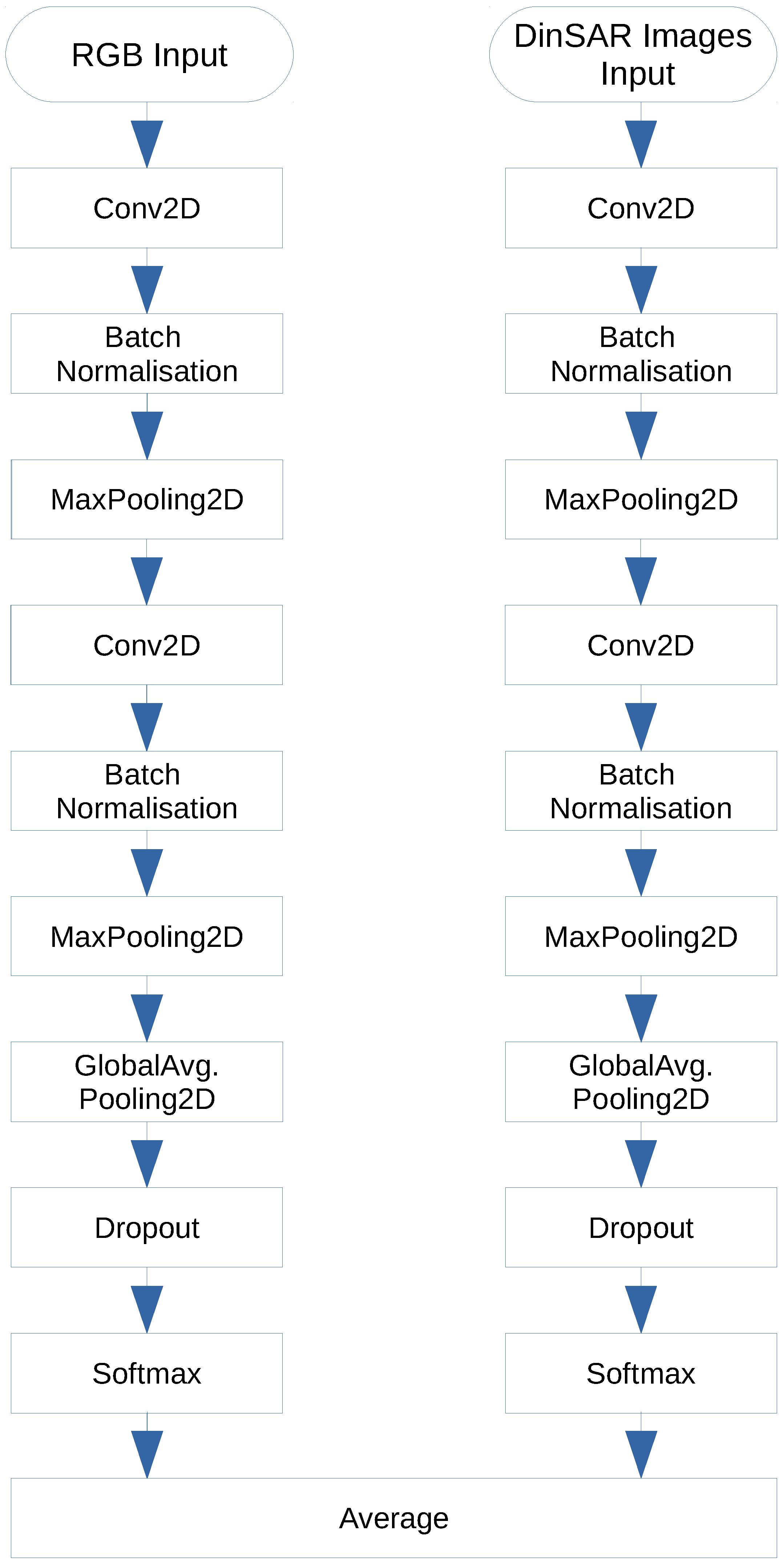
Figure 1. Architecture of ConvNet2, a 2-layer CNN [4].
Remotesensing 13 04394 g001
Figure 2. General form of the architecture of the FeatSpaceEnsNet family of transfer learning by feature extraction neural networks.
Remotesensing 13 04394 g002
Figure 3. General form of the architecture of the AvgEnsNet family of transfer learning by feature extraction neural networks.
Remotesensing 13 04394 g003
Figure 4. Local Binary Pattern of a positive blob in the dataset.
Remotesensing 13 04394 g004
Figure 5. Histogram of Oriented Gradients of a positive blob in the dataset.
Remotesensing 13 04394 g005
Figure 6. Sentinel-2 images of a true-positive blob of a construction site in Germiston.
Remotesensing 13 04394 g006
Figure 7. Google Earth image of a Germiston construction site.
Remotesensing 13 04394 g007
Figure 8. True-positive blob of a construction site in Germiston.
Remotesensing 13 04394 g008
Figure 9. Sentinel-2 images of a true-positive blob at a Thornhill Estates construction site.
Remotesensing 13 04394 g009
Figure 10. Google Earth image of a Thornhill Estates construction site.
Remotesensing 13 04394 g010
Figure 11. True-positive blob of a construction site in Thornhill Estate.
Remotesensing 13 04394 g011
Figure 12. Sentinel-2 images of a true-positive blob at a tailings mine dump retreatment site.
Remotesensing 13 04394 g012
Figure 13. Google Earth image of at a tailings mine dump retreatment site.
Remotesensing 13 04394 g013
Figure 14. True-positive blob of a tailings mine dump retreatment site.
Remotesensing 13 04394 g014
Figure 15. Sentinel-2 images of a true-positive blob of a factory yard in Alberton.
Remotesensing 13 04394 g015
Figure 16. Google Earth image of a factory yard in Alberton.
Remotesensing 13 04394 g016
Figure 17. True-positive blob of a factory yard in Alberton.
Remotesensing 13 04394 g017
Figure 18. Sentinel-2 images of a false-positive blob of crops in Pretoria Rural.
Remotesensing 13 04394 g018
Figure 19. False-positive blob of crops in Pretoria Rural.
Remotesensing 13 04394 g019
Figure 20. A difficult false-positive blob of trees in Hyde Park.
Remotesensing 13 04394 g020
Figure 21. Visualization of four of the false-positive blobs incorrectly classified by the best classifier.
Remotesensing 13 04394 g021aRemotesensing 13 04394 g021b
Figure 22. Visualization of four of the false-negative blobs incorrectly classified by the best classifier.
Remotesensing 13 04394 g022aRemotesensing 13 04394 g022b
Figure 23. Model performance with reference to parameter size, zoomed in to show models with performances above 78%, FeatSpaceEnsNet, AvgEnsNet, and HybridEnsNet are abbreviated as FSE, AE, and HE, respectively.
Remotesensing 13 04394 g023
Figure 24. Model performance with reference to the number of models, zoomed in to show models with performances above 78%, FeatSpaceEnsNet, AvgEnsNet, and HybridEnsNet are abbreviated as FSE, AE, and HE, respectively.
Remotesensing 13 04394 g024
Figure 25. AvgEnsNet 7 confusion matrix.
Remotesensing 13 04394 g025
Figure 26. HybridEnsNet 3 confusion matrix.
Remotesensing 13 04394 g026
Figure 27. FeatSpaceEnsNet 2 confusion matrix.
Remotesensing 13 04394 g027
Table 1. Ensemble definitions.
EnsembleModels
FeatSpaceEnsNet 1ResNet50 + ResNeXt50
FeatSpaceEnsNet 2ResNet50 + ResNeXt50 + EfficientNetB4
FeatSpaceEnsNet 3ResNet50 + ResNet101
FeatSpaceEnsNet 4ResNet50 + ResNet101 + ResNeXt50
FeatSpaceEnsNet 5ResNet50 + ResNet101 + ResNet152
FeatSpaceEnsNet 6ResNet50 + ResNet101 + Inception-ResnetV2
FeatSpaceEnsNet 7ResNet50 + Inception-ResnetV2
AvgEnsNet 1ResNet50 + Inception-ResnetV2
AvgEnsNet 2ResNet50 + ResNet101
AvgEnsNet 3ResNet50 + ResNeXt50
AvgEnsNet 4ResNet50 + ResNet101 + ResNeXt50
AvgEnsNet 5ResNet50 + ResNet101 + Inception-ResnetV2
AvgEnsNet 6ResNet50 + ResNet101 + ResNet152
AvgEnsNet 7ResNet50 + ResNeXt50 + EfficientNetB4
HybridEnsNet 1FeatSpaceEnsNet 3 + AvgEnsNet 2
HybridEnsNet 2FeatSpaceEnsNet 3 + AvgEnsNet 2 + IncResNetV2 + EffNetB0
HybridEnsNet 3FeatSpaceEnsNet 3 + AvgEnsNet 4 + IncResNetV2 + EffNetB0 + EffNetB4
HybridEnsNet 4FeatSpaceEnsNet 3 + AvgEnsNet 4 + IncResNetV2 + EffNetB0 + EffNetB4
+ ResNet152 + EffNetB7
HybridEnsNet 5FeatSpaceEnsNet 3 + AvgEnsNet 4 + IncResNetV2 + EffNetB0 + EffNetB4
+ ResNet152 + EffNetB7 + ResNet50V2 + ResNet152V2
Table 2. Performance of the deep learning and transfer learning single models applied with the corresponding number of parameters.
ModelMethodAcc. μ [%]Acc. σ 2 F1 ScorePrecisionRecall# Params
ResNet50TLFE83.7511.5030.8380.8380.83826 m
ResNet101TLFE83.4031.3410.8340.8340.83444 m
Inception-ResNetV2TLFE83.0901.2710.8310.8310.83156 m
EfficientNet B0TLFE82.2210.8460.8240.8250.8245 m
ResNeXt50TLFE81.4411.2850.8140.8150.81525 m
EfficientNet B4TLFE81.0411.3100.8110.8120.81119 m
ResNet50DLRI80.8515.1610.8080.8100.80926 m
ResNet152TLFE80.6772.3550.8070.8070.80760 m
EfficientNet B7TLFE79.6882.9540.7960.7960.79666 m
ResNet152V2TLFE78.8031.4030.7880.7900.78860 m
ResNet50V2TLFE78.8021.5790.7860.7910.78926 m
ResNet50TLFT71.07830.2880.7020.7320.71026 m
EfficientNet B4TLFT67.88124.4560.6620.7190.67919 m
EfficientNet B4DLRI65.60841.3380.6140.7530.65619 m
Table 3. Performance of the feature space ensemble models applied with the corresponding number of parameters.
ModelAcc. μ [%]Acc. σ 2 F1 ScorePrecisionRecall# Params
FeatSpaceEnsNet 284.8621.1080.8490.8500.84970 m
FeatSpaceEnsNet 384.6721.3500.8460.8470.84670 m
FeatSpaceEnsNet 484.5850.5010.8450.8450.84595 m
FeatSpaceEnsNet 784.4100.8480.8440.8440.84482 m
FeatSpaceEnsNet 684.2550.8020.8420.8420.842126 m
FeatSpaceEnsNet 184.0470.9080.8400.8400.84051 m
ResNet5083.7511.5030.8380.8380.83826 m
FeatSpaceEnsNet 583.5950.8110.8360.8360.836130 m
Table 4. Performance of the average ensemble models applied with the corresponding number of parameters.
ModelAcc. μ [%]Acc. σ 2 F1 ScorePrecisionRecall# Params
AvgEnsNet 784.8621.3740.8500.8500.85070 m
AvgEnsNet 484.7231.6900.8460.8470.84695 m
AvgEnsNet 584.3241.8720.8420.8430.842126 m
AvgEnsNet 184.0631.7390.8410.8420.84182 m
AvgEnsNet 283.9941.4210.8390.8390.83970 m
ResNet5083.7511.5030.8380.8380.83826 m
AvgEnsNet 383.7511.6670.8380.8390.83851 m
AvgEnsNet 683.4721.2240.8360.8360.836130 m
Table 5. Performance of the hybrid ensemble models applied with corresponding number of parameters.
ModelAcc. μ [%]Acc. σ 2 F1 ScorePrecisionRecall# Params
HybridEnsNet 384.7751.4640.8480.8490.848245 m
HybridEnsNet 284.7060.7940.8470.8470.847201 m
HybridEnsNet 484.4970.8290.8450.8450.845371 m
HybridEnsNet 184.2721.2190.8430.8430.843140 m
HybridEnsNet 584.1151.2540.8410.8420.842457 m
ResNet5083.7511.5030.8380.8380.83826 m
Table 6. Performance of all models and methods applied with the corresponding number of parameters.
ModelMethodAcc. μ [%]Acc. σ 2 F1 ScorePrecisionRecall
AvgEnsNet 7TLFE84.8621.3740.8500.8500.850
FeatSpaceEnsNet 2TLFE84.8621.1080.8490.8500.849
HybridEnsNet 3TLFE84.7751.4640.8480.8490.848
ResNet50TLFE83.7511.5030.8380.8380.838
ConvNet2ML82.6401.7000.8280.8310.828
LBP + RBF-SVMML70.5224.6190.7050.7070.705
LBP + RFML69.8962.8850.6990.7010.699
LBP + SVMML67.7600.8910.6780.6780.678
LBP + MLPML66.7544.7580.6660.6710.667
(HOG, LBP) + SVMML62.6396.2510.6260.6270.627
HOG + SVMML62.2575.8540.6230.6240.623
(HOG, LBP) + RFML62.2415.7680.6210.6250.623
(HOG, LBP) + MLPML61.9288.1430.6150.6220.619
HOG + MLPML61.5637.7160.6110.6220.614
HOG + RFML61.0074.4040.6080.6110.609
HOG + RBF-SVMML50.0000.0000.3300.2500.500
(HOG, LBP) + RBF-SVMML50.0000.0000.3300.2500.500
Table 7. Performance of best performing models under different cross-validation folds.
ModelMethodFoldsAcc. μ [%]Acc. σ 2 F1 ScorePrecisionRecall
AvgEnsNet 7TLFE 84.8621.3740.8500.8500.850
FeatSpaceEnsNet 2TLFE1084.8621.1080.8490.8500.850
ResNet50TLFE 83.7511.5030.8380.8380.838
LBP + RBF-SVMML 70.5224.6190.7050.7070.705
LBP + RFML 69.8962.8850.6990.7010.699
LBP + SVMML 67.7600.8910.6780.6780.678
AvgEnsNet 7TLFE585.1391.0120.8510.8520.851
FeatSpaceEnsNet 2TLFE 84.9321.0490.8490.8490.849
ResNet50TLFE 83.5071.7740.8350.8350.835
LBP + RFML 69.5143.5060.6940.6950.694
LBP + RBF-SVMML 69.2375.9010.6930.6940.693
LBP + SVMML 67.6401.1220.6780.6780.678
AvgEnsNet 7TLFE285.3300.4270.8530.8550.853
FeatSpaceEnsNet 2TLFE 85.2451.4110.8530.8530.853
ResNet50TLFE 83.4232.7640.8350.8350.835
LBP + RFML 70.8337.7980.7080.7080.708
LBP + RBF-SVMML 70.2286.1470.7030.7050.703
LBP + SVMML 68.2280.3620.6800.6830.680
Publisher’s Note: MDPI stays neutral with regard to jurisdictional claims in published maps and institutional affiliations.