
Mapping Aquifer Storage Properties Using S-Wave Velocity and InSAR-Derived Surface Displacement in the Kumamoto Area, Southwest Japan

 ,
, 
Abstract
:1. Introduction
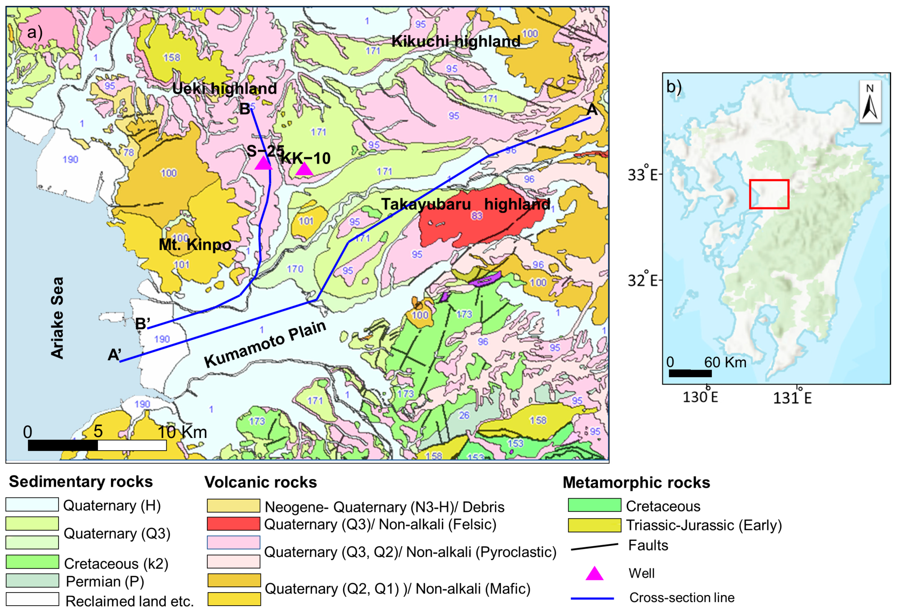
2. Study Area
3. Data Sets
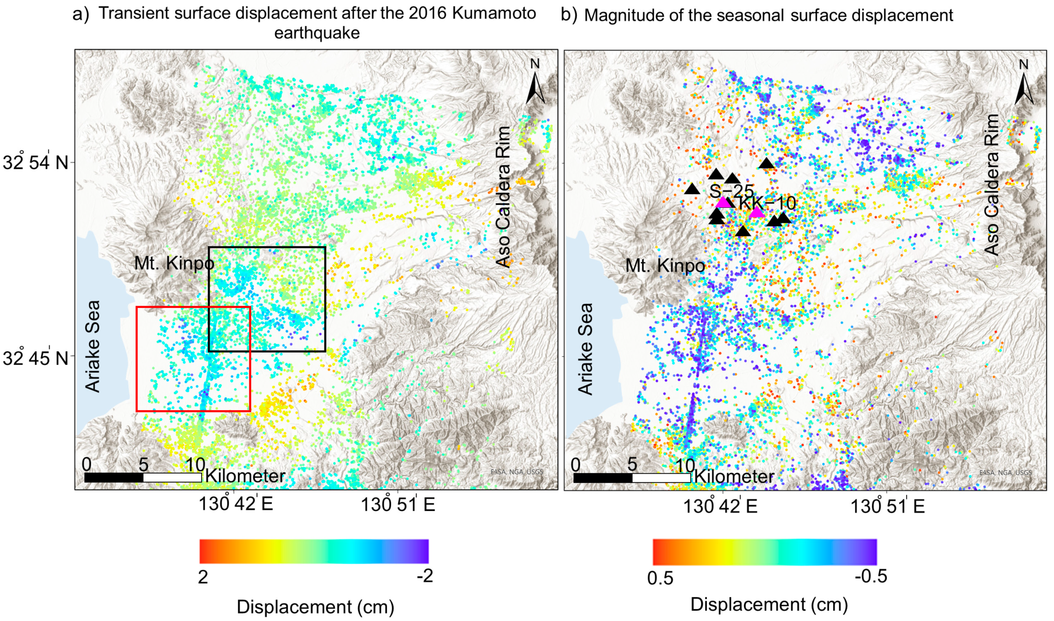
3.1. InSAR Data
3.2. Piezometric Data
3.3. Three-Dimensional S-Wave Velocity Model
- Estimation of a semivariogram model from the original data;
- Prediction of data at each of the observed points from the semivariogram;
- Estimation of a new semivariogram model and its weight from the predicted data;
- Repeating steps 2 and 3 creates a spectrum of the semivariogram models;
- Prediction of Vs and their standard errors at unmeasured locations using these weights.
4. Methodology: Mapping the Skeletal Storage Coefficient
5. Results and Interpretation
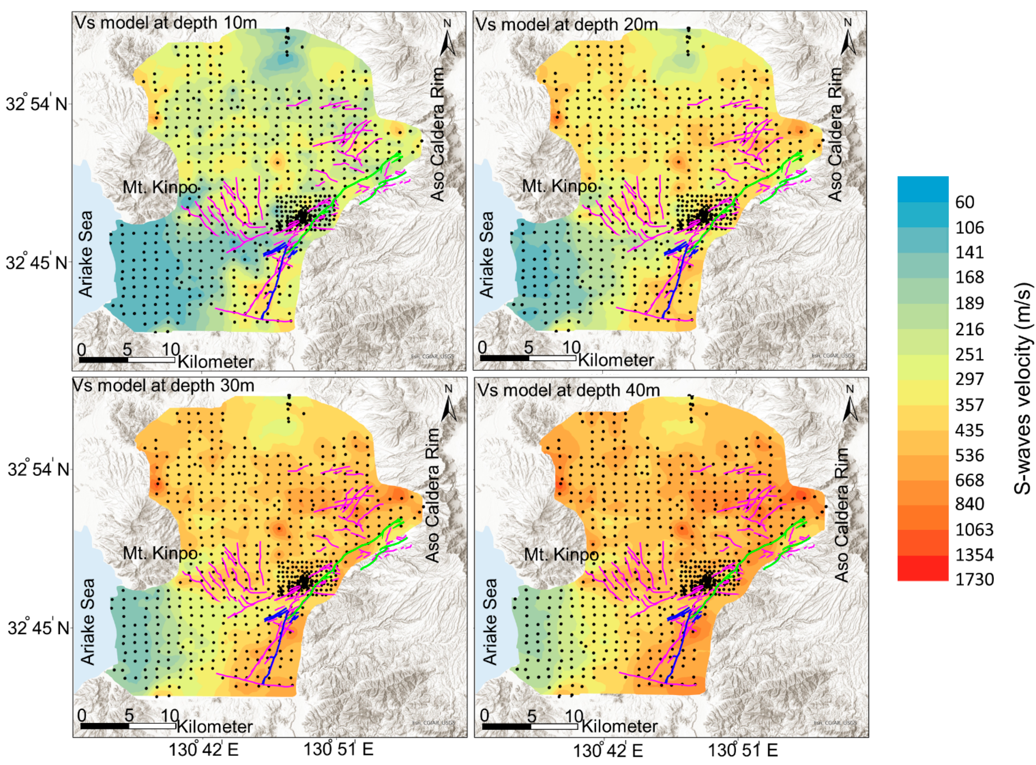
5.1. Three-Dimensional S-Wave Velocity

5.2. Skeletal Storage Coefficient and S-Waves Velocity Relationship
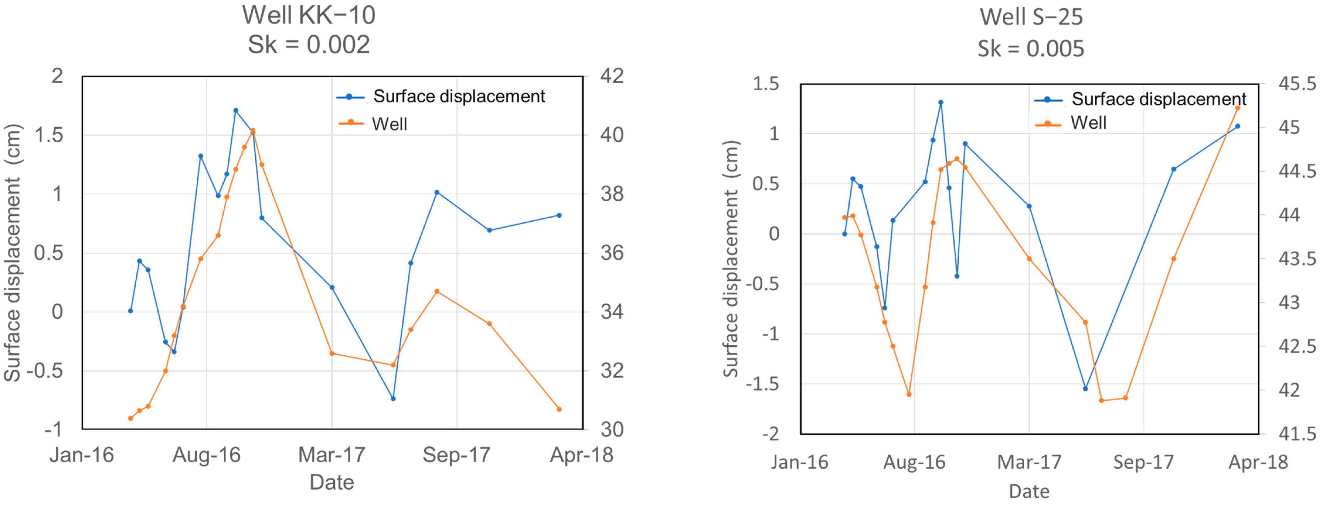
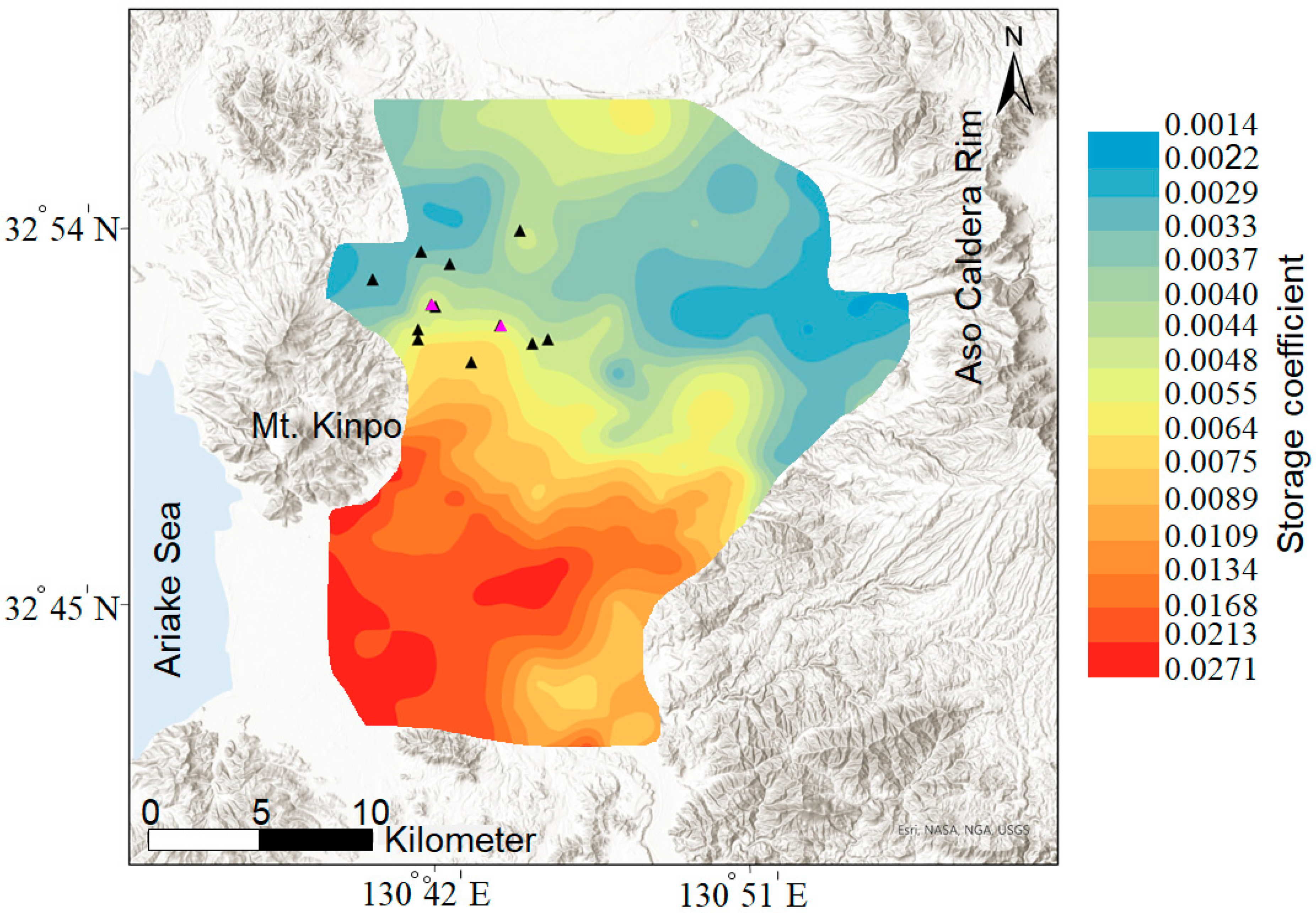
5.3. Mapping of the Skeletal Storage Coefficient to Monitor Groundwater Level from InSAR Data
6. Discussion
- (1)
- (2)
- Monitoring wells observe water from one aquifer in the saturated confined aquifer system [81]. Hoffmann et al. [23] mentioned that the estimated Sk would be inaccurate if hydraulic heads at piezometers do not represent the average local condition in the groundwater system. Most of the wells in this study correspond to a single confined aquifer based on the strainer depth information. Although there is a possibility that the temporal variation of the deeper aquifer may generate errors in estimating Sk, we assume the influence of the shallowest confined aquifer is dominant.
- (3)
- Error in measurements of InSAR displacement is due to atmospheric phase effects. In this study, temporal filtering was used to mitigate the error of atmospheric contribution. Because PSI displacements were consistent with the F3 solution of GEONET, GSI, Japan, the error in measurements of InSAR displacement could be minor.
- (4)
- Incomplete removal of the long-term subsidence from the land deformation time series for case studies of high subsidence rate. To completely separate long-term trends of subsidence and hydraulic head from their time series, daily or weekly measurements of InSAR and head time series for several years are required [82].
7. Conclusions
- The zone of low Vs found by the microtremor survey could have coincided with the Futagawa fault zone;
- Sk of the confined aquifer ranges between ~0.03 and 2 × 10⁻³, with an average of 7.23 × 10⁻³, reflecting semi-confined and confined conditions;
- An empirical relationship between the Sk and Vs was found, indicating that aquifer compressibility is linked to its stiffness and Vs;
- The map of Sk estimated from the empirical relationship correlates with the hydrogeological setting and can be used to estimate the spatiotemporal variation of groundwater-level based on the geodetic data.
Author Contributions
Funding
Institutional Review Board Statement
Informed Consent Statement
Data Availability Statement
Acknowledgments
Conflicts of Interest
References
- Banton, O.; Bangoy, L.M. A new method to determine storage coefficient from pumping test recovery data. Groundwater 1996, 34, 772–777. [Google Scholar] [CrossRef]
- Bardsley, W.E. DISCUSSION OF “Estimation of Storativity from Recovery Data,” by PN Ballukraya and KK Sharma. Groundwater 1992, 30, 272–273. [Google Scholar] [CrossRef]
- Chapuis, R.P. DISCUSSION OF “Estimation of Storativity from Recovery Data”, by PN Ballukraya and KK Sharma. Groundwater 1992, 30, 269–272. [Google Scholar] [CrossRef]
- Theis, C.V. The relation between the lowering of the piezometric surface and the rate and duration of discharge of a well using ground-water storage. Eos Trans. Am. Geophys. Union 1935, 16, 519–524. [Google Scholar] [CrossRef]
- Ballukraya, P.N.; Sharma, K.K. Estimation of storativity from recovery data. Groundwater 1991, 29, 495–498. [Google Scholar] [CrossRef]
- Jacob, C.E. The recovery method for determining the coefficient of transmissivity. US Geol. Surv. Water Supply Pap. 1963, 1536–I, 281–292. [Google Scholar]
- Shah, T.; Molden, D.; Sakthivadivel, R.; Seckler, D. Global groundwater situation: Opportunities and challenges. Econ. Polit. Wkly. 2001, 4142–4150. [Google Scholar]
- Gabrysch, R.K.; Bonnet, C.W. Land-Surface Subsidence in the Houston-Galveston Region, Texas; Texas Water Development Board: Austin, TX, USA, 1975; Volume 74. [Google Scholar]
- Hix, G.L. Land subsidence and ground water withdrawal. Water Well J. 1995, 49, 37–39. [Google Scholar]
- Sun, H.; Grandstaff, D.; Shagam, R. Land subsidence due to groundwater withdrawal: Potential damage of subsidence and sea level rise in southern New Jersey, USA. Environ. Geol. 1999, 37, 290–296. [Google Scholar] [CrossRef]
- Zhang, Y.; Xue, Y.-Q.; Wu, J.-C.; Yu, J.; Wei, Z.-X.; Li, Q.-F. Land subsidence and earth fissures due to groundwater withdrawal in the Southern Yangtse Delta, China. Environ. Geol. 2008, 55, 751. [Google Scholar] [CrossRef]
- Modoni, G.; Darini, G.; Spacagna, R.L.; Saroli, M.; Russo, G.; Croce, P. Spatial analysis of land subsidence induced by groundwater withdrawal. Eng. Geol. 2013, 167, 59–71. [Google Scholar] [CrossRef]
- Khakim, M.Y.N.; Tsuji, T.; Matsuoka, T. Lithology-controlled subsidence and seasonal aquifer response in the Bandung basin, Indonesia, observed by synthetic aperture radar interferometry. Int. J. Appl. Earth Obs. Geoinf. 2014, 32, 199–207. [Google Scholar] [CrossRef] [Green Version]
- Ishitsuka, K.; Fukushima, Y.; Tsuji, T.; Yamada, Y.; Matsuoka, T.; Giao, P.H. Natural surface rebound of the Bangkok plain and aquifer characterization by persistent scatterer interferometry. Geochem. Geophys. Geosystems. 2014, 15, 965–974. [Google Scholar] [CrossRef]
- Zhu, L.; Gong, H.; Li, X.; Wang, R.; Chen, B.; Dai, Z.; Teatini, P. Land subsidence due to groundwater withdrawal in the northern Beijing plain, China. Eng. Geol. 2015, 193, 243–255. [Google Scholar] [CrossRef]
- Terzaghi, K. Erdbaumechanik auf Bodenphysikalischer Grundlage; Deuticke, F., Leipzig, Eds.; Food and Agriculture Organization of the United Nations: Beltsville, MD, USA; Washington, DC, USA, 1925. [Google Scholar]
- Chen, J.; Knight, R.; Zebker, H.A.; Schreüder, W.A. Confined aquifer head measurements and storage properties in the San Luis Valley, Colorado, from spaceborne InSAR observations. Water Resour. Res. 2016, 52, 3623–3636. [Google Scholar] [CrossRef] [Green Version]
- Riley, F.S. Analysis of borehole extensometer data from central California. Land Subsid. 1969, 2, 423–431. [Google Scholar]
- Chaussard, E.; Bürgmann, R.; Shirzaei, M.; Fielding, E.J.; Baker, B. Predictability of hydraulic head changes and characterization of aquifer-system and fault properties from InSAR-derived ground deformation. J. Geophys. Res. Solid Earth 2014, 119, 6572–6590. [Google Scholar] [CrossRef]
- Ezquerro, P.; Herrera, G.; Marchamalo, M.; Tomás, R.; Béjar-Pizarro, M.; Martínez, R. A quasi-elastic aquifer deformational behavior: Madrid aquifer case study. J. Hydrol. 2014, 519, 1192–1204. [Google Scholar] [CrossRef] [Green Version]
- Reeves, J.A.; Knight, R.; Zebker, H.A.; Kitanidis, P.K.; Schreüder, W.A. Estimating temporal changes in hydraulic head using InSAR data in the San Luis Valley, Colorado. Water Resour. Res. 2014, 50, 4459–4473. [Google Scholar] [CrossRef]
- Béjar-Pizarro, M.; Ezquerro, P.; Herrera, G.; Tomás, R.; Guardiola-Albert, C.; Hernández, J.M.R.; Merodo, J.A.F.; Marchamalo, M.; Martínez, R. Mapping groundwater level and aquifer storage variations from InSAR measurements in the Madrid aquifer, Central Spain. J. Hydrol. 2017, 547, 678–689. [Google Scholar] [CrossRef] [Green Version]
- Hoffmann, J.; Zebker, H.A.; Galloway, D.L.; Amelung, F. Seasonal subsidence and rebound in Las Vegas Valley, Nevada, observed by synthetic aperture radar interferometry. Water Resour. Res. 2001, 37, 1551–1566. [Google Scholar] [CrossRef]
- Foti, S.; Hollender, F.; Garofalo, F.; Albarello, D.; Asten, M.; Bard, P.-Y.; Comina, C.; Cornou, C.; Cox, B.; Di Giulio, G.; et al. Guidelines for the good practice of surface wave analysis: A product of the InterPACIFIC project. Bull. Earthq. Eng. 2018, 16, 2367–2420. [Google Scholar] [CrossRef]
- Okada, H.; Suto, K. The Microtremor Survey Method; Society of Exploration Geophysicists: Houston, TX, USA, 2003; ISBN 1560801204. [Google Scholar]
- Khalili, M.; Mirzakurdeh, A.V. Fault detection using microtremor data (HVSR-based approach) and electrical resistivity survey. J. Rock Mech. Geotech. Eng. 2019, 11, 400–408. [Google Scholar] [CrossRef]
- Wu, C.F.; Huang, H.C. Detection of a fracture zone using microtremor array measurementDetection of a fracture zone. Geophysics 2019, 84, 33–40. [Google Scholar] [CrossRef]
- Du, Y.N.; Xu, P.F.; Ling, S.Q. Microtremor survey of soil-rock mixture landslide: A case study of landslide in Baidian Township, Hengyang City. Chinese J. Geophys. 2018, 61, 1596–1604. [Google Scholar]
- Bonnefoy-Claudet, S.; Baize, S.; Bonilla, L.F.; Berge-Thierry, C.; Pasten, C.; Campos, J.; Verdugo, R. Site effect evaluation in the basin of Santiago de Chile using ambient noise measurements. Geophys. J. Int. 2009, 176, 925–937. [Google Scholar] [CrossRef] [Green Version]
- Xu, P.; Ling, S.; Zhang, D.; Dai, K.; Li, C.; Du, J. Mapping deeply-buried geothermal faults using microtremor array analysis. Geophys. J. Int. 2012, 188, 115–122. [Google Scholar] [CrossRef]
- Xu, P.; Li, S.H.; Du, J.G.; Ling, S.Q.; Guo, H.L. Microtremor Survey Method: A New Geophysical Method for Dividing Strata and Detecting the Buried Fault Structures; Acta Petrologica Sinica: Beijing, China, 2013; Volume 29, pp. 1841–1845. [Google Scholar]
- Tian, B.; Xu, P.; Ling, S.; Du, J.; Xu, X.; Pang, Z. Application effectiveness of the microtremor survey method in the exploration of geothermal resources. J. Geophys. Eng. 2017, 14, 1283–1289. [Google Scholar] [CrossRef] [Green Version]
- Rezaei, S.; Choobbasti, A.J. Liquefaction assessment using microtremor measurement, conventional method and artificial neural network case study: Babol, Iran. Front. Struct. Civ. Eng. 2014, 8, 292–307. [Google Scholar] [CrossRef]
- Takahashi, K.; Tsuji, T.; Ikeda, T.; Nimiya, H.; Nagata, Y.; Suemoto, Y. Underground structures associated with horizontal sliding at Uchinomaki hot springs, Kyushu, Japan, during the 2016 Kumamoto earthquake. Earth Planets Sp. 2019, 71, 87. [Google Scholar] [CrossRef]
- Castagna, J.P.; Batzle, M.L.; Eastwood, R.L. Relationships between compressional-wave and shear-wave velocities in clastic silicate rocks. Geophysics 1985, 50, 571–581. [Google Scholar] [CrossRef]
- Grelle, G.; Guadagno, F.M. Seismic refraction methodology for groundwater level determination:“Water seismic index. ” J. Appl. Geophys. 2009, 68, 301–320. [Google Scholar] [CrossRef]
- Serdyukov, A.S.; Yablokov, A.V.; Chernyshov, G.S.; Azarov, A.V. The surface waves-based seismic exploration of soil and ground water. In IOP Conference Series: Earth and Environmental Science; IOP Publishing: Bristol, England, 2017; Volume 53, p. 12010. [Google Scholar]
- Cha, M.; Santamarina, J.C.; Kim, H.-S.; Cho, G.-C. Small-strain stiffness, shear-wave velocity, and soil compressibility. J. Geotech. Geoenviron. Eng. 2014, 140, 6014011. [Google Scholar] [CrossRef] [Green Version]
- Martin, C.D.; Davison, C.C.; Kozak, E.T. Characterizing normal stiffness and hydraulic conductivity of a major shear zone in granite. In Proceedings of the International Symposium on Rock Joints, Loen, France, 4–6 June 1990; pp. 549–556. [Google Scholar]
- Rutqvist, J.; Noorishad, J.; Tsang, C.; Stephansson, O. Determination of fracture storativity in hard rocks using high-pressure injection testing. Water Resour. Res. 1998, 34, 2551–2560. [Google Scholar] [CrossRef]
- Ishitsuka, K.; Tsuji, T.; Matsuoka, T. Surface Displacement Around the Ezu Lake and the Suizenji Area Associated with the 2016 Kumamoto Earthquake. J. Remote Sens. Soc. Jpn. 2016, 36, 218–222. [Google Scholar]
- Ishitsuka, K.; Tsuji, T.; Lin, W.; Kagabu, M.; Shimada, J. Seasonal and transient surface displacements in the Kumamoto area, Japan, associated with the 2016 Kumamoto earthquake: Implications for seismic-induced groundwater level change. Earth Planets Sp. 2020, 72, 144. [Google Scholar] [CrossRef]
- Hossain, S. Geochemical modeling of groundwater evolution in a volcanic aquifer system of Kumamoto area, Japan. In American Geophysical Union (AGU) Fall Meeting Abstracts; American Geophysical Union: Washington, DC, USA, 2013. [Google Scholar]
- Hossain, S. Geochemical processes controlling fluoride enrichment in groundwater at the western part of Kumamoto area, Japan. Water Air Soil Pollut. 2016, 227, 385. [Google Scholar] [CrossRef]
- Hosono, T.; Hossain, S.; Shimada, J. Hydrobiogeochemical evolution along the regional groundwater flow systems in volcanic aquifers in Kumamoto, Japan. Environ. Earth Sci. 2020, 79, 410. [Google Scholar] [CrossRef]
- Mahara, Y.; Igarashi, T.; Kudo, A. Groundwater Origin and Evolution from Dissolved Helium Isotopes in the Kumamoto Plain. 1997. Available online: https://www.osti.gov/etdeweb/biblio/307537 (accessed on 1 September 2021).
- Fujiwara, S.; Yarai, H.; Kobayashi, T.; Morishita, Y.; Nakano, T.; Miyahara, B.; Nakai, H.; Miura, Y.; Ueshiba, H.; Kakiage, Y.; et al. Small-displacement linear surface ruptures of the 2016 Kumamoto earthquake sequence detected by ALOS-2 SAR interferometry. Earth Planets Sp. 2016, 68, 160. [Google Scholar] [CrossRef] [Green Version]
- Goto, H. Geomorphic features of surface ruptures associated with the 2016 Kumamoto earthquake in and around the downtown of Kumamoto City, and implications on triggered slip along active faults. Earth Planets Sp. 2017, 69, 26. [Google Scholar] [CrossRef] [Green Version]
- Ishitsuka, K.; Tsuji, T. Mapping Surface Displacements and Aquifer Characteristics Around the Kumamoto Plain, Japan, Using Persistent Scatterer Interferometry. In Proceedings of the IGARSS 2019-2019 IEEE International Geoscience and Remote Sensing Symposium, Yokohama, Japan, 28 July–2 August 2019. [Google Scholar]
- Tsuji, T.; Ishibashi, J.; Ishitsuka, K.; Kamata, R. Horizontal sliding of kilometre-scale hot spring area during the 2016 Kumamoto earthquake. Sci. Rep. 2017, 7, 42947. [Google Scholar] [CrossRef] [PubMed] [Green Version]
- Taniguchi, M.; Burnett, K.M.; Shimada, J.; Hosono, T.; Wada, C.A.; Ide, K. Recovery of lost nexus synergy via payment for environmental services in Kumamoto, Japan. Front. Environ. Sci. 2019, 7, 28. [Google Scholar] [CrossRef] [Green Version]
- Hosono, T.; Tokunaga, T.; Kagabu, M.; Nakata, H.; Orishikida, T.; Lin, I.-T.; Shimada, J. The use of δ15N and δ18O tracers with an understanding of groundwater flow dynamics for evaluating the origins and attenuation mechanisms of nitrate pollution. Water Res. 2013, 47, 2661–2675. [Google Scholar] [CrossRef] [PubMed]
- Parvin, M.; Tadakuma, N.; Asaue, H.; Koike, K. Delineation and interpretation of spatial coseismic response of groundwater levels in shallow and deep parts of an alluvial plain to different earthquakes: A case study of the Kumamoto City area, southwest Japan. J. Asian Earth Sci. 2014, 83, 35–47. [Google Scholar] [CrossRef]
- Nakagawa, K.; Yu, Z.-Q.; Berndtsson, R.; Hosono, T. Temporal characteristics of groundwater chemistry affected by the 2016 Kumamoto earthquake using self-organizing maps. J. Hydrol. 2020, 582, 124519. [Google Scholar] [CrossRef]
- Geological Map of Japan 1:1000000, 3rd ed.; 2nd [CD-ROM] version; National Institute of Advanced Industrial Science and Technology (AIST)—Geological Survey of Japan (GSJ): Ikeda, Osaka, Japan, 2003. (In Japanese)
- Ferretti, A.; Prati, C.; Rocca, F. Permanent scatterers in SAR interferometry. IEEE Trans. Geosci. Remote Sens. 2001, 39, 8–20. [Google Scholar] [CrossRef]
- Kampes, B.M. Radar Interferometry; Springer: Dordrechter, The Netherlands, 2006; Volume 12. [Google Scholar]
- Costantini, M.; Rosen, P.A. A generalized phase unwrapping approach for sparse data. In Proceedings of the IEEE 1999 International Geoscience and Remote Sensing Symposium. IGARSS’99 (Cat. No. 99CH36293), Hamburg, Germany, 28 June–2 July 1999; Volume 1, pp. 267–269. [Google Scholar]
- Cho, I.; Senna, S.; Fujiwara, H. Miniature array analysis of microtremors. Geophysics 2013, 78, 13–23. [Google Scholar] [CrossRef]
- Senna, S.; Wakai, A.; Suzuki, H.; Yatagai, A.; Matsuyama, H.; Fujiwara, H. Modeling of the subsurface structure from the seismic bedrock to the ground surface for a broadband strong motion evaluation in Kumamoto plain. J. Disaster Res. 2018, 13, 917–927. [Google Scholar] [CrossRef]
- Cho, I.; Senna, S. Constructing a system to explore shallow velocity structures using a miniature microtremor array. Synth. Engl. Ed. 2016, 9, 87–98. [Google Scholar]
- Arai, H.; Tokimatsu, K. S-wave velocity profiling by inversion of microtremor H/V spectrum. Bull. Seismol. Soc. Am. 2004, 94, 53–63. [Google Scholar] [CrossRef]
- Pelekis, P.C.; Athanasopoulos, G.A. An overview of surface wave methods and a reliability study of a simplified inversion technique. Soil Dyn. Earthq. Eng. 2011, 31, 1654–1668. [Google Scholar] [CrossRef]
- Krivoruchko, K. Empirical bayesian kriging. ArcUser Fall 2012, 15, 6–10. [Google Scholar]
- Todd, D.K.; Mays, L.W. Groundwater Hydrology; John Willey & Sons. Inc.: New York, NY, USA, 1980; Volume 535. [Google Scholar]
- Galloway, D.L.; Burbey, T.J. Regional land subsidence accompanying groundwater extraction. Hydrogeol. J. 2011, 19, 1459–1486. [Google Scholar] [CrossRef]
- Reeves, J.A. Using Interferometric Synthetic Aperture Radar Data to Improve Estimates of Hydraulic Head in the San Luis Valley, Colorado; Stanford University: Stanford, CA, USA, 2013; ISBN 9798678101488. [Google Scholar]
- Venkatramaiah, C. Geotechnical Engineering; New Age International: New Delhi, India, 1995; ISBN 812240829X. [Google Scholar]
- Li, C.; Chen, X.; Du, Z. A new relationship of rock compressibility with porosity. In Proceedings of the SPE Asia Pacific Oil and Gas Conference and Exhibition, Perth, Australia, 18–20 October 2004. [Google Scholar]
- Aysen, A. Soil Mechanics: Basic Concepts and Engineering Applications; CRC Press: Boca Raton, FL, USA, 2002; ISBN 9058093581. [Google Scholar]
- Duffy, B.G. Development of Multichannel Analysis of Surface Waves (MASW) for Characterising the Internal Structure of Active Fault Zones as A Predictive Method of Identifying the Distribution of Ground Deformation. Master’s Thesis, University of Canterbury, Christchurch, New Zealand, 2008. [Google Scholar]
- National Research Council Liquefaction of Soils during Earthquakes; National Academy Press: Washington, DC, USA, 1985; p. 240.
- Pitilakis, K.D. Earthquake Geotechnical Engineering: 4th International Conference on Earthquake Geotechnical Engineering-Invited Lectures; Springer Science & Business Media: Berlin, Germany, 2007; Volume 6, ISBN 1402058934. [Google Scholar]
- Agency, F.E.M. NEHRP Recommended Provisions for Seismic Regulations for New Buildings and Other Structures; Federal Emergency Management Agency (FEMA): Washington, DC, USA, 2003. [Google Scholar]
- Committee, A. Minimum Design Loads for Buildings and Other Structures (ASCE/SEI 7-10); American Society of Civil Engineers: Reston, VA, USA, 2010. [Google Scholar]
- Duffy, B.; Campbell, J.; Finnemore, M.; Gomez, C. Defining fault avoidance zones and associated geotechnical properties using MASW: A case study on the Springfield Fault, New Zealand. Eng. Geol. 2014, 183, 216–229. [Google Scholar] [CrossRef] [Green Version]
- Nakata, T.; Imaizumi, T. Digital Active Fault Map of Japan; University of Tokyo Press: Tokyo, Japan, 2002. [Google Scholar]
- Lohman, S.W. Ground-Water Hydraulics; US Government Printing Office: Washington, DC, USA, 1972; Volume 708. [Google Scholar]
- Rasmussen, W.C. Permeability and Storage of Heterogeneous Aquifers in the United States; International Union of Geodesy and Geophysics: Berkeley, August, 1963. [Google Scholar]
- Wilson, S.; Wöhling, T. Wairau River-Wairau Aquifer Interaction. Envirolink Report 1003-5-R1, 49p. 2015. Available online: https://www.marlborough.govt.nz/repository/libraries/id:1w1mps0ir17q9sgxanf9/hierarchy/Documents/Environment/Groundwater/Wairau%20Aquifer%20Project%20Reports%20List/WairauRiverAquiferInteraction.pdf (accessed on 1 September 2021).
- Burbey, T.J. Effects of horizontal strain in estimating specific storage and compaction in confined and leaky aquifer systems. Hydrogeol. J. 1999, 7, 521–532. [Google Scholar] [CrossRef]
- Rezaei, A.; Mousavi, Z. Characterization of land deformation, hydraulic head, and aquifer properties of the Gorgan confined aquifer, Iran, from InSAR observations. J. Hydrol. 2019, 579, 124196. [Google Scholar] [CrossRef]


| Well | Depth of Strainer (m) (Top, Bottom) | Vs (m/s) | Sk Estimated Using InSAR | Standard Error of Sk Estimated Using InSAR × 10−3 | p-Value | Correlation Coefficient |
|---|---|---|---|---|---|---|
| SS-004 | (52.0, 107.0) | 537 | 0.012 | 3.9 | 0.0569 | 0.5191 |
| SS-006 | (30.3, 88.5) | 263 | 0.011 | 4.8 | 0.0432 | 0.5108 |
| SS-003 | (64.0, 130.0) | 533 | 0.002 | 0.5 | 0.0075 | 0.6594 |
| SS-18 | (59.0, 89.0) | 432 | 0.003 | 0.1 | 0.0148 | 0.5794 |
| SS-005 | (3.5, 17.0) | 263 | 0.030 | 13.3 | 0.043 | 0.5469 |
| SS-17 | (100.5, 144.5) | 455 | 0.003 | 2.6 | 0.243 | 0.3843 |
| S-25 | (83.5, 94.5) | 288 | 0.005 | 2.0 | 0.0162 | 0.5866 |
| SS-16 | Unknown | 532 | 0.003 | 1.6 | 0.047 | 0.503 |
| SS-127 | (80.0, 146.0) | 295 | 0.007 | 5.8 | 0.027 | 0.5868 |
| SS-15 | (88.0, 170.0) | 455 | 0.004 | 1.6 | 0.0228 | 0.5823 |
| K-K7 | (51.5, 91.5) | 700 | 0.006 | 2.9 | 0.0197 | 0.4825 |
| KK-10 | (88.0, 98.0) | 439 | 0.002 | 0.4 | 0.0011 | 0.7073 |
| K-K3 | (43.0, 70.5) | 514 | 0.006 | 1.5 | 6.74 × 10−05 | 0.7112 |
Publisher’s Note: MDPI stays neutral with regard to jurisdictional claims in published maps and institutional affiliations. |
© 2021 by the authors. Licensee MDPI, Basel, Switzerland. This article is an open access article distributed under the terms and conditions of the Creative Commons Attribution (CC BY) license (https://creativecommons.org/licenses/by/4.0/).
Share and Cite
Mourad, M.; Tsuji, T.; Ikeda, T.; Ishitsuka, K.; Senna, S.; Ide, K. Mapping Aquifer Storage Properties Using S-Wave Velocity and InSAR-Derived Surface Displacement in the Kumamoto Area, Southwest Japan. Remote Sens. 2021, 13, 4391. https://doi.org/10.3390/rs13214391
Mourad M, Tsuji T, Ikeda T, Ishitsuka K, Senna S, Ide K. Mapping Aquifer Storage Properties Using S-Wave Velocity and InSAR-Derived Surface Displacement in the Kumamoto Area, Southwest Japan. Remote Sensing. 2021; 13(21):4391. https://doi.org/10.3390/rs13214391
Chicago/Turabian StyleMourad, Mohamed, Takeshi Tsuji, Tatsunori Ikeda, Kazuya Ishitsuka, Shigeki Senna, and Kiyoshi Ide. 2021. "Mapping Aquifer Storage Properties Using S-Wave Velocity and InSAR-Derived Surface Displacement in the Kumamoto Area, Southwest Japan" Remote Sensing 13, no. 21: 4391. https://doi.org/10.3390/rs13214391
APA StyleMourad, M., Tsuji, T., Ikeda, T., Ishitsuka, K., Senna, S., & Ide, K. (2021). Mapping Aquifer Storage Properties Using S-Wave Velocity and InSAR-Derived Surface Displacement in the Kumamoto Area, Southwest Japan. Remote Sensing, 13(21), 4391. https://doi.org/10.3390/rs13214391