Learned Hyperspectral Compression Using a Student’s T Hyperprior

Abstract

Hyperspectral compression is one of the most common techniques in hyperspectral image processing. Most recent learned image compression methods have exhibited excellent rate-distortion performance for natural images, but they have not been fully explored for hyperspectral compression tasks. In this paper, we propose a trainable network architecture for hyperspectral compression tasks, which not only considers the anisotropic characteristic of hyperspectral images but also embeds an accurate entropy model using the non-Gaussian prior knowledge of hyperspectral images and nonlinear transform. Specifically, we first design a spatial-spectral block, involving a spatial net and a spectral net as the base components of the core autoencoder, which is more consistent with the anisotropic hyperspectral cubes than the existing compression methods based on deep learning. Then, we design a Student’s T hyperprior that merges the statistics of the latents and the side information concepts into a unified neural network to provide an accurate entropy model used for entropy coding. This not only remarkably enhances the flexibility of the entropy model by adjusting various values of the degree of freedom, but also leads to a superior rate-distortion performance. The results illustrate that the proposed compression scheme supersedes the Gaussian hyperprior universally for virtually all learned natural image codecs and the optimal linear transform coding methods for hyperspectral compression. Specifically, the proposed method provides a 1.51% to 59.95% average increase in peak signal-to-noise ratio, a 0.17% to 18.17% average increase in the structural similarity index metric and a 6.15% to 64.60% average reduction in spectral angle mapping over three public hyperspectral datasets compared to the Gaussian hyperprior and the optimal linear transform coding methods.

1. Introduction

Different from the universal RGB images, hyperspectral images (HSIs) characterize each pixel of the observed materials with a unique spectral signature that is composed of dozens or even hundreds of components corresponding to different wavelengths [1]. This provides a much finer knowledge of the scenes, making HSIs advantageous and crucial tools for some computer vision tasks, such as object categorization [2,3], recognition [4] and restoration [5]. However, the benefits of the additional information also pose challenges for the HSI sensor storage capacity and the attainable transmission bandwidth. Therefore, an effective compression technology is vital for HSI processing tasks.

Ideally, the compressed HSIs should preserve all information without distortion. Due to the restricted storage capacity or transmission bandwidth, a compression technique with a high compression rate is a feasible solution to address the limitations of practical application. Since the compression ratios are usually approximately three or four in the current lossless HSI compression algorithms [6], lossy compression under an acceptable rate-distortion tradeoff is becoming an increasingly favorable choice.

As a classical lossy compression method, Transform Coding (TC) has been widely used for HSI compression with reasonable complexity. It first maps pixels from high-dimensional pixel space into a compact latent space by decorrelating transforms in order to exploit the spatial and spectral correlation and then quantizes and codes each latent separately [7]. According to the difference of decorrelating transform methods, the TC method contains linear and nonlinear transform algorithms.

Representative linear transform coding-based image compression techniques include the Joint Photographic Experts Group (JPEG) 2000 [8], removing high-frequency components from images with discrete wavelet transform, and set partitioning methods, providing a sequence for significant pixels with a tree or block splitting algorithm, such as set partitioning in hierarchical trees (SPIHT) [9] and embedded zero block coding (EZBC) [10]. Based on the requirement of HSI compression, two common strategies are proposed. First, the transforms in these methods are directly designed in 3D form to match the three-dimensional characteristic of HSIs, such as 3D discrete cosine transform (3D-DCT) [11] and 3D discrete wavelet transform (3D-DWT) [12]. However, not all methods benefit from direct 3D transform. For example, JP3D (part 10 in JPEG2000) [13] is designed for 3D image compression, yet does not work well for HSIs due to the fact that the 3D transform in JP3D is isotropic, but the spectral correlation in HSIs is much higher than the spatial direction [14]. Thus, since HSIs can be viewed as an anisotropic joint of 1D spectra and 2D space, a 1D transform (such as the Karhunen–Loève Transform (KLT), DCT or DWT) in the spectral dimension combined with a 2D transform in space has become a popular and effective solution [15,16,17,18].

However, these linear transforms often implicitly or explicitly assume that the data source satisfies joint Gaussian distribution. Although such an assumption allows for a simple closed-form solution, it may degrade the performance of subsequent entropy coding and rate allocation and thus lead to a suboptimal compression result. This is mainly attributed to the following two reasons. First, some researchers have proven that real-world HSIs represented with separable spatial-spectral bases have marginal distributions of individual coefficients that show greater kurtosis and have heavier tails than HSIs with the same variance of the Gaussian distribution [19]. At the same time, the joint distributions of different spatial coefficients show variance dependencies at the same location. Therefore, these results illustrate that the HSI source is non-Gaussian, and linear transforms are not the optimal compression methods for hyperspectral data. Second, the Gaussian assumption of the data source also makes the latent representation for HSIs a Gaussian distribution after a linear transform. This gives rise to deviation in the entropy modeling of the latent representation and finally causes a mismatch rate estimation. To address these problems, nonlinear transform coding combined with a non-Gaussian prior needs to be considered in HSI compression tasks because the nonlinearity possesses a more powerful representation capability than traditional linear transforms and a non-Gaussian prior may be helpful for accurate entropy modeling.

Fortunately, the artificial neural network (ANN) is a typical nonlinear transform framework that implements transforms by approximating nonlinear functions, with the ability of mapping pixels into a more compact space than traditional linear transforms; it has achieved excellent results in natural image compression [20,21,22,23,24,25,26,27,28,29,30,31,32,33,34]. Autoencoder [35] is one of the representative ANN frameworks implementing such nonlinear transform coding [22,36,37]. Moreover, the merger of variational Bayesian theory makes autoencoder-based compression methods more easily explained from the perspective of information quantity [38].

Furthermore, since the latent representation obtained from nonlinear transform is compressed with entropy coding methods via the entropy model, improving the capacity of the entropy model also needs to be considered. Earlier works usually use a fully factorized density [21] to construct entropy models to estimate the probability distribution of the latents. Advanced methods have improved the accuracy of the entropy model. The entropy model in [20] is implemented with a fixed or even complex model based on the context. To model the relationships over latents, a conditional probability model [39] is proposed, which resembles the recurrent networks idea in [40]. To reduce the time complexity, a hyperprior [30] linked to the concept of side information is employed, which enhances the accuracy of the entropy model by introducing small additional bits. Although the hyperprior-based method is flexible and has high efficiency in the image compression task, the rationality of the existing hyperprior still depends on the assumption that the statistics of each latent follow a Gaussian distribution, which may not be appropriate in many real cases. This is because the latent representation is of non-Gaussian behavior after nonlinear transform, regardless of whether the data source has a Gaussian or non-Gaussian distribution.

In view of the existing ANN-based image compression methods, establishing a nonlinear transform for HSIs becomes feasible. Because most of the ANN-based compression works focus on natural images (RGB) [41], we need to combine the characteristics of HSIs for an optimal compression result. First, the designing of the network architecture should be consistent with the anisotropic hyperspectral cubes. Moreover, proposing a rational hyperprior to learn an accurate entropy model over compressed HSIs for entropy coding is also another key factor for obtaining the optimal rate-distortion performance.

Based on the above analysis, this paper explores a specific end-to-end learning-based framework for the HSI compression task. The contributions of this research are as follows.

(1) A spatial and spectral network (SS-Net) is developed and embedded into the comprehensive ANN-based compression architecture so as to both realize the nonlinear transform and take into account the anisotropic characteristic of HSIs. The proposed architecture links cascades of convolutional neural networks to the anisotropic HSI cubes, which can possess a more powerful representation capability than traditional linear transform codecs.

(2) A Student’s T hyperprior that merges the statistics of the latents and the side information concept into a unified neural network is proposed to learn an accurate entropy model for entropy coding, which can not only increase the flexibility of entropy model, but also greatly improve the efficiency of entropy coding.

(3) The experimental results show that the proposed compression framework can outperform the commonly used linear transform coding methods for HSI compression in terms of rate-distortion performance. To the best of our knowledge, the present method is the first joint rate-distortion optimization with an ANN-based method developed for the HSI compression task.

The remainder of the paper is organized as follows. Section 2 provides a comprehensive review of the related works. The proposed novel HSI compression model and network architecture are presented in Section 3. Section 4 specifies the experimental setup, and the results of the proposed method are represented visually and quantitatively and are compared to those of the widely used HSI codecs. Then, the strengths and weaknesses of the proposed method are assessed based on two nature HSI datasets and one remote sensing HSI dataset for three distortion metrics. In Section 5, the conclusions of this paper and future works are discussed.

2. Related Work

In this section, we first review a class of prior densities (Gaussian scale mixtures) that are important in describing the statistics of images for entropy modeling. Then, the HSI compression architecture based on the linear transform is given. Finally, we conduct a literature survey of the commonly used nonlinear transform coding methods for image compression.

2.1. Gaussian Scale Mixtures

The class of Gaussian scale mixtures (GSMs) in [41] are closely related to our work. A random GSM vector can be described as $\mathcal{S}\begin{array}{c}d\\ =\end{array}𝓏u$, where $𝓏$ and $u$ are independent, $\begin{array}{c}d\\ =\end{array}$ represents equality in the distribution, $u~\mathcal{N}\left(0,\mathcal{C}\right)$ represents a random zero-mean Gaussian vector with covariance $\mathcal{C}$, and $𝓏$ is a positive that obeys a parametric gamma density, $p_{𝓏}\left(𝓏\right)$:

$$p_{𝓏}\left(𝓏\right)=\frac{1}{\mathsf{\Gamma }\left(\gamma \right)}{𝓏}^{\gamma -1}exp\left(-𝓏\right),$$

(1)

where $\gamma$ is the parameter of $p_{𝓏}\left(𝓏\right)$. Some GSMs have been shown to accurately characterize the non-Gaussian behavior of images [41]. Different forms of $p_{𝓏}\left(𝓏\right)$ are associated with explicit distributions. Once $𝓏$ is a discrete variable, a finite Gaussian mixture becomes a special case of GSM. However, in this paper, we focus on continuous $𝓏$. Student’s T is one of this class of GSMs [41] and has been illustrated to have excellent potential in improving the image quality for restoration tasks [42,43].

2.2. Linear-Transform-Based HSI Compression

Typically, transform coding involves three components [44]: an encoder (an invertible function $g_a$ that maps pixels from pixel space into the latent space), a latent space (a compact space used for quantization (Q) and entropy coding) and a decoder (the inverse function $g_s$ that transforms latents back to the pixel space). The mathematical characterization for image compression can be formulated as follows:

$$Y=g_a\left(X;{\varnothing }_g\right),$$

(2)

$$\widehat{Y}=Q\left(Y\right),$$

(3)

$$\widehat{X}=g_s\left(\widehat{Y};{\theta }_g\right),$$

(4)

where $X$ and $\widehat{X}$ denote the original image and the reconstructed image, respectively. $Y$ and $\widehat{Y}$ are the latent representations before and after quantization and entropy coding. ${\varnothing }_g$ and ${\theta }_g$ are the parameters of the encoder and decoder; see Figure 1.

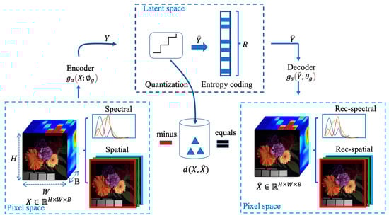
Figure 1. The HSI compression architecture based on transform coding.

In HSI compression, first, the pixel intensities of HSIs are usually modeled as a vector $X\in {ℝ}^{H\times W\times B}$, where H, W and B correspond to the height, width and number of spectral bands, respectively. Then, the vector $X$ is mapped into the latent space via the encoder to produce a dense latent representation $Y$, which is then quantized to remove negligible information and represented as discrete-vector $\widehat{Y}$. Note that most existing transform coding-based methods for HSI compression use orthogonal linear transforms to reduce spectral and spatial correlations. That is, the encoder $g_a$ and decoder $g_s$ are linear functions (e.g., KLT and DWT). In addition, $\widehat{Y}$ can be compressed with entropy coding algorithms (e.g., arithmetic coding [45]) and stored or transmitted in the form of a binary bitstream. On the other hand, we can obtain $\widehat{X}$ after subjecting $\widehat{Y}$ to the decoder. Note that the information loss $d\left(X,\widehat{X}\right)$ (also called distortion) is irreversible; here, $d$ is a metric, such as the mean squared error (MSE), and is used to measure the difference between the original image and the reconstructed image. Thus, errors are inevitable and will affect the quality of image reconstruction. Generally, a higher compression ratio produces more errors (information loss), which leads to a worse quality of the reconstructed image.

To deal with this problem, the tradeoff between the compression ratio and data quality should be considered, which is often described as a rate-distortion optimization problem [46]. The mathematical formulation is usually given as a Lagrangian function L with a Lagrange multiplier $\lambda$ on the distortion [46].

$$R={\mathbb{E}}_{\widehat{Y}~m\left(\widehat{Y}\right)}\left(-lo{g}_{2}p\left(\widehat{Y}\right)\right),$$

(5)

$$ℒ=R+\lambda d\left(X,\widehat{X}\right).$$

(6)

R denotes the estimated average code length of the latent representation, which is generally formulated with a cross-entropy between the entropy model $p\left(\widehat{Y}\right)$ and the marginal distribution $m\left(\widehat{Y}\right)$ of the latents. Note that the entropy model $p\left(\widehat{Y}\right)$ is a prior probability model of the latents known to the entropy coding and is typically assumed to be parametric. The marginal distribution $m\left(\widehat{Y}\right)$ arises from the encoded HSIs and the encoder.

2.3. Neural-Network-Based Image Compression

Neural networks are usually not orthogonal and involve cascades of layers (typically focused on convolution operation). Each layer consists of a linear transform followed by a bias and a nonlinear function $f$.

$$y=f\left(Wx+b\right),$$

(7)

where $x\in {ℝ}^n$ and $y\in {ℝ}^m$ represent the input and output vectors of the layer, respectively, and $W\in {ℝ}^{m\times n}$ and $b\in {ℝ}^m$ are the neural network parameters. Consequently, cascades of $y$ form the transform functions $g_a$ and $g_s$, where ${\varnothing }_g$ and ${\theta }_g$ encapsulate the parameters of the transforms.

The quantized gradients are always zero; hence, a relaxation function is necessary when optimizing the compression network with a gradient descent approach. The additive uniform noise $\mathcal{U}\left(-\frac{1}{2},\frac{1}{2}\right)$ used in [21] is a favorable alternative to quantization, because it can make the network more robust. We also follow this method in this paper, with the details described in Section 3. In addition, once the entropy model $p\left(\widehat{Y}\right)$ is known, the quantized latents $\widehat{Y}$ can be compressed losslessly using entropy coding methods.

Whether the entropy model $p\left(\widehat{Y}\right)$ approaches the marginal distribution $m\left(\widehat{Y}\right)$ is significant for compression performance. As mentioned in [30], a factorized entropy model fails to capture the statistics of the marginal distribution of the latents, and introducing side information can be an elegant approach for reducing this mismatch. Therefore, the hyperprior is proposed to overcome this problem by introducing an additional vector Z to describe the statistical relationship of the latents. Vector Z can be viewed as a prior or a condition of the entropy model. For example, in [30], each latent ${\widehat{Y}}_i$ (where i denotes the ith latent of $\widehat{Y}$) is assumed to accord with a zero-mean Gaussian distribution, where the standard deviation ${\sigma }_i$ is predicted by another encoder-decoder pair $h_a$ and $h_s$. In this case, the objective of Equation (6) can be defined as follows:

$$\begin{array}{c}ℒ=R\left(\widehat{Y}\right)+R\left(\widehat{Z}\right)+\lambda d\left(X,\widehat{X}\right)=\mathbb{E}[-lo{g}_2\left(p\left(\widehat{Y}|\widehat{Z}\right)\right)-\\ lo{g}_2\left(p\left(\widehat{Z}\right)\right)]+\lambda d\left(X,\widehat{X}\right).\end{array}$$

(8)

Note that a uniform noise is employed to relax this problem during training, which yields vectors signed with a tilde. When the loss function becomes continuous, the optimization problem of Equation (8) is similar to something encountered in variational autoencoder (VAE) [47]. The subtlety of the solution of Equation (8) can be conveyed in a Kullback-Leibler divergence between the true posterior $p\left(\tilde{Y},\tilde{Z}|X\right)$ and an approximating density $q\left(\tilde{Y},\tilde{Z}|X\right)$ [30].

$$\begin{array}{c}{D}_{KL}\left[q\left(\tilde{Y},\tilde{Z}|X\right)\left|\right|p\left(\tilde{Y},\tilde{Z}|X\right)\right]={\mathbb{E}}_{\tilde{Y},\tilde{Z}~q}[lo{g}_{2}q\left(\tilde{Y},\tilde{Z}|X\right)-lo{g}_{2}p\left(X|\tilde{Y}\right)-\\ lo{g}_2\left(p\left(\tilde{Y}|\tilde{Z}\right)\right)-lo{g}_2\left(p\left(\tilde{Z}\right)\right)]+constant.\end{array}$$

(9)

The entropy of $q\left(\tilde{Y},\tilde{Z}|X\right)$ in the first term is zero because each latent will be convolved with a standard uniform noise and can be removed from Equation (9). The second term is linked to distortion. When the distortion is Euclidean (such as the MSE metric), $p\left(X|\tilde{Y}\right)$ is Gaussian; otherwise, the distortion is based on an energy function. Finally, the third combined with the fourth term is the total rate of the latent representation that can be modeled as follows.

Due to the lack of prior information, the density of $\tilde{Z}$ is represented as a fully factorized distribution [30].

$$p_{\tilde{Z}|\phi }\left(\tilde{Z}|\phi \right)={{\displaystyle \prod }}_i\left(p_{{\tilde{Z}}_i|{\phi }^{\left(i\right)}}\left({\phi }^{\left(i\right)}\right)\ast \mathcal{U}\left(-\frac{1}{2},\frac{1}{2}\right)\right)\left({\tilde{Z}}_i\right),$$

(10)

where $p_{{\tilde{Z}}_i|{\phi }^{\left(i\right)}}$ denotes a univariate distribution of each component of vector $\tilde{Z}$ with parameter ${\phi }^{\left(i\right)}$, and the cross-entropy of the fourth term can be considered as the side information.

The side information only occupies a small proportion of the total rate. Therefore, the accuracy of the model $p\left(\tilde{Y}|\tilde{Z}\right)$ is significant in reducing the mismatch between the entropy model and marginal distribution. Most existing studies assume this conditional probability distribution to be a zero-mean Gaussian distribution. Later, it was improved with a conditional mean to exploit more structures of the latent representation [25]. Note that all of these methods involve a Gaussian supposition for the latents, but may not fit many real cases. A discretized Gaussian mixed approach was proposed in [26] to increase the flexibility and precision of the entropy model. Although this method can fit each latent more accurately, each latent is represented with several weighted Gaussian models instead of a univariate distribution, which increases the complexity of the entropy model. In this paper, we concentrate on the hyperspectral data and consider a univariate non-Gaussian probability in the compression task.

3. Proposed HSI Compression Framework

3.1. Statistics of the Compressed HSIs

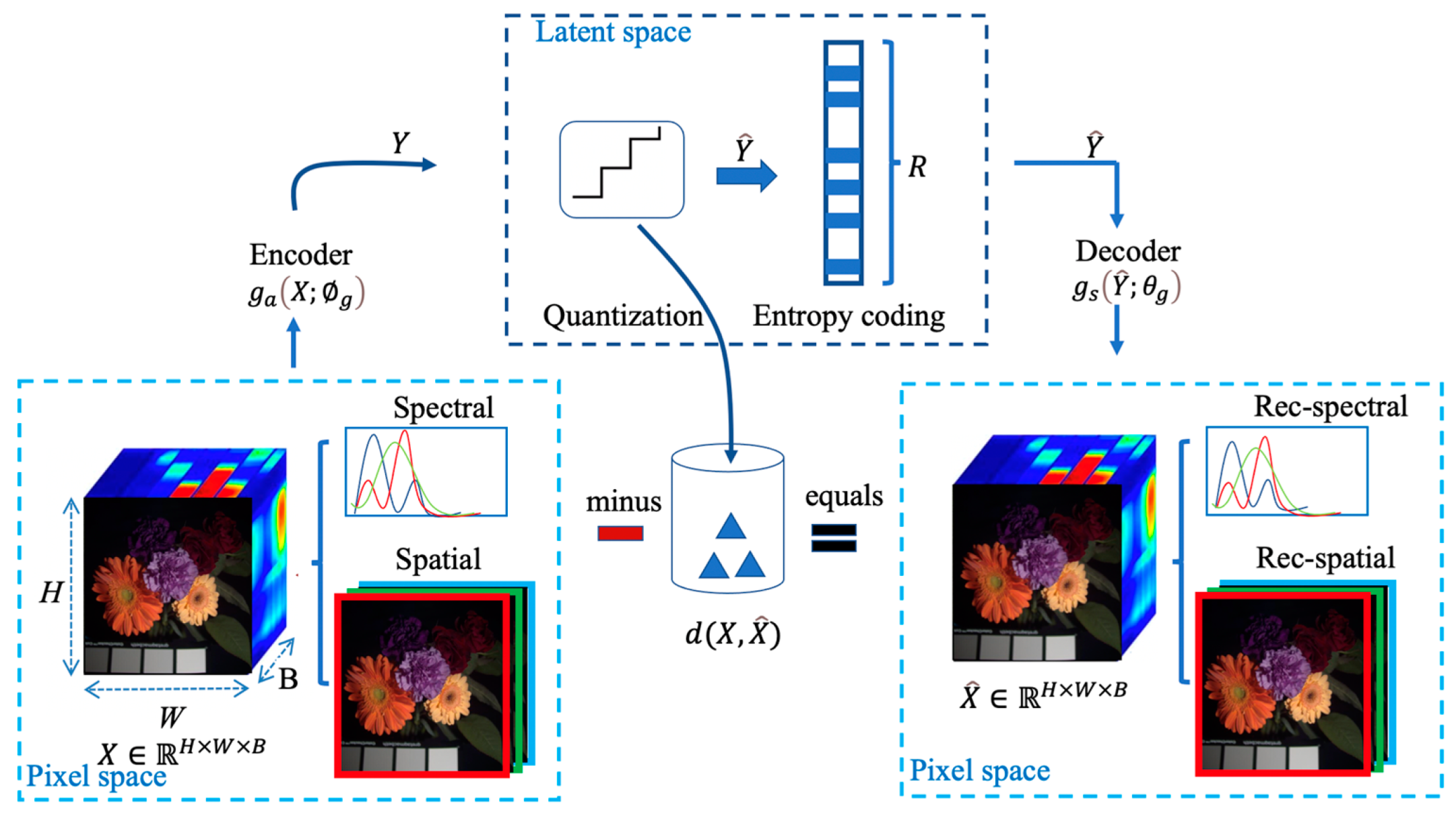
Although there are several parameterized probability models, which one can match the true marginal distribution perfectly is still unknown. We visualize the latents of natural images and HSIs and fit them with some common parameterized probability models, including Gaussian distributions, Student’s T, Laplace distribution and gamma distribution.

The latents are obtained from the same encoder network [30] over four datasets: the Kodak dataset with RGB bands (natural images), two nature HSI datasets (KAIST [48], CAVE [49]) with 31 spectral bands and one remote sensing HSI dataset (ROSIS-Pavia data) with 102 spectral bands (e.g., Pavia University (Pavia_U)). The results are shown in Figure 2.

Figure 2. Different distributions (Gaussian (also called norm) and Student’s T (also simplified to t)) fitted to empirical histograms (blue blocks). The best distribution plot is described with the orange line. (a) Kodak, (b) CAVE, (c) KAIST, (d) Pavia _ U.

In Figure 2, different colors in the legend are sorted by the degree of distribution match, and the orange lines are used to represent the best match. It is clear that the latents of HSIs exhibit striking non-Gaussian behavior as compared with natural images, and Student’s T can achieve a performance competitive with other distributions. Moreover, Student’s T prior in VAEs can provide a more robust density than the Gaussian distribution [42]. These results provide a statistical basis for our Student’s T hyperprior. Therefore, we choose the Student’s T likelihood as the prior in HSI entropy modeling.

3.2. Statistics of the Compressed HSIs Characterized with Student’s T Likelihood

For a given variable set $\tilde{Z}$, the conditional distribution of $\tilde{Y}$ can be expressed as

$$\begin{array}{c}p\left(\tilde{Y}|\tilde{Z}\right)={{\displaystyle \int }}_0^{\infty }gamma\left(\varrho |l\left(\tilde{Z}\right),s\left(\tilde{Z}\right)\right)\mathcal{N}\left(\tilde{Y}|{\mu }_{{\theta }_h}\left(\tilde{Z}\right),{\varrho }^{-1}\right)d\varrho \\ =\frac{\Gamma \left(\frac{v+1}{2}\right)}{\Gamma \left(\frac{v}{2}\right)}{\left(\frac{{\eta }_{{\theta }_h}\left(\tilde{Z}\right)}{\pi v}\right)}^{\frac{1}{2}}{\left[1+\frac{{\eta }_{{\theta }_h}\left(\tilde{Z}\right){\left(\tilde{Y}-{\mu }_{{\theta }_h}\left(\tilde{Z}\right)\right)}^2}{v}\right]}^{-\frac{v+1}{2}}\\ =St(\tilde{Y}|{\mu }_{{\theta }_h}\left(\tilde{Z}\right),{\eta }_{{\theta }_h}\left(\tilde{Z}\right),v),\end{array}$$

(11)

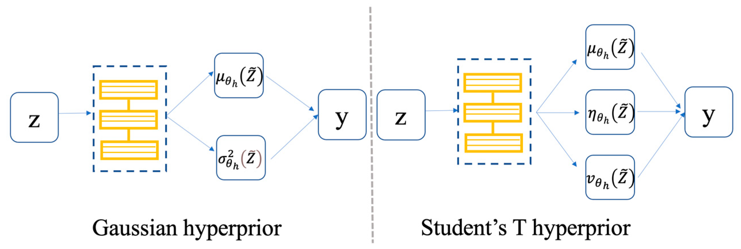
where $\varrho =1/{\sigma }_{{\theta }_h}^2\left(\tilde{Z}\right)$ is the inverse of the variance, $l\left(\tilde{Z}\right)$ and $s\left(\tilde{Z}\right)$ correspond to the shape parameter and the inverse scale parameter of the gamma distribution, respectively, precision ${\eta }_{{\theta }_h}=l\left(\tilde{Z}\right)/s\left(\tilde{Z}\right)$ is similar to $\varrho$ but in some cases not identical, and the degree of freedom $\nu =2l\left(\tilde{Z}\right)$. Similar to the solution of Gaussian parameters in [30] (as shown in Figure 3, left side), we also use a hyperprior network (an encoder-decoder pair $h_a$ and $h_s$) to predict the parameters of Student’s T (as shown in Figure 3, right side), where ${\theta }_h$ denotes the parameters of the hyperprior decoder $h_s$. In this paper, we model the probability of each latent as a zero-mean Student’s T distribution with a precision ${\eta }_{{\theta }_h}\left(\tilde{Z}\right)$ in our framework, that is, the mean ${\mu }_{{\theta }_h}=0$ and ${\eta }_{{\theta }_h}=h_s\left(\tilde{Z};{\theta }_h\right)$ under the condition of a fixed $\nu$ to simplify the network in our experiments.

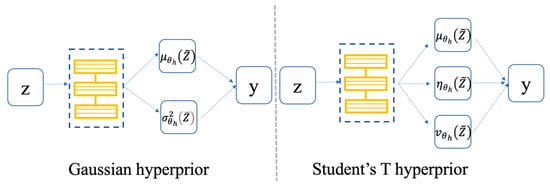
Figure 3. Hyperprior neural network. The left side is the Gaussian hyperprior, which is used to estimate the mean ${\mu }_{{\theta }_h}\left(\tilde{Z}\right)$ and variance ${\sigma }_{{\theta }_h}^2\left(\tilde{Z}\right)$, while the right side is the Student’s T hyperprior, which is used to estimate the mean ${\mu }_{{\theta }_h}\left(\tilde{Z}\right)$, precision ${\eta }_{{\theta }_h}\left(\tilde{Z}\right)$ and the degree of freedom $v_{{\theta }_h}\left(\tilde{Z}\right)$.

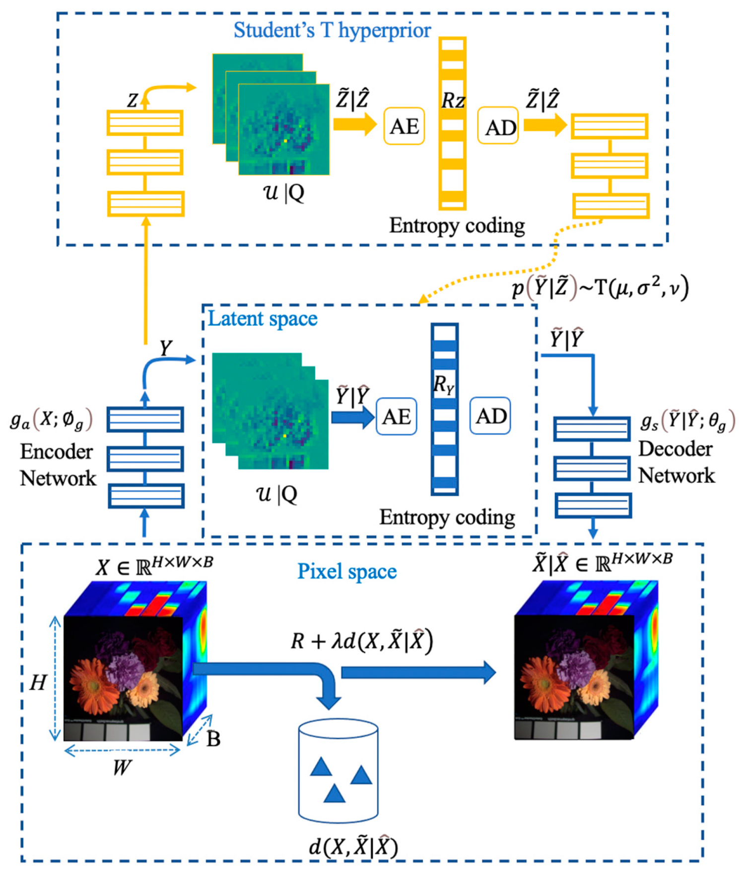
In conclusion, the proposed HSI compression model with the Student’s T hyperprior can be described as in Figure 4. This model is composed of two sub-networks. The core autoencoder (Encoder Network and Decoder Network), also the first sub-network, is used to learn a discrete latent representation of HSIs. The second is implemented to learn an accurate entropy model over quantized latents for entropy coding, where we extend the conditional Gaussian-based model with a conditional Student’s T for entropy modeling. This hypernetwork is used to generate the parameters of the Student’s T, such as the mean and the precision. The optimization problem can be summarized as minimizing the expected rate-distortion loss function defined in Equation (8).

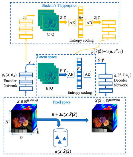
Figure 4. An end-to-end HSI compression model with the Student’s T hyperprior. $\mathcal{U}$|Q corresponds to either additive uniform noise employed during training (yielding vectors signed with a tilde) or rounding during testing (yielding vectors signed with a hat). The architecture of the hyperprior is identical to [30], except that we use a Student’s T likelihood. The details of $g_a$ and $g_s$ are specified in Section 3.3.

To ensure a good match between Student’s T prior $p\left(\tilde{Y}|\tilde{Z}\right)$ and the variational posterior $q\left(\tilde{Y},\tilde{Z}|X\right)$, we apply the same approach as Ballé et al. [30], convolving $p\left(\tilde{Y}|\tilde{Z}\right)$ with a standard uniform to make the continuous-valued latents subject to the uniform when training. Then, the entropy model can be formulated as

$$P\left(\tilde{Y}|\tilde{Z}\right)={{\displaystyle \prod }}_i\left(St({\tilde{Y}}_i|0,{\eta }_i,v)\ast \mathcal{U}\left(-\frac{1}{2},\frac{1}{2}\right)\right)\left({\tilde{Y}}_i\right)=c\left({\tilde{Y}}_i+\frac{1}{2}\right)-c\left({\tilde{Y}}_i-\frac{1}{2}\right),$$

(12)

where i is the location of each latent and $c(.)$ specifies the collective cumulative distribution function (CDF). The cumulative of Student’s T in our experiments is as follows [50].

For $v$ odd and greater than 1:

$$P\left(t_v\right)=\frac{1}{2}+\frac{1}{\pi }\left\{\xi +\left[cos\xi +\frac{2}{3}co{s}^3\xi +\cdots +\frac{\left(2\right)\left(4\right)\dots \left(v-3\right)}{\left(3\right)\left(5\right)\dots \left(v-2\right)}co{s}^{v-2}\xi \right]sin\xi \right\},$$

(13)

$$\begin{array}{c}\mathrm{For}v\mathrm{even}:\hfill \\ \hspace{1em}\hspace{1em}\hspace{1em}\hspace{1em}\hspace{1em}P\left(t_v\right)=\frac{1}{2}+\frac{1}{2}\left[1+\frac{1}{2}co{s}^2\xi +\frac{\left(1\right)\left(3\right)}{\left(2\right)\left(4\right)}co{s}^4\xi +\cdots +\frac{\left(1\right)\left(3\right)\dots \left(v-3\right)}{\left(2\right)\left(4\right)\dots \left(v-2\right)}co{s}^{v-2}\xi \right]sin\xi ,\end{array}$$

(14)

where $\xi =\arctan \left(t_v/\sqrt{\nu }\right)$.

3.3. HSI Compression Network Construction

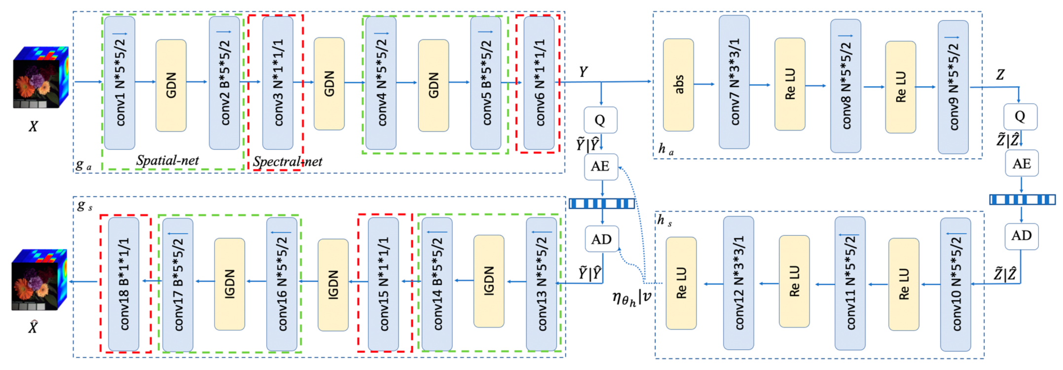
Our HSI compression architecture consists of two main parts. The comprehensive architecture is shown in Figure 5. The left side is the primary encoder-decoder pair ($g_a$ and $g_s$) composed of SS-Nets, which is cascades of convolutions and generalized divisive normalization (GDN) or inverse generalized divisive normalization (IGDN) [38] (here, GDN and IGDN have been proven to be efficient nonlinear functions executing local normalization for the image compression task [21]), while the right side is the hyperprior network, which is identical to [30] but enhanced with a more accurate entropy model using an adjustable Student’s T likelihood as its prior. Here, $h_a$ and $h_s$ are a series of convolutions and rectified linear units, respectively. In addition, Q indicates quantization, AE is the arithmetic encoder, and AD is the arithmetic decoder. Q is implemented using a rounding operation when testing or replaced with a uniform noisy during training, while AE and AD are implemented with a simple binary arithmetic. Note that the convolutions are not restricted; they can be exchanged with residual blocks or dense blocks without changing the fundamental model.

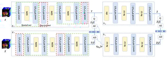
Figure 5. The HSI compression architecture. The green and red boxes, on the left side, represent spatial and spectral networks, respectively. Q indicates quantization, and AE and AD correspond to the arithmetic encoder-decoder pair. For the convolution operation, parameters are described as the number of filters $\times$ kernel size (height $\times$ width)/down-sampling/up-sampling stride (the factor is 2), where <- denotes up-sampling and -> down-sampling. B is the band number of HSIs (in this paper, B = 31 for CAVE and KAIST datasets and B = 102 for ROSIS-Pavia data). N is the number of filters; we find performance gains will stagnate when the number of filters is increased to a certain level, and N = 192 yields a good performance in our experiments.

In order to fully exploit the spatial and spectral correlation, the design of $g_a$ and $g_s$ networks should take the anisotropic characteristic of HSIs into consideration. We design our spatial network (the spatial net circled with a green box in Figure 5) and spectral network (the spectral net circled with a red box in Figure 5) separately. There are two convolutional layers in the spatial network connected with GDN or IGDN. The first layer employs N/B filters with a size of $5\times 5$ and down-sampling/up-sampling with a factor of 2, where B equals the number of spectral bands of HSIs, and N is the number of the filters. The number of output channels of the last layer of the primary encoder is the bottleneck, which determines the components that should be stored. The spectral network employs N/B filters with a size of $1\times 1$. Note that the output channels of the final layer of the primary decoder must be consistent with the band numbers of HSIs to generate identical spectral resolution. The details of hyperparameters can be found in Appendix A.

4. Experiments

We first illustrate the advantage of the proposed spatial and spectral network for the HSI compression task. Then, we find that Student’s T likelihood is more flexible than Gaussian as the degree of freedom changes. Finally, we compare the rate-distortion performance of our model to two commonly used linear transform coding methods and a nonlinear transform method. The neural network-based compression methods are executed on a server equipped with the NVIDIA GeForce RTX 2080Ti graphics card, and the traditional compression methods are implemented in CPU i5-8279@2.4GHz.

4.1. Experimental Datasets

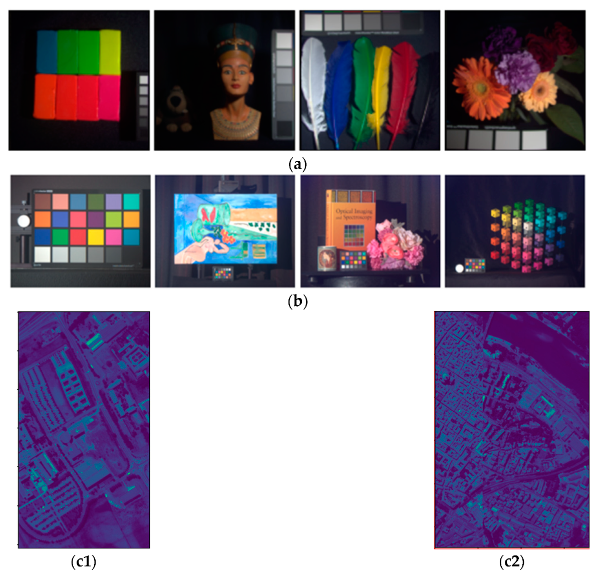
To comprehensively evaluate the proposed HSI compression architecture, we train our models with three datasets of high quality HSIs and test our models without retraining when compressing new HSIs. Specifically, we use two nature HSI datasets (KAIST [48] and CAVE [49]) with 31 spectral bands and one remote sensing HSI dataset (ROSIS-Pavia data) with 102 spectral bands (from Pavia University and Pavia Centre). In order to obtain an effective visualization of different areas, we render the input gray image as a pseudocolor image to visualize different areas so as to meet the requirement of human perception.

4.1.1. CAVE

There are 32 scenes in the CAVE database, which involve a large variety of daily materials and objects. The spatial resolution is 512 × 512, while the 31 spectra at each pixel are reflected at a wavelength step of 10 nm from 400 nm to 700 nm. Some representative thumbnails are shown in Figure 6a.

Figure 6. Representative thumbnails of each dataset. (a) CAVE; (b) KAIST; (c1) Pavia_U (band55); (c2) Pavia_C (band55).

4.1.2. KAIST

The KAIST dataset is a high-resolution database including 30 scenes with a spatial size of 2704 × 3376. The spectral range covers 420–720 nm at a step of 10 nm, thus producing 31 spectra. Some representative thumbnails are shown in Figure 6b.

4.1.3. ROSIS-Pavia

The Pavia database consists of two scenes captured by the ROSIS sensor. Therefore, we call it ROSIS-Pavia in this paper. The first scene is Pavia Centre (Pavia_C), involving 102 spectral bands, with a spatial resolution of 1096 × 715. The second scene is Pavia University, involving 103 spectral bands, with a spatial resolution of 610 × 340. We remove one noise band (call it PaviaU_102) to maintain consistency with the number of bands of the Pavia Centre. We set Pavia_C as the training set and Pavia University as the testing set in the experiments. In the training process, we use the random crop trick to enlarge our training set due to the small samples of Pavia_C. In addition, in order to evaluate the model generalization, we also set the half resolution of Pavia_C as a part of testing set, since there are only two images of ROSIS-Pavia, and scaling Pavia_C to half resolution (named Pavia_C_1/2) can be seen as a data augmentation to enlarge our testing data. The Pavia University and Pavia Centre are shown in Figure 6(c1,c2).

4.2. Experimental Configuration

4.2.1. Metrics

We use bit per pixel per band (bpppb) to evaluate the compression ratio of HSIs and use three common metrics to evaluate the distortion for compression task: PSNR, SSIM [51] and spectral angle mapping (SAM) [52].

Bpppb is evaluated by Equation (5), and the accuracy of the entropy model has a strong effect on this evaluation. In addition, PSNRs for HSIs are calculated as follows in this paper:

$$PSNR=10lo{g}_{10}\frac{ma{x}_b^2}{mse},$$

(15)

where $b\in B$ and B is the number of bands of HSIs, and $ma{x}_b$ denotes the maximum value in this band. In addition, the unit is dB.

For SSIM, we first compute the SSIMs of each band and then average them over the full spectral bands. SAM (represented as degree) is used to describe the angle of the pixels between the reconstructed HSI and the original HSI. Note that large values of PSNR and SSIM imply high spatial fidelity, and small values of SAM reflect high spectral fidelity.

4.2.2. Parameter Setup

In terms of the two nature HSI datasets, we randomly choose 28 HSIs from the CAVE data and 27 HSIs from the KAIST data as the training set (10% as validation) and crop each scene randomly into overlapping $128\times 128$ patches with full spectral bands. For Pavia Centre, we also randomly extract $128\times 128$ overlapping patches for training, and scale a half resolution for testing. The proposed HSI compression architecture is implemented in the TensorFlow framework [30], with eight minibatches at a time. In addition, the Adam stochastic gradient descent algorithm [53] is used in training, with a learning rate of $1\times {10}^{-4}$.

4.2.3. Method in Comparison

First, to illustrate the advantage of the proposed spatial and spectral network for the HSI compression task, we compare with [30] by keeping the entropy model identical. Then, we demonstrate the superiority of Student’s T prior for HSI compression from the spatial and spectral aspects. To further verify the effectiveness of this learned hyperspectral compression approach, we compare it with two representative linear transform coding based HSI compression methods, namely KLT + JPEG2000 [15] and the 3D version set partitioned embedded block (3D SPECK) [54] and a state-of-the-art learned model [25]. For the KLT + JPEG2000 method, a KLT transform is first applied to the spectral dimension, and then JPEG2000 is applied in the spatial domain. Note that JPEG2000 is carried out with Kakadu version 8.0.5 in this paper. For 3D SPECK, the main idea is to employ a 3D DWT to HSIs and then provide a sequence for significant pixels with a block splitting algorithm. Note that 3D SPECK is implemented with QccPack in our experiments. For the learned model [25], we use the open sources provided by the authors.

4.3. Experimental Results

4.3.1. Potential of the SS-Net for HSI Compression

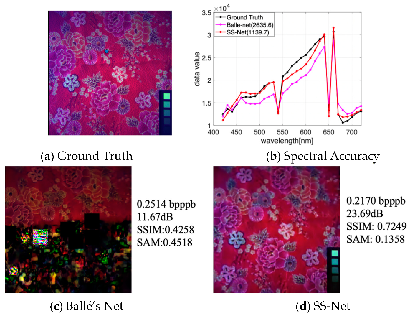
One of the key points of the proposed HSI compression model is the SS-Net, which can be more efficient and robust for spatial and spectral feature extraction, particularly for scenes involving rich texture details. If we just consider the spatial transform (e. g. Ballé’s Net [30]), we may miss some data of HSIs in training, therefore reducing the performance for certain HSIs. Figure 7 shows this problem. There are some data and noise missing in Figure 7c, while the entire spatial information can be reserved in Figure 7d with SS-Net. Both PSNR and SSIM increase by approximately 50%. The SAM reduces by approximately 30%, and the reconstructed spectrum is closer to the ground truth (the red plot (SS-Net) is closer to the black plot in Figure 7b (ground truth represents the original HSI)). Moreover, when the Lagrange multiplier $\lambda$ is set to the same value, SS-Net can achieve a smaller bpppb. Note that the experiments are implemented with the Gaussian prior in the hyperprior.

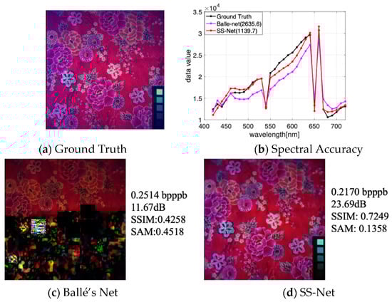
Figure 7. Impact of the SS-Net for HSI compression, false color (composed of bands 25, 10, 1), $\lambda =0.0000001$. (a) is the original spatial domain, also called ground truth; (b) shows the results of the spectral accuracy comparisons for the bule point (169, 243) in the ground truth, and the number in the chart is the value of RMSE (root mean squared error; a small value shows a better spectral accuracy); (c) denotes the reconstructed HSI without considering the difference between the spectral dimension and the spatial domain; (d) represents the reconstructed HSI with SS-Net.

4.3.2. Flexibility of Student’s T Likelihood for HSI Compression

The degree of freedom $\nu$ is a significant parameter to determine the shape of the Student’s T. To reduce the number of training models, we evaluate the influence of the degrees of freedom by observing the compression performance at a specific bpppb. Table 1 shows the results of CAVE and KAIST datasets as $\nu$ varies.

Table 1. Rate-distortion performance of various degrees of freedom for a particular bit rate. The comparatively ideal choice is marked in bold. Bpppb represents bit per pixel per band.

Dataset	Methods		bpppb	PSNR	SSIM	SAM
CAVE	Gaussian		0.6394	33.48	0.8985	0.2382
	Student’s T	$\nu$ = 15	0.6404	36.05	0.9558	0.1453
		$\mathit{\nu }$= 17	0.6023	36.25	0.9555	0.1381
		$\nu$ = 19	0.6357	36.23	0.9563	0.1370
		$\nu$ = 20	0.6319	36.05	0.9548	0.1479
		$\nu$ = 21	0.6024	34.76	0.9459	0.1559
		$\nu$ = 23	0.6245	35.87	0.9550	0.1456
KAIST	Gaussian		0.4680	41.27	0.9782	0.0958
	Student’s T	$\nu$ = 15	0.4294	42.48	0.9826	0.0755
		$\nu$ = 17	0.4432	42.51	0.9819	0.0806
		$\mathit{\nu }$= 18	0.4390	42.86	0.9829	0.0677
		$\nu$ = 20	0.4371	42.84	0.9825	0.0728
		$\nu$ = 21	0.4041	42.42	0.9812	0.0826
		$\nu$ = 24	0.4818	41.74	0.9785	0.0858

An examination of the results presented in Table 1 shows that as $\nu$ changes, the compression performance at a specific rate first increases and then decreases. Moreover, most of the Student’s T priors (with different values of $\nu$) obtain a better result than the Gaussian prior, and this flexible characteristic is beneficial for obtaining an optimal compression performance if $\nu$ is set appropriately. We can select various values of $\nu$ at each rate to obtain the optimal rate-distortion performance. However, in the training process, we find the best choice of $\nu$ for a specific dataset is almost the same at different rates. Therefore, to simplify the training process, we choose an identical $\nu$ for all rates in a specific dataset. Note that the value of $\nu$ may be different for various datasets. For example, we choose $\nu =17$ for CAVE and $\nu =18$ for KAIST after a comprehensive analysis of three distortion metrics.

4.3.3. Rate-Distortion Performance Analysis

In addition, the average rate-distortion performance for CAVE and KAIST datasets are shown in Figure 8 and Figure 9, where Figure 8 describes the rate-distortion curves and Figure 9 shows the reconstructed visualization of the individual HSIs. For ROSIS-Pavia, we find that a large number of bands reduces the training speed. Therefore, we just train four separate models, two relatively low bit rates and two relatively high bit rates, where two models are based on the Gaussian prior and two models are based on the Student’s T prior. The rate-distortion results are shown in Table 2 and Table 3, where Table 2 corresponds to a low bit rate and Table 3 corresponds to a high bit rate. Figure 10 shows the reconstructed visualization of the individual HSIs at low bit rates (the quantitative results are shown in Table 2).

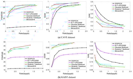
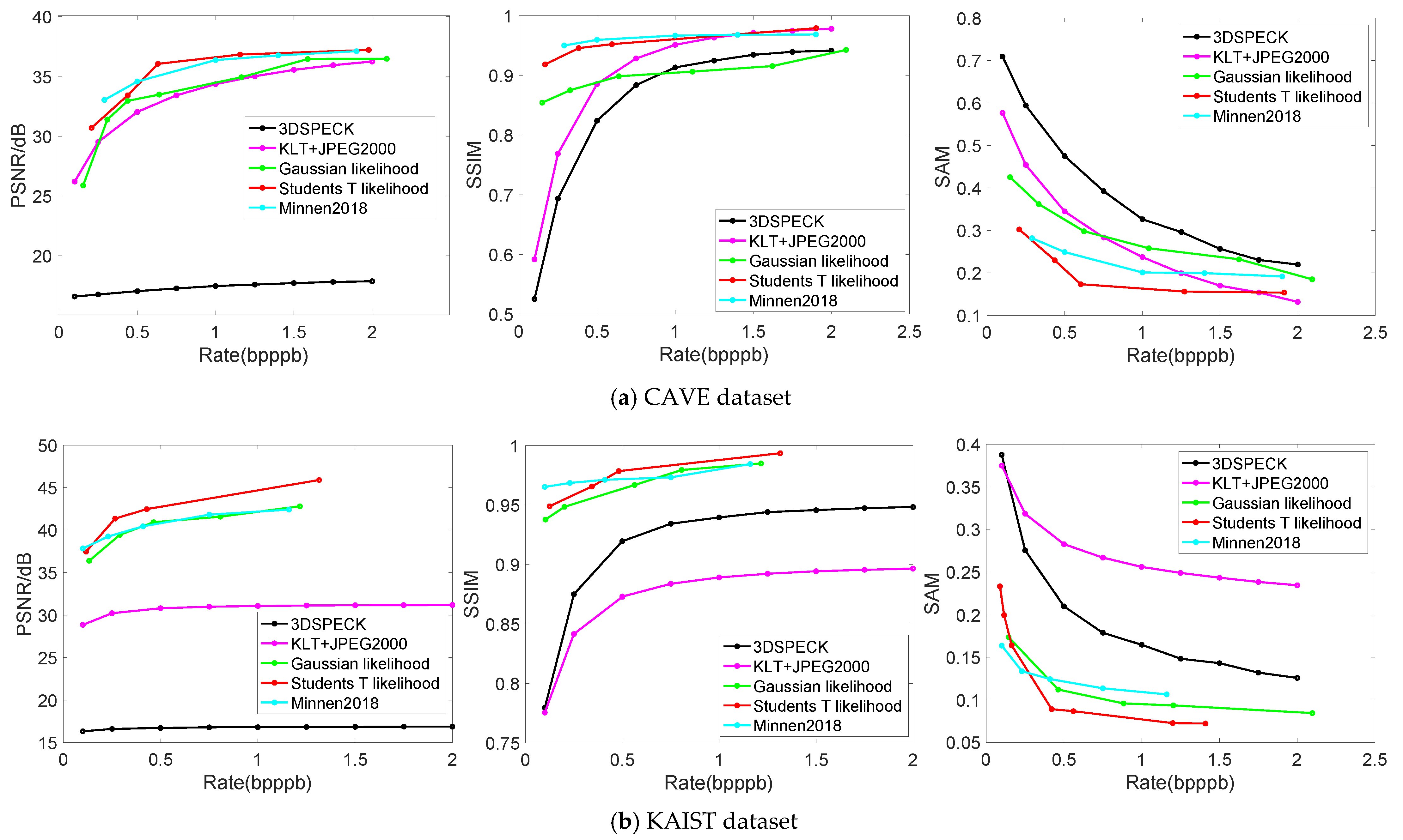
Figure 8. Rate-distortion performance displayed over CAVE and KAIST datasets. The left plots show average PSNRs. The middle plots show average SSIMs, ranging from zero and one. The right plots show average SAMs. (a) Rate-distortion performance displayed over CAVE; (b) Rate-distortion performance displayed over KAIST.

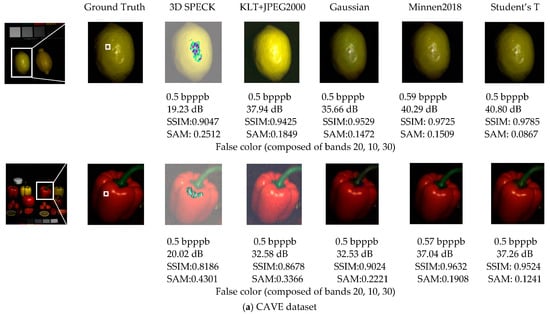
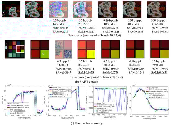
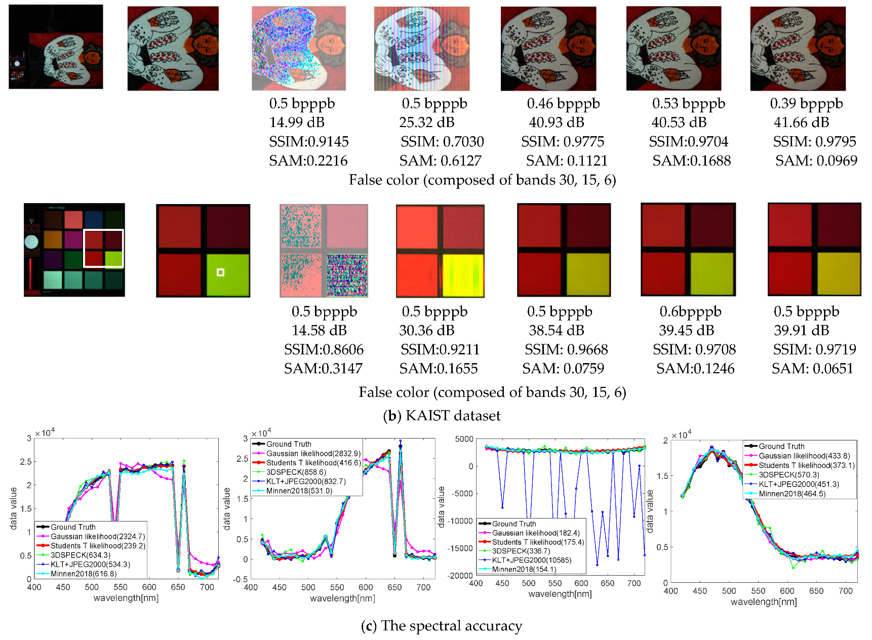
Figure 9. The spatial and spectral fidelity of CAVE and KAIST datasets. The top four rows show the reconstructions of the spatial domain, and quantitative values of distortion, PSNRs, SSIMs and SAMs are shown below. The false color bands are given under the metrics. The last row shows the spectral accuracy, corresponding to the top four images in turn. The plot legends show the reconstructed spectral accuracy of the white patches on ground truth, measured with RMSEs in parenthesis (a small value denotes a better spectral accuracy).

Table 2. Rate-distortion performance for relatively low bit rates; the comparatively ideal choice is marked in bold ($\lambda =\mathbf{0.000005}$).

Dataset	Methods	bpppb	$\mathbf{PSNR}$	SSIM	$\mathbf{SAM}$
PaviaU_102	Student’s T likelihood	0.22	27.86	0.9760	0.1131
	Gaussian likelihood	0.24	26.99	0.9713	0.1278
	KLT+ JPEG2000	0.25	26.23	0.9629	0.1964
	3D SPECK	0.25	25.53	0.9559	0.2128
Pavia_C_1/2	Student’s T likelihood	0.22	28.59	0.9774	0.1261
	Gaussian likelihood	0.23	28.56	0.9770	0.1280
	KLT+ JPEG2000	0.25	25.49	0.9528	0.2949
	3D SPECK	0.25	25.09	0.9471	0.3192

Table 3. Rate-distortion performance for relatively high bit rates; the comparatively ideal choice is marked in bold ($\lambda =\mathbf{0.00005}$).

Dataset	Methods	bpppb	$\mathbf{PSNR}$	SSIM	$\mathbf{SAM}$
PaviaU_102	Student’s T likelihood	0.98	32.85	0.9926	0.0785
	Gaussian likelihood	1.04	32.22	0.9917	0.0831
	KLT + JPEG2000	1.00	32.72	0.9921	0.1107
	3D SPECK	1.00	31.76	0.9897	0.1341
Pavia_C_1/2	Student’s T likelihood	0.91	33.68	0.9934	0.0885
	Gaussian likelihood	0.93	33.38	0.9929	0.0938
	KLT + JPEG2000	1.00	31.28	0.9887	0.2024
	3D SPECK	1.00	30.95	0.9873	0.2265

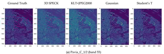
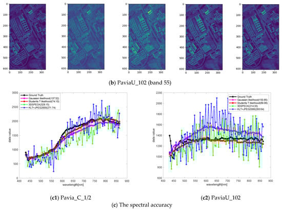
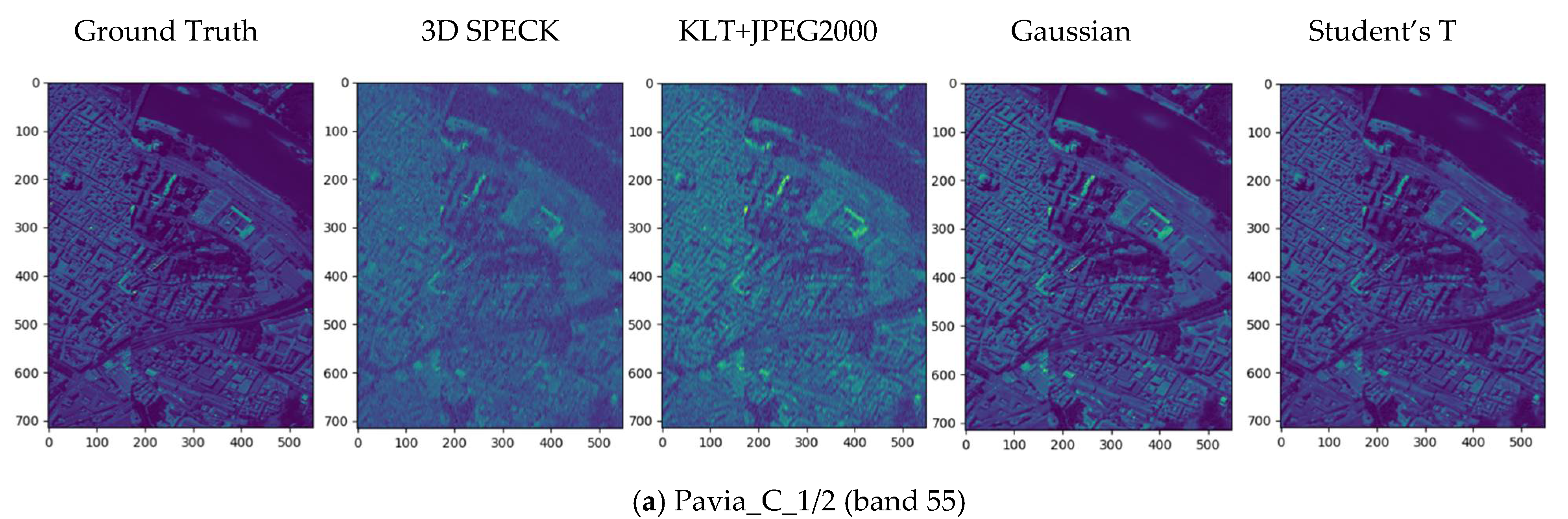
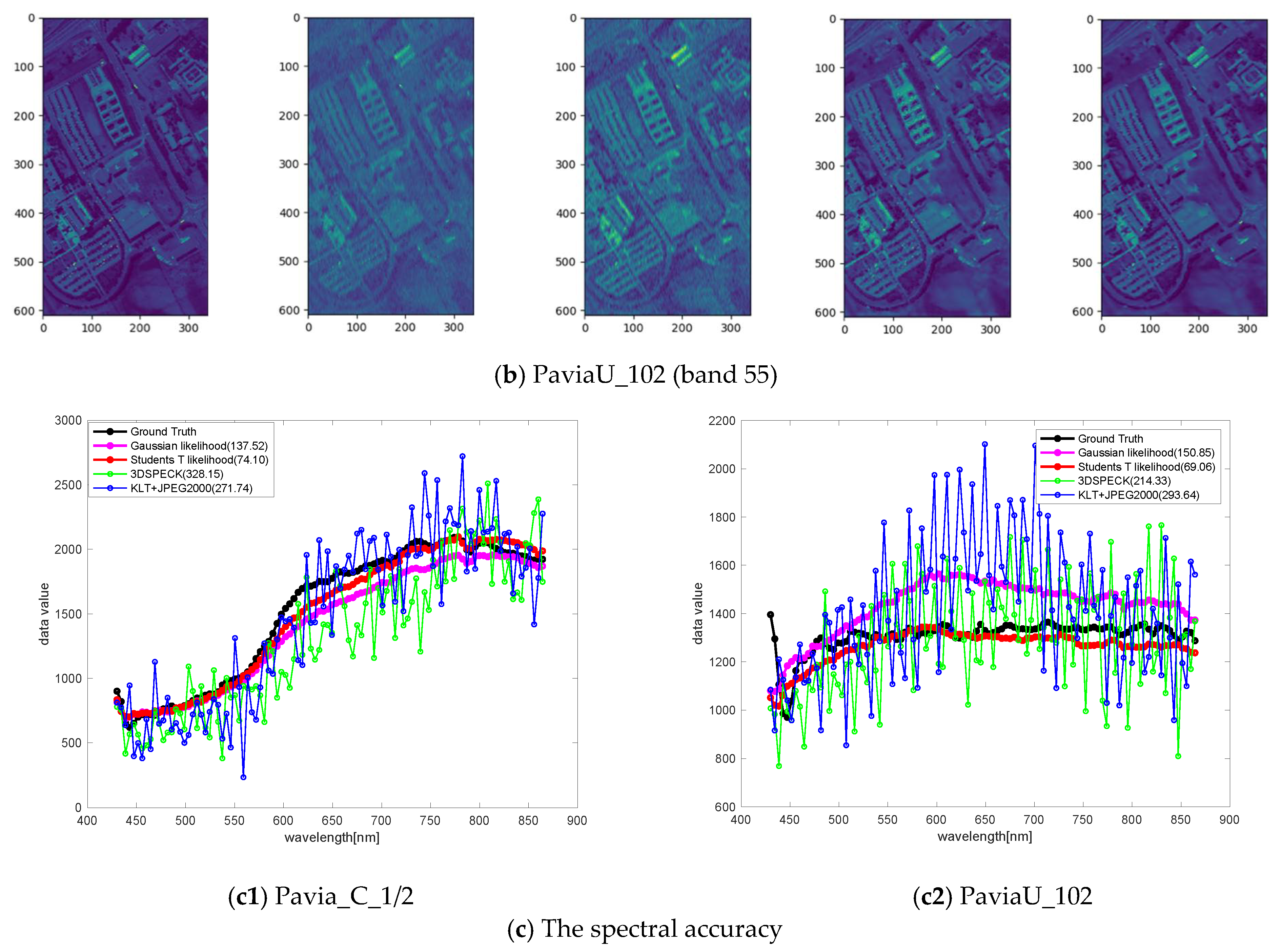
Figure 10. The spatial and spectral fidelity of the ROSIS-Pavia dataset for relatively low bit rates. The first row shows the results of Pavia_C_1/2, while the second row shows the results of PaviaU_102. The visualization of the spatial domain shows the reconstructed quality of band 55. The last row shows the spectral accuracy of the white patches on ground truth, measured with RMSEs in parenthesis. We also show another four HSI dataset comparisons in Appendix B to demonstrate the superiority of our method for HSI compression across different spectral and spatial resolutions and sensors.

Rate-distortion performance with CAVE dataset. The average rate-distortion curves of the CAVE dataset (Figure 8a) show that the nonlinear transform coding methods can achieve competitive performance with the state-of-the-art linear transform coding methods (e.g., KLT+JPEG2000) and outperform them at low bit rates in three distortion metrics, where the Student’s T prior-based models can achieve competitive performance with Minnen (2018) [25], without the context model and the mean parameter (a parameter of entropy model) provided by [25]. Compared with linear transform coding methods, this characteristic is more striking when observing the reconstructed individual images in Figure 9a. Both 3D SPECK and KLT+JPEG2000 generate visual artifacts (noise or transform artifacts) in the spatial domain and provide poor spectral accuracy, while the proposed model using Student’s T hyperprior outperforms all of the reconstructed HSIs with respect to both the spatial domain and spectral accuracy.

Rate-distortion performance with KAIST dataset. The average rate-distortion curves of the KAIST dataset (Figure 8b) show that the nonlinear transform coding methods can significantly outperform the state-of-the-art linear transform coding methods on three distortion metrics. This is not surprising because the spatial resolution of individual KAIST scenes is almost 35 times higher than that of CAVE data, and a large percentage of training patches will lead to good testing performance. In addition, an examination of the reconstructed individual images in Figure 9b shows that both 3D SPECK and KLT + JPEG2000 generate obvious visual artifacts (mainly noise) in the spatial domain and provide poor spectral accuracy, while the learned models outperform all the reconstructed HSIs both in spatial domain and spectral accuracy. The Student’s T prior-based models also perform better than other learned models overall.

Rate-distortion performance with ROSIS-Pavia dataset. In the experiments, we find the rate-distortion performance is better when $\nu =17$. The results illustrate the efficiency and effectiveness of the proposed compression model from the spatial domain and the spectral accuracy. First, the results presented in Table 2 and Table 3 show that the learned models in the Pavia_C_1/2 scene are significantly better than the state-of-the-art linear transform coding methods due to the similar statistics between the training set and the testing set. This characteristic may provide a solution for low-resolution HSI compression. This means training with a high-resolution HSI and testing with its counterpart low-resolution HSI. In terms of the PaviaU_102 scene, the learned models also surpass linear transform coding methods, especially in spectral accuracy under the SAM distortion metric. Figure 10 visualizes the reconstructions of the Pavia_C_1/2 and PaviaU_102 scenes in Table 2 from the spatial domain and the spectral accuracy. The first row shows the comparison results of Pavia_C_1/2, while the second row shows PaviaU_102. Both rows exhibit a color distortion in the spatial domain when HSIs are compressed with the linear transform coding methods, which means that there may be a spectral distortion in the reconstructions. The results show that the learned models have the advantage of retaining the spectral information and achieve better spectral accuracy. The spectral curves in the last plots (the red line (the Student’s T hyperprior) fits to the ground truth (the black line) better), and the distortion measured with SAMs both clearly demonstrate this point.

4.4. Discussion

A spatial-spectral block, involving a spatial net and a spectral net, is developed as the basis component of the core autoencoder, which resembles the pseudo-3D idea [48], consistent with anisotropic hyperspectral cubes. This nonlinear compression architecture possesses a more powerful representation capability than traditional linear transform codecs due to the non-Gaussian characteristic of HSIs. Moreover, we augment this with a more flexible and accurate entropy model by introducing Student’s T distribution over the latents for entropy coding. Like all the deep-learning based methods, our model can be optimized end-to-end with rate and distortion losses. From experiments, we find that the learned models may exhibit high potential if the training set is sufficiently diverse or the compressed HSIs have statistics similar to the training set. Otherwise, the model may lead to a suboptimal performance in some datasets. We will focus on this in our future research.

5. Conclusions

We propose an end-to-end network architecture for the hyperspectral compression task, which not only involves particular characteristics of HSIs, but also embeds an accurate entropy model. First, an SS-Net is designed to match the anisotropic characteristic of HSIs to capture a more powerful latent representation. Then, a Student’s T hyperprior is proposed to reduce the mismatch between the entropy model and latent representation, since the latents exhibit striking non-Gaussian characteristics, and an inaccurate or unmatched prior of the latent representation can lead to an inexact rate estimation. The summarized results illustrate that our method displays better rate-distortion performance than the state-of-the-art linear transform coding methods, which suffer from issues with visual artifacts at low bit rates.

Our study verifies the potential of ANNs for the HSI compression task. The excellent rate-distortion performance over the low-resolution remote sensing HSI dataset can provide convenient storage and transmission for some low-resolution HSI tasks (e.g., HSI fusion). To some extent, our HSI compression method may reduce the impact on the accuracy of other HSI tasks, as our Student’s T prior based models are considerable compared with other compression methods. Although the choice of the degree of freedom increases the flexibility of the entropy model, it also brings a difficulty in selecting the best value, as we fix it in our experiments. In addition, our model may not match the performance of carefully optimized traditional compression methods due to the domain shift between the training set and the testing set. Therefore, the construction of a model that can quickly adapt to different HSI compression tasks and achieve an optimal rate-distortion performance needs to be performed in the future.

References

- Paoletti, M.E.; Haut, J.M.; Plaza, J.; Plaza, A. Deep Learning Classifiers for Hyperspectral Imaging: A Review. ISPRS J. Photogramm. 2019, 158, 279–317. [Google Scholar] [CrossRef]
- Kim, M.H.; Harvey, T.A.; Kittle, D.S.; Rushmeier, H.; Dorsey, J.; Prum, R.O.; Brady, D.J. 3D Imaging Spectroscopy for Measuring Hyperspectral Patterns on Solid Objects. ACM Trans. Graph. Tog. 2012, 31, 38. [Google Scholar] [CrossRef]
- Nguyen, H.V.; Banerjee, A.; Chellappa, R. Tracking via Object Reflectance Using a Hyperspectral Video Camera. In Proceedings of the 2010 IEEE Computer Society Conference on Computer Vision and Pattern Recognition—Workshops, San Francisco, CA, USA, 13–18 June 2010; pp. 44–51. [Google Scholar] [CrossRef]
- Pan, Z.; Healey, G.; Prasad, M.; Tromberg, B. Face Recognition in Hyperspectral Images. IEEE Trans. Pattern Anal. 2003, 25, 1552–1560. [Google Scholar] [CrossRef]
- Qu, Y.; Qi, H.; Kwan, C. Unsupervised Sparse Dirichlet-Net for Hyperspectral Image Super-Resolution. In Proceedings of the 2018 IEEE/CVF Conference on Computer Vision and Pattern Recognition, Salt Lake City, UT, USA, 18–23 June 2018; pp. 2511–2520. [Google Scholar] [CrossRef] [Green Version]
- Christophe, E.; Mailhes, C.; Duhamel, P. Hyperspectral Image Compression: Adapting SPIHT and EZW to Anisotropic 3-D Wavelet Coding. IEEE Trans. Image Process. 2008, 17, 2334–2346. [Google Scholar] [CrossRef] [Green Version]
- Penna, B.; Tillo, T.; Magli, E.; Olmo, G. Transform Coding Techniques for Lossy Hyperspectral Data Compression. IEEE Trans. Geosci. Remote. 2007, 45, 1408–1421. [Google Scholar] [CrossRef]
- Taubman, D.S.; Marcellin, M.W. JPEG2000 Image Compression Fundamentals, Standards and Practice; Springer: Boston, MA, USA, 2002; pp. 209–230. [Google Scholar] [CrossRef]
- Khelifi, F.; Bouridane, A.; Kurugollu, F. Joined Spectral Trees for Scalable SPIHT-Based Multispectral Image Compression. IEEE Trans. Multimedia 2008, 10, 316–329. [Google Scholar] [CrossRef]
- Hou, Y.; Liu, G. Hyperspectral Image Lossy-to-Lossless Compression Using the 3D Embedded ZeroBlock Coding Alogrithm. In Proceedings of the 2008 International Workshop on Earth Observation and Remote Sensing Applications, Beijing, China, 30 June–2 July 2008; pp. 1–6. [Google Scholar] [CrossRef]
- Karami, A.; Beheshti, S.; Yazdi, M. Hyperspectral Image Compression Using 3d Discrete Cosine Transform and Support Vector Machine Learning. In Proceedings of the 2012 11th International Conference on Information Science, Signal Processing and their Applications (ISSPA), Montreal, QC, Canada, 2–5 July 2012; pp. 809–812. [Google Scholar] [CrossRef]
- Karami, A.; Yazdi, M.; Mercier, G. Compression of Hyperspectral Images Using Discerete Wavelet Transform and Tucker Decomposition. IEEE J. Sel. Top. Appl. 2012, 5, 444–450. [Google Scholar] [CrossRef]
- Schelkens, P.; Munteanu, A.; Tzannes, A.; Brislawn, C. JPEG2000. Part 10. Volumetric Data Encoding. In Proceedings of the 2006 IEEE International Symposium on Circuits and Systems, Kos, Greece, 21–24 May 2006; p. 3877. [Google Scholar] [CrossRef]
- Christophe, E.; Léger, D.; Mailhes, C. Quality Criteria Benchmark for Hyperspectral Imagery. IEEE Trans. Geosci. Remote. 2005, 43, 2103–2114. [Google Scholar] [CrossRef] [Green Version]
- Du, Q.; Fowler, J.E. Hyperspectral Image Compression Using JPEG2000 and Principal Component Analysis. IEEE Geosci. Remote. S 2007, 4, 201–205. [Google Scholar] [CrossRef]
- Fu, C.; Yi, Y.; Luo, F.; Du, B. Hyperspectral Image Compression Based on Simultaneous Sparse Representation and General-Pixels. Pattern Recogn. Lett. 2018, 116, 65–71. [Google Scholar] [CrossRef]
- Kwan, C.; Larkin, J. Perceptually Lossless Compression for Mastcam Multispectral Images: A Comparative Study. J. Signal. Inf. Process. 2019, 10, 139–166. [Google Scholar] [CrossRef] [Green Version]
- Kwan, C.; Larkin, J. New Results in Perceptually Lossless Compression of Hyperspectral Images. J. Signal. Inf. Process. 2019, 10, 96–124. [Google Scholar] [CrossRef] [Green Version]
- Chakrabarti, A.; Zickler, T. Statistics of Real-World Hyperspectral Images. In Proceedings of the CVPR 2011, Colorado Springs, CO, USA, 20–25 June 2011; pp. 193–200. [Google Scholar] [CrossRef] [Green Version]
- Lee, J.; Cho, S.; Beack, S.-K. Context-Adaptive Entropy Model for End-to-End Optimized Image Compression. arXiv 2018, arXiv:1809.10452. [Google Scholar]
- Ballé, J.; Laparra, V.; Simoncelli, E.P. End-to-End Optimized Image Compression. In Proceedings of the 5th International Conference on Learning Representations, Toulon, France, 24–26 April 2017. [Google Scholar]
- Golinski, A.; Pourreza, R.; Yang, Y.; Sautiere, G.; Cohen, T.S. Feedback Recurrent Autoencoder for Video Compression. arXiv 2020, arXiv:2004.04342. [Google Scholar]
- Mentzer, F.; Toderici, G.; Tschannen, M.; Agustsson, E. High-Fidelity Generative Image Compression. arXiv 2020, arXiv:2006.09965. [Google Scholar]
- Toderici, G.; Vincent, D.; Johnston, N.; Hwang, S.J.; Minnen, D.; Shor, J.; Covell, M. Full Resolution Image Compression with Recurrent Neural Networks. In Proceedings of the 2017 IEEE Conference on Computer Vision and Pattern Recognition (CVPR), Honolulu, HI, USA, 21–26 July 2017; pp. 435–5443. [Google Scholar] [CrossRef] [Green Version]
- Minnen, D.; Ballé, J.; Toderici, G. Joint Autoregressive and Hierarchical Priors for Learned Image Compression. arXiv 2018, arXiv:1809.02736. [Google Scholar]
- Cheng, Z.; Sun, H.; Takeuchi, M.; Katto, J. Learned Image Compression with Discretized Gaussian Mixture Likelihoods and Attention Modules. In Proceedings of the 2020 IEEE/CVF Conference on Computer Vision and Pattern Recognition (CVPR), Seattle, WA, USA, 13–19 June 2020; pp. 7936–7945. [Google Scholar] [CrossRef]
- Cai, J.; Cao, Z.; Zhang, L. Learning a Single Tucker Decomposition Network for Lossy Image Compression With Multiple Bits-per-Pixel Rates. IEEE Trans. Image Process. 2020, 29, 3612–3625. [Google Scholar] [CrossRef]
- Mentzer, F.; Agustsson, E.; Tschannen, M.; Timofte, R.; Gool, L.V. Practical Full Resolution Learned Lossless Image Compression. In Proceedings of the 2019 IEEE/CVF Conference on Computer Vision and Pattern Recognition (CVPR), Long Beach, CA, USA, 15–20 June 2019; pp. 10621–10630. [Google Scholar] [CrossRef] [Green Version]
- Choi, Y.; El-Khamy, M.; Lee, J. Variable Rate Deep Image Compression with a Conditional Autoencoder. In Proceedings of the 2019 IEEE/CVF Conference on Computer Vision and Pattern Recognition (CVPR), Long Beach, CA, USA, 15–20 June 2019; pp. 3146–3154. [Google Scholar] [CrossRef] [Green Version]
- Ballé, J.; Minnen, D.; Singh, S.; Hwang, S.J.; Johnston, N. Variational Image Compression with a Scale Hyperprior. arXiv 2018, arXiv:1802.01436. [Google Scholar]
- Liu, H.; Chen, T.; Shen, Q.; Yue, T.; Ma, Z. Deep Image Compression via End-to-End Learning. arXiv 2018, arXiv:1806.01496. [Google Scholar]
- Chen, T.; Liu, H.; Ma, Z.; Shen, Q.; Cao, X.; Wang, Y. End-to-End Learnt Image Compression via Non-Local Attention Optimization and Improved Context Modeling. IEEE Trand. Image Process. 2021, 30, 3179–3191. [Google Scholar] [CrossRef]
- Guo, Z.; Wu, Y.; Feng, R.; Zhang, Z.; Chen, Z. 3-D Context Entropy Model for Improved Practical Image Compression. In Proceedings of the 2020 IEEE/CVF Conference on Computer Vision and Pattern Recognition Workshops (CVPRW), Seattle, WA, USA, 14–19 June 2020; pp. 20–523. [Google Scholar] [CrossRef]
- Li, M.; Zuo, W.; Gu, S.; You, J.; Zhang, D. Learning Content-Weighted Deep Image Compression. IEEE Trans. Pattern Anal. 2019, 43, 3446–3461. [Google Scholar] [CrossRef] [Green Version]
- Hinton, G.E.; Salakhutdinov, R.R. Reducing the Dimensionality of Data with Neural Networks. Science 2006, 313, 504–507. [Google Scholar] [CrossRef] [PubMed] [Green Version]
- Theis, L.; Shi, W.; Cunningham, A.; Huszár, F. Lossy Image Compression with Compressive Autoencoders. arXiv 2017, arXiv:1703.00395. [Google Scholar]
- Habibian, A.; Rozendaal, T.; van Tomczak, J.M.; Cohen, T.S. Video CompressionWith Rate-Distortion Autoencoders. In Proceedings of the 2019 IEEE/CVF International Conference on Computer Vision (ICCV), Seoul, Korea, 27 October–2 November 2019; pp. 7032–7041. [Google Scholar] [CrossRef] [Green Version]
- Ballé, J.; Laparra, V.; Simoncelli, E.P. Density Modeling of Images Using a Generalized Normalization Transformation. arXiv 2015, arXiv:1511.06281. [Google Scholar]
- Mentzer, F.; Agustsson, E.; Tschannen, M.; Timofte, R.; Gool, L.V. Conditional Probability Models for Deep Image Compression. In Proceedings of the 2018 IEEE/CVF Conference on Computer Vision and Pattern Recognition, Salt Lake City, UT, USA, 18–23 June 2018; pp. 4394–4402. [Google Scholar] [CrossRef] [Green Version]
- Johnston, N.; Vincent, D.; Minnen, D.; Covell, M.; Singh, S.; Chinen, T.; Hwang, S.J.; Shor, J.; Toderici, G. Improved Lossy Image Compression with Priming and Spatially Adaptive Bit Rates for Recurrent Networks. In Proceedings of the 2018 IEEE/CVF Conference on Computer Vision and Pattern Recognition, Salt Lake City, UT, USA, 18–23 June 2018; pp. 4385–4393. [Google Scholar] [CrossRef] [Green Version]
- Wainwright, M.J.; Simoncelli, E.P. Scale Mixtures of Gaussians and the Statistics of Natural Images. Adv. Neural Inf. Process. Syst. 1999, 12, 855–861. [Google Scholar]
- Takahashi, H.; Iwata, T.; Yamanaka, Y.; Yamada, M.; Yagi, S. Student-t Variational Autoencoder for Robust Density Estimation. In Proceedings of the Twenty-Seventh International Joint Conference on Artificial Intelligence, Stockholm, Sweden, 13–19 July 2018; pp. 2696–2702. [Google Scholar] [CrossRef] [Green Version]
- Abiri, N.; Ohlsson, M. Variational Auto-Encoders with Student’s t-Prior. arXiv 2020, arXiv:2004.02581. [Google Scholar]
- Goyal, V.K. Theoretical Foundations of Transform Coding. IEEE Signal. Proc. Mag. 2001, 18, 9–21. [Google Scholar] [CrossRef] [Green Version]
- Rissanen, J.; Langdon, G. Universal Modeling and Coding. IEEE Trans. Inf. Theory 1981, 27, 12–23. [Google Scholar] [CrossRef]
- Shoham, Y.; Gersho, A. Efficient Bit Allocation for an Arbitrary Set of Quantizers (Speech Coding). IEEE Trans. Acoust. Speech Signal. Process. 1988, 36, 1445–1453. [Google Scholar] [CrossRef] [Green Version]
- Kingma, D.P.; Welling, M. Auto-Encoding Variational Bayes. arXiv 2013, arXiv:1312.6114. [Google Scholar]
- Choi, I.; Jeon, D.S.; Nam, G.; Gutierrez, D.; Kim, M.H. High-Quality Hyperspectral Reconstruction Using a Spectral Prior. ACM Trans. Graph. 2017, 36, 1–13. [Google Scholar] [CrossRef] [Green Version]
- Yasuma, F.; Mitsunaga, T.; Iso, D.; Nayar, S.K. Generalized Assorted Pixel Camera: Postcapture Control of Resolution, Dynamic Range, and Spectrum. IEEE Trans. Image Process. 2010, 19, 2241–2253. [Google Scholar] [CrossRef] [Green Version]
- Elderton, W.P.; Johnson, N.L. Systems of Frequency Curves; Cambridge University: Cambridge, UK, 1969; pp. 110–121. [Google Scholar] [CrossRef]
- Wang, Z.; Simoncelli, E.P.; Bovik, A.C. Multi-Scale Structural Similarity for Image Quality Assessment. In Proceedings of the Thrity-Seventh Asilomar Conference on Signals, Systems & Computers, Pacific Grove, CA, USA, 9–12 November 2003; pp. 1398–1402. [Google Scholar] [CrossRef] [Green Version]
- Kruse, F.A.; Lefkoff, A.B.; Boardman, J.W.; Heidebrecht, K.B.; Shapiro, A.T.; Barloon, P.J.; Goetz, A.F.H. The Spectral Image Processing System (SIPS)—Interactive Visualization and Analysis of Imaging Spectrometer Data. Remote Sens. Environ. 1993, 44, 145–163. [Google Scholar] [CrossRef]
- Kingma, D.P.; Ba, J. Adam: A Method for Stochastic Optimization. arXiv 2014, arXiv:1412.6980. [Google Scholar]
- Tang, X.; Pearlman, W.A. Lossy-to-Lossless Block-Based Compression of Hyperspectral Volumetric Data. In Proceedings of the 2004 International Conference on Image Processing, Singapore, 24–27 October 2004; pp. 3283–3286. [Google Scholar] [CrossRef]
Publisher’s Note: MDPI stays neutral with regard to jurisdictional claims in published maps and institutional affiliations. |
© 2021 by the authors. Licensee MDPI, Basel, Switzerland. This article is an open access article distributed under the terms and conditions of the Creative Commons Attribution (CC BY) license (https://creativecommons.org/licenses/by/4.0/).