The Intriguing Structure of Stripes in GRACE Geopotential Models

Abstract

Geopotential models derived from Gravity Recovery and Climate Experiment (GRACE) mission measurements are significantly obscured by the presence of a systematic artifact, known as longitudinal stripes. Based on our previous work (Peidou and Pagiatakis, 2020) we provide an in-depth analysis of the latitudinal sampling characteristics of GRACE and we reveal the intriguing sampling mechanism that creates sub-Nyquist artifacts (stripes). Because the sub-Nyquist artifacts are poorly understood, we provide a simple simulation example to elucidate the mechanism of the sub-Nyquist artifact generation. Subsequently, we randomly select June 2009 daily GPS precise science orbits for GRACE-A to produce ground tracks to sample the low frequency disturbing potential (geoid) along the parallel of $\varphi ={10}^{°}\mathrm{N}$. The sampled geoid is then deinterlaced in space to produce a monthly data sequence whose detailed analysis shows that the sub-Nyquist artifacts (stripes) are produced from a critical sampling rate of the low degree gravitational field that is related to the ratio m/n of two mutually prime integers, where m is the number of days it takes to have a nearly repeat orbit and n is the number of complete orbits in one day. We perform extensive analyses of GRACE Level-2 data over a period of eight years to show the variability in the orbital characteristics that are directly linked to the orbit resonances (via integers m and n). It turns out that during short repeat cycle resonances the stripes are amplified. Finally, to minimize the presence of stripes in Level-2 data products, it is recommended that orbits of future missions should be designed to avoid the critical m/n ratios while appropriately monitoring and adjusting them during the mission. For completed missions, or missions that are already active, force modelling the latitudinal low frequency disturbing potential may be a viable and most preferred approach to filtering.

1. Introduction

Continuous monitoring of the Earth’s mass transfer has been proven an invaluable tool for climate research. Among the various geodetic tools used for mass transfer monitoring, GRACE mission launched in 2002 GRACE provided continuous estimates of the variations of the Earth’s gravitational field that were used for retrieval of mass changes, a leading indicator of climate change. A short list of climate change related research findings includes continuous estimates of ice mass balance [1,2], terrestrial water storage [3] and hydrological basin cycles [4].

The mission comprised two spacecraft (GRACE-A and B) flying ~200 km apart. Each spacecraft had on board precise orbit determination (POD) capability, and measured the attitude angles, and the non-gravitational accelerations, while both spacecraft were equipped with K-band ranging system to measure the intersatellite range. These measurements were integrated usually over the period of one month, leading to global geopotential models expressed in form of spherical harmonics.

After 15 years and tripling its nominal lifetime, GRACE was dismissed due to battery failure. The success of the mission set the benchmark for a follow-on mission (GRACE-FO) launched in 2018, with a primary goal to continue mapping the Earth’s mass in motion.

Research does not advance without challenges and GRACE is not an exception. The geopotential models derived from GRACE measurements have been obscured by very disturbing thick bands extending in north-south direction, partially masking useful geophysical information. These bands are usually referred to as longitudinal (north-south) stripes and they have been present in the geopotential models since the release of the first stream of temporal and static GRACE-based models. These stripe artefacts are created while the spacecraft measures (samples) the gravitational field thus, the longitudinal structure of the artefacts depends on the orbit of the mission (GRACE followed a near polar orbit).

Error Sources That Introduce Stripe Artifacts in GRACE Geopotential Models

Overall, there are three error sources that have a stripy structure in GRACE products, namely (a) instrumentation errors; (b) aliasing artefacts and (c) sub-Nyquist artefacts [5,6,7]. All three sources, exhibit different frequencies and magnitudes. The signals that create aliasing artefacts in the geopotential models are well-known and accounted for a-priori, via modeling, since they are due to tides, atmosphere, and continental water mass [5,6,8], while their modeling errors produce residual aliasing artefacts of relatively small magnitude [6], known as striations [9]. Of note is that mismodeling of the aliasing sources tends to be stationary in space in certain regions, due to the limited performance of anti-aliasing models in areas, such as Greenland [10].

In our most recent work [7], we presented simple simulations to show that stripes are driven by an intriguing latitudinal (east-west) sampling of the gravitational field. These artefacts are sub-Nyquist (pseudo-moiré) false structures generated from the interlaced sampling mode of the gravitational field at a sampling frequency that is in a critical region of the quasi-periodic latitudinal structure of the Earth’s long wavelength disturbing potential $T$; $T=N\gamma$ (Bruns formula), $N$ is the geoid height and $\gamma$is normal gravity along the parallel (Somigliana-Pizzetti formula) [11]. The sub-Nyquist artifacts are present in the original GRACE 1A and 1B data and thus, they enter the geopotential models as systematic effects through the orbit integration process and the least-squares estimation of the spherical harmonics.

Whereas in our previous work [7] we showed how the sub-Nyquist artefacts (stripes) are created, we believe that they are still poorly understood and need further, in-depth explanation. The need for an in-depth understanding of the source of stripes is further re-enforced by the upcoming Next Generation Gravity Missions (NGGM) [5,12,13], and by the requirement to develop mitigation strategies to prevent their presence. This is precisely one of the main drives of this contribution that leads to recommendations on how to eliminate them either from the existing measurements or via a careful design of the orbits of future missions.

We provide a detailed description of the sampling artefacts and the principles behind their presence in the sampled data. We distinguish among “sampling moiré” artefacts, “borderline” artefacts and “sub-Nyquist” artefacts. We then provide a typical sub-Nyquist artefact example that may show up in any experimental time or data series, and we link this example to GRACE sampling process with reference to the Lorentz reciprocity theorem. We perform extensive analyses of GRACE Level-2 data over a period of eight years to show the variability in the orbital characteristics that are directly linked to the orbit resonances and affect variably the characteristics of the stripes. Finally, we provide recommendations for mitigating the presence of stripes in future missions.

2. Sampling Artefacts—Definitions

Let us briefly revisit the three types of sampling artefacts, i.e., the sampling moiré artefacts, the borderline artefacts and the sub-Nyquist artefacts [14,15]. According to the classical sampling theorem [15,16,17], all the information in a continuous signal $g\left(x\right)$ of the independent time or space variable x, is preserved in its sampled version $g\left(x_k\right)$ ($k\in {\mathbb{N}}^{+})$, if the sampling frequency $f_s$ is at least twice the highest frequency $f$ contained in g(x), a condition known as the Nyquist-Shannon criterion ($f_s>2f$). Moiré artefacts generally appear when a periodic signal is poorly sampled that is, the signal is either under-sampled, sampled at the border of the Nyquist-Shannon frequency, or even oversampled in a sampling neighbourhood of a ‘critical nature’.

When the Nyquist-Shannon condition is violated, i.e., when $f_s<2f,$the periodic signal of frequency $f$in $g\left(x\right)$folds-over the Nyquist frequency $f_N=2f$ creating a false (aliased) peak of low frequency in the spectrum of the sampled signal$g\left(x_k\right)$. This process is commonly known as aliasing or sampling moiré effect [15].

Borderline artefacts occur when the sampling frequency$f_s$ is nearly equal to $f$ that is, when $f_s-f\approx 0$. Again, in this borderline case, aliasing occurs and the folded frequency $f_M=f_s-f$ lies nearly at the spectrum origin [15].

Sub-Nyquist (pseudo-moiré) artefacts are less well known and are created, strangely enough, by oversampling a signal of frequency $f$, only when the sampling frequency $f_s$satisfies the following relationship ([15] Theorems 5 and 6)

$$f=\frac{m}{n}{f}_s\pm \epsilon ,$$

(1)

where $m$ and $n$ are mutually prime integers and $2m\le n$ (this inequality excludes aliasing effects), and the value $\epsilon$ signifies a sufficiently small frequency neighbourhood indicating that the sub-Nyquist artefacts appear only when $f_s\approx \frac{n}{m}f$. These artefacts are unexpected since they show up after oversampling a signal (sampling frequency satisfies the Nyquist-Shannon condition) but not at any sampling rate. It is therefore noted that the experimenter must avoid sampling at frequencies near $(n/m)f$ or else, false periodic signals (artefacts) will contaminate the sampled signal: Oversampling is not necessarily safe for all sampling frequencies.

The sampling theorem guarantees that the original continuous signal can only be perfectly reconstructed by sinc interpolation, which in experimental science, can never be achieved because the sinc function extends to infinity at both sides [15]. A perfectly reconstructed signal would be free from any moiré artifacts. Any interpolation (usually linear) of the sampled signal, other than the sinc interpolation will produce a reconstructed signal that will contain moiré artifacts of varying magnitude depending on the sampling rate and interpolation algorithm. More discussion on sampling and reconstruction of a signal can be found in Amidror [15,16].

Amidror [15] showed with several examples that the sub-Nyquist artefact is a periodic signal created by n interlaced modulating envelopes with a phase difference equal to $m/n\epsilon$. This phase difference is in fact the period of the artefact. In the next section, we will provide a synthetic example of sub-Nyquist artefacts, like Amidror’s, by accentuating critical details for clear understanding of the phenomenon that will evidently lead to the generation of stripes in the GRACE observations as was shown in [7].

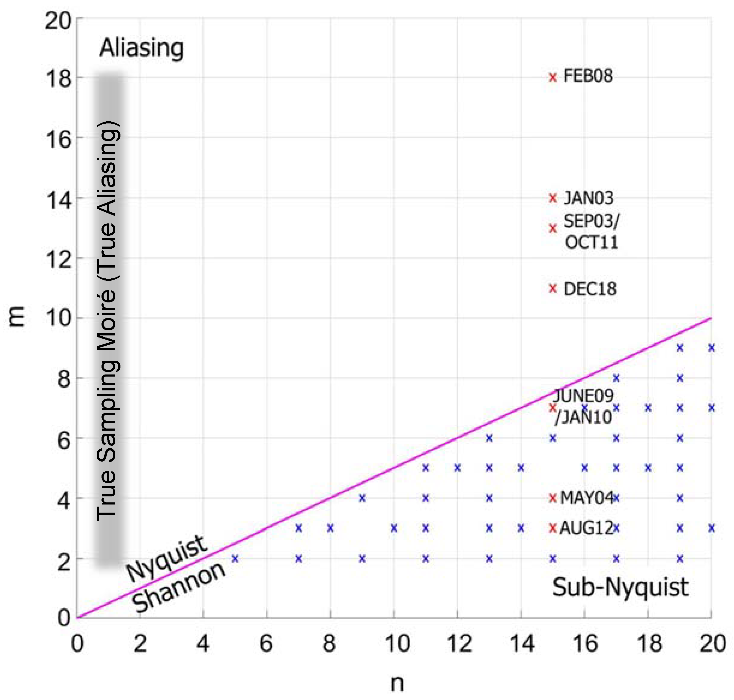
It is now expedient to examine the ratio m/n to identify all possible combinations of mutually prime integers m and n. In actuality, there are only a limited number of possible mutually prime integers, and their ratio is shown with crosses in Figure 1 (modified from [18]). The red crosses represent typical GRACE m/n ratios, but vary in time, as indicated by the dates on the graph. We will return to this graph in Section 5, where we explain how the GRACE stripes are created as sub-Nyquist artefact. The pink line in Figure 1 defines the Nyquist-Shannon border, below which the ratio m/n in Equation (1) creates sub-Nyquist artefacts from oversampling (sampling rate satisfies the Nyquist-Shannon criterion), whereas above it, the ratio m/n creates the well-known aliasing artefacts because of undersampling (Nyquist-Shannon criterion is violated). According to Williams [18], the m/n ratio that creates visible artifacts is bounded by $\frac{1}{20}<\frac{m}{n}<\frac{1}{2}$. Details on these limits are presented in Section 3.

3. A Simple Sub-Nyquist Example

What follows is a simple example of sub-Nyquist artefacts that can be created in any experiment that produces a time or data series by oversampling a quantity of interest with frequency$f_s$ near the critical neighbourhood $f_s\approx \frac{n}{m}f$ as defined by Equation (1). This example is taken from Amidror ([15]; Figure 4c) by slightly modifying the values of $f$ and $f_s$ which for the same ratio $\frac{m}{n}=\frac{1}{3}$, define $\epsilon$ that satisfies Equation (1). The reader is therefore encouraged to consult Amidror [15,16] for more details and additional examples. Although the sampling of the signal in time or space domain is a well-known process, we must emphasize that the sampling of a signal is usually taken in monotonically increasing values of time or space; this is not the case when measuring the Earth using space missions. This is an important element to consider when transitioning from the example that follows, to GRACE sampling scenarios in Section 5.

Let g(x) be a continuous periodic signal of frequency $f=2.5 \mathrm{Hz}$that is sampled with $f_s=8.25 \mathrm{Hz}$ well above the Nyquist threshold and thus, it is expected that signal g(x) will be recovered fully by the prescribed sampling. However, it so happens that $f$and $f_s$ are related through Equation (1) when m = 1, n = 3 and $\epsilon =1/4 \mathrm{Hz}$ that is, $f_s\approx \frac{n}{m}f;$ here, $\epsilon$ is sufficiently small compared to $f$. 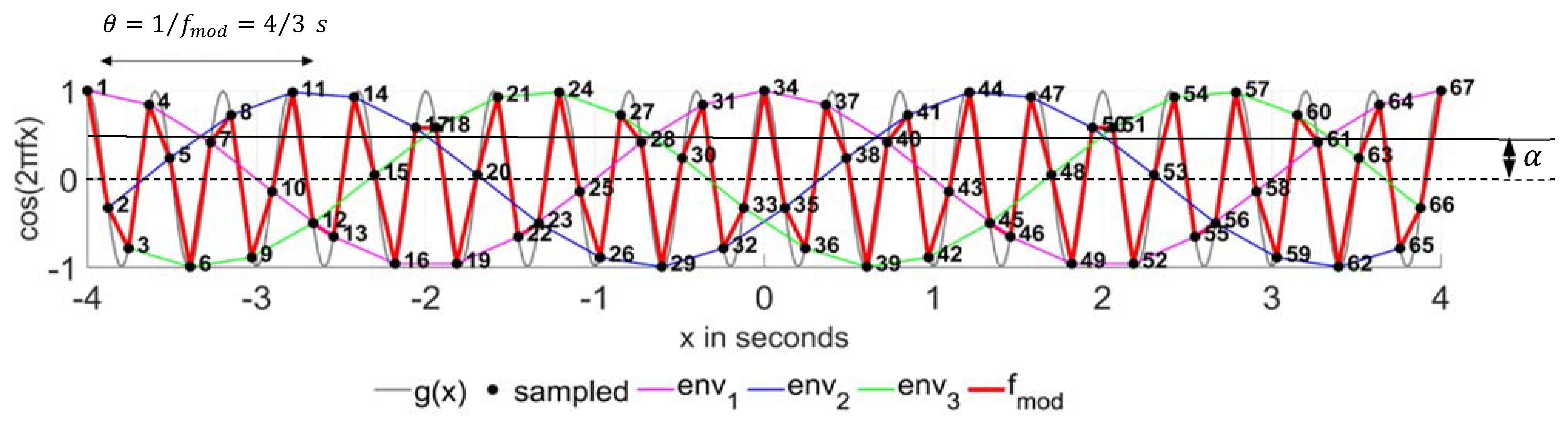The original signal g(x) (gray line) and its sampled version (red line) connecting the sample points (black dots) are illustrated in Figure 2. The sampled signal appears to be amplitude modulated by low frequency envelopes clearly visible in Figure 2. More specifically, there are n = 3 interlaced modulating envelopes, each created by connecting every third sample point (because n = 3) or we can say that successive sample points fall alternately onto the interlaced envelopes that is, for n = 3, the 1st, 4th, 7th, … sample points fall onto the first envelope, the 2nd, 5th, 8th, … points fall onto the second envelope, and the 3rd, 6th, 9th, etc. points jump onto the third envelope (cf., Figure 2).

Based on Amidror’s Theorem 5, [15] for the above example, each modulating envelope has a low frequency $f_{env}=\epsilon =1/4$ Hz, and the amplitude modulation created by the three interlaced envelopes has frequency $f_{mod}=\frac{n}{m}\epsilon =3/4$ Hz, or equivalently, any two successive envelopes are simply displaced from each other by $\theta =\frac{1}{f_{mod}}=4/3$ (θ$=a$ in [15]; Theorem 5). The above values are illustrated in Figure 2. Each modulating envelope is an expanded (stretched) version of the original signal, by $\frac{f}{\epsilon }=10$ times, i.e., it is equal to $g(\frac{\epsilon }{f} x)$, since $\frac{\epsilon }{f}<1$; in Figure 2, we count 10 full waves of the original signal within one full wavelength of a modulating envelope. The number of sample points between two successive modulating crests or valleys (on the modulated signal) is $m\times n=3$, as the reader may verify from Figure 2. We also note that because n is odd number, there is no symmetry in the modulating envelopes with respect to any horizontal axis: the crests of the positive ripples are coincident with the valleys of the negative ripples (e.g., Figure 2; at x = 0).

Furthermore, following Williams [18], the artifact (modulated signal) introduces a distortion of the original high frequency signal by $\alpha =\cos \left(\pi \frac{m}{n}\right)=0.5$ or modulation index 50 percent. The modulation index expression is derivable from the maximum phase difference between two consecutive envelopes and details can be found in ([18], Section 4.1). More generally, the modulation index is the ratio of the amount of modulation (distortion) of the carrier wave amplitude over its unmodulated amplitude. In the sub-Nyquist case, it is the magnitude of the signal in the valley of the notch divided by the amplitude of the unmodulated carrier wave (in our example it is equal to unity) ([16], Remark 2). The (normalized) distortion error due to modulation is then $ϵ=1-\alpha =1-\cos \left(\pi \frac{m}{n}\right).$ m = p e a k v a l u e o f m (t) A = M A {\displaystyle m={\frac {\mathrm {peak\ value\ of\ } m(t)}{A}}={\frac {M}{A}}}.

As noted in the previous section, the m/n ratio that creates visible artifacts is bounded by $\frac{1}{20}<\frac{m}{n}<\frac{1}{2}$. The upper limit of m/n is clearly the Nyquist (distortion $ϵ=100\%$). The lower limit namely, 1/20 stems from the requirement of a distortion level of 1 percent that is insignificant in most applications; indeed $ϵ=1-\cos \left(\pi \frac{1}{20}\right)=1.2$ percent. The larger the n (and hence the number of interlaced envelopes), the less visible and less distinguishable the envelopes become (they are very close to one another because $\theta =1/f_{mod}=m/n\epsilon$), leading to smaller and thus negligible distortion (artifacts begin to vanish). Consequently, when a signal is significantly oversampled, even when the sampling frequency satisfies the sub-Nyquist condition (cf., Equation (1)), the artifacts will be substantially reduced. More discussion on these bounds can be found in Amidror ([16]; Remark 4).

4. GRACE Latitudinal Sampling Mode and the Lorentz Reciprocity Theorem

The typical sub-Nyquist example presented in Section 3, and other various cases shown in [15] have one common characteristic: The independent variable x (space or time) of signal g(x) is monotonically increasing, forming, by definition, a series or a sequence, an approach that is not followed when sampling the Earth’s gravitational (or other field) using space missions. This is a subtle but critical point we must address before we apply the concept of sub-Nyquist artefacts to explain the striping effect on GRACE and other missions, past, present, or future.

Every Earth observing space mission involves an orbiting satellite or a constellation of satellites that take repeatedly measurements of a physical quantity (e.g., gravitational field) as the Earth spins below it. The sample measurements are taken at different locations and times following a specific pattern that does not produce a series of measurements with monotonically increasing space variable x. Take for instance GRACE, which with its nearly polar orbit, has the characteristic of sampling the Earth’s gravitational signal along the east-west (latitudinal) direction repeatedly, at the intersection of the ground tracks with the parallels (sampling points) that do not monotonically increase in space due to the spin of the Earth. The ground tracks constantly interlace in space, nearly repeating themselves (nearly repeat orbits) in about seven days.

The question now arises as to how we can apply the sub-Nyquist theory to GRACE and other Earth observing systems as it was done in [7]. In the sub-Nyquist theory, the true signal g(x) of frequency $f$ is oversampled at monotonically increasing x (non-interlaced samples) with a critical sampling frequency $f_s\approx \frac{n}{m}f-\epsilon$ ($\epsilon :$ arbitrarily chosen low frequency; not a true signal), which creates a false sub-Nyquist artefact of frequency $f_{mod}=\frac{n}{m}\epsilon$ due to n interlaced modulating envelopes. On the contrary, GRACE oversamples latitudinally, and in an interlaced mode (x not increasing monotonically), a true gravitational signal g(x) (disturbing potential) of low frequency $\epsilon$, creating a false non-interlaced high frequency signal modulated by n interlaced envelopes, each of which is a stretched version of the true gravitational signal of low frequency $\epsilon$. The above is summarized in the following

Table 1. Relationship between classical sub-Nyquist theory and GRACE signals.

Signal or Artefact	Sub-Nyquist Theory	GRACE
Signal g(x)	True Signalg(x) of high frequancy $f\gg \epsilon$ Arbitrarily small frequency $\epsilon$ so that $f\approx \frac{m}{n}{f}_s$ Non-interlaced oversampled signal $g\left(x_k\right)$	True Signal g(x) of low frequency ε (low frequency latitudinal gravitational signal) Interlaced oversampled signal $g\left(x_k\right)$
Sub-Nyquist Artefact	False Signal: Interlaced modulating envelopes of frequency $f_{mod}=\frac{n}{m} \epsilon$	False Signal: Non-Interlaced and modulated high frequency $f\gg \frac{n}{m} \epsilon$ artefact (stripes)

.

From Table 1, it is evident that in GRACE we can apply the sub-Nyquist theory (cf. Equation (1)) to the sampled gravitational signal, if and only if we deinterlace (unravel) the orbits in space, meaning that the space variable x will be monotonically increasing. After all, deinterlacing of the measurements is done during the space or time integration of GRACE orbits to develop the geopotential models.

Deinterlacing the true gravitational signal g(x) of low spatial frequency, produces a false high frequency signal $f\gg \frac{n}{m}\epsilon$ (sub-Nyquist artefact), which means that we can apply Equation (1) by interchanging the frequencies ε and $f$ of the true (sampled) signal $g\left(x_k\right)$and of the false signal (artefact), respectively to satisfy Equation (1). This, in fact implies reciprocity of the two signals that is possible according to the Lorentz reciprocity theorem in its conceptual form. In plain words, the Lorentz reciprocity theorem refers to wave phenomena, be it optics, sound, or electromagnetism, stating that the source and effect of a disturbance or a phenomenon can be interchanged. Therefore, in Equation (1), the waves with frequencies $f$ and $\epsilon$ can be interchanged, allowing us to use this equation to mean that a true low frequency modulating envelope (latitudinal disturbing potential) sampled with frequency $f_s$ can produce the false sub-Nyquist artefact of stripes of high frequency $f$. What follows is a simple example of GRACE sampling mode that demonstrates the reciprocity concept.

5. Sub-Nyquist Artefacts and the GRACE Sampled Signal

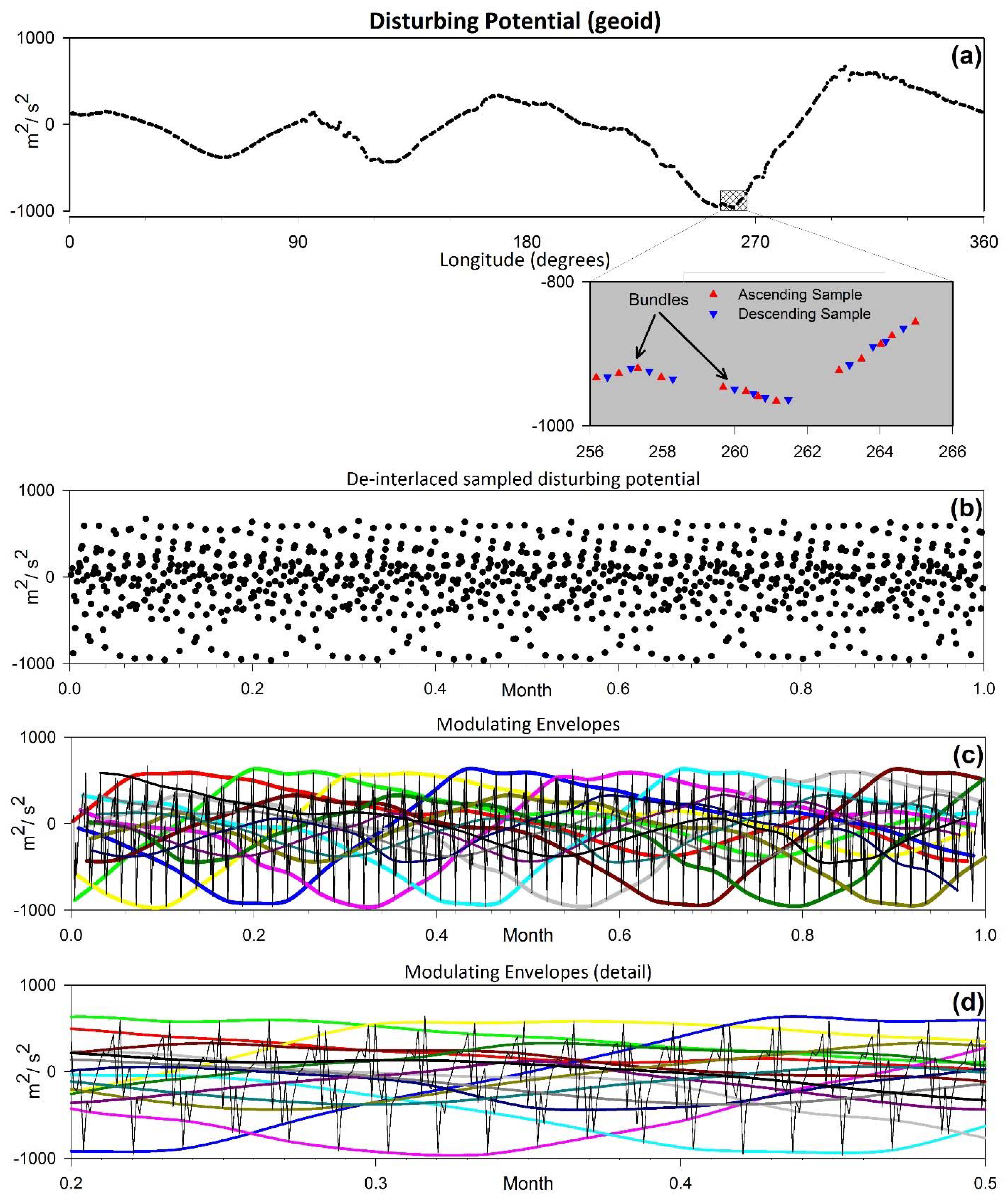
We select a random latitudinal profile of the disturbing potential (geoid), i.e., at $\varphi ={10}^{°}\mathrm{N}$, and we produce GRACE-A ground tracks during the randomly selected month of June 2009 using daily GPS precise science orbits with rate of 60 s (GNV1B files) and we classify the tracks into ascending and descending. We keep only the points (samples) at the intersection of the ground tracks with the latitude of interest $\varphi ={10}^{°}\pm {0.1}^{°}$. In Figure 3a, we show how the low degree disturbing potential (geoid) is sampled along the latitudinal profile $\varphi ={10}^{°}\mathrm{N}$. The disturbing potential is depicted with red and blue triangles signifying the ascending and descending track samples, respectively, whereas the ‘bundling’ of the ground tracks is evident, comprising, by and large, eight samples (four ascending plus four descending) and occasionally seven or nine samples. We also note that the sample points are not equally spaced thus, sampling aliasing is minimized or eliminated [17,19]. This study is carried out for nearly 30 days comprising 920 interlaced sample points from 460 orbits (cf., Figure 3a).

Subsequently, we deinterlace the sampled signal by unravelling the sample points sequentially in space as function of monotonically increasing longitude (see Figure 3b). The x-axis of Figure 3b shows the full length of the monthly deinterlaced sampled signal comprising about $429$full cycles of ${360}^{°}$ thus extending to a total length of $429\times {360}^{°}=154,{440}^{°}$ in longitude. Throughout this study, and for easier interpretation of the spectral analyses of the deinterlaced signal, the x-axis is normalized by the total length of the signal therefore the graphs extend for one month. Equivalently, we could rearrange the sample points with respect to increasing time. Sample points on the ascending and descending nodes are shown in red and blue, respectively.

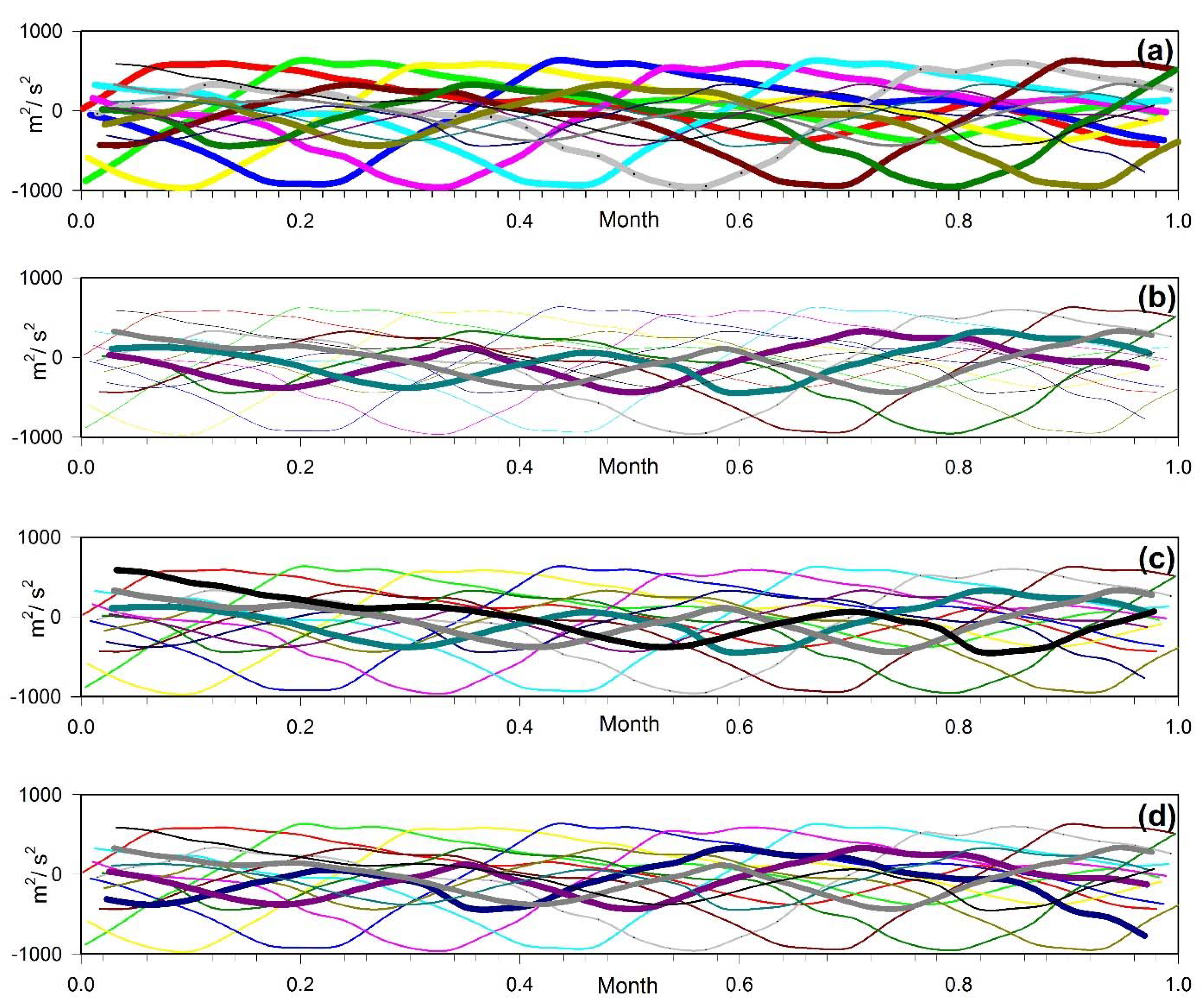
In Figure 3b, we easily observe that the sample points show a specific wavy pattern that looks like a set of interlaced low frequency modulating envelopes. We further realize that if we choose an arbitrary sample point and connect it with the next 15th point and so on, a low frequency modulating sine-like wave is created. Using all sample points, 15 such interlacing sine-like waves are created in total. That is, the 1st, 16th, 31st, … sample points fall onto the first envelope, the 2nd, 17th, 32nd, … points fall onto the second envelope, and so on (Figure 3c). Due to the quasi-periodic character of the disturbing potential and unequal sample spacing, we do not expect perfect modulating sine waves or constant distortion levels along a latitudinal profile as in the example (vis., Figure 2). After all, each envelope is expected to be the expanded version of the original signal, namely the disturbing potential profile (Figure 3a). We note that Amidror’s Theorems 5 and 6 [15], although developed on the assumption of sampling a periodic function g(x), they can be applied when function g(x) is quasi-periodic but still contains a strong periodic component, as is the case with the latitudinal characteristics of the geoid.

To understand the structure of the deinterlaced signal and the modulating envelopes and how this generates the sub-Nyquist artifact of stripes, we perform several simple calculations as in the example of Section 3. Due to the quasi-periodic nature of the disturbing potential, the unequal sampling interval and its highly variable magnitude, the results of our calculations express average values:

(a)

Using the deinterlaced sample we calculate that in June 2009, GRACE had a near-repeat orbit at $R/D=107/7$, (or $R/D=\beta /\alpha$ according to [20]) i.e., the repeat orbits occurred after 107 revolutions in seven days [21]. In our calculations, ‘near’ means less than 0.8° separation in longitude of repeat orbits. Clearly the ratio $\frac{107}{7}\approx 15.3$ shows the number of orbits per day. It is important to link these ratios to the resonant theory of orbits [20,21,22] by showing $R\approx nm$ and $D=m$.

(b)

As discussed in [7], we set m = 7 (number of days required to have a nearly repeat orbit) and n = 15 (number of complete orbits in one day). In space domain, the magnitude of sub-Nyquist artifacts peak n times across the globe and within consecutive peaks there are m oscillating waves (stripes). Note that m changes over time (see Figure 1) while n remains constant throughout GRACE mission.

(c)

The number of sample points between two successive modulating crests or valleys (on the modulated signal) is $m\times n=105$. On average, we count $107$ points (Figure 3c).

(d)

The number of times the disturbing potential is re-sampled in a month (in the deinterlaced mode) is 429. Therefore, its frequency is $f=429$ CPM (cycles per month).

(e)

The phase shift of a modulating envelope with respect to the adjacent one, i.e., the normalized distance between two adjacent crests (cf., Figure 3c,d) is estimated to be $\theta =0.116$ months or $f_{mod}=1/\theta =8.6$ CPM. This is illustrated in Figure 3c, where 8.6 modulating crests span the entire month.

(f)

The ratio of the number of samples to the number of modulations i.e., $919/8.6\approx 107$ is equal to the number of bundles we count in the profile (Figure 3a) and equal to the number of orbits it takes to have a repeat orbit.

(g)

From $f_{mod}=\frac{n}{m}\epsilon$, we calculate the low frequency of the modulating envelope $f_{env}=\epsilon =4.01$CPM. As expected, $\epsilon \ll f.$

(h)

The latitudinal spacing of the ground tracks is unequal and the samples are bundled in groups of eight (four ascending and four descending) or occasionally in groups of seven or nine (Figure 3a). The effective sampling rate calculated from Equation (1) using $f=429$ CPM and $\epsilon =4.01$CPM is $f_s^{eff}\approx 928$ samples per month, which gives $f_s^{eff}>2f$ and thus satisfies the Nyquist-Shannon condition. Given the unequal sampling interval, we do not expect any aliasing artifacts.

(i)

Because n = 15 is odd number, there is no symmetry in the modulating envelopes with respect to the horizontal axis. This is clear from Figure 3 and Figure 4.

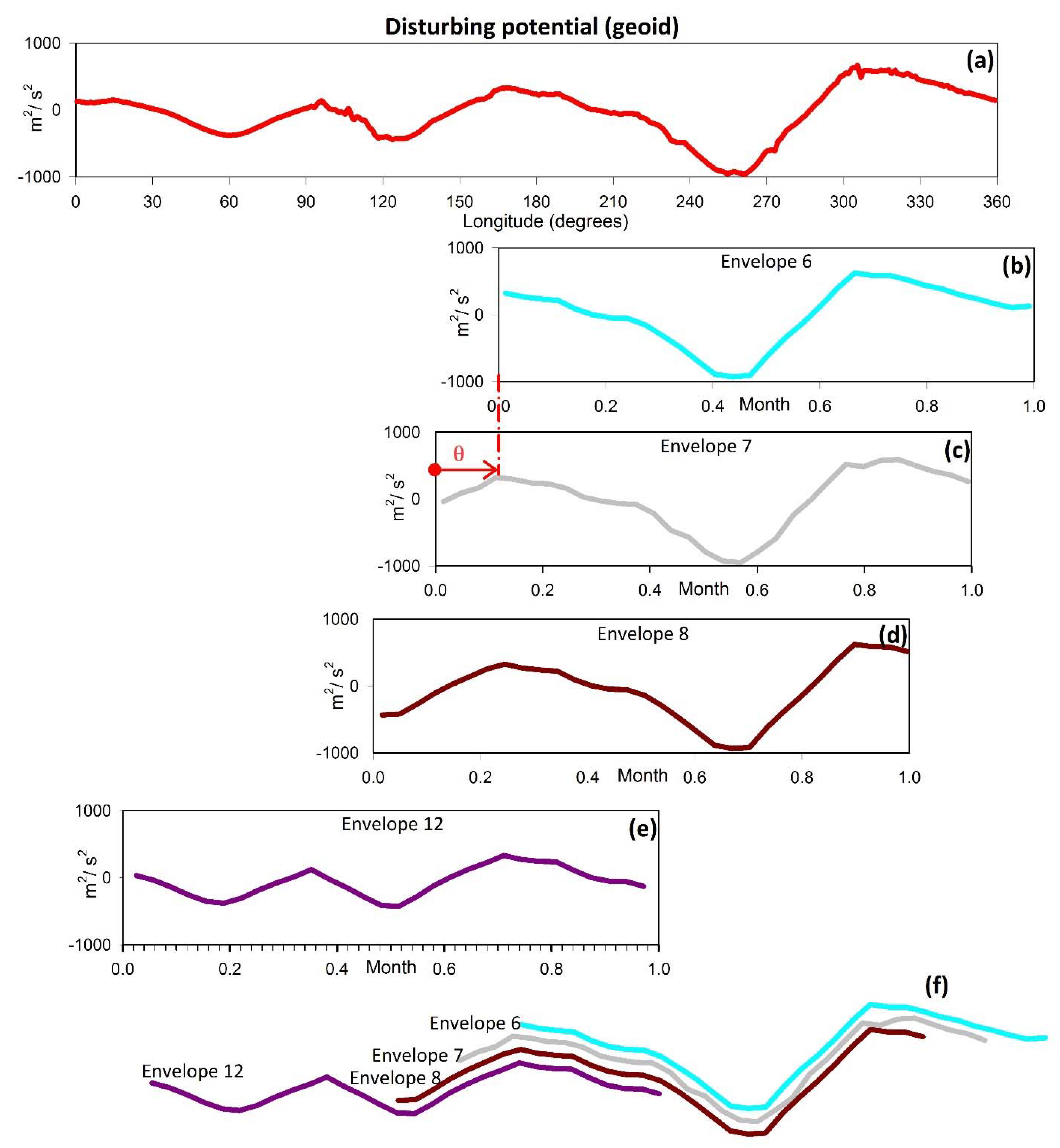
(j)

Each modulating envelope is the expanded (stretched) version of the disturbing potential by $f/\epsilon =107$ times. In Figure 5, we illustrate this property by juxtaposing the disturbing potential with a random selection of envelopes after contracting them back to the disturbing potential scale.

(k)

In Figure 4 we observe that there are visible, smaller less-clearly defined amplitude modulations within the all-encompassing modulating envelopes, though all of them have the same low frequency and the same phase offset$\theta =0.116$ between adjacent ones (Figure 5). The lower intensity modulation is due to the low amplitude segment of the disturbing potential.

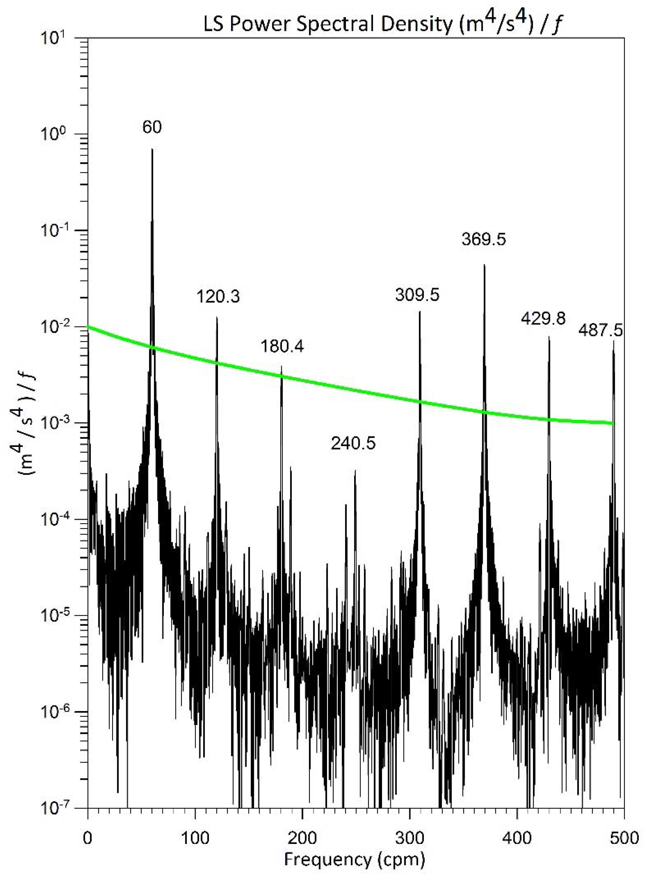
Contrary to the example in Section 3, where we have pure sine modulating waves (envelopes) of the same amplitude creating a uniform sub-Nyquist artifact, here we have a modulating signal, namely the disturbing potential that is quasi-periodic of varying amplitude. Because the signal is not perfect or even nearly perfect sinusoid, albeit showing a systematic structure, it is expected that in the frequency domain, it will show many harmonics of the fundamental frequency $f_0=60$CPM (there are 60 dominant wavelengths in Figure 3c). Indeed, the least squares power spectral density [23,24] of the deinterlaced signal shown in Figure 6 verifies that the modulating frequency $f_{mod}=8.6$ CPM is absent, as it should. There are seven very distinct and nearly perfect harmonics of $f_0=60$CPM in the spectrum. The frequency of the 6th harmonic is nearly identical to the frequency of the false signal in the de-interlaced sample namely, $f=429$ CPM (see point (d) above).

Lastly, we note the intriguing relationship $f_0/m=60/7=8.6=f_{mod}$, and consequently $f_0/n=60/15=4=\epsilon$. The above are in full agreement with the GRACE resonant orbit theory [20]. In the next section, we discuss the values of the ratio $R/D$ vis-à-vis the intensity of stripes.

The strongest harmonic $f_0=60$ CPM is the frequency of the carrier wave modulated by the interlaced envelopes. In cases of perfect sine signals, the modulating envelopes are perfect sine waves of low frequency and the artifacts (modulations) create regular wave patterns of constant frequency and uniform modulation distortion (cf., Figure 2). In our case, the modulating envelopes are stretched replicas of the latitudinal profile of the low frequency disturbing potential that is not a perfect sine wave as illustrated in Figure 3, Figure 4 and Figure 5 and thus the modulating envelopes will be irregular introducing variable distortion levels which cannot be calculated by the modulation index formula discussed in Section 3.

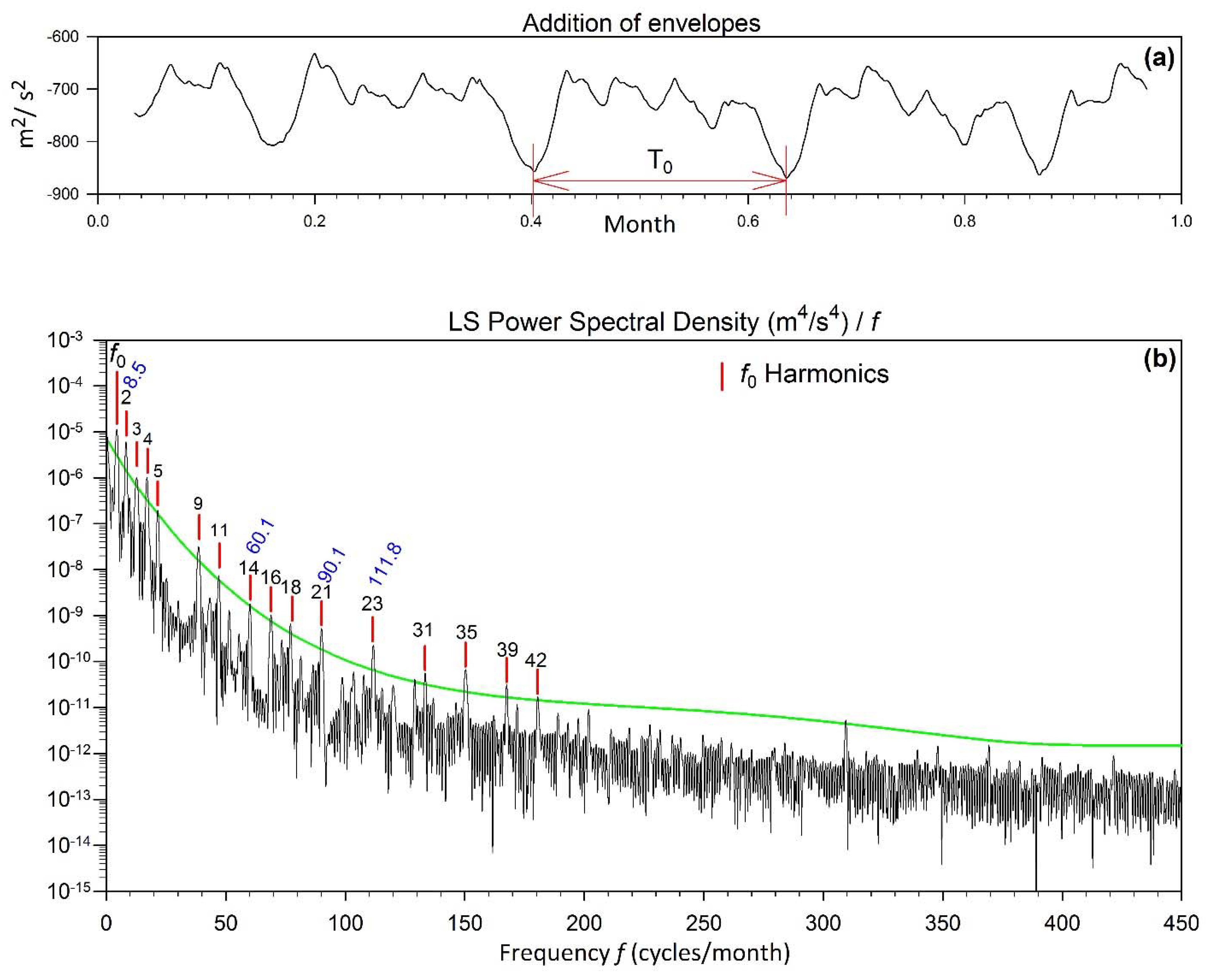
Since the sub-Nyquist (pseudo-moiré) artifacts are the modulations of the carrier wave [25] then, the stripes are the result of the combined (beating) effect of all the modulating waves. Therefore, we superpose all 15 envelopes (additive mode) and create a new data series for the entire month shown in Figure 7a. The superposition is clearly not a sine wave, and we expect that the power of the fundamental frequency $f_0=1/T_0$ will spill-over to several harmonics in the frequency domain. The beating of the 15 envelopes shows the total sub-Nyquist artifact (stripes) which appears to be a few percent of the disturbing potential with a fundamental frequency of $f_0=4.3$CPM. Figure 7b displays the least squares power spectral density showing, among others, the modulating frequency $f_{mod}=8.5$ CPM and the fundamental frequency of 60 CPM of the false deinterlaced sampled disturbing potential.

In our previous work [7], we performed a lengthy analysis of stripes from 36 monthly latitudinal profiles at $\varphi =+{30}^{°},$ using GRACE RL04 and RL05 level 2 data (d/o = 120 and d/o = 96, respectively). We concluded that there was an important near time-invariant similarity of their spectra both in the individual monthly profiles and in the entire 36-month profile. We noted that there were three consistent spectral peaks at 63.5, 76.7 and 79.4 cycles per 360° longitude. Importantly, the longitudinal profiles showed a modulated pattern in the space domain ([7]; Figure S1), like the one we see in this study. Clearly, since the modulation is induced by the quasi-periodic disturbing potential profile, the modulation pattern is different at different latitudinal profiles as is along the same profile thus explaining why the stripes in the GRACE models are of varying intensity across the globe. The frequencies found in this analysis are close to the ones obtained from RL04 but at latitude +30°. This is because the latitudinal structure of the low frequency disturbing potential is nearly consistent globally as pointed out by Peidou [26] and Peidou and Pagiatakis [7].

The intriguing structure of the latitudinally sampled disturbing potential resulting in the longitudinal structure of stripes, has the following characteristics:

(a)

A systematic and dominant long wavelength latitudinal structure of the disturbing potential, visible in any global geoid map, of a broad sectorial structure of very low degree [7,26] with two ‘corridors’ of positive undulations: The first corridor extends from Greenland/Fennoscandia down to West Africa and between the South Atlantic and Indian ocean while the second corridor extends from Japan, down to South China Sea and Indonesia, and to Eastern Australia/South Pacific Ocean. Between the two corridors there is the major geoid low in the Indian Ocean. Similar sectorial structures of lower intensity can be seen along the Americas and the Atlantic Ocean.

(b)

A specific latitudinal sampling pattern of unequal space interval, bundling of the ground tracks, frequency of the repeat orbits, and most importantly the interlaced sampling (deinterlaced during orbit integration). The latitudinal sampling of the low frequency disturbing potential is not uniform and its effective frequency, although clearly satisfies the Nyquist-Shannon criterion, it has a specific value that supports the creation of Sub-Nyquist artifacts.

The above points provide alternatives to eliminate the sub-Nyquist artifacts at source by appropriately designing, monitoring, and adjusting the orbits of future space missions. We discuss such options in Section 7 and Section 8 of this contribution. Furthermore, to support of the above findings, we performed extensive simulations, assuming that the disturbing potential is a perfect sine wave sweeping the frequencies from 1–7 cycles per 360° longitude and sampled at the exact GRACE sampling rate. The simulations (not shown in this contribution) revealed that sub-Nyquist artifacts are created only when the disturbing potential is in the narrow band of 2–5 cycles per 360° longitude. This confirms that the low frequency latitudinal disturbing potential structure combined with the latitudinal sampling characteristics imposed by the orbit design, create the artifact of stripes. As noted in [7], other similar mission designs, such as CHAMP and Swarm also show sub-Nyquist artifacts.

6. GRACE Sampling Characteristics and Sampling Artefacts

The unconstrained GRACE spherical harmonic solutions of any release (RL01–RL06) are susceptible to the artefact of stripes [27]. Because of the presence of the of stripes in the measurements (sampled signal), the spherical harmonics that are estimated by least-squares, are contaminated from these false signals especially in the higher spectral degrees. Of note is that other techniques used to represent the Earth’s gravity field, such as mascons [28,29] perform better in terms of reducing the stripes in the first place (before a-priori filtering) as they avoid the harmonicity of the solution and therefore limit the propagation of the artefact in the higher harmonics. We analyze the GRACE orbits to ascertain that their geometry is spatiotemporally non-stationary, and this non-stationarity is expressed through the variability of index m. We make a direct link between the nodal revolution period $R$ and the (synodic) days D it takes to have repeat orbits [21] with indices $m$and $n$ thus relating the sub-Nyquist artifacts with the resonant orbits.

To fully capture how the various sampling parameters impact the stripes shown in the final models, we analyze the patterns of ground tracks of various months using the daily precise orbit solutions of GRACE and GRACE-FO in a time span of 15 years. While the number of envelopes $n$ remains fixed to 15, $m$ changes in the interval [3,18]. Considering the Nyquist-Shannon criterion, sub-Nyquist artefacts occur only when $2m\le n$. If this inequality is not satisfied, then the artefacts present in the reconstructed signal become sampling moiré (aliasing) effects, yet at critical m/n ratios. We note here that these sampling moiré effects, are not the same as the striations encountered in GRACE literature as they are not driven from the well-known aliasing sources (tides, atmosphere, and continental water mass).

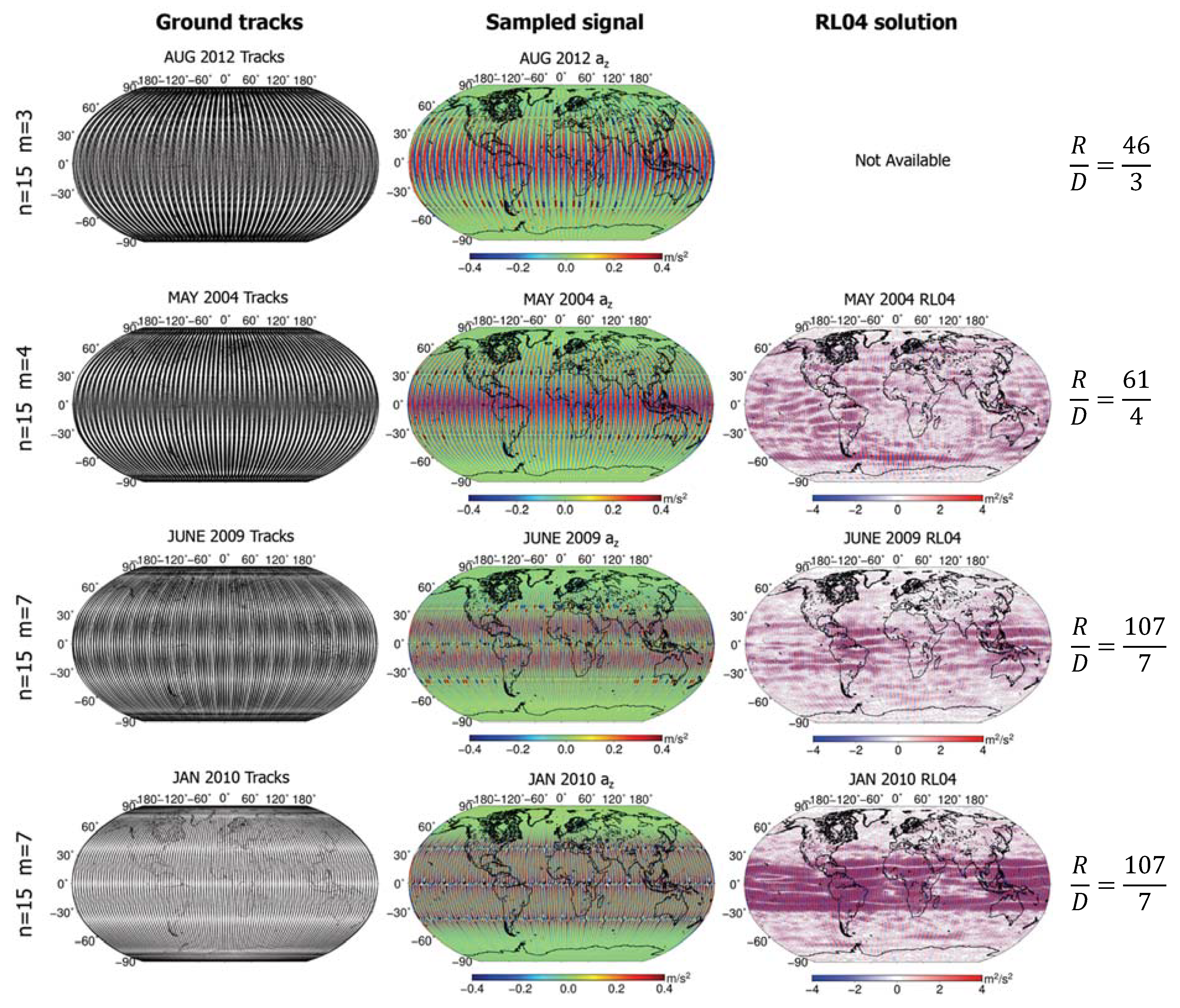
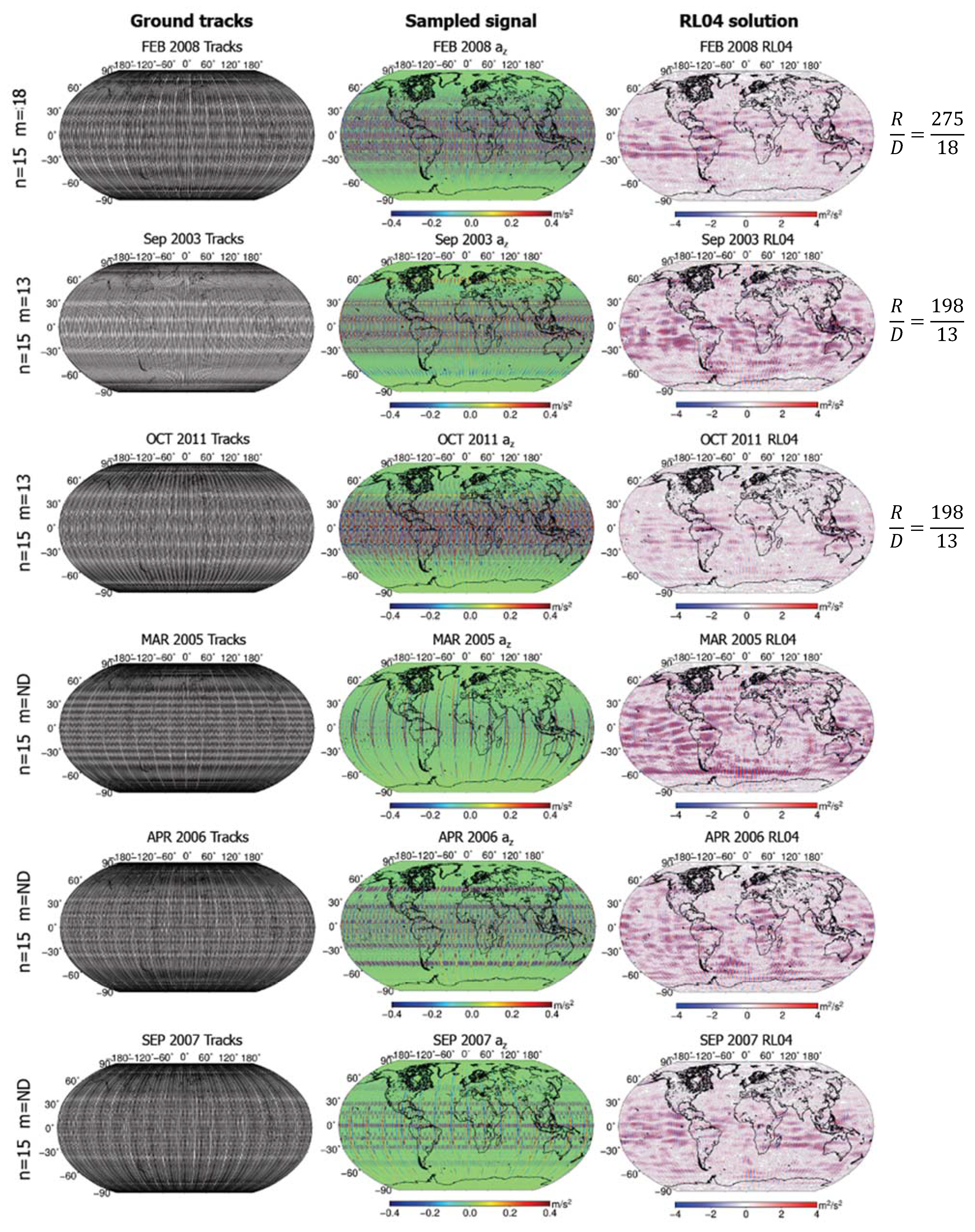
To fully understand how the geometry of the orbits induces stripes in the sampled signal and how the stripes of a specific geometry relate to the resonant orbits, we analyze 10 random months between 2003 and 2018. Between 2003–2012 we use GRACE GNV1B daily files and for 2018 we use GRACE-FO GNV1B daily files. For each month analyzed (vis. Figure 8 and Figure 9) we use:

(a)

The ground tracks (left panels).

(b)

The sampled total accelerations, (middle panels): We calculate the time derivative of the spacecraft velocity to estimate the total acceleration (gravitational plus non-gravitational) along each axis of the ITRF to show that stripe-like structures are present in the raw observations that are used to develop the GGMs. Consequently, we take the acceleration differences between the leading and the trailing satellites. In this study we display only the acceleration differences along the z-axis for visualization purposes since they are more pronounced than in the other axes. The reader can find all three acceleration differences in ([7], Figure 1) and in [26].

(c)

The gravitational potential derived from RL04 solutions (right panels): We calculate the gravitational potential for all monthly solutions, using RL04 spherical harmonics (up to 120 degree and order) and then we subtract the mean field to accentuate the structure of stripes. Note that RL04 solutions are used due to the increased magnitude of stripes evident in the d/o = 120 solutions.

Figure 8 and Figure 9 show various GRACE monthly solutions, where the orbits exhibit different combinations of $m$ and $n$. The solutions are sorted in ascending order with respect to integer $m.$ The number of bundled orbits varies from month to month and is close to $R$. Interestingly, there are a few months between 2005–2007 in which the interlacing pattern is not very well defined. That is, the interlacing of the orbits is not fixed in time because integer $m$ varies within the month.

The stripes evident in the sampled signal (e.g., in $a_z$) are created along the orbit and therefore they demonstrate very similar latitudinal spectral characteristics with the ground tracks. It seems that the most affected regions in the sampled signal are the ones between $-{60}^{°}\le \varphi \le {60}^{°}$. Since index n is constant for GRACE (n = 15), it is m that is critical in the generation of the stripes. Months with variable $m$ result in stripes of lower magnitude. In addition, when the ratio m/n does not form critical ratios outside the sub-Nyquist region and is away from the ‘true sampling moiré’ region (cf., Figure 1; shaded region) it is expected that the magnitude of the stripes and perhaps any residual striations that are produced by the low frequency phenomena of tides, atmosphere, and continental water mass will significantly be reduced or perhaps eliminated.

The RL04 solutions truncated to the nominal spectral degree of GRACE orbits (i.e., $l_{max}\le 120$), demonstrate nearly identical peak frequencies among all the analyzed months, exhibiting different frequencies with respect to the latitudinal profiles (they range between 90–110 $\mathrm{c}/\ell$ along various latitudes).

The stripes in the sampled signal during paired months (months with the same set of $m$ and$n$) have different magnitudes, although their spectral characteristics are the same (e.g., 3 September and 11 October; 9 June and 10 January). Although in the time domain the number of days required for a ground track to cluster in a bundle (track interlacing) is the same, the distance between the tracks that form a bundle (therefore the width of the bundle) is not fixed in space domain, a behavior that impacts only the magnitude of the stripes and not their frequency (e.g., Figure 8; rows 3 and 4). Additionally, RL04 solutions are the summation of all the three stripy sources, mentioned above (i.e., errors along the track, aliasing, and sub-Nyquist) and therefore we expect a variation in their magnitude.

With regards to the magnitude of stripes coming purely from oversampling the disturbing potential at a critical frequency (sub-Nyquist region), the variation of the magnitude of the artefact is well explained by the theory of modulation; if the ground tracks resemble a carrier wave superposed on the low-frequency disturbing potential, and the highest the density of tracks in the bundled tracks, the strongest the modulation and therefore the highest the magnitude of the stripes ([26], Section 5.4). A good discussion on the impact of the density of the repeat orbits in the accuracy of GRACE models can be found in [20,30].

Our analysis hints that the sub-Nyquist artifacts (stripes) are related to the resonant orbits as studied by Klokočník et al., [20,31]. Naturally, every space mission exhibits resonance, but the longer it takes to be established, the better it is from the perspective of the stability of measurements and solutions, and the stripes will exhibit lower intensity.

It is clear from the above that the sub-Nyquist ratio m/n is directly related to the resonant conditions of GRACE having m equal to the number of days it takes to have a nearly repeat orbit. Therefore, m is the key variable that defines the resonances of the orbits. Figure 8 and Figure 9 above are very revealing in establishing the variability of m over the GRACE mission life. When the ratio m/n satisfies the condition $\frac{1}{20}<\frac{m}{n}<\frac{1}{2}$ [18] it produces bundled ground tracks (first column) and strong stripe patterns in the geopotential models (Figure 8; third column).

Figure 9 shows characteristic cases in which m is either not well defined (varies significantly in a month) or when defined, m/n violates $\frac{1}{20}<\frac{m}{n}<\frac{1}{2}$. Despite the ratio m/n being in the ‘sampling moiré’ region (Figure 1), it is away from the “pure sampling moiré’ region, while forming critical ratios of mutually prime integers, even in the case $\frac{m}{n}=\frac{18}{15}=\frac{6}{5}$ (February 2008). Figure 9 shows R/D ratios calculated in this study according to [31] and agree with the values posted in ([20], Figure 6). In such cases we observe no systematic stripe structures, or the regional stripes are weak. The example we presented in this study (Section 5) had a clear resonant structure at 107/7 (border line sub-Nyquist artifact).

7. Eliminating the Stripes: An Open Question

Although the analyses presented in Section 5 and Section 6 demonstrate in detail how the sampling characteristics of GRACE create stripes in Level 1B data, the presence of the artefact in the gravity field models still poses limitations in the recovery of geophysical signals of finer spatial scales (e.g., smaller than 200 km). Traditionally, filtering schemes are employed to minimize the magnitude of stripes, with the trade-off of geophysical information loss. Our analyses suggest that the artifact contaminates the signal while it is sampled, making elimination at source challenging. We tried to break the sampling pattern in a post-processing analysis by randomly removing sample points, but the magnitude of stripes appeared to attenuate only after a harsh cut-off of 50 percent of the sample points. Therefore, the main recommendation that can be made to eliminate stripes refers to a cautious design of orbits of new missions.

Newly designed orbits should avoid the critical sampling rate $f_s$ defined by Equation (1) as function of the disturbing potential latitudinal frequency $f\in \left[1.5, 3.1\right]$ cycles per 360° longitude, as shown in [7]. It appears that when the ratio $m/n$ is within the sub-Nyquist region the stripes are greatly pronounced, particularly when resonances of low ratio are present. Furthermore, reduction of the sub-Nyquist artifacts at source may be achieved by appropriately monitoring and adjusting the orbits of future space missions to avoid harsh resonances (short-repeat orbits) that amplify the magnitude of stripes. The latter was also suggested by Wagner et al. [21] to maneuver the GRACE pair (high or low) to avoid short repeat cycles that cause reduced precision or loss of information in future monthly GRACE gravitational field models. When the ratio $m/n$ jumps into the sampling moiré region while being critical (m and n are mutually prime integers), the stripes are less structured and of lower magnitude. Even in sampling moiré region, critical $m/n$ ratios must also be avoided in future missions. Extensive simulations should be performed to achieve m/n ratios from critical values.

8. Conclusions and Discussion

Our study focused on the sub-Nyquist artefacts that are present in the gravity products of GRACE and GRACE-FO missions in the form of longitudinal stripes. Simple examples and real GRACE Level-1B data were employed to demonstrate in detail how the artifacts appear in the measurements, during the sampling process. The sample measurements are taken at different locations and times following a specific pattern that produces a series of measurements that is not monotonically increasing in space and is interlacing (bundling) in the same region every m days. A low degree gravitational signal, the disturbing potential, while sampled with this specific pattern drives envelopes that modulate the sample signal in the east-west (latitudinal) direction. The result of this modulation is a false highly oscillating wave, which is in fact the well-known artefact of stripes. Additionally, analysis of GRACE Level-1B and Level-2 data over a wide timespan quantified the variability in the orbital characteristics of the mission and showed how they affect the characteristics of the stripes shown in the sample signal and the Level 2 models.

We attempted to reduce or eliminate the stripes by deconstructing the sub-Nyquist pattern via an elimination of sample points thus, altering the effective latitudinal sampling characteristics of the mission or, by extension, varying the orbital characteristics through integers m and n that characterize the sampling pattern and the orbit resonance. However, the gravity signal retrieved from GRACE is contaminated by the artifacts during the sampling process, and therefore minimization of stripes at source could not be achieved by this approach. Finally, to minimize the presence of stripes in Level-2 data products, it is recommended that orbits of future missions should be designed to avoid the critical m/n ratios as shown in Figure 1, that also relate to critical resonant orbits, or if impossible, at least m/n should approach the lower limit in the sub-Nyquist region $\frac{1}{20}<\frac{m}{n}<\frac{1}{2}$. For completed missions, or missions that are already active, force modelling the latitudinal disturbing potential may be a viable and most preferred approach to filtering.