Spectral-Spatial Offset Graph Convolutional Networks for Hyperspectral Image Classification

Abstract

In hyperspectral image (HSI) classification, convolutional neural networks (CNN) have been attracting increasing attention because of their ability to represent spectral-spatial features. Nevertheless, the conventional CNN models perform convolution operation on regular-grid image regions with a fixed kernel size and as a result, they neglect the inherent relation between HSI data. In recent years, graph convolutional networks (GCN) used for data representation in a non-Euclidean space, have been successfully applied to HSI classification. However, conventional GCN methods suffer from a huge computational cost since they construct the adjacency matrix between all HSI pixels, and they ignore the local spatial context information of hyperspectral images. To alleviate these shortcomings, we propose a novel method termed spectral-spatial offset graph convolutional networks (SSOGCN). Different from the usually used GCN models that compute the adjacency matrix between all pixels, we construct an adjacency matrix only using pixels within a patch, which contains rich local spatial context information, while reducing the computation cost and memory consumption of the adjacency matrix. Moreover, to emphasize important local spatial information, an offset graph convolution module is proposed to extract more robust features and improve the classification performance. Comprehensive experiments are carried out on three representative benchmark data sets, and the experimental results effectively certify that the proposed SSOGCN method has more advantages than the recent state-of-the-art (SOTA) methods.

1. Introduction

In recent years, hyperspectral imaging technology has witnessed rapid and sustained development, and the corresponding spectral resolution and spatial resolution have been significantly improved, which is beneficial to the accurate classification and recognition of surface objects [1]. HSI classification has gained wide attention in various domains, including environmental monitoring, disaster prevention and control and mineral deposit identification [2,3,4,5]. However, due to the large amounts of spectral bands, HSI classification tasks still suffer from many challenges. The most remarkable challenge is the Hughes phenomenon, in addition to high information redundancy and high computational cost. Feature extraction is one of the effective ways to solve these problems. However, complications situations such as spectral variability [6] bring a great challenge to the feature extraction task.

In the face of these situations, spatial context is fused to obtain discriminating spectral-spatial features such as morphological profiles (MPs) [7], attribute profiles (APs) [8] and Markov random fields (MRFs) [9] which use hand-crafted features and therefore require considerable expert experience. Recently, deep learning has shown its potential in mining spectral-spatial features of HSI. For instance, recurrent neural network (RNN) [10] and generative adversarial networks (GAN) [11]. In particular, convolutional neural networks (CNN) are widely used to extract robust spectral-spatial features for HSI classification tasks. For example, Zhang et al. [12] designed a separate dual-channel CNN model which can automatically extract more robust hierarchical spectral-spatial features. Zhong et al. [13] enhanced the representation capability of CNN model through designing residual blocks to learn discriminative spectral-spatial features. However, CNN models only perform convolution operations on regular-grid image regions with fixed size of kernels, which fail in flexibly capturing various geometric structures of different local regions in HSI data, resulting in loss of class boundary information and the occurrence of misclassification.

Comparatively, a graph convolutional network (GCN) [14] can be directly applied to irregular (or non-grid) data, making full use of image features and flexibly preserving class boundary information. In [15,16,17], GCN was applied to HSI classification with relatively satisfactory results. But these tasks require a high computational cost which is particularly heavy for hyperspectral images because they compute the adjacency matrix between all pixels. Wan et al. [18] reduce the calculative cost of the adjacency matrix by super-pixel segmentation such as the simple linear iterative clustering (SLIC) [19] and regard these super-pixels as graph nodes, and then extract multi-scale spectral-spatial features by multi-scale dynamic GCN (MDGCN). However, they take a full-batch network learning approach, which leads to slow gradient descent. In addition, the classification performance of GCN model based on super-pixel segmentation is seriously affected by the result of super-pixel segmentation, and the hyperparameters in super-pixel segmentation algorithm are difficult to be determined. Different from the work in [18], Hong et al. [20] developed a minibatch graph convolutional network (miniGCN), which only needs to construct HSI subgraphs and can be trained in minibatch fashion. Nevertheless, above method models long-range spatial relations in HSI, ignoring the local spatial context information, which can more effectively alleviate the spectral variability in the HSI classification.

To address the above limitations in existing GCN-based methods and make GCN-based HSI classification algorithms can achieve better performance, we propose a simple but effective spectral-spatial offset graph convolutional network for HSI classification (termed SSOGCN) in this letter. Different from the traditional GCN-based classification methods, our proposed method only needs to construct the graph structure between the pixels in the patch, while reducing the computation cost of the adjacency matrix and memory cost. In addition, we develop the offset graph convolution (OGC) module to emphasize important local spatial information by subtraction operation, which actually acts as a filter. To be specific, we firstly input a HSI patch which contains the local spatial context information and then use the automatic graph learning (AGL) module to construct the graph structure between pixels in the patch. Next, our GCN-based network is employed to extract the hierarchical spectral-spatial features of the HSI patch and classify the patch finally. In this work, our GCN-based network can effectively capture the local spatial context correlation which traditional GCN-based classification methods ignore, and meanwhile, can be trained in minibatch fashion and speeds up the convergence speed of training.

There are six sections in this article. The Section 2 retrospectively covers some related works. The Section 3 introduces the SSOGCN method we proposed in detail. The Section 4 is the experimental results and analysis. The conclusions are presented in the Section 5.

2. Related Works

We detail the development process of graph convolutional network in Section 2.1, which are divided into graph convolutional network in spectral domain and graph convolutional network in spatial domain. In Section 2.2, we review certain representative works on HSI classification task. Besides, we analyze the status of graph convolutional network in hyperspectral image classification.

2.1. Graph Convolutional Network

With the complete development of graph convolutional network theory, graph convolutional network has been widely applied in various fields. There are some representative works such as recommendation system [21] and natural language processing [22].

Compared with CNN and RNN, graph neural network has the advantage that it can directly process graph-structured data in non-Euclidean space. Its concept was first proposed by Gori et al. [23]. Convolution on graph can be divided into two groups according to different perspectives [24]. Spectral graph convolution uses the graph Fourier transform to transform the graph signal to the spectral domain, and then carries out the convolution operation in the spectral domain. Spatial graph convolution aggregates the node features from the perspective of spatial domain.

Spectral CNN (SCNN) [25] is a representative pioneering work in spectral methods, where the graph signal is converted into spectral domain by graph Fourier transform followed by performing convolution operation in spectral domain. The convolution kernel in this work is defined as a set of learnable parameters which is relevant to Fourier bases. However, the number of parameters in Spectral CNN is closely related to sample size, and this work is based on the eigen-decomposition of Laplacian matrix which is a complicated step. Such a model has a high computational cost on large-scale graphs and is easy to overfit. Subsequently, ChebyNet [26] used Chebyshev polynomials to fit the frequency response function, where complex eigen-decomposition step is no longer be required and the number of parameters was only related to the order of the polynomial, which is much smaller than the sample size. Afterwards, Kipf and Welling [14] further optimized ChebyNet and simplified the polynomial to the first-order approximation, which provided a more efficient graph filtering operation than ChebyNet.

In spatial graph convolution, the convolution operation on each node is regarded as linear weighting within neighbor nodes, namely the weighting function, which characterizes the influence of adjacent nodes on the target node [27]. For instance, in GraphSAGE [28], random sampling among neighbor nodes is carried out first, and then aggregation functions are used to aggregate the sampled neighbor nodes. In graph attention network [29], self-attention mechanism is used to aggregate neighbor nodes. In addition, MoNet [30] deems that convolution is the superposition of multiple weighting functions on neighbor nodes, which can be regarded as a unified framework of spatial approaches.

2.2. Hyperspectral Image Classification

Feature extraction is a very important step for hyperspectral image classification. A lot of feature extraction algorithms have been successfully utilized for HSI classification [31,32,33]. Principle component analysis (PCA) [34], linear discriminant analysis (LDA) [35], locality preserving projection (LPP) [36], neighborhood preserving embedding (NPE) [37] are widely applied to HSI classification. Nevertheless, due to the complex situation such as spectral variability, it is hard to classifies various land-cover categories accurately by only utilizing spectral features. Therefore, it has become an inevitable trend to use spatial context information for the classification task of HSI. Recent spectral-spatial HSI classification methods include morphological profiles (MPs) [7], attribute profiles (APs) [8] Markov random fields (MRFs) [9], methods based on segmentation techniques [38,39], and methods based on sparse representation [40] that excavate rich spectral-spatial joint features. Nonetheless, all of these methods have poor performance on capturing subtle differences between different categories or large differences within the same category, and they heavily rely on expertise, since they employ hand-crafted spectral-spatial features.

As an advanced technology, deep learning has drawn increasing attention in various computer vision tasks [41], since it can automatically extract effective feature, thus averting the complex hand-crafted feature engineering [42]. Recently, it has also brought revolutionary changes to HSI classification task [43]. Chen et al. [44] introduced a stacked autoencoder (SAE) for HSI classification to learn hierarchical features in an unsupervised manner for the first time. Subsequently, Chen et al. [45] proposed the deep belief network (DBN) model to obtain robust features through the deep belief network and complete classification task through logistic regression. Meanwhile, Shi and Pun [10] introduced a recurrent neural network to HSI classification, which can capture the spatial dependence and excavate multiscale and hierarchical spectral-spatial features. Moreover, Zhu et al. [11] applied improved generative adversarial networks (GAN) to the HSI classification, with the input of three PCA components and random noises. There is a recent work on treating a continuous spectrum as a sequence and mining spectral features with Transformers which are good at processing sequence data [46]. CNN, in particular, has shown superior performance in HSI classification task. According to the input information of models, the HSI classification methods based on CNN can be divided into three categories: spectral CNN, spatial CNN, and spectral-spatial CNN.

The HSI classification method based on spectral CNN takes each pixel vector as the input of the model and uses CNN model to classify HSI directly in the spectral domain. Hu et al. [47] proposed a five-layer 1-D CNN to classify HSI with the spectral features. Furthermore Li et al. [48] developed a pixel-pair method which can significantly increase the number of training samples and ensure the superiority of CNN can be actually leveraged.

Spatial CNN-based methods usually use 2D CNN to extract spatial features of HSI. For instance, in [49], PCA was used to map data into the three dimensions feature space firstly, and then standard 2D CNN was utilized to extract spatial features. In addition, in [50], original hyperspectral data were flattened according to spatial dimensions. The flattened data were regarded as the input of 2D CNN model. Moreover, Song et al. [51] constructed a very deep network via residual modules to extract discriminant spatial features. Combined with multiscale filter banks, Gong et al. [52] developed a novel multiscale feature extraction framework to capture multi-scale and discriminative features.

Spectral-spatial CNN-based methods are the third type of CNN-based HSI classification methods, which aim to utilize joint spectral-spatial HSI features in a unified framework. Among these methods, 1D+2D CNN framework is a valid way for HSI classification task [53,54]. For example, Luo et al. [55] performed spectral-spatial convolution operations in the first layer for dimensionality reduction firstly and then carried out standard 2D CNN. In addition, Li et al. [56] proposed to directly process HSI cubes with 3D CNN, which can learn more complex 3D patterns with fewer layers and parameters than those in 1D+2D CNN framework. Chen et al. [57] designed a depth feature extractor combining 3-D CNN and regularization technique to make model more generalization.

As the mainstream backbone architecture, CNN-based methods exhibit superior performance in HSI classification. However, such CNN-based methods often suffer from higher computation cost and time consuming in training stage due to the extensive parameters. A number of approaches have emerged to solve this problem. For instance, Wang et al. [58] address a network architecture search (NAS)-guided lightweight spectral-spatial attention feature fusion network for HSI classification. Paoletti et al. [59] proposed a method which combines the ghost-module architecture with a CNN-based HSI classifier to reduce the computational cost and, simultaneously, achieves an efficient classification method with high performance. Nonetheless, they all simply carry out convolution operations with fixed size of kernels on the regular-grid image regions, which will inevitably result in losing class boundary information.

Recently, GCN which is usually used to data representation in a non-Euclidean space and can flexibly preserve class boundary information, has been employed to HSI classification [60,61]. For instance, Mou et al. [16] take the whole image including both labeled and unlabeled pixels as input and utilize a set of graph convolutional layers to extract features. Sha et al. [17] assigned different weights to different neighboring nodes according to their attention coefficients, avoiding artificial connection weights in the previous GCN. However, due to the large number of pixels resulted from the high spatial resolution in HSI, the calculative cost and memory consumption of adjacency matrix is enormous. There are several works in remote sensing field [62,63] to address this problem. But the most widely used method is calculating adjacency matrix among super-pixels after super-pixel segmentation. For instance, Wan et al. [64] segmented HSI into a series of homogeneous which are treated as graph nodes by the SLIC algorithm. Furthermore, Wan et al. [65] proposed a flexible graph projection and reprojection framework to probing long-range context relationships and producing faithful region features, rather than using a heuristic super-pixel generation technique. Besides, Hong et al. [20] reduce the computation of adjacency matrix by constructing subgraph, whose nodes are randomly sampled from HSI. However, above works failed to model local spatial context relationships in HSI which can more effectively alleviate the misclassification caused by spectral variation phenomenon. In this letter, we propose a SSOGCN to solve above problems. As a result, the computation and memory consumption of adjacency matrix is greatly reduced, and the classification performance is improved.

3. Method

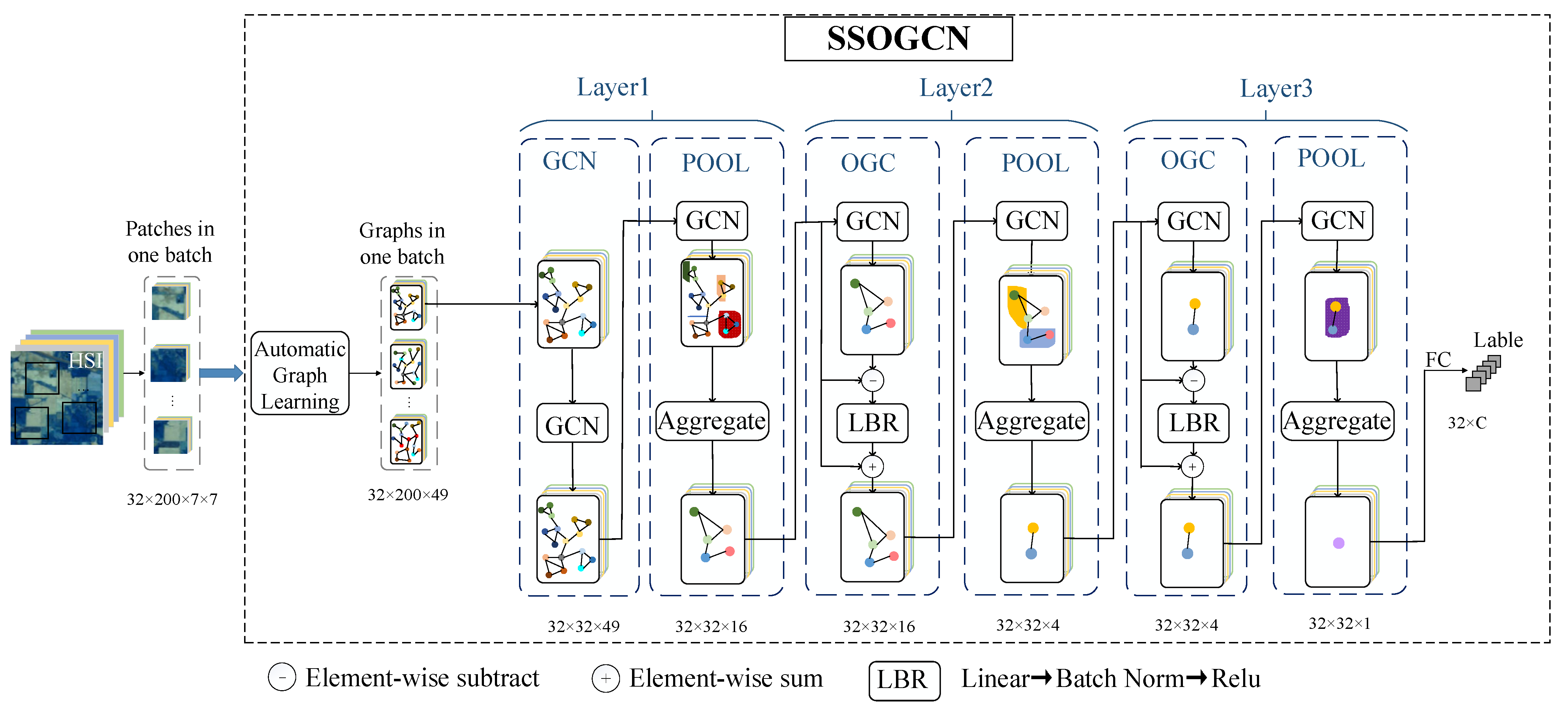
This section details the proposed HSI classification network SSOGCN, whose framework is shown in Figure 1. Taking HSI patches obtained through the square window around the central pixel as the input, the SSOGCN firstly construct each patch into a graph structure between pixels by automatic graph learning (AGL) module. Next, a three-layer GCN networks is designed to learn graph features. Each layer includes graph convolution/offset graph convolution (OGC) and graph pooling operation, which are used to extract features and aggregate information respectively. Finally, a full connect layer is used for classification. Our network is trained in an end-to-end way. In the following, we describe the key steps of our SSOGCN in details, including the AGL module (see Section 3.1) and the graph classification network (see Section 3.2).

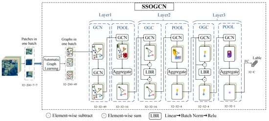
Figure 1. Framework of our SSOGCN.

3.1. Automatic Graph Learning (AGL)

Graphs are nonlinear data structures which can be utilized to describe complex relationships in non-Euclidean spaces. The relationships among HSI pixels are described as an undirected graph $G=(V,E)$, where $V$ is a vertex set composed of HSI pixels and $E$ is an edge set consisting of a series of weighted edge. An edge e_i,j denotes the similarity between any two nodes, i.e., $v_i$ and $v_j$. In our context, the adjacency matrix A of the undirected graph G, defines the relationships (or edges) among vertexes.

A general method of getting an undirected graph is to calculate the pairwise Euclidean distances between pixels. However, noises in HSI perhaps influence the quality of the obtained undirected graph and sequentially affect the subsequent task. Therefore, based on attention mechanism, we propose a AGL module which learn the graph structure in an automatic way and can be flexibly integrated to the classification model. Figure 2 details the process of obtaining the adjacency matrix $A$. Given the input patch with $n$ pixels and each pixels with a dimension $d_e$, we firstly perform linear transformation on input feature matrix $X\in {\Re }^{n\times d_e}$ as Equation (1), via weight matrixes $W_q,W_k\in {\Re }^{d_e\times d_a}$, to generate the query and key matrices $Q\in {\Re }^{n\times d_a},K\in {\Re }^{n\times d_a}$, respectively. We let $d_a=d_e/4$ for computational efficiency. Then, we utilize the query and key matrices to obtain the attention coefficients matrix $\stackrel{⌢}{A}$ by the matrix multiplication as shown in Equation (2). Finally, these attention coefficients are normalized by Equations (3) and (4) (denoted SS in Figure 2) to give $A=(\alpha )i,j$:

$$Q,K=X(W_q,W_k)$$

(1)

$$\stackrel{⌢}{A}=(\stackrel{⌢}{\alpha })i,j=Q{K}^T$$

(2)

$${\overline{\alpha }}_{i,j}=soft\max ({\stackrel{⌢}{\alpha }}_{i,j})=\frac{\exp ({\stackrel{⌢}{\alpha }}_{i,j})}{{\displaystyle \sum _k\exp ({\stackrel{⌢}{\alpha }}_{k,j})}}$$

(3)

$${\alpha }_{i,j}=\frac{{\overline{\alpha }}_{i,j}}{{\displaystyle \sum _k{\overline{\alpha }}_{i,k}}}$$

(4)

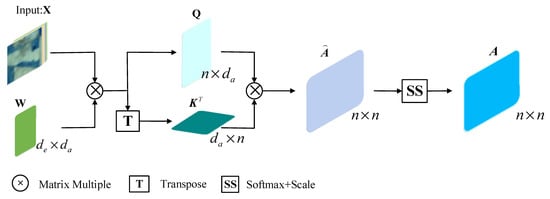
Figure 2. Automatic graph learning module (AGL).

In order to get more accurate graph embedding, it is necessary to only consider the connections between adjacent nodes. Therefore, the final adjacency matrix A of graph G can be obtained by Equation (5):

$$A=\{\begin{array}{l}{\alpha }_{i,j},\begin{array}{ccc}\begin{array}{cc}& if\end{array}& x_i\in Nei(x_j)& \begin{array}{cc}or& x_j\in Nei(x_i)\end{array}\end{array}\\ 0,\begin{array}{cc}& otherwise\end{array}\end{array}$$

(5)

Then, we can get the corresponding Laplacian matrix $L=D-A$ of graph G, where degrees matrix $D_{ii}={\displaystyle {\sum }_j{A}_{ij}}$ is a diagonal matrix. In Equation (6), the Laplace matrix $L$ is normalized and symmetrized to improve the generalization performance of the graph representation [66]:

$$L_{\mathrm{sym}}=D^{-1/2}L{D}^{-1/2}=I-D^{-1/2}A{D}^{-1/2}=U\Lambda U^T$$

(6)

where matrix I denotes the identity matrix, U is an orthogonal matrix comprised by the eigenvectors of the matrix L_sym, $\Lambda$ is a diagonal matrix comprised by eigenvalues of the matrix $L_{\mathrm{sym}}$.

3.2. Graph Classification Networks

This section details the proposed graph classification network. We train our network in the form of mini-batch. The input tensor size is 32 × 200 × 49, representing 32 undirected graphs ($G_1,G_2,\dots G_{32}$) in each batch. The size of vertex sets in each graph is 49, and D denotes the feature dimension of each vertex. Our graph classification network classifies each undirected graph into one category. Specific configuration of the network is shown in Table 1 below. We use GCN to reduce the dimension of the input and capture the structure information of the data in the first layer. OGC module we proposed is utilized to extract offset features in the second and third layers. In order to decrease the computational cost and improve the generalization performance of the model, we add a graph pooling layer after each feature extraction layer. The three graph pooling layers respectively sampled the number of nodes from 49, 16, 4 to 16, 4, 1. The fourth layer is the full connection layer, which maps the spectral-spatial features to the label space for classification. Next, we will detail the three major parts of the graph classification network: GCN, OGC, Graph pooling.

Table 1. Configuration of Deep Network Used in Graph Classification.

Layer	Module	Input Tensor Size	Output Tensor Size
1	GCN	32 × D × 49	32 × 32 × 49
	POOL	32 × 32 × 49	32 × 32 × 16
2	OGC	32 × 32 × 16	32 × 32 × 16
	POOL	32 × 32 × 16	32 × 32 × 4
3	OGC	32 × 32 × 4	32 × 32 × 4
	POOL	32 × 32 × 4	32 × 32 × 1
4	FC	32 × 32	32 × C

3.2.1. GCN

Given two sets of graph signals $x,g$ on graph G, the graph convolution operation is defined as Equation (7):

$$g★x=U[(U^{T}g)•(U^{T}x)]=U[\tilde{g}•(U^{T}x)]=(Udiag(\tilde{g})U^T)x=H_{\tilde{g}}x$$

(7)

where $★$ represents the graph convolution operation, and $•$ is the Hadamard product. Obviously, $H_{\tilde{g}}$ is a graph shift operator, whose frequency response matrix is the spectrum of $g$. The graph convolution operation equal to graph filter, and the core of the graph filter operator is the frequency response matrix. Joan et al. [25] parameterize the frequency response matrix. Let $g_{\theta }=diag(\theta )$, the graph convolution definition in Equation (7) can be further expressed as Equation (8):

$$g★x=U{g}_{\theta }{U}^{T}x$$

(8)

Eigenvector decomposition in Equation (8) has a heavy computational cost. Therefore, Hammond et al. fit any frequency response function approximately by the k-th order truncated expansion of Chebyshev polynomials [67], which is:

$$g_{{\theta }^{\prime }}(\Lambda )\approx {\displaystyle \sum _{k=0}^K{\theta }_k^{\prime }{T}_k(\tilde{\Lambda })}$$

(9)

where ${\theta }^{\prime }$ denotes a vector comprised by Chebyshev coefficients, and $\tilde{\Lambda }=2/({\lambda }_{\max })\Lambda -I$ which ${\lambda }_{\max }$ denotes the largest eigenvalue of matrix $L_{\mathrm{sym}}$. Therefore, Equation (8) can be written as Equation (10):

$$g_{{\theta }^{\prime }}★x\approx U{\displaystyle \sum _{k=0}^K{\theta }_k^{\prime }{T}_k(\tilde{\Lambda })}{U}^{T}x={\displaystyle \sum _{k=0}^K{\theta }_k^{\prime }{T}_k(\tilde{L})}x$$

(10)

where $\tilde{L}=2/({\lambda }_{\max })L_{\mathrm{sym}}-I$ is the scaled form of $L_{\mathrm{sym}}$. By limiting K = 1, Equation (10) is a linear function about Laplace matrix, so Kipf and Welling [14] make ${\lambda }_{\max }$ approximate to 2. The polynomial in Equation (10) can be further simplified as follows:

$$g_{\theta }★x\approx {\theta }_0^{\prime }x+{\theta }_1^{\prime }(L_{sym}-I)x=({\theta }_0^{\prime }-{\theta }_1^{\prime }{D}^{-\frac{1}{2}}A{D}^{-\frac{1}{2}})x$$

(11)

Let ${\theta }^{\prime } = {\theta }_0^{\prime }=-{\theta }_1^{\prime }$, then Equation (11) becomes:

$$g_{\theta }★x={\theta }^{\prime }(I+D^{-\frac{1}{2}}A{D}^{-\frac{1}{2}})x$$

(12)

where ${\theta }^{\prime }$ is a scalar, which is equivalent to doing a scale transformation on the frequency response function of $I+D^{-\frac{1}{2}}A{D}^{-\frac{1}{2}}$. Usually, such scale transformation will be replaced by the normalization operation in the neural network, so let ${\theta }^{\prime }=1$. However, deep GCN which operate Equation (12) repeatedly will suffer from exploding or vanishing gradients, since the eigenvalues of matrix $I+D^{-\frac{1}{2}}A{D}^{-\frac{1}{2}}$ range from 0 to 2. To prevent the training from getting worse, Kipf and Welling [35] took the renormalization trick denoted as $I+D^{-\frac{1}{2}}A{D}^{-\frac{1}{2}}\to {\widehat{D}}^{-\frac{1}{2}}\widehat{A}{\widehat{D}}^{-\frac{1}{2}}$, where $\widehat{A}=A+I$ and ${\widehat{D}}_{ii}={\displaystyle {\sum }_j{\widehat{A}}_{ij}}$. Therefore, the convolutional layer of GCN is defined in Equation (13):

$$H^{(l)}=\sigma ({\widehat{D}}^{-\frac{1}{2}}\widehat{A}{\widehat{D}}^{-\frac{1}{2}}{H}^{(l-1)}{W}^{(l)}+b^{(l)})$$

(13)

where matrix $H^{(l)}$ denotes the output features in the $l$th layer, $\sigma (•)$ is the nonlinear activation function (we choose Relu as the nonlinear activation function in our case), $W^{(l)}$ and $b^{(l)}$ denotes the trainable weight matrix and biases in the $l$th layer, respectively.

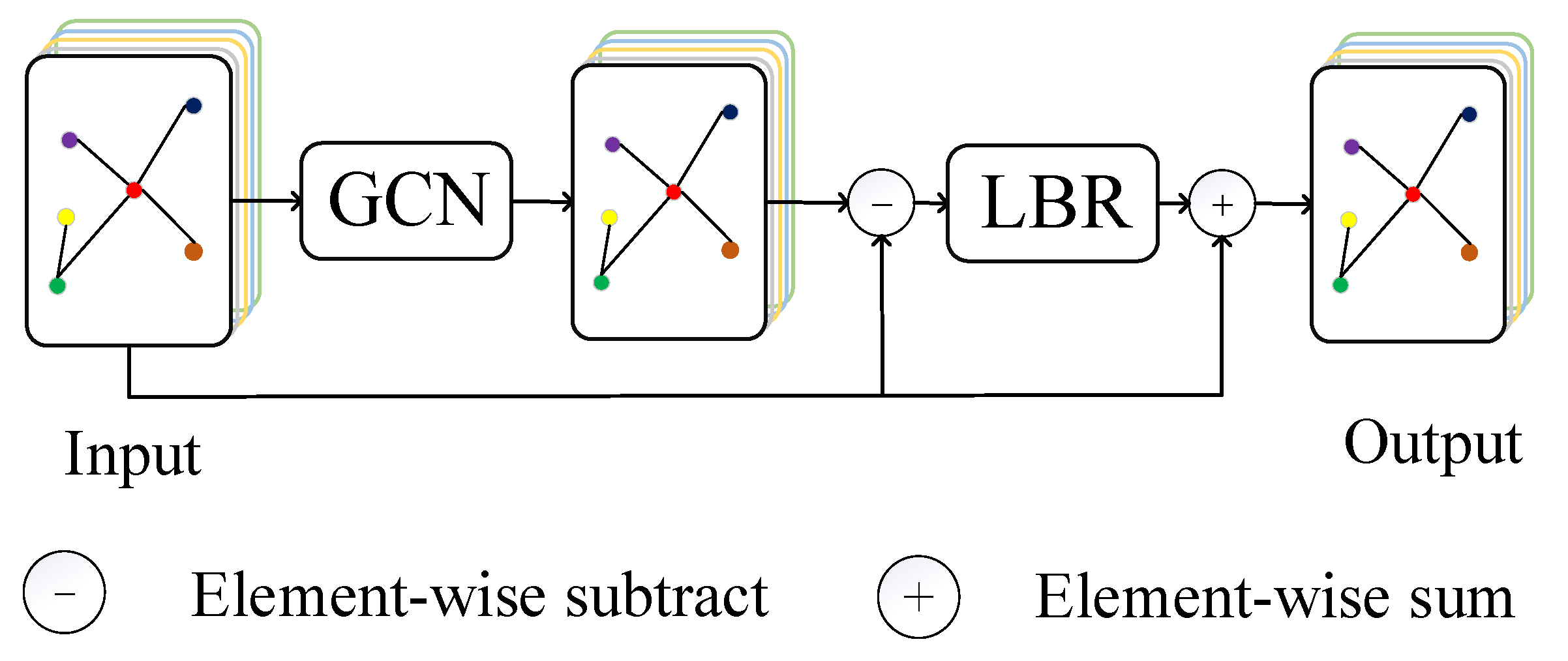
3.2.2. OGC

In order to emphasize important local spatial information and improve the classification performance of our model. we propose the offset graph convolution (OGC) module, and we replace the GCN layer with the OGC module. GCN is used to extract information among neighbor nodes. Therefore, the offset features between before and after extraction are the important information sent by the neighbor nodes. See Figure 3 for details, to obtain the offset features, we subtract the input features from the features extracted by GCN element by element, where the subtraction operator is equivalent to a filter. Next, we input the offset features into the LBR module which is combination of Linear, Batch Norm and Relu layers. Then, we add the input features of our module and the LBR output by element-wise. As shown in Equation (14):

$$H_{out}=OGC(H_{in})=LBR(H_{in}-H_{GCN})+H_{in}$$

(14)

where H_in is the input of OGC module, H_out is the output of OGC module and H_GCN is the output of GCN. According to the definition of GCN layer in Equation (13), we can get:

$$\begin{array}{l}{H}_{in}-H_{GCN}=H_{in}-({\widehat{D}}^{-\frac{1}{2}}\widehat{A}{\widehat{D}}^{-\frac{1}{2}}{H}_{in}W+b)\\ \approx H_{in}-{\widehat{D}}^{-\frac{1}{2}}\widehat{A}{\widehat{D}}^{-\frac{1}{2}}{H}_{in}=(I-{\widehat{D}}^{-\frac{1}{2}}\widehat{A}{\widehat{D}}^{-\frac{1}{2}})H_{in}=({\widehat{D}}^{-\frac{1}{2}}\widehat{L}{\widehat{D}}^{-\frac{1}{2}})H_{in}={\widehat{L}}_{sym}{H}_{in}\end{array}$$

(15)

where matrix W and vector b are negligible as the weight matrix and bias term in linear transformation, and ${\widehat{L}}_{sym}$ is the regularization Laplace matrix of $\widehat{A}$ with $\widehat{A}=A+I$. Rather, $\widehat{A}=A+I$ is equivalent to adding a self-connection to the adjacency matrix to emphasize the information of each node itself. Therefore, $H_{in}-H_{GCN}$ can be approximated to the Laplace smoothing operation to the input. According to the row vector perspective of matrix multiplication, ${\widehat{L}}_{sym}{H}_{in}$ is equivalent to aggregate the important feature within neighbor nodes.

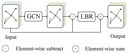
Figure 3. Offset graph convolution module (OGC).

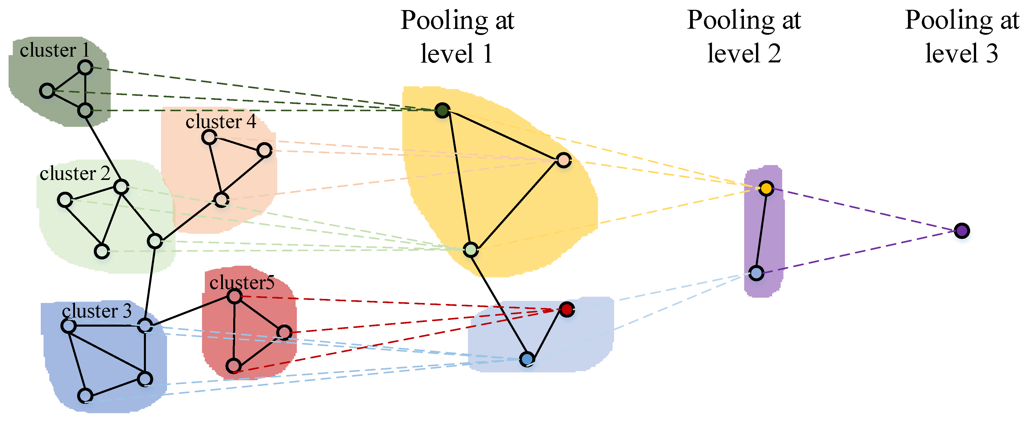
3.2.3. Graph Pooling

Besides extracting the features through GCN layer, another important part in graph classification network is the aggregation of global features by the pooling layer. Graph classification based on global pooling loses rich structural information in the graph data, since it regards inputs as flat data and all nodes are treated equally. Therefore, we adopt the layer-wise hierarchical pooling [68] to aggregate the global features. Figure 4 illustrates a simple three-layer graph pooling process. Specifically, the input nodes are firstly formed into a set of subgraphs by clustering. Then these subgraphs are treated as a set of super-nodes and gradually merged into one node. The hierarchical pooling has many advantages such as decreasing the computational cost and learning the rich structure information of the graph data. Our graph pooling has two major steps. Firstly, as shown in Equation (16), we utilize GCN to learn a cluster assignment matrix which can describes the probability that each node belongs to a certain cluster. The second step is to aggregate the nodes in each cluster by Equation (17) to get the output $H^{(l+1)}$ of the pooling layer:

$$S^{(l)}=soft\max (GCN(A^{(l)},H_{out}^{(l)}))$$

(16)

$$H^{(l+1)}={(S^{(l)})}^T{H}_{out}^{(l)}$$

(17)

where $S^{(l)}\in {\Re }^{n\times m}$ is a soft assignment of each node in the l-th layer. $n$ is the number of nodes in the l-th layer, $m$ is the number of nodes in the (l + 1)-th layer.

Figure 4. Three-layer pooling process.

4. Experiment

4.1. Data Sets

Three representative HSI data sets which cover different areas are adopted to evaluate the performance of the SSOGCN method: the Indian Pines data set, Pavia University data set and Salinas data set.

(1)

Indian Pines Data Set: The scene over northwestern Indiana, USA was acquired over the Airborne Visible/Infrared Imaging Spectrometer (AVIRIS) sensor in 1992. The image consists of 145 × 145 pixels and the spatial resolution is 20 m per pixel.

There are 220 bands in the range of 0.4~2.5, and 200 bands are available after getting rid of the bands with serious noise effects. The data set contains 16 types of features, and 10,249 sample data can be referred. The false color map and ground-truth map are shown in Figure 5. Table 2 lists 16 main land-cover categories involved in this scene, as well as the number of training and testing samples used for our experiments.

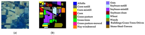
Figure 5. Indian Pines Data Set ((a) False-color map; (b) Ground-truth map).

Table 2. Number of training and test sets for the Indian Pines data set.

Class	Class Name	Train	Test
1	Alfalfa	15	31
2	Corn-notill	50	1378
3	Corn-mintill	50	780
4	Corn	50	187
5	Grass-pasture	50	433
6	Grass-trees	50	680
7	Grass-pasture-mowed	15	13
8	Hay-windrowed	50	428
9	Oats	15	5
10	Soybean-notill	50	922
11	Soybean-mintill	50	2405
12	Soybean-clean	50	543
13	Wheat	50	155
14	Woods	50	1215
15	Buildings-Grass-Trees-Drives	50	336
16	Stone-Steel-Towers	50	43
	Total	695	9554

(2)

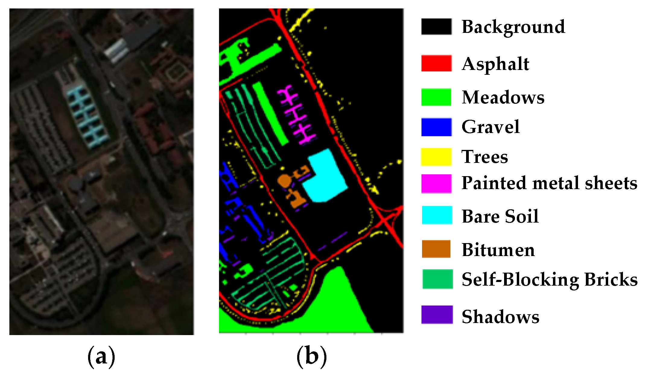
Pavia University Data Set: The second image comprised by 610 × 340 pixels and each pixel are 1.3 m. It was acquired by the Reflective Optics System Imaging Spectrometer (ROSIS) sensor in 2002. There are 115 bands in the range of 0.43~0.86, and 103 bands without serious noise are selected for experiment. The data set includes nine land cover classes, and a total of 42,776 samples can be referred. As shown in Figure 6 below, the left image is a false color map, the middle column is a ground-truth map, and the right is the corresponding class name. Table 3 lists 9 major land-cover classes in this image, as well as the number of training and testing samples used for our experiments.

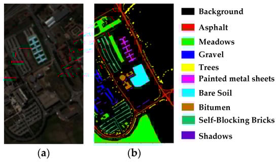Figure 6. Pavia University Data Set ((a) False-color map; (b) Ground-truth map).

Table 3. Number of training and test sets for the Pavia University data set.

Class	Class Name	Train	Test
1	Asphalt	50	6581
2	Meadows	50	18,599
3	Gravel	50	2049
4	Trees	50	3014
5	Painted metal sheets	50	1295
6	Bare Soil	50	4979
7	Bitumen	50	1280
8	Self-Blocking Bricks	50	3632
9	Shadows	50	897
	Total	450	42,326

(3)

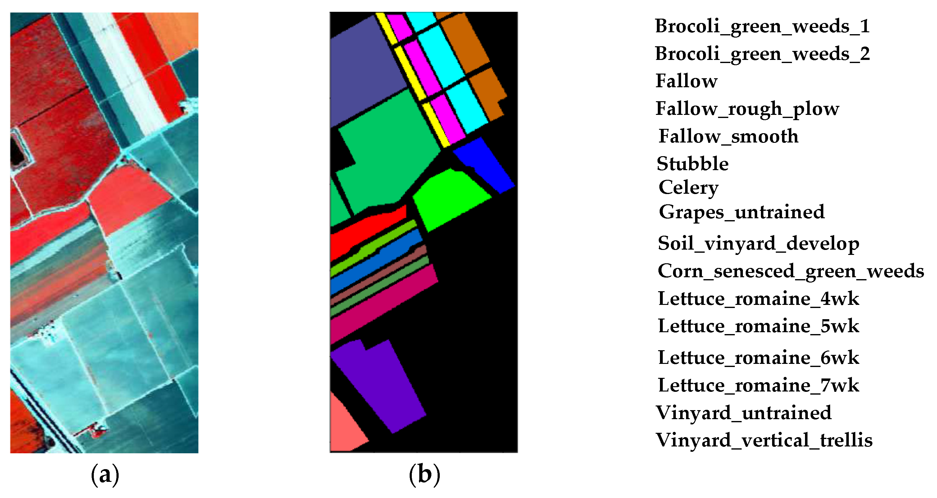
Salinas Data Set: The scene over Salinas Valley, California was acquired the AVIRIS sensor. The image consists of 512 × 217 pixels and the spatial resolution is 3.7 m per pixel. There are 204 bands are available after discarding the 20 water absorption bands. The data set contains 16 types of features, and 54,129 samples can be referred. Table 4 lists 16 main land-cover categories involved in this scene, as well as the number of training and testing samples used for our experiments. The false color map and ground-truth map are shown in Figure 7.

Table 4. Number of training and test sets for the Salinas data set.

Class	Class Name	Train	Test
1	Brocoli_green_weeds_1	50	1959
2	Brocoli_green_weeds_2	50	3676
3	Fallow	50	1926
4	Fallow_rough_plow	50	1344
5	Fallow_smooth	50	2628
6	Stubble	50	3909
7	Celery	50	3529
8	Grapes_untrained	50	11,221
9	Soil_vinyard_develop	50	6153
10	Corn_senesced_green_weeds	50	3228
11	Lettuce_romaine_4wk	50	1018
12	Lettuce_romaine_5wk	50	1877
13	Lettuce_romaine_6wk	50	866
14	Lettuce_romaine_7wk	50	1020
15	Vinyard_untrained	50	7218
16	Vinyard_vertical_trellis	50	1757
	Total	800	53,329

Figure 7. Salinas Data Set ((a) False-color map; (b) Ground-truth map).

4.2. Experimental Settings

In the experiment, we used Pytorch 1.6 framework to implement the HSI classification networks. All experiments were run on RTX 2080Ti GPU with Python 3.7.3, CUDA 10.2.

We randomly selected 50 labeled samples from each class as training samples, or 15 labeled samples per class if the number of samples in a class is less than 50 samples, and the rest samples were used as the test sets. For training, Adam optimizer was utilized to optimize all models. The cross-entropy loss function was chosen to measure classification error. The weight decay was empirically set to 0.001. The learning rate was initialized to 0.01, and dropped to 0.1 times for every 50 epochs. The training task was completed after 200 epochs with a batch size setting to 32.

We chose eight SOTA methods applied to the field of HSI classification task recently as comparative approaches to verify the classification capability of SSOGCN from multiple perspectives. Specifically, we compared two traditional methods (KNN [69] and SVM [70]), two CNN-based methods (2D-CNN [71] and CNN-PPF [48]), three GCN-based methods (GCN [14], miniGCN [20], MDGCN [18]), and the method based on CNN and GCN (FuNet-C [20]). The parameter configurations of all comparative methods were consistent with those in the reference of comparison methods. Three classic indicators including overall accuracy (OA), average accuracy (AA) and kappa coefficient (KA) were utilized to assess the algorithm quantitatively. All of these methods were run ten times on each dataset, and the average accuracies were reported.

4.3. Classification Results

4.3.1. Results on the Indian Pines Data Set

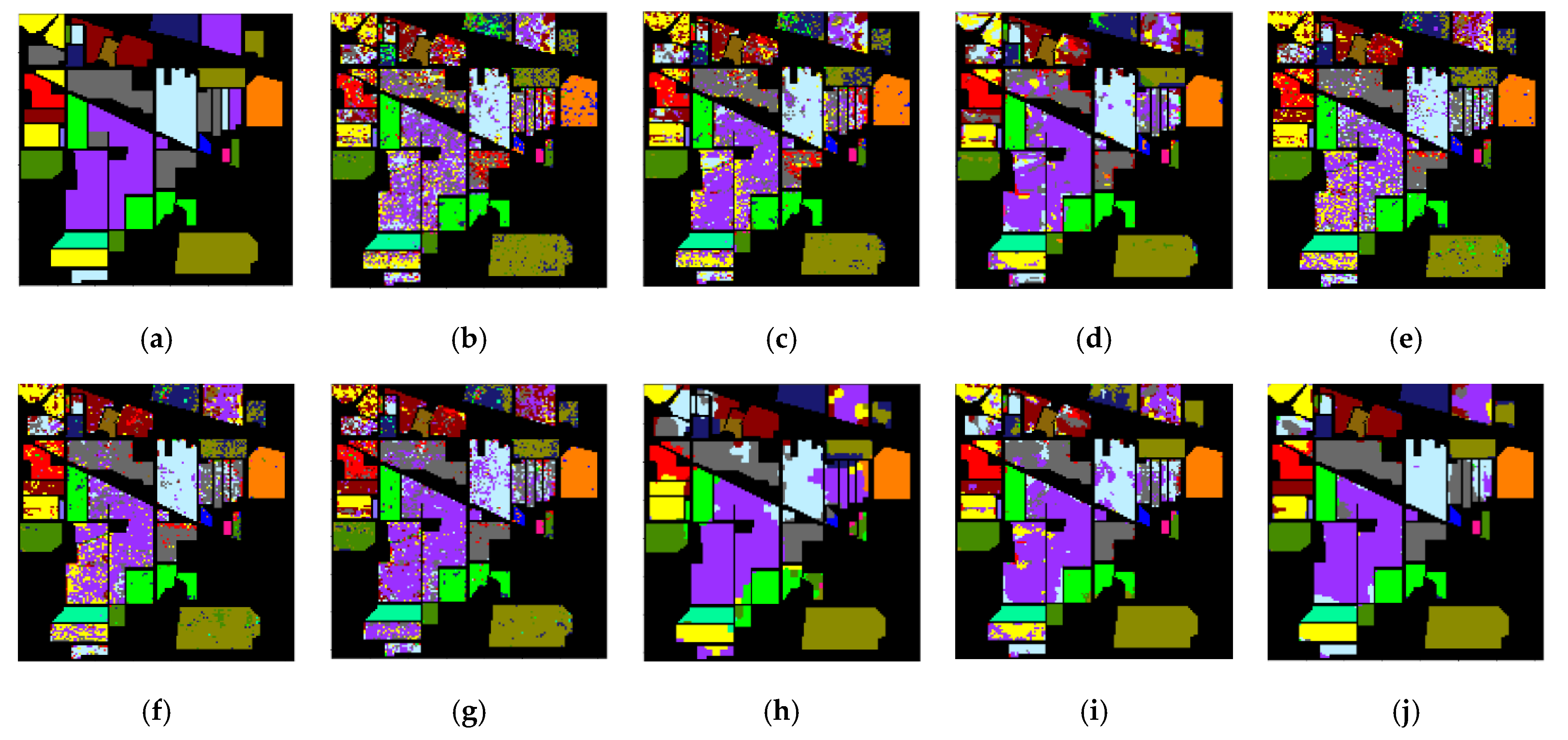
The quantitative results on the Indian Pines data set are summarized in Table 5, where the highest value in each row is highlighted in bold. It can be seen that our methods are improved by 17.81%, 21.18% in OA, respectively, compared with GCN, miniGCN, which mainly model long-range spatial relationships and ignore local spatial information. In addition, it has a great improvement in OA compared with 2D-CNN which is restricted by the fixed convolution kernel.

Table 5. Classification performance of various methods in Indian Pines data set (%).

Class	KNN	SVM	2D-CNN	CNN-PPF	GCN	miniGCN	MDGCN	FuNet-C	SSOGCN
1	15.54	16.89	12.03	16.22	18.92	17.57	93.54	29.59	20.95
2	45.79	68.94	70.6	67.49	75.47	68.07	65.82	78.81	87.52
3	54.87	57.56	68.25	55.38	62.05	53.97	83.33	84.49	93.46
4	63.64	79.68	99.52	78.07	86.63	66.84	96.25	96.26	100.0
5	84.30	89.15	94.48	89.61	88.68	77.37	79.44	97.92	98.38
6	87.65	91.32	100.0	92.50	94.85	93.38	92.05	99.12	98.68
7	92.31	92.31	100.0	100.0	100.0	100.0	23.07	100.0	100.0
8	89.72	95.09	97.1	96.73	97.20	98.36	100.0	100.0	100.0
9	80.00	100.0	100.0	100.0	100.0	80.00	0.00	100.0	100.0
10	67.68	77.66	75.58	74.51	80.48	69.52	73.53	85.25	92.41
11	49.94	59.09	70.8	63.58	59.58	63.04	88.77	78.50	90.19
12	44.94	62.80	65.72	78.08	79.56	64.64	67.77	79.74	95.76
13	96.13	98.06	100.0	100.0	98.71	98.06	100.0	100.0	99.35
14	74.65	80.00	89.15	84.44	80.41	86.17	92.02	96.30	97.12
15	52.98	71.43	84.27	76.19	80.06	69.64	96.43	89.29	99.11
16	93.02	93.02	100.00	97.67	95.35	90.70	83.72	100.0	100.0
OA(%)	61.06	71.20	78.93	73.42	74.7	71.33	80.53	85.54	92.51
AA(%)	68.32	77.06	83.32	79.41	81.12	74.83	77.23	87.83	92.06
KA(%)	56.29	67.60	76.10	69.91	71.47	67.42	81.11	83.52	91.45

As shown in Figure 8, the SSOGCN proposed in this paper has fewer error points in the classification graph. It is worth noting that the classification accuracy on category 9 of MDGCN, which is based on super-pixel segmentation, is 0. MDGCN thinks all pixels in a super-pixel should belong to the same category. So, if the super-pixel is in the wrong category, a large number of pixels in the super-pixel block will be misclassified.

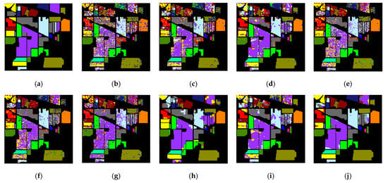
Figure 8. Classification map of various algorithms in the Indian Pines data set ((a) Gound-truth map; (b) KNN; (c) SVM; (d) 2D-CNN; (e) CNN-PPF; (f) GCN; (g) miniGCN; (h) MDGCN; (i) FuNet-C; (j) SSOGCN).

4.3.2. Results on the Pavia University Data Set

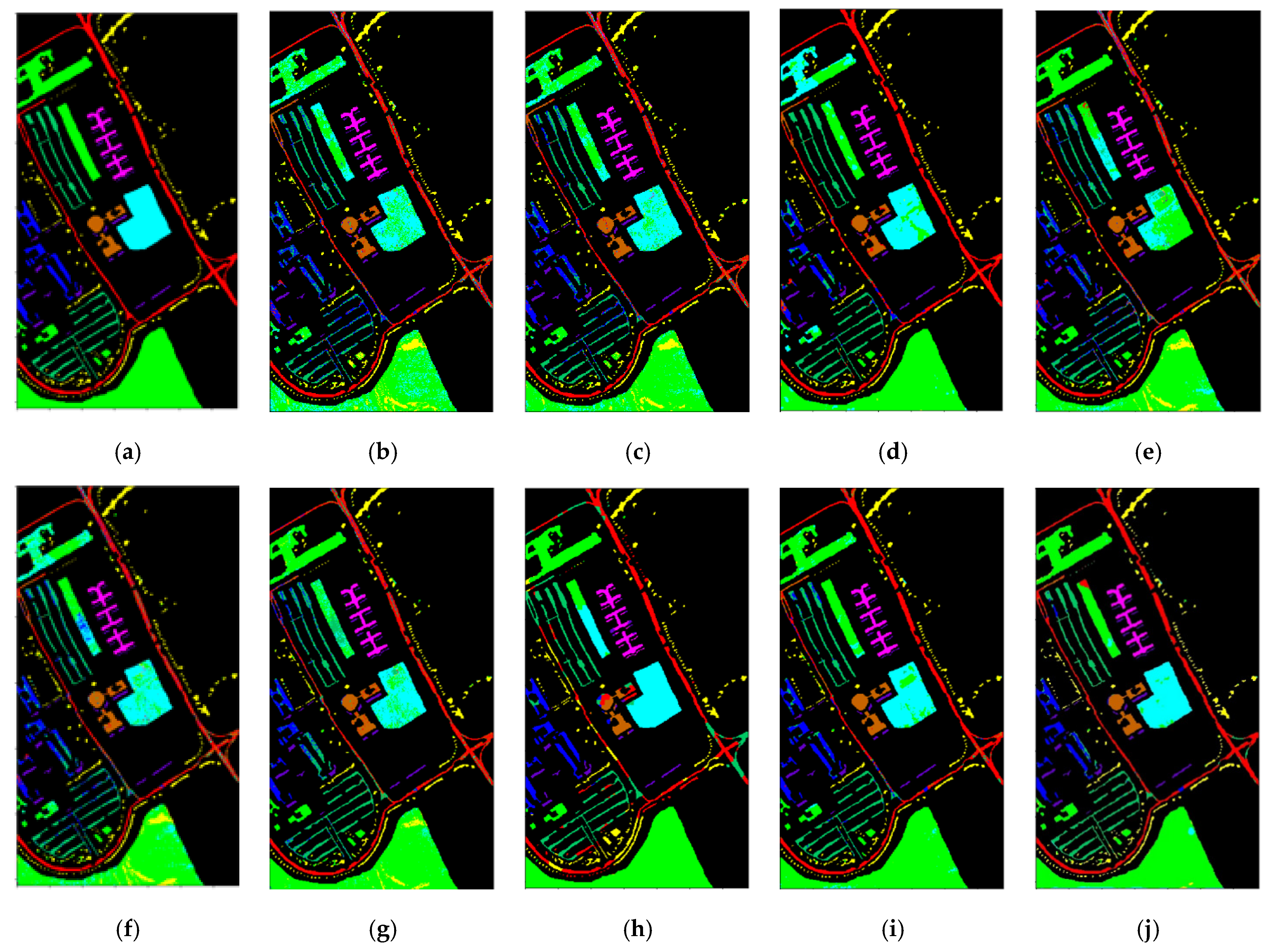
Table 6 demonstrates the quantitative results on the Pavia University data set in details, which are similar to those in the Indian Pines data set. It can be seen apparently that our SSOGCN gains the highest OA, AA, and KA than those in all other SOTA algorithms. Moreover, the classification accuracy of each method on the University of Pavia data set is higher than that in the Indian Pines due to less noises within the data set.

Table 6. Classification performance of various algorithms in Pavia University data set (%).

Class	KNN	SVM	2D-CNN	CNN-PPF	GCN	miniGCN	MDGCN	FuNet-C	SSOGCN
1	67.45	63.07	76.10	57.73	64.03	78.62	62.80	85.34	95.00
2	70.88	82.59	83.52	83.56	83.42	86.77	88.67	95.33	99.09
3	67.01	81.80	75.40	82.97	78.09	70.82	93.76	91.65	84.58
4	88.12	90.44	97.51	89.28	89.25	88.49	81.89	96.95	95.92
5	98.92	99.61	99.46	99.00	98.61	98.53	97.17	99.92	99.77
6	69.05	82.43	78.53	54.35	86.10	81.74	99.22	90.76	97.23
7	87.97	92.11	94.77	93.52	90.47	90.16	85.19	97.89	98.28
8	71.97	78.85	84.55	62.89	79.87	83.07	79.79	88.79	96.26
9	100.0	99.89	100.0	100.0	100.0	100.0	53.33	100.0	99.89
OA(%)	73.26	80.44	83.65	75.35	81.14	84.69	84.24	92.93	97.08
AA(%)	80.15	85.64	87.76	80.36	85.54	86.47	82.37	94.07	96.22
KA(%)	65.96	74.96	78.79	67.64	75.84	79.99	79.57	90.66	96.11

As shown in Figure 9, the classification maps obtained by our SSOGCN method is more consistent with the ground-truth map. Specifically, from Figure 9f,g,i,j, it can be seen that GCN, miniGCN, FuNet-C, and SSOGCN, which use GCN, have fewer misclassification points in the class boundary region. However, from Figure 9h, it can be seen that MDGCN which is also based on GCN has more misclassification points due to the inaccurate super-pixel segmentation.

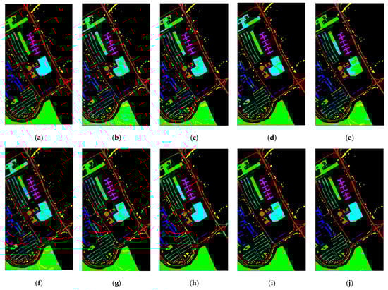
Figure 9. Classification map of various algorithms in the Pavia University data set ((a) Gound-truth map; (b) KNN; (c) SVM; (d) 2D-CNN; (e) CNN-PPF; (f) GCN; (g) miniGCN; (h) MDGCN; (i) FuNet-C; (j) SSOGCN).

4.3.3. Results on the Salinas Data Set

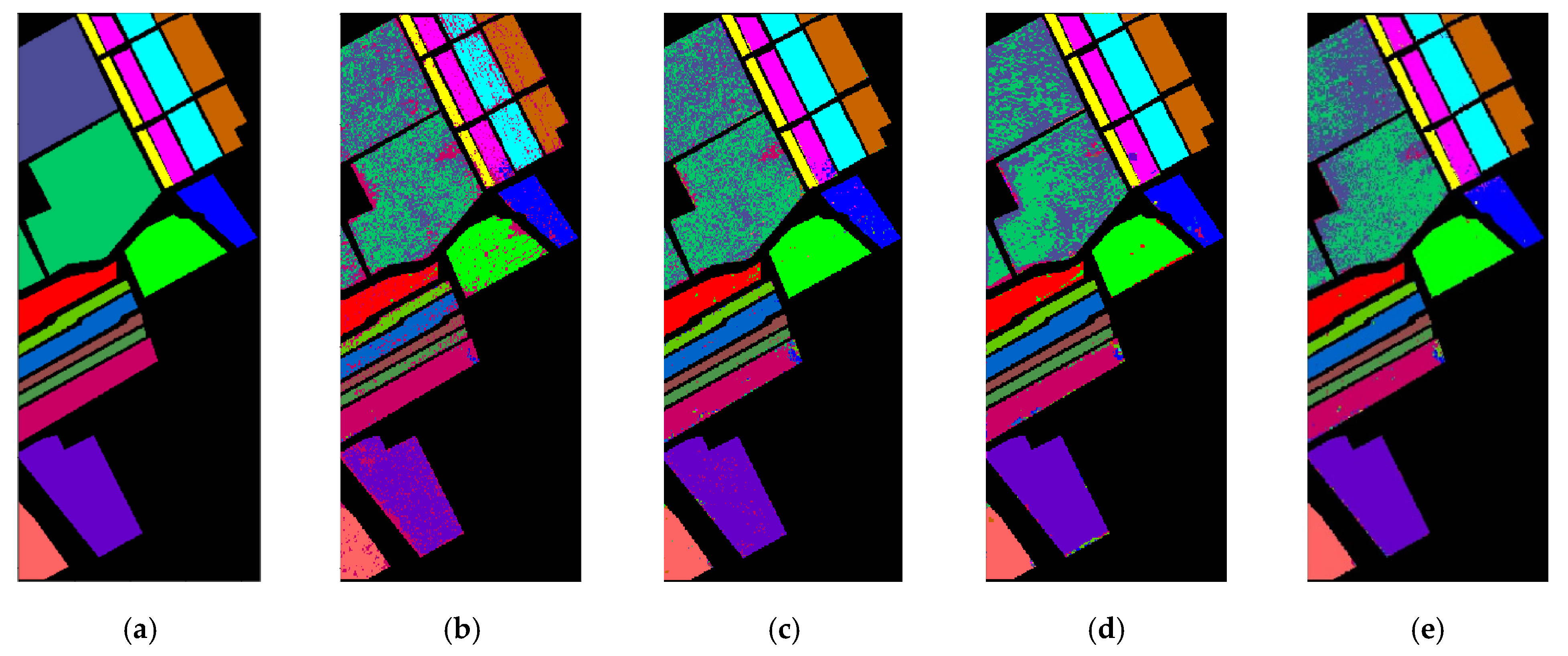
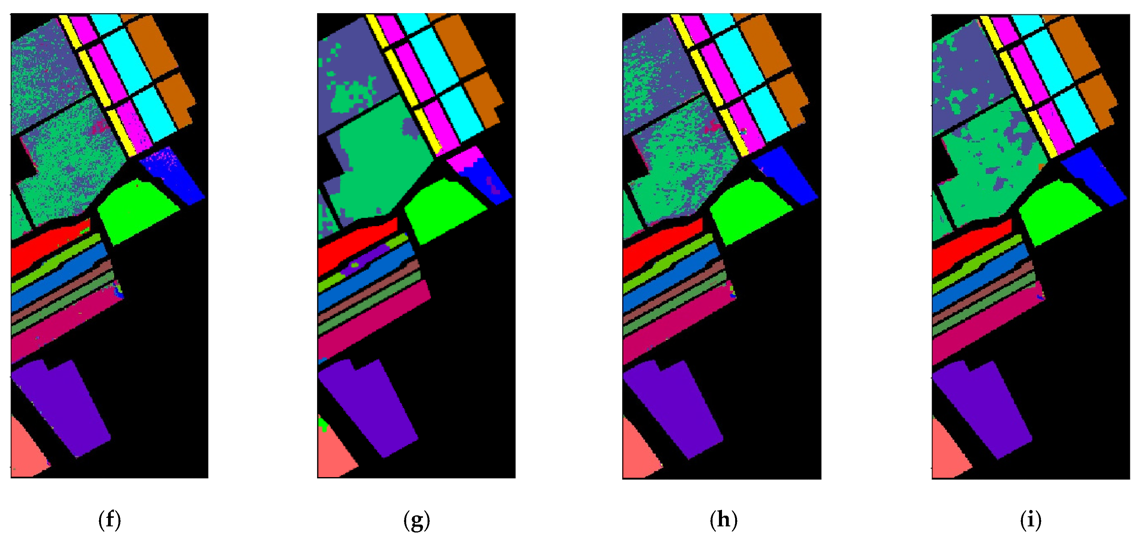
Table 7 exhibits the quantitative results on the Salinas dataset. Obviously, OA, AA and KA obtained by our SSOGCN are still the highest, compared with other SOTA algorithms. The methods based on deep learning own higher classification accuracy than traditional machine learning methods (KNN, SVM). In addition, due to the high spatial resolution and spectral dimension, the GCN-based method named GCN occurs out of memory when we calculate the adjacency matrix. Our SSOGCN method effectively solved this problem and won superior classification performance. It is obvious from Figure 10 that the classification map of SSOGCN shows fewer error points.

Table 7. Classification performance of various methods in Salinas data set (%).

Class	KNN	SVM	2D-CNN	CNN-PPF	miniGCN	MDGCN	FuNet-C	SSOGCN
1	88.42	97.13	95.61	85.15	97.60	100.0	100.0	100.0
2	88.25	97.08	97.03	99.97	99.89	100.0	99.97	100.0
3	93.82	91.49	96.0	94.65	93.87	63.11	99.22	99.88
4	90.48	99.56	99.55	99.63	99.03	97.06	99.55	99.75
5	83.87	92.84	96.88	97.41	97.45	99.74	97.34	97.26
6	82.02	99.72	99.39	99.82	99.97	100.0	100.0	100.0
7	87.79	99.3	99.12	99.60	99.63	100.0	99.43	100.0
8	50.84	57.58	51.38	92.06	67.13	85.47	64.46	83.12
9	81.75	97.69	97.40	99.58	99.38	100.0	99.93	99.80
10	97.40	85.0	90.68	89.71	92.13	98.66	97.15	97.84
11	78.09	92.81	98.13	93.03	97.35	48.78	99.71	99.45
12	87.16	98.74	99.89	99.73	99.89	100.0	100.0	99.94
13	88.34	99.10	99.65	99.77	99.54	100.0	100.0	100.0
14	80.29	90.81	98.63	93.24	98.14	99.63	98.92	100.0
15	63.52	52.01	66.42	23.04	70.16	81.84	76.20	91.99
16	89.53	93.66	97.10	98.01	98.41	93.36	98.69	99.94
OA(%)	76.05	81.84	83.41	85.98	87.85	91.72	88.84	95.05
AA(%)	83.22	90.28	92.68	91.52	94.35	91.70	95.66	98.06
KA(%)	73.52	79.85	81.62	84.27	86.5	90.77	87.61	94.49

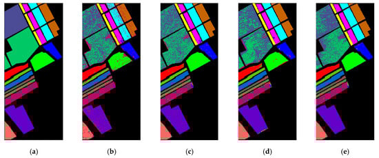
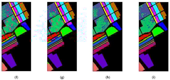
Figure 10. Classification map of various algorithms in the Salinas data set ((a) Gound-truth map; (b) KNN; (c) SVM; (d) 2D-CNN; (e) CNN-PPF; (f) miniGCN; (g) MDGCN; (h) FuNet-C; (i) SSOGCN).

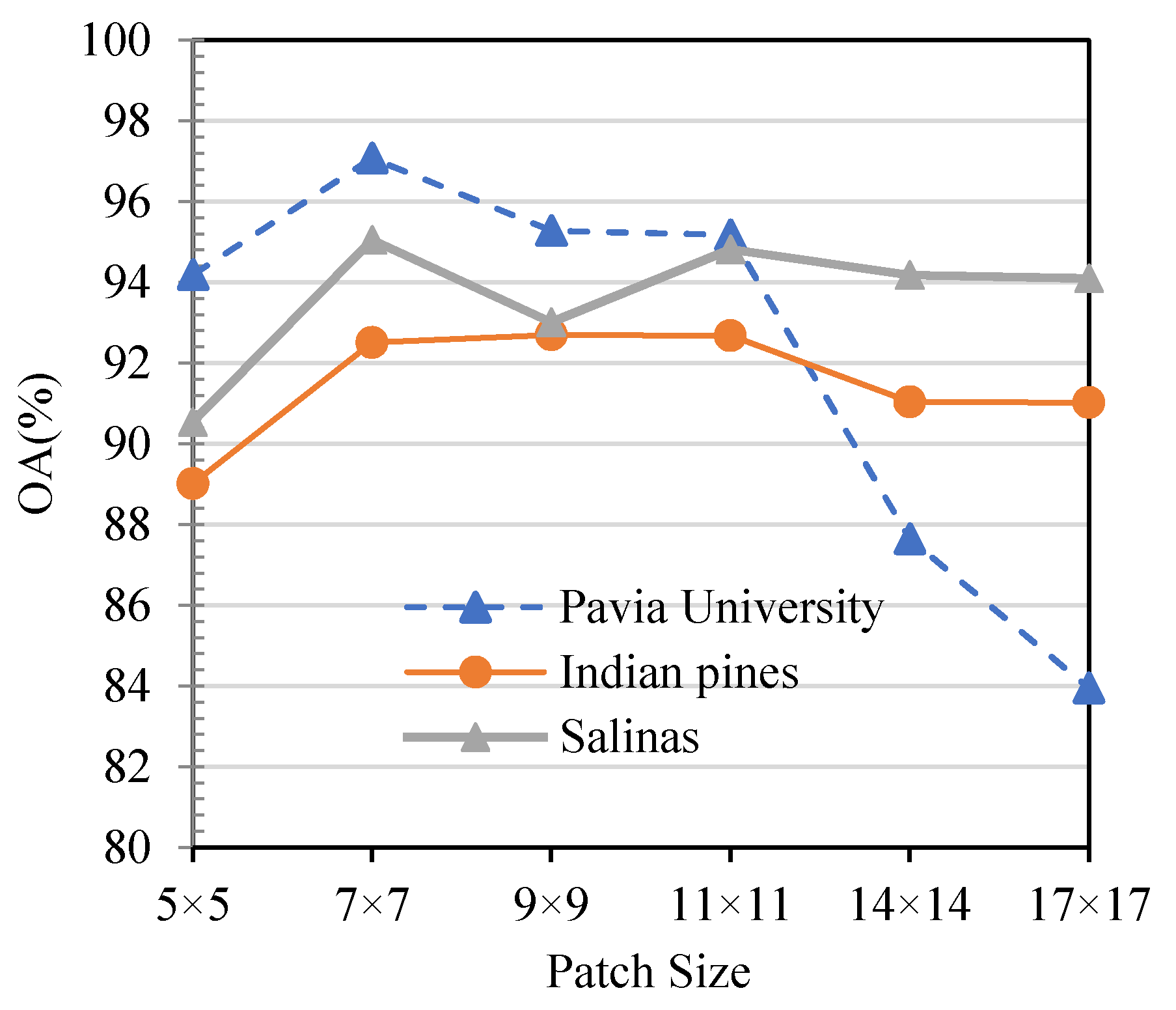
4.4. Impact of Patch Size

In our proposed method, we input a HSI patch, whose dimensionality is high. It will have a high computation cost if the input patch is too large, while it will miss important information if the input patch is too small. Therefore, we analyze the effect of different input sizes in this section. As shown in Figure 11, with the increase of the patches size, the overall accuracy first increased rapidly and then decreased since more information which is not conducive to classification is included.

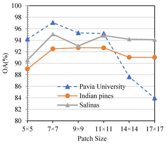
Figure 11. Parameter Sensitivity Analysis.

This phenomenon is particularly evident in the Pavia University data set, in which the ground-object has a fairly irregular distribution. Therefore, the patch size in each dataset is uniformly set to 7 × 7 in our experiment according to Figure 11.

4.5. Ablation Study

This section investigates the usefulness of these three operations: automatic graph learning module, offset graph convolution module and graph pooling, where the experimental setup stays the same as the abovementioned experiments in Section 4.3. Table 8 clearly indicates that the OA of SSOGCN improved 1.13%, 3.04% and 1.2% compared with the situation without AGL in the three datasets, i.e., Indian Pines, Pavia University and Salinas data set, respectively. It indicates that the automatic graph learning module we propose learned an optimal graph structure for the downstream task. In addition, SSOGCN improves the OA by 2.39% and 2.17%, 1.31% compared the situation without OGC in Indian Pines, Pavia University and Salinas data set, respectively, which demonstrates the effectiveness of the offset graph convolution module. Moreover, we can see from Table 8, the OA decrease 5.86%, 3.61%, and 6.45% in the Indian Pines, Pavia University and Salinas data set when we remove graph pooling module. It shows that the graph pooling has a good efficiency on learning graph structure and reducing dimensions.

Table 8. Ablation study (%).

Data Set	Without OGC	Without AGL	Without Graph Pooling	SSOGCN
Indian Pines	90.12	91.38	86.65	92.51
Pavia University	94.91	94.04	93.47	97.08
Salinas	93.74	93.85	88.60	95.05

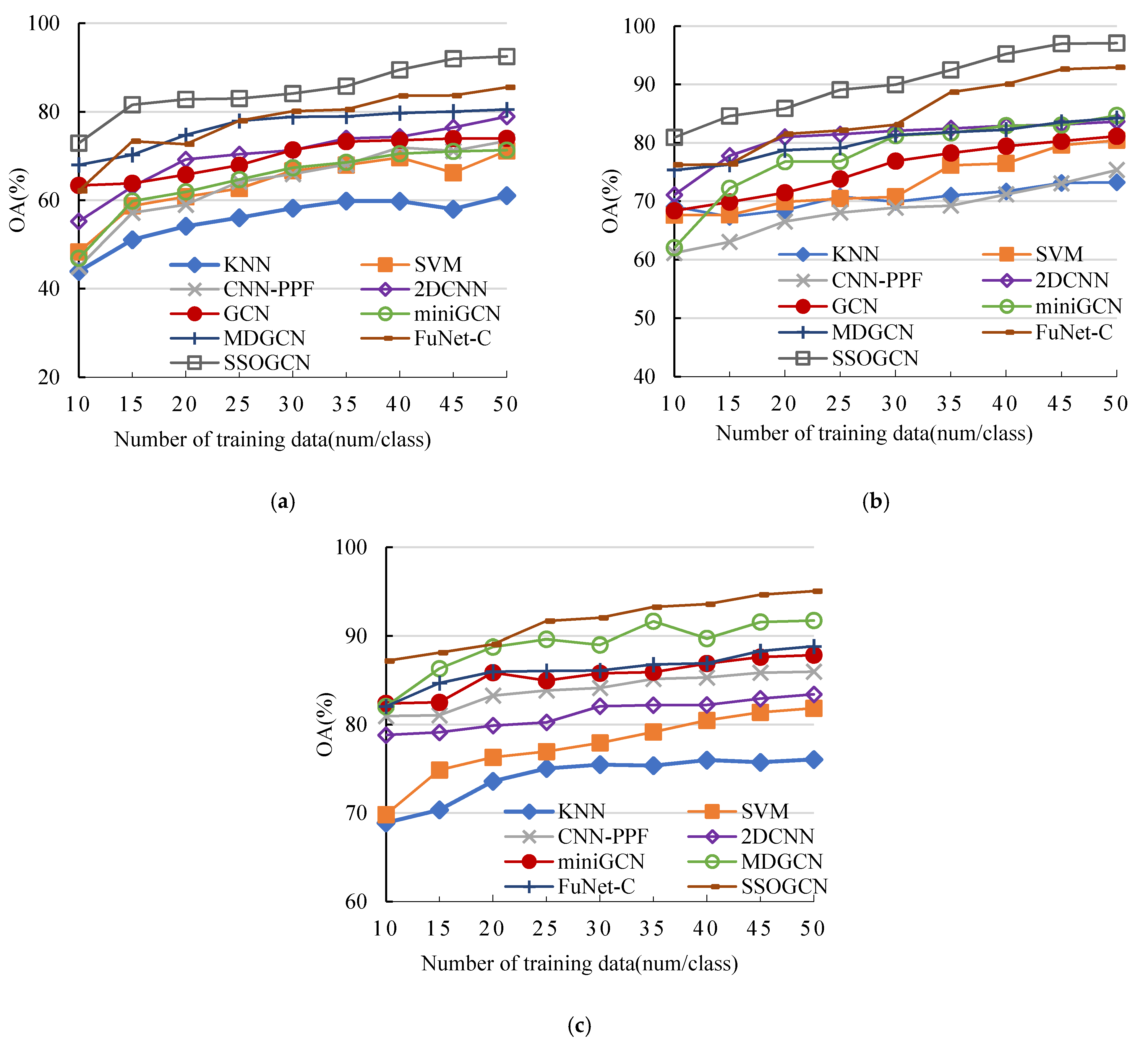
4.6. Impact of the Number of Labeled Samples

In this section, we analyze the sensitivity of each algorithm to the number of labeled samples. We vary the number of labeled samples per class from 10 to 50 with an interval of 5. As can be seen from Figure 12a–c, the classification accuracy of all methods is improved with the increase of the number of labeled samples in three data sets, which indicates that more labeled examples contain more information contribute to classification. It is also noteworthy that SSOGCN grow fast at the early stage and the grow slowly at late stage, and SSOGCN always stay at the highest accuracy compared with other SOTA methods. These results demonstrate the effectiveness and stability of the SSOGCN method.

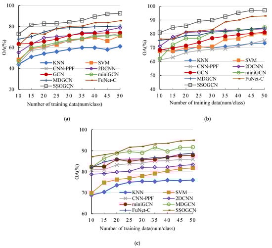
Figure 12. Sensitivity analysis of training set size. (a) Indian Pines data set. (b) Pavia University data set. (c) Salinas data set.

4.7. Running Time

The time consumed for training of each method on the Indian Pines, the Pavia University and Salinas data sets is shown in Table 9, Table 10 and Table 11 The GCN-based method takes more time than the CNN-based method on three data sets because the computation of the adjacency matrix is still a time-consuming step, but as a whole, it seems that the training time cost of SSOGCN is acceptable compared with FuNet-C.

Table 9. Run time comparison and parameter number comparison of depth model in the Indian Pines data set.

Methods	Time (s)	Params (K)
2D-CNN	178.06	30.0
CNN-PPF	61.86	44.82
GCN	198.12	4.36
miniGCN	776.86	28.70
MDGCN	322.01	13.07
FuNet-C	678.13	148.59
SSOGCN	597.05	23.41

Table 10. Run time comparison and parameter number comparison of depth model in the Pavia University data set.

Methods	Time (s)	Params (K)
2D-CNN	167.65	29.10
CNN-PPF	149.18	31.50
GCN	410.38	2.27
miniGCN	2925.70	15.19
MDGCN	447.87	6.81
FuNet-C	2753.58	77.44
SSOGCN	1471.03	12.22

Table 11. Run time comparison and parameter number comparison of depth model in the Salinas University data set.

Methods	Time (s)	Params (K)
2D-CNN	283.94	30.00
CNN-PPF	243.28	45.32
miniGCN	1273.54	29.22
MDGCN	458.48	13.31
FuNet-C	5002.85	150.264
SSOGCN	1183.93	23.96

Meanwhile, it is also noteworthy that the parametric number of the convolutional neural networks is larger, while the graph convolutional neural networks effectively reduce the number of parameters.

5. Conclusions

In this paper we have developed a novel HSI classification method termed SSOGCN. Unlike previous work that constructs adjacency matrices based on all data, our method constructs an adjacency matrix based on pixels within the input patch, and we construct a graph classification network to extract spectral-spatial features of HSI and classify the patch. Moreover, an offset graph convolution module is employed to emphasize local spatial information. As a result, our SSOGCN significantly reduces the computational effort and extracts the rich local spatial information within the patch, which can effectively alleviate the problem of inaccurate classification caused by spectral variability. The experimental results on three classical data sets show that our proposed method has better classification performance than the SOTA methods.

References

- Li, W.; Feng, F.; Li, H.; Du, Q. Discriminant Analysis-Based Dimension Reduction for Hyperspectral Image Classification: A Survey of the Most Recent Advances and an Experimental Comparison of Different Techniques. IEEE Geosci. Remote Sens. Mag. 2018, 6, 15–34. [Google Scholar] [CrossRef]
- Yin, J.; Qi, C.; Chen, Q.; Qu, J. Spatial-Spectral Network for Hyperspectral Image Classification: A 3-D CNN and Bi-LSTM Framework. Remote Sens. 2021, 13, 2353. [Google Scholar] [CrossRef]
- Yan, H.; Wang, J.; Tang, L.; Zhang, E.; Yan, K.; Yu, K.; Peng, J. A 3D Cascaded Spectral–Spatial Element Attention Network for Hyperspectral Image Classification. Remote Sens. 2021, 13, 2451. [Google Scholar] [CrossRef]
- Pu, S.; Wu, Y.; Sun, X.; Sun, X. Hyperspectral Image Classification with Localized Graph Convolutional Filtering. Remote Sens. 2021, 13, 526. [Google Scholar] [CrossRef]
- Ghamisi, P.; Yokoya, N.; Li, J.; Liao, W.; Liu, S.; Plaza, J.; Rasti, B.; Plaza, A. Advances in Hyperspectral Image and Signal Processing: A Comprehensive Overview of the State of the Art. IEEE Geosci. Remote Sens. Mag. 2017, 5, 37–78. [Google Scholar] [CrossRef] [Green Version]
- Hong, D.; Yokoya, N.; Chanussot, J.; Zhu, X.X. An Augmented Linear Mixing Model to Address Spectral Variability for Hyperspectral Unmixing. IEEE Trans. Image Process. 2019, 28, 1923–1938. [Google Scholar] [CrossRef] [Green Version]
- Benediktsson, J.A.; Palmason, J.; Sveinsson, J.R. Classification of hyperspectral data from urban areas based on extended morphological profiles. IEEE Trans. Geosci. Remote Sens. 2005, 43, 480–491. [Google Scholar] [CrossRef]
- Mura, M.D.; Benediktsson, J.A.; Waske, B.; Bruzzone, L. Morphological Attribute Profiles for the Analysis of Very High Resolution Images. IEEE Trans. Geosci. Remote Sens. 2010, 48, 3747–3762. [Google Scholar] [CrossRef]
- Pan, C.; Gao, X.; Wang, Y.; Li, J. Markov Random Fields Integrating Adaptive Interclass-Pair Penalty and Spectral Similarity for Hyperspectral Image Classification. IEEE Trans. Geosci. Remote Sens. 2019, 57, 2520–2534. [Google Scholar] [CrossRef]
- Rodriguez, P.; Wiles, J.; Elman, J. A Recurrent Neural Network that Learns to Count. Connect. Sci. 1999, 11, 5–40. [Google Scholar] [CrossRef] [Green Version]
- Zhu, L.; Chen, Y.; Ghamisi, P.; Benediktsson, J.A. Generative Adversarial Networks for Hyperspectral Image Classification. IEEE Trans. Geosci. Remote Sens. 2018, 56, 5046–5063. [Google Scholar] [CrossRef]
- Zhang, H.; Li, Y.; Zhang, Y.; Shen, Q. Spectral-spatial classification of hyperspectral imagery using a dual-channel convolutional neural network. Remote Sens. Lett. 2017, 8, 438–447. [Google Scholar] [CrossRef] [Green Version]
- Zhong, Z.; Li, J.; Luo, Z.; Chapman, M. Spectral–Spatial Residual Network for Hyperspectral Image Classification: A 3-D Deep Learning Framework. IEEE Trans. Geosci. Remote Sens. 2018, 56, 847–858. [Google Scholar] [CrossRef]
- Kipf, T.N.; Welling, M. Semi-Supervised Classification with Graph Convolutional Networks. arXiv 2017, arXiv:1609.02907. Available online: http://arxiv.org/abs/1609.02907 (accessed on 12 August 2021).
- Qin, A.; Shang, Z.; Tian, J.; Wang, Y.; Zhang, T.; Tang, Y.Y. Spectral–Spatial Graph Convolutional Networks for Semisupervised Hyperspectral Image Classification. IEEE Geosci. Remote Sens. Lett. 2019, 16, 241–245. [Google Scholar] [CrossRef]
- Mou, L.; Lu, X.; Li, X.; Zhu, X.X. Nonlocal Graph Convolutional Networks for Hyperspectral Image Classification. IEEE Trans. Geosci. Remote Sens. 2020, 58, 8246–8257. [Google Scholar] [CrossRef]
- Sha, A.; Wang, B.; Wu, X.; Zhang, L. Semisupervised Classification for Hyperspectral Images Using Graph Attention Networks. IEEE Geosci. Remote Sens. Lett. 2021, 18, 157–161. [Google Scholar] [CrossRef]
- Wan, S.; Gong, C.; Zhong, P.; Du, B.; Zhang, L.; Yang, J. Multiscale Dynamic Graph Convolutional Network for Hyperspectral Image Classification. IEEE Trans. Geosci. Remote Sens. 2020, 58, 3162–3177. [Google Scholar] [CrossRef] [Green Version]
- Achanta, R.; Shaji, A.; Smith, K.; Lucchi, A.; Fua, P.; Süsstrunk, S. SLIC Superpixels Compared to State-of-the-Art Superpixel Methods. IEEE Trans. Pattern Anal. Mach. Intell. 2012, 34, 2274–2282. [Google Scholar] [CrossRef] [PubMed] [Green Version]
- Hong, D.; Gao, L.; Yao, J.; Zhang, B.; Plaza, A.; Chanussot, J. Graph Convolutional Networks for Hyperspectral Image Classification. IEEE Trans. Geosci. Remote Sens. 2021, 59, 5966–5978. [Google Scholar] [CrossRef]
- Ying, R.; He, R.; Chen, K.; Eksombatchai, P.; Hamilton, W.L.; Leskovec, J. Graph Convolutional Neural Networks for Web-Scale Recommender Systems. In Proceedings of the 24th ACM SIGKDD International Conference on Knowledge Discovery & Data Mining, New York, NY, USA, 19–23 August 2018; pp. 974–983. [Google Scholar] [CrossRef] [Green Version]
- Zhou, H.; Young, T.; Huang, M.; Zhao, H.; Xu, J.; Zhu, X. Commonsense Knowledge Aware Conversation Generation with Graph Attention. In Proceedings of the Twenty-Seventh International Joint Conference on Artificial Intelligence, Stockholm, Sweden, 13–19 July 2018; pp. 4623–4629. [Google Scholar] [CrossRef] [Green Version]
- Gori, M.; Monfardini, G.; Scarselli, F. A new model for learning in graph domains. In Proceedings of the 2005 IEEE International Joint Conference on Neural Networks, Montreal, QC, Canada, 31 July–4 August 2005; Volume 2, pp. 729–734. [Google Scholar] [CrossRef]
- Zhang, Z.; Cui, P.; Zhu, W. Deep Learning on Graphs: A Survey. IEEE Trans. Knowl. Data Eng. 2020, 14, 1–20. [Google Scholar] [CrossRef] [Green Version]
- Bruna, J.; Zaremba, W.; Szlam, A.; LeCun, Y. Spectral Networks and Locally Connected Networks on Graphs. arXiv 2014, arXiv:1312.6203. Available online: http://arxiv.org/abs/1312.6203 (accessed on 12 August 2021).
- Defferrard, M.; Bresson, X.; Vandergheynst, P. Convolutional Neural Networks on Graphs with Fast Localized Spectral Filtering. Adv. Neural Inform. Process. Syst. 2016, 29, 3837–3845. Available online: https://proceedings.neurips.cc/paper/2016/hash/04df4d434d481c5bb723be1b6df1ee65-Abstract.html (accessed on 1 October 2021).
- Xu, B.; Shen, H.; Cao, Q.; Cen, K.; Cheng, X. Graph Convolutional Networks using Heat Kernel for Semi-supervised Learning. arXiv 2020, arXiv:2007.16002. Available online: http://arxiv.org/abs/2007.16002 (accessed on 1 October 2021).
- Hamilton, W.; Ying, Z.; Leskovec, J. Inductive Representation Learning on Large Graphs. Adv. Neural Inform. Process. Syst. 2017, 30, 1024–1034. Available online: https://proceedings.neurips.cc/paper/2017/hash/5dd9db5e033da9c6fb5ba83c7a7ebea9-Abstract.html (accessed on 1 October 2021).
- Veličković, P.; Cucurull, G.; Casanova, A.; Romero, A.; Liò, P.; Bengio, Y. Graph Attention Networks. arXiv 2018, arXiv:1710.10903. Available online: http://arxiv.org/abs/1710.10903 (accessed on 1 October 2021).
- Monti, F.; Boscaini, D.; Masci, J.; Rodola, E.; Svoboda, J.; Bronstein, M.M. Geometric Deep Learning on Graphs and Manifolds Using Mixture Model CNNs. In Proceedings of the 2017 IEEE Conference on Computer Vision and Pattern Recognition (CVPR), Honolulu, HI, USA, 21–26 July 2017; pp. 5115–5124. [Google Scholar] [CrossRef] [Green Version]
- Peng, J.; Du, Q. Robust Joint Sparse Representation Based on Maximum Correntropy Criterion for Hyperspectral Image Classification. IEEE Trans. Geosci. Remote Sens. 2017, 55, 7152–7164. [Google Scholar] [CrossRef]
- Peng, J.; Sun, W.; Du, Q. Self-Paced Joint Sparse Representation for the Classification of Hyperspectral Images. IEEE Trans. Geosci. Remote Sens. 2019, 57, 1183–1194. [Google Scholar] [CrossRef]
- Liu, S.; Du, Q.; Tong, X.; Samat, A.; Bruzzone, L. Unsupervised Change Detection in Multispectral Remote Sensing Images via Spectral-Spatial Band Expansion. IEEE J. Sel. Top. Appl. Earth Obs. Remote Sens. 2019, 12, 3578–3587. [Google Scholar] [CrossRef]
- Licciardi, G.; Marpu, P.R.; Chanussot, J.; Benediktsson, J.A. Linear Versus Nonlinear PCA for the Classification of Hyperspectral Data Based on the Extended Morphological Profiles. IEEE Geosci. Remote Sens. Lett. 2012, 9, 447–451. [Google Scholar] [CrossRef] [Green Version]
- Izenman, A.J. Linear Discriminant Analysis. In Modern Multivariate Statistical Techniques: Regression, Classification, and Manifold Learning; Izenman, A.J., Ed.; Springer: New York, NY, USA, 2013; pp. 237–280. [Google Scholar] [CrossRef]
- He, X.; Niyogi, P. Locality Preserving Projections. In Advances in Neural Information Processing Systems 16; Thrun, S., Saul, L.K., Schölkopf, B., Eds.; MIT Press: Cambridge, MA, USA, 2004; pp. 153–160. Available online: http://papers.nips.cc/paper/2359-locality-preserving-projections.pdf (accessed on 25 September 2020).
- He, X.; Cai, D.; Yan, S.; Zhang, H.-J. Neighborhood preserving embedding. In Proceedings of the Tenth IEEE International Conference on Computer Vision (ICCV’05), Washington, DC, USA, 17–21 October 2005; Volume 1, pp. 1208–1213. [Google Scholar] [CrossRef]
- Zhang, Y.; Liu, K.; Dong, Y.; Wu, K.; Hu, X. Semisupervised Classification Based on SLIC Segmentation for Hyperspectral Image. IEEE Geosci. Remote Sens. Lett. 2020, 17, 1440–1444. [Google Scholar] [CrossRef]
- Jia, S.; Deng, B.; Zhu, J.; Jia, X.; Li, Q. Local Binary Pattern-Based Hyperspectral Image Classification with Superpixel Guidance. IEEE Trans. Geosci. Remote Sens. 2018, 56, 749–759. [Google Scholar] [CrossRef]
- Ding, Y.; Pan, S.; Chong, Y. Robust Spatial–Spectral Block-Diagonal Structure Representation with Fuzzy Class Probability for Hyperspectral Image Classification. IEEE Trans. Geosci. Remote Sens. 2020, 58, 1747–1762. [Google Scholar] [CrossRef]
- Zhao, Z.-Q.; Zheng, P.; Xu, S.-T.; Wu, X. Object Detection with Deep Learning: A Review. IEEE Trans. Neural Networks Learn. Syst. 2019, 30, 3212–3232. [Google Scholar] [CrossRef] [PubMed] [Green Version]
- Yang, X.; Ye, Y.; Li, X.; Lau, R.Y.K.; Zhang, X.; Huang, X. Hyperspectral Image Classification with Deep Learning Models. IEEE Trans. Geosci. Remote Sens. 2018, 56, 5408–5423. [Google Scholar] [CrossRef]
- Audebert, N.; Le Saux, B.; Lefevre, S. Deep Learning for Classification of Hyperspectral Data: A Comparative Review. IEEE Geosci. Remote Sens. Mag. 2019, 7, 159–173. [Google Scholar] [CrossRef] [Green Version]
- Chen, Y.; Lin, Z.; Zhao, X.; Wang, G.; Gu, Y. Deep Learning-Based Classification of Hyperspectral Data. IEEE J. Sel. Top. Appl. Earth Obs. Remote Sens. 2014, 7, 2094–2107. [Google Scholar] [CrossRef]
- Chen, Y.; Zhao, X.; Jia, X. Spectral–Spatial Classification of Hyperspectral Data Based on Deep Belief Network. IEEE J. Sel. Top. Appl. Earth Obs. Remote Sens. 2015, 8, 2381–2392. [Google Scholar] [CrossRef]
- Hong, D.; Han, Z.; Yao, J.; Gao, L.; Zhang, B.; Plaza, A.; Chanussot, J. Spectral Former: Rethinking Hyperspectral Image Classification with Transformers. arXiv 2021, arXiv:2107.02988. Available online: http://arxiv.org/abs/2107.02988 (accessed on 1 October 2021).
- Hu, W.; Huang, Y.; Wei, L.; Zhang, F.; Li, H.-C. Deep Convolutional Neural Networks for Hyperspectral Image Classification. J. Sens. 2015, 2015, e258619. [Google Scholar] [CrossRef] [Green Version]
- Li, W.; Wu, G.; Zhang, F.; Du, Q. Hyperspectral Image Classification Using Deep Pixel-Pair Features. IEEE Trans. Geosci. Remote Sens. 2017, 55, 844–853. [Google Scholar] [CrossRef]
- Makantasis, K.; Karantzalos, K.; Doulamis, A.; Doulamis, N. Deep supervised learning for hyperspectral data classification through convolutional neural networks. In Proceedings of the 2015 IEEE International Geoscience and Remote Sensing Symposium (IGARSS), Milan, Italy, 26–31 July 2015; pp. 4959–4962. [Google Scholar] [CrossRef]
- Slavkovikj, V.; Verstockt, S.; De Neve, W.; Van Hoecke, S.; Van de Walle, R. Hyperspectral Image Classification with Convolutional Neural Networks. In Proceedings of the 23rd ACM international conference on Multimedia, New York, NY, USA, 26–30 October 2015; pp. 1159–1162. [Google Scholar] [CrossRef] [Green Version]
- Song, W.; Li, S.; Fang, L.; Lu, T. Hyperspectral Image Classification with Deep Feature Fusion Network. IEEE Trans. Geosci. Remote Sens. 2018, 56, 3173–3184. [Google Scholar] [CrossRef]
- Gong, Z.; Zhong, P.; Yu, Y.; Hu, W.; Li, S. A CNN With Multiscale Convolution and Diversified Metric for Hyperspectral Image Classification. IEEE Trans. Geosci. Remote Sens. 2019, 57, 3599–3618. [Google Scholar] [CrossRef]
- Mou, L.; Ghamisi, P.; Zhu, X.X. Unsupervised Spectral–Spatial Feature Learning via Deep Residual Conv–Deconv Network for Hyperspectral Image Classification. IEEE Trans. Geosci. Remote Sens. 2018, 56, 391–406. [Google Scholar] [CrossRef] [Green Version]
- Lee, H.; Kwon, H. Going Deeper with Contextual CNN for Hyperspectral Image Classification. IEEE Trans. Image Process. 2017, 26, 4843–4855. [Google Scholar] [CrossRef] [PubMed] [Green Version]
- Luo, Y.; Zou, J.; Yao, C.; Zhao, X.; Li, T.; Bai, G. HSI-CNN: A Novel Convolution Neural Network for Hyperspectral Image. In Proceedings of the 2018 International Conference on Audio, Language and Image Processing (ICALIP), Shanghai, China, 16–17 July 2018; pp. 464–469. [Google Scholar] [CrossRef] [Green Version]
- Li, Y.; Zhang, H.; Shen, Q. Spectral–Spatial Classification of Hyperspectral Imagery with 3D Convolutional Neural Network. Remote Sens. 2017, 9, 67. [Google Scholar] [CrossRef] [Green Version]
- Chen, Y.; Jiang, H.; Li, C.; Jia, X.; Ghamisi, P. Deep Feature Extraction and Classification of Hyperspectral Images Based on Convolutional Neural Networks. IEEE Trans. Geosci. Remote Sens. 2016, 54, 6232–6251. [Google Scholar] [CrossRef] [Green Version]
- Wang, J.; Huang, R.; Guo, S.; Li, L.; Zhu, M.; Yang, S.; Jiao, L. NAS-Guided Lightweight Multiscale Attention Fusion Network for Hyperspectral Image Classification. IEEE Trans. Geosci. Remote Sens. 2021, 59, 8754–8767. [Google Scholar] [CrossRef]
- Paoletti, M.E.; Haut, J.M.; Pereira, N.S.; Plaza, J.; Plaza, A. Ghostnet for Hyperspectral Image Classification. IEEE Trans. Geosci. Remote Sens. 2021, 1–16. [Google Scholar] [CrossRef]
- Bai, J.; Ding, B.; Xiao, Z.; Jiao, L.; Chen, H.; Regan, A.C. Hyperspectral Image Classification Based on Deep Attention Graph Convolutional Network. IEEE Trans. Geosci. Remote Sens. 2021, 1–16. [Google Scholar] [CrossRef]
- Ding, Y.; Guo, Y.; Chong, Y.; Pan, S.; Feng, J. Global Consistent Graph Convolutional Network for Hyperspectral Image Classification. IEEE Trans. Instrum. Meas. 2021, 70, 5501516. [Google Scholar] [CrossRef]
- Saha, S.; Mou, L.; Zhu, X.X.; Bovolo, F.; Bruzzone, L. Semisupervised Change Detection Using Graph Convolutional Network. IEEE Geosci. Remote Sens. Lett. 2021, 18, 607–611. [Google Scholar] [CrossRef]
- Ouyang, S.; Li, Y. Combining Deep Semantic Segmentation Network and Graph Convolutional Neural Network for Semantic Segmentation of Remote Sensing Imagery. Remote Sens. 2021, 13, 119. [Google Scholar] [CrossRef]
- Wan, S.; Gong, C.; Pan, S.; Yang, J. Multi-Level Graph Convolutional Network with Automatic Graph Learning for Hyperspectral Image Classification. arXiv 2020, arXiv:2009.09196. Available online: http://arxiv.org/abs/2009.09196 (accessed on 1 October 2021).
- Wan, S.; Gong, C.; Zhong, P.; Pan, S.; Li, G.; Yang, J. Hyperspectral Image Classification with Context-Aware Dynamic Graph Convolutional Network. IEEE Trans. Geosci. Remote Sens. 2021, 59, 597–612. [Google Scholar] [CrossRef]
- Chung, F.R.K.; Graham, F.C. Spectral Graph Theory; American Mathematical Society: Providence, RI, USA, 1997. [Google Scholar]
- Hammond, D.K.; VanderGheynst, P.; Gribonval, R. Wavelets on graphs via spectral graph theory. Appl. Comput. Harmon. Anal. 2011, 30, 129–150. [Google Scholar] [CrossRef] [Green Version]
- Ying, R.; You, J.; Morris, C.; Ren, X.; Hamilton, W.L.; Leskovec, J. Hierarchical Graph Representation Learning with Differentiable Pooling. arXiv 2019, arXiv:1806.08804. Available online: http://arxiv.org/abs/1806.08804 (accessed on 17 August 2021).
- Blanzieri, E.; Melgani, F. Nearest Neighbor Classification of Remote Sensing Images with the Maximal Margin Principle. IEEE Trans. Geosci. Remote Sens. 2008, 46, 1804–1811. [Google Scholar] [CrossRef]
- Gao, L.; Li, J.; Khodadadzadeh, M.; Plaza, A.; Zhang, B.; He, Z.; Yan, H. Subspace-Based Support Vector Machines for Hyperspectral Image Classification. IEEE Geosci. Remote Sens. Lett. 2015, 12, 349–353. [Google Scholar] [CrossRef]
- Zhao, W.; Du, S. Spectral–Spatial Feature Extraction for Hyperspectral Image Classification: A Dimension Reduction and Deep Learning Approach. IEEE Trans. Geosci. Remote Sens. 2016, 54, 4544–4554. [Google Scholar] [CrossRef]
Publisher’s Note: MDPI stays neutral with regard to jurisdictional claims in published maps and institutional affiliations. |
© 2021 by the authors. Licensee MDPI, Basel, Switzerland. This article is an open access article distributed under the terms and conditions of the Creative Commons Attribution (CC BY) license (https://creativecommons.org/licenses/by/4.0/).