Abstract
Semi-natural grasslands contribute highly to biodiversity and other ecosystem services, but they are at risk by the spread of invasive plant species, which alter their habitat structure. Large area grassland monitoring can be a powerful tool to manage invaded ecosystems. Therefore, WorldView-3 multispectral sensor data was utilized to train multiple machine learning algorithms in an automatic machine learning workflow called ‘H2O AutoML’ to detect L. polyphyllus in a nature protection grassland ecosystem. Different degree of L. polyphyllus cover was collected on 3 × 3 m2 reference plots, and multispectral bands, indices, and texture features were used in a feature selection process to identify the most promising classification model and machine learning algorithm based on mean per class error, log loss, and AUC metrics. The best performance was achieved with a binary classification of lupin-free vs. fully invaded 3 × 3 m2 plot classification with a set of 7 features out of 763. The findings reveal that L. polyphyllus detection from WorldView-3 sensor data is limited to large dominant spots and not recommendable for lower plant coverage, especially single plant detection. Further research is needed to clarify if different phenological stages of L. polyphyllus as well as time series increase classification performance.
1. Introduction
Extensive grasslands, especially at nature conservation sites, are important habitats for multiple endangered species [1]. Thereby, they have a key role in supporting biodiversity, [2]. Besides biodiversity, there are many other valuable ecosystem services, which are provided by extensive grasslands, such as soil carbon storage, forage production for ruminants, and reduction of soil erosion [3]. Extensive grasslands are valuable culturally grown landscapes with increasing significance for species to adapt to the effects of climate change and human activities [4]. Therefore, it should be one of our main goals to preserve such refugium, because changing climate will increase the challenges for species, which are adapted to specific habitat structures and climate conditions, while at the same time, habitats matching species requirements will become rare.
One threat to grassland ecosystems is the spread of invasive species. Until today, there is no saturation in the accumulation of new appearing alien species [5]. If an invasive species has superior competition advantages, it can rapidly become a dominant species in a habitat, which can be vulnerable to such a degree, that species composition changes drastically and the profile and performance will change in recipient ecosystems, shifting the balance between services and disservices [6].
One invasive species on the list of the 150 most widespread alien plants is Lupinus polyphyllus [7]. Originated in pacific north America, it has spread over northern and central Europe [8,9]. L. polyphyllus is a perennial legume that has often been introduced to new areas for the purpose of erosion reduction, e.g., in connection with road constructions or to increase the nitrogen pool at agricultural sites [10,11].
For effective management, the distribution strategies of L. polyphyllus have been studied and multiple expansion paths for seeds of L. polyphyllus have been identified [12]. From natural distribution and from multiple anthropogenic vectors, management strategies can be formulated to reduce seed transmission to new sites. As it is very difficult to renature already invaded areas [13] and because of the danger of reinvasion, management should be as effective as possible. Therefore, long-term management, supported by highly accurate monitoring is of great need to detect the actual spread and identify a threat in vulnerable areas with high ecosystem value. Management strategies have to be validated on their potential to evaluate the effectiveness of management measures.
Remote sensing methods are an attractive tool for monitoring grassland ecosystems. Optical sensors can collect electromagnetic radiation reflected from the area of interest and its unique spectral reflectance pattern can be interpreted by machine learning algorithms to inform on physiological plant properties as well as distinguish between different species. For example, Ref. [14] used WorldView-3 satellite products to extract tree crowns in semi-arid parklands, while [15] classified dominant tree species in urban areas to estimate carbon stock and [16] focused on weed detection.
However, challenges rise by the similarities of invading and native species characteristics.
For mapping invasive species like L. polyphyllus, timing is important [17]. Plants must be distinguishable through phenologically prominent features like the blossoming stage or at the end of the season after grassland was cut, and regrowth of the invasive species is advanced in height and less senescent compared to its surrounding species.
Traditional cover estimation methods are using human expert knowledge to estimate species cover in the field or use digitizing methods and image data from aerial flights. As digitizing is highly time consuming, interpolation methods are used as well. One way to eliminate the uncertainty of interpolation methods is the use of the computational classification of invasive species by extracting different features from sensor data to train classification models and predict species cover. Training samples thereby represent areas covered by the invasive species (one-class classification (e.g., [18,19])) or additional classes that belong to other species or surface types (e.g., multiclass classification [20])). Further, samples with different percentages of invasive species cover can be collected to increase the degree of detail. The use of sensor-based species detection can reduce working load and increase the precision in cover estimation, especially in large areas.
Mapping efforts of L. polyphyllus in the Rhön UNESCO Biosphere Reserve were carried out on a large area in the region ‘Leitgraben’ (407 ha) by visual inspection of experts at ground level and aerial imagery [21] as well as on small areas by unmanned aerial vehicles (UAV) equipped with multiple sensors and computer-based image analysis [22]. While the acquisition of species cover from human observations at the ground is highly time consuming, UAV-based approaches have their limit in spatial cover due to limited battery capacity. Additionally, drones are a potential disturbance to wildlife fauna [23] through flight noise and the confusion of certain drone types (especially fixed wing drones) with predator birds [24]. Even though, the impact of UAVs on wildlife species is uncertain and often not confirmed [25,26], wildlife species living in habitats mostly unaffected by human activities have to be considered as increasingly sensitive to disturbances through UAVs. Aerial flight missions, on the other hand, tend to be difficult to plan for a specific day time and season and often exceed the costs of UAV-based missions.
To cover large areas and still use the advantages of accurate spatial image analysis, compared to interpolation methods, satellite data may be used instead. By this, the disadvantages for wildlife disturbance are eliminated, however, limitations by satellites may arise from weather conditions (especially clouds) and a reduced spatial resolution compared to UAV-based data acquisition. Compared to large species (trees and bushes), smaller herbaceous species in grassland environments are much more challenging to detect. A comparison by [17] of UAV and satellite images stated that sufficiency is dependent on demands deriving from monitoring aims itself (flexibility, spatial resolution, spectral resolution) but as well by sensor’s and platform’s characteristics (financial costs of imagery, weather constraints, legal constraints). Thereby, limits of satellites have been formulated at spatial resolution as well as for acquiring highly dense time series.
Nevertheless, monitoring large areas in Rhön UNESCO Biosphere Reserve with the necessity to reduce the impact on wildlife species leads to the subject of identifying the potential and possible ways of detecting L. polyphyllus from satellite data.
The overall aims of this study were:
- Identifying the most promising classification algorithm detecting L. polyphyllus abundance from WorldView-3 satellite data
- Comparing classification performance of different numbers of cover classes with variable degrees of L. polyphyllus cover
- Evaluating classification performance with different feature selection steps as model input.
2. Materials and Methods
2.1. Study Area
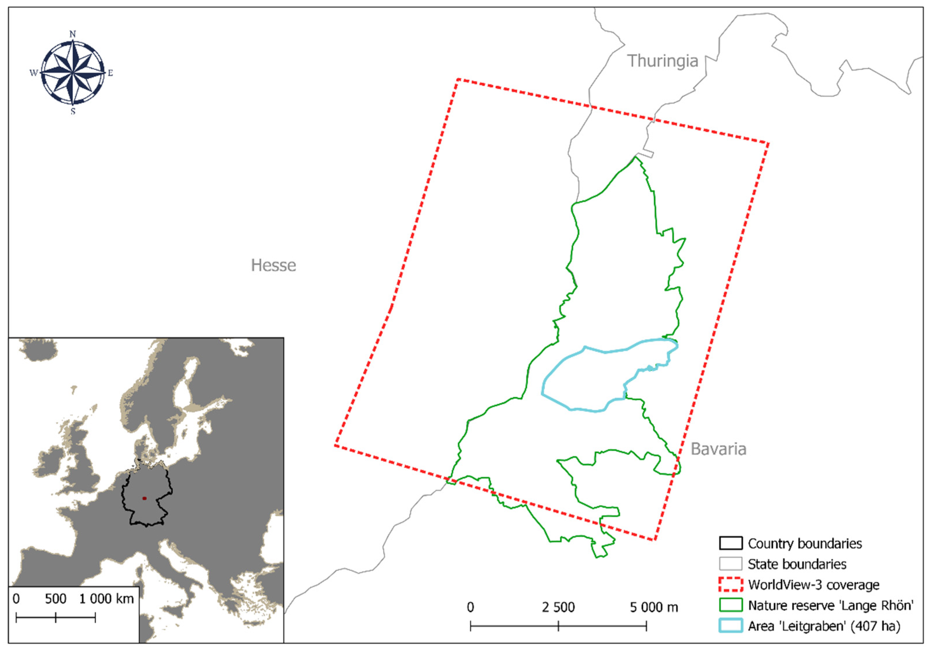
The Rhön UNESCO Biosphere Reserve is a 243.323 ha wide mountain region in central Germany in 600 to 950 m a.s.l. (Figure 1). Its core zone is characterized by extensively managed grasslands, mainly used as meadows and pastures. This special landscape provides a habitat for multiple endangered plant and animal species. The management strategy of large parts of the grasslands was optimized for the breeding behavior of Lyrurus tetrix. Therefore, these meadows were not mown in the early summer, which, among other things, supported the spread of L. polyphyllus in the region.
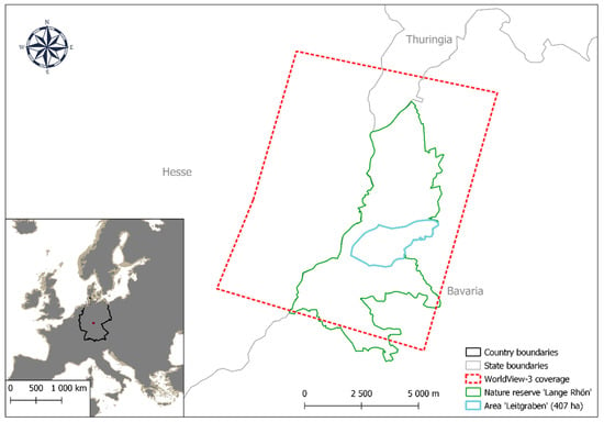
Figure 1.
Study area in nature reserve ‘lange Rhön’ in central Germany. Dotted red boundary represents WorldView-3 coverage used for training and testing. Blue boundary shows area ‘Leitgraben’ which was selected for the final prediction map.
L. polyphyllus was introduced to this area in the 1930s, as a soil cover for spruce plantations and to stabilize verges [27]. Due to the abandonment of the non-profitable meadows, L. Polyphyllus also spread in these grasslands, and from the mid-1990s, monitoring and management efforts have been carried out to control the species. Between 1996 and 2016, in parts of the Rhön UNESCO Biosphere Reserve (‘Leitgraben’), the spread of L. polyphyllus has doubled in terms of ground cover, both in open grassland areas as well as in areas which are difficult to manage, such as the margins of roads and near cairns build from stones removed from the grassland by farmers [21].
Its dominant stands have changed the habitat in such a way that ground breeding birds (e.g., Lyrurus tetrix and Crex crex) have lost breeding refugium and others their food supply. At the same time, the dominance of L. polyphyllus reduced the floral biodiversity, because species with smaller habitus are disadvantaged against the tall growth of L. polyphyllus single stands and especially large patches. Additionally, L. polyphyllus can transport nutrients from deeper soil levels upwards to the nutrient poor upper levels. The plant’s ability to fix atmospheric N can lead to higher nitrogen pools, which can lead to modified edaphic conditions, resulting in a loss of biodiversity [28].
2.2. Overview
Therefore, an eight-band multispectral WorldView-3 satellite image was acquired, and multiple machine learning (ML) methods have been trained and tested on their ability to classify L. polyphyllus at different degrees of ground cover. ML approaches have shown good capabilities to classify invasive species [29,30]. Additional feature selection procedures proved successful to decrease model complexity and increase model performance [16,31].
2.3. Satellite Data Acquisition
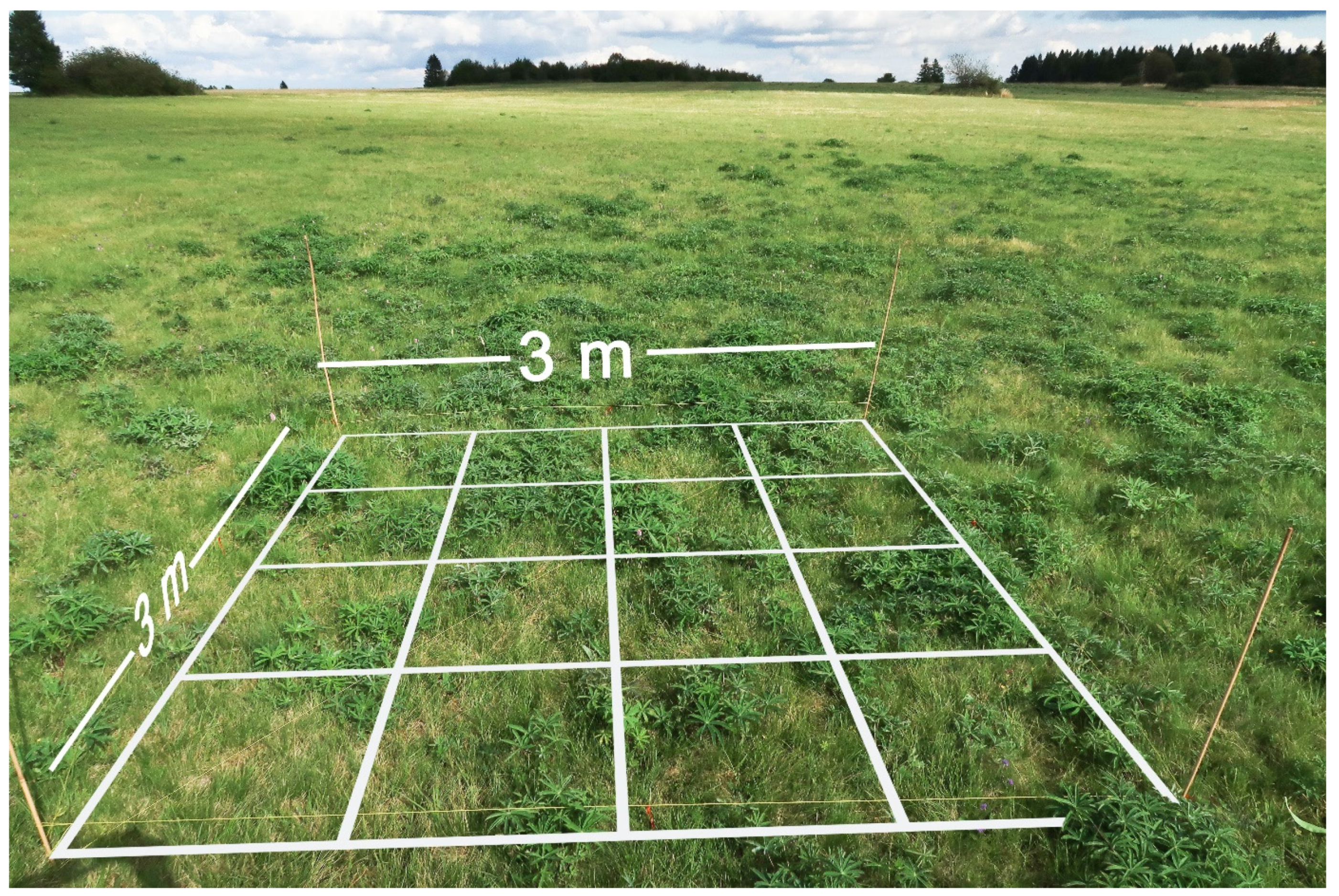
Satellite data was acquired from WorldView-3, a multi-payload, high-resolution satellite. It provides a spatial resolution of 31 cm for the panchromatic band, and 1.24 m for multispectral bands (Table 1). The image was taken on 6 August 2020 at 13:44 and covered a 100 km2 area along the core zone of the Rhön UNESCO Biosphere Reserve, where the ground sampling took place (~50°28′07.6′′ N and 10°02′03.8′′ E). Late summer was chosen for monitoring because at this time almost every meadow was mown, which commonly happens only once in the year, mostly in July. In August, L. polyphyllus has already regrown, while the surrounding grassland vegetation was still at almost cutting height (cf. Figure 2).

Table 1.
The bands of WorldView-3 used in this study. NIR: Near infrared.
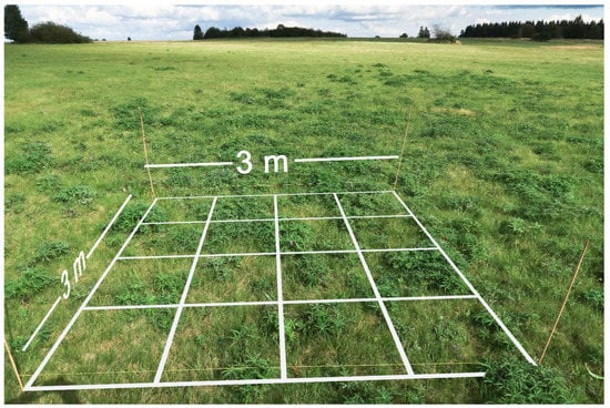
Figure 2.
Regrowth of L. polyphyllus after mowing on extensive grasslands at the Rhön UNESCO Biosphere Reserve in early September 2020.
2.4. Reference Ground Sampling
From 1st to 4th of September 2020, ground truth data were collected in the study area. Therefore, 3 × 3 m2 flexible frames were used (Figure 2), which have been divided into 16 equal squares (4 × 4 matrix with 0.75 m length). These frames were randomly distributed within the grasslands with a different ground cover of L. polyphyllus. For each sample, it was assessed how many of the 16 equal squares were at least partly covered with L. polyphyllus plants. A total of 219 3 × 3 m2 ground truth plots were set up for RS data analysis visually by experts in the field with different degrees of lupine contribution (Lupine cover classes from 0–16 which equals 0–100% with 6.25% cover steps). Each sample plot was documented with an RGB handheld camera image, taken from one side of the plot at a ca. 2 m distance. All four corners of each plot were measured with an RTK GNSS with a horizontal accuracy of 2 cm [32].
2.5. Pre-Processing of Satellite Data
Pre-processing steps were done in QGIS (v. 3.14.16). Calculations of TOAradiance (Equation (1)) and TOAreflectance (Equation (2)) (TOA: top of atmosphere) were made with the inbuild field calculator. Information on satellite and flight-specific parameters was given by the satellite data provider.
- 𝐿λ = Top of atmosphere radiance (spectral radiance at sensor) [W m−2 μm−1 sr−1)]
- 𝑔𝑎𝑖𝑛λ = Band-specific scaling factor [(W m−2 μm−1 sr−1)/DN]
- 𝐷𝑁λ = calibrated pixel value [DN]
- 𝑏𝑖𝑎𝑠λ = (upscaling factor/effective bandwidth) + OFFSET [W m−2 μm−1 sr−1]
- 𝜌𝜆 = Top of atmosphere reflectance (spectral reflectance at sensor) [unitless]
- 𝑑 = Distance Earth-Sun [au]
- 𝐸𝑒𝑥𝑜 = Exo-atmospheric radiance [W m−2 μm−1]
- 𝜃 = Solar zenith angle [°]
After these radiometric corrections, georeferencing was accomplished with coordinates collected with RTK GNSS (Leica Geosystems GmbH, Germany) at distinctive points (such as road marks and crossroads) in the study area.
2.6. Feature Creation
The panchromatic band and all eight spectral bands were used as features themself, as well as the Normalised Difference Spectral Indices (NDSI) calculated for each combination of multispectral bands (Equation (3)), resulting in additional 28 indices. Further, Haralick texture features [33] were calculated for panchromatic and multispectral bands with HaralickTextureExtraction plugin of Orfeo Toolbox library (OTB, open-source [34]) accessed from QGIS. Simple texture set selection was chosen as shown in Table 2, and image minimum and image maximum were adjusted for each band separately, depending on band intensity values. Expert knowledge was used to manually select all other preferences (computation step, radius, offset, histogram number of bins) to fit the purpose of generating distinguishable texture features (Table A1, Appendix A).

Table 2.
Haralick texture features computed over sliding windows with user defined radius. g(i,j) is the element in cell i, j of a normalized Grey Level Co-occurrence Matrix (GLCM).
- R = Spectral reflectance
- i = Wavelength [nm]
- j = Wavelength [nm]
From reference ground samples, plot corner coordinates were used to cut out each reference plot for each feature raster. As multiple pixels were located in a raster cut out, different metrics (average, standard deviation, minimum, maximum, 25% percentile, 50% percentile, 75% percentile) were used to calculate a value for each feature. In total, 763 features were created.
2.7. Feature Selection
To gain a higher model simplicity the total set of 763 features was reduced using the function VSURF (Variable Selection Using Random Forest) from R-package VSURF [37]. This method was chosen because it proved suitable both for binary outcomes (which was one of our classification scenarios—cf. Figure 3) and for datasets with many predictors [38]. In the first (thresholding) step of VSURF, irrelevant features were eliminated. A random forest with 50 runs was used to rank all features according to their importance measure (gain). A threshold was computed depending on the standard deviation of feature importance since irrelevant features have smaller standard deviations compared to features with high importance. The second (‘interpretation’) step reduced the feature set in nested random forest models (25 runs), starting with only the most important feature and finally selecting the feature set from the model with an out-of-bag error smaller than the minimal out-of-bag error augmented by its standard deviation. Selection from this step still contains features with redundancy for interpretation purposes. The third (‘prediction’) step was a forward selection procedure based on the previously selected feature set. Here, an additional feature was only added if the out-of-bag error significantly decreased compared to the average variation obtained by adding a noise feature [37].
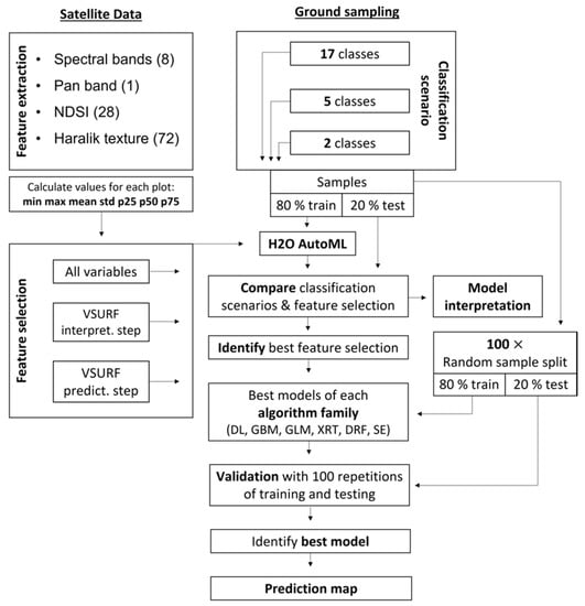
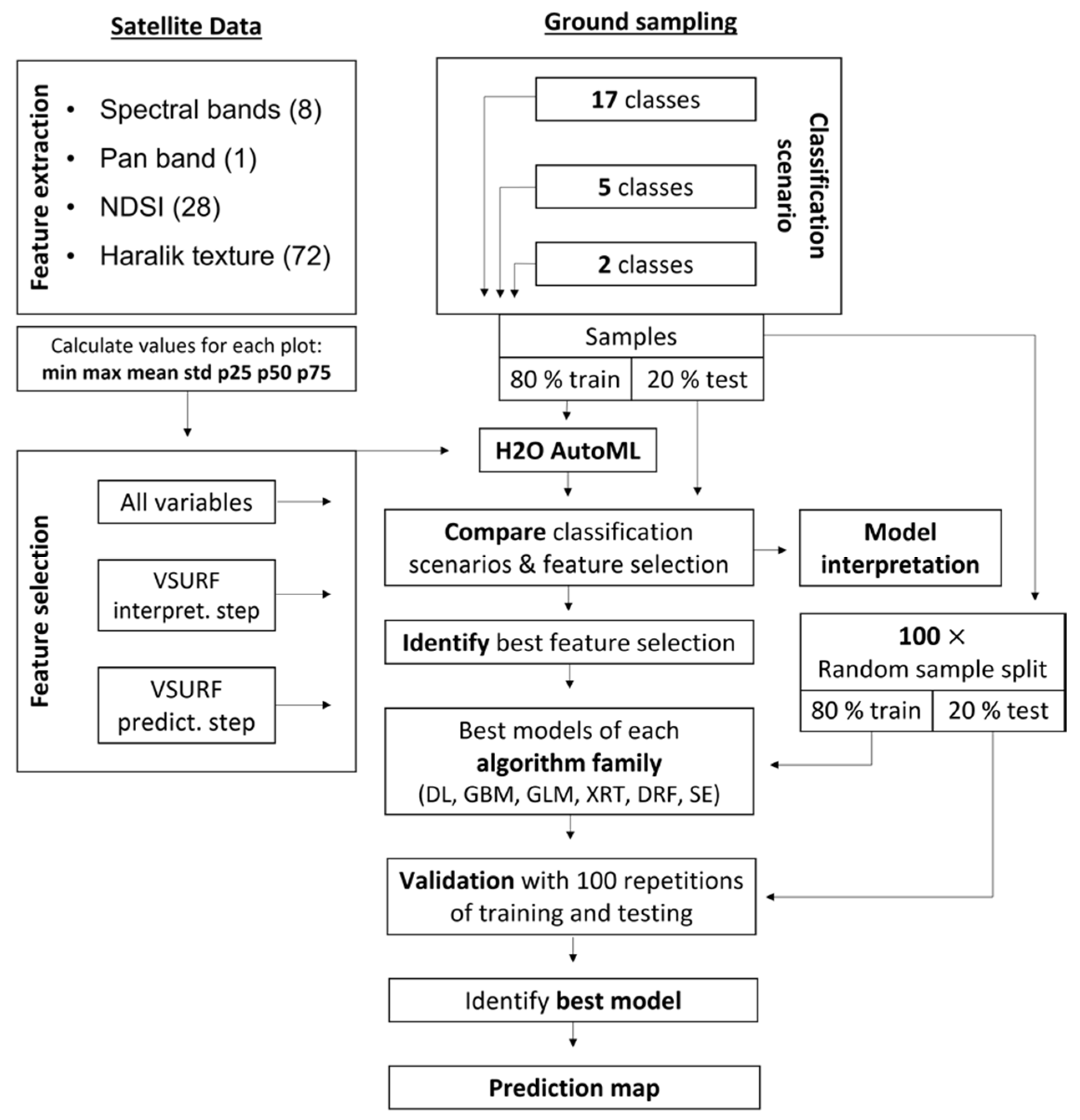
Figure 3.
Scheme of model development. DL: Deep Learning, GBM: Gradient Boosting Machine, GLM: Generalised Linear Model, XRT: Extremely Randomized Trees, DRF: Distributed Random Forest, SE: Stacken Ensembles.
2.8. Model Development
For model development, three different feature sets were used. The set with all 763 features, the one obtained by the VSURF ‘interpretation step’ and the one from VSURF ‘prediction step’. The sets were assigned to three different classification scenarios: A 17-class scenario, which included all documented data classes as described before (chap. 2.4. Reference ground sampling), a 5-class scenario, which aggregated the intermediate classes to nearly equal size in terms of the number of samples (cf. Figure A1), and a binary classification scenario which exclusively contained sample plots with 100% coverage of L. polyphyllus and those sample plots which were entirely free of L. polyphyllus. Therefore, the binary classification scenario only contained 82 of 219 samples.
Overall, 9 different modeling approaches were conducted (3 classification scenarios with three different feature sets each as input). Multiple machine learning algorithms were applied through the AutoML algorithm [39] from R-package H2O ([40] v. 3.32.0.4). H2O is a machine learning and predictive analysis platform that is written in Java and has an application programming interface that can be used by web interface, Phyton as well as R binding. AutoML can be used as an automatic machine learning workflow, including training and tuning of different supervised machine learning algorithms (DRF: Distributed Random Forest, XRT: Extremely Randomized Trees, GLM: Generalised Linear Model, GBM: Gradient Boosting Machine, deep learning, and stacked ensembles (cf. Table A2)). AutoML trains specific algorithms in the following order: A fixed grid of GLMs, a default DRF, five pre-specified GBMs, a near-default Deep Neural Net, an XRT, a random grid of GBMs, and a random grid of Deep Neural Nets. The number of models that are trained is eventually limited to a pre-defined training time. Additionally, and independent of time limitation, two stacked ensemble models are built, one (SEfamily) using only the best performing model of each algorithm family (DL, GBM, GLM, XRT, DRF) and one (SEall) combining all trained models.
Preferences of the AutoML function were kept similar for all classification scenarios and feature sets. Time limitation for the training process was limited to 600 s for each AutoML-run. A leader board, ranking all algorithms of a run depending on the mean per class error for multinominal classification and AUC (area under the receiver operating characteristic curve) for binary classification of a 5-fold cross-validation was created.
is the total number of observations of the corresponding data frame.
is the per observations user-defined weight (defaults is 1).
is the total number of classes (C = 2 for binary classification).
is the predicted value (uncalibrated probability) assigned to a given observation.
is the actual target value.
On a test dataset of 20% randomly picked samples, that represents a proportional split for each class, and which were not included in the training process, the validation measures mean per class error (Equations (4) and (5)) and Log loss (Equations (6) and (7)) were calculated and leaders inside each classification scenario were compared (all feature vs. VSURF ‘interpretation step’ vs. VSURF ‘prediction step’). Additionally, the best-performing algorithm was compared among the three different classification scenarios.
2.9. Model Interpretation
To get a better understanding of the underlying information of the prediction model, the contribution of each feature to the model was investigated. Feature importance was calculated for the best-performing model of the most promising AutoML run. Each algorithm family (DL, GBM, GLM, XRT, DRF) uses specific variable importance calculation (e.g., for deep learning it uses the Gedeon method [41]), which is executed with function h2o.varimp from the H2O package. The different calculation procedures are listed in the algorithm table (Table A2).
2.10. Final Validation of Best Model Approach
The best performing AutoML run (among all feature sets and classification scenarios) was inspected for its best models of each algorithm family (DL, GBM, GLM, XRT, DRF) and for the stacking ensemble model which was built by these five models. Each model was implemented in a loop of 100 training and testing steps, each built with a different combination of training and test samples. This was done to investigate the median prediction performance among all 100 runs to decrease the prediction outcome bias of a single test set that could be highly over-optimistic or over-pessimistic. Additionally, the range in prediction performance was used as an indicator for model stability. Median AUC (area under the ROC curve (receiver operating characteristic)) and median Log loss (Equations (6) and (7)) of each 100 model runs were compared to identify the best overall classification model for L. polyphyllus. Further, those median model’s ROC curves were compared to investigate their performance when the threshold for class probability is varied along the area of conflict between a high true positive rate (Equation (8)) and a low false positive rate (Equation (9)).
2.11. Binarization Threshold
Classifications with different binarization thresholds were performed additionally with the best performing AutoML algorithm. Therefore, samples were divided into binary classes by a threshold of L. polyphyllus coverage. As the sampling plots have been divided into 16 subplots, the same number of threshold values could be realized (in steps of 6.25% L. polyphyllus coverage). Classification performance was compared in terms of mean AUC after a loop of 100 training and testing steps, as described in the previous validation procedure. The threshold of the best performing model was identified to assess the minimum L. polyphyllus coverage necessary for ML-based identification of L. polyphyllus in practice.
2.12. Prediction Map
At last, the whole reference dataset was used as training input in the model with tuning parameters set according to the best performing model from AutoML run (Table A3) to create a prediction map of L. polyphyllus abundance for the target zone ‘Leitgraben’. To this end, the ‘h2o.predict’ function was used for calculating class probabilities (for classification), which can be labeled by a threshold that fits best the purpose of the prediction. Because missing a Lupine spot is much worse than a false alarm, the threshold that defines where to split the probabilistic classification value for assigning a predicted sample to a class should be oriented at a low false negative rate (Equation (10)). One way is to add a factor to the F1-score (Equation (12)), which is the harmonic mean of precision (Equation (11)) and recall (Equation (8)). The weighted F2-score (Equation (13)) penalizes more for false negative than false positive by adding a positive factor of 2 to the importance of recall, while the F0.5-score (Equation (14)) gives more weight to precision than to recall.
For this purpose, we identified the threshold value that gives a maximum performance of F0.5-score and F2-score to compare their outcome of L. polyphyllus prediction maps.
3. Results
3.1. AutoML Model Comparison
AutoML was used to compare the three different classification scenarios and to identify the most promising VSURF feature selection set. Among all nine AutoML runs, the 2-class scenario with VSURF ‘interpretation step’ as well as VSURF ‘prediction step’ feature set resulted in a gradient boosting machine algorithm as the leader model. All other leaders were deep learning algorithms. The overall best performing AutoML run was the binary GBM prediction model of Lupin vs. no-Lupin plots from VSURF ‘interpretation-step’ features. The mean per class error of 0.31 showed the second-lowest classification error after the 2-class scenario with all features but with a log loss of 0.75 the highest confidence in class assignment. In the 5-class scenario, the best leader model was a deep learning model built from VSURF ‘prediction step’. However, the mean per class error, as well as log loss, increased to 0.74 and 10.02 respectively. The leader from 17-class scenario performed worst (Table 3).

Table 3.
Leaders of all AutoML model runs validated on an external 20% test data set. Grey row shows the overall best model from all classification scenarios and feature sets.
3.2. Best AutoML Model
From all nine AutoML approaches Gradient Boosting Machine in combination with binary classification scenario with seven features performed most promising, resulting in a relatively low mean per class error along with a low Log loss. The confusion matrix (on 20% external test set) revealed a higher class error in the reference ‘Not Lupin’ class compared to reference ‘Lupin’ class (Table 4). The best model was built from a GBM with tuning parameters, as shown in Table A3.

Table 4.
Confusion Matrix of best model (GBM: Gradient Boosting Machine) from binary classification with 7 variables on external 20% test data set. UA: User Accuracy, PA: Producer Accuracy.
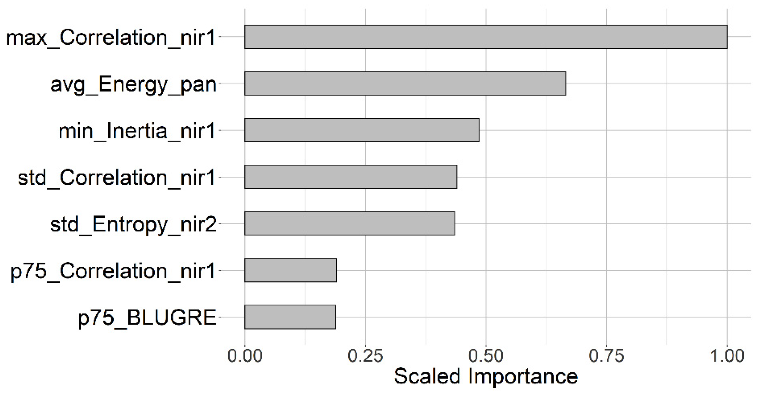
For the best model, the feature set was reduced to six Haralick texture features and one NDSI (p75_BLUGRE) calculated from the blue and green band. GBM variable importance, defined as the difference in squared error before and after a split using a particular feature, ranked all Haralick texture features before the NDSI feature (Figure 4).
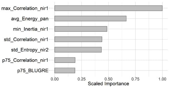
Figure 4.
Scaled feature importance of best (GBM) binary classification model. Importance is calculated as difference in squared error before and after a split using a particular feature. Variable p75_BLUGRE is the 75% percentile of the NDSI (Normalised Difference Spectral Index) calculated from Blue and Green band.
3.3. Validation with 100 Repetitions
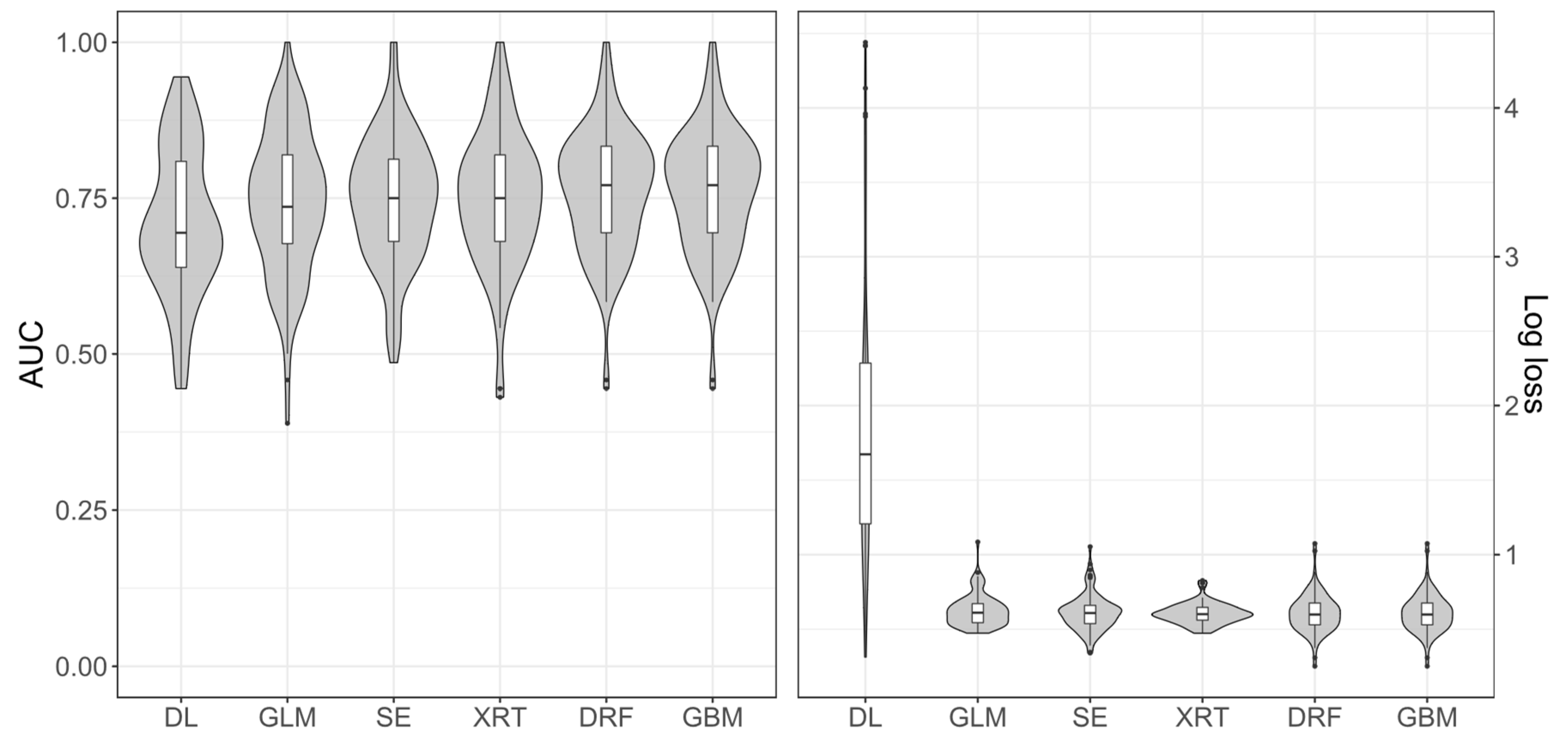
After the best AutoML run was identified, tuning parameters of the best models of each algorithm family were extracted from AutoML run to set up an additional validation step. Each model was trained and tested 100 times. Median AUC and Log loss for each algorithm was compared. GBM, the best model from AutoML run was among the other algorithms with a median AUC of 0.77. Median AUC and Log loss were generally similar for all algorithms, only DL with a high variation in Log loss and a lower median AUC, performed worse. XRT achieved the lowest variation in log loss values (Figure 5).
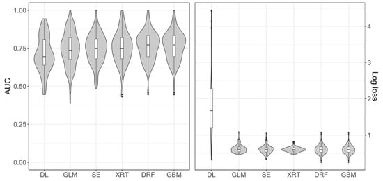
Figure 5.
Validation of 100 model run for the best models of each algorithm family from AutoML run based on 2-class scenario and VSURF ‘interpretation step’ feature set. Ordered by inreasing median ‘AUC’ (left) and decreasing median Log loss (right). DL: Deep Learning, DRF: Distributed Random Forest, GBM: Gradient Boosting Machine, XRT: Extremely Randomized Trees, GLM: Generalised Linear Model, SE: Stacken Ensembles.
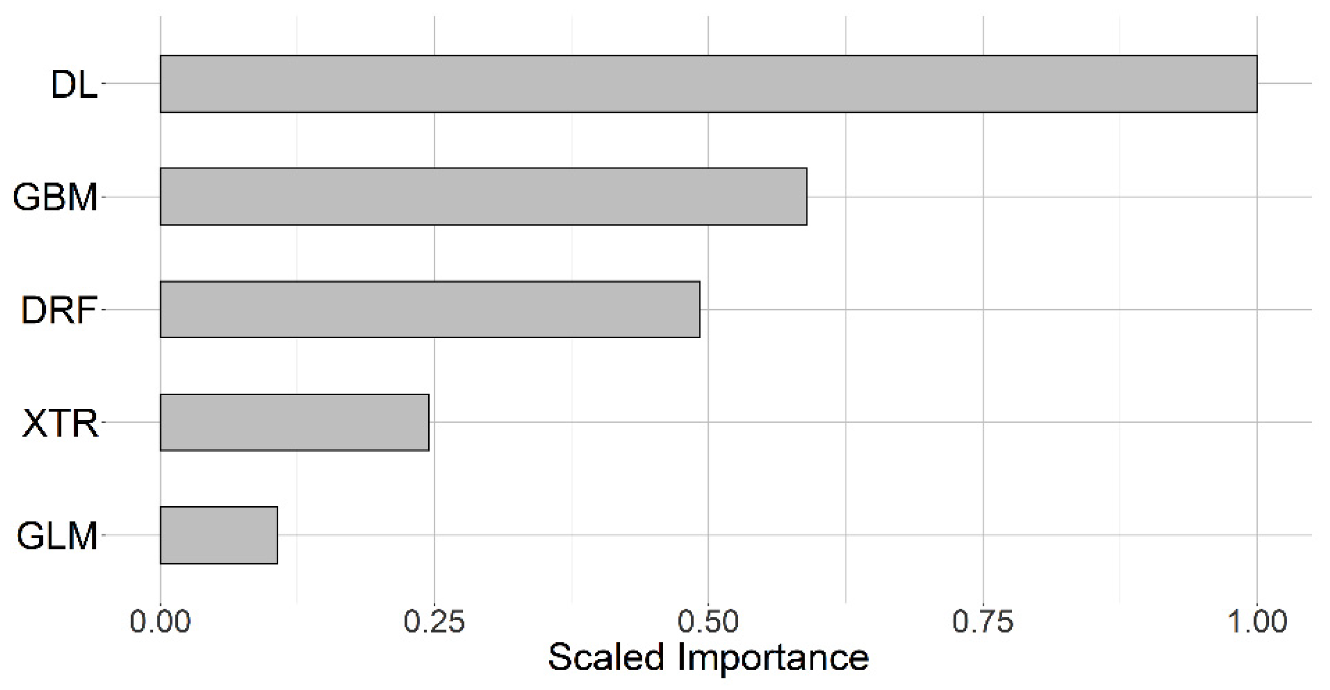
The SEfamily model was built from best-trained base learners (DRF, XRT, GLM, GBM, DL) for training a second-level “metalearner” based on a GLM algorithm. According to the feature importance of the metalearner, SEfamily model had the highest contribution from DL, followed by GBM, DRF, XRT, and GLM (Figure 6). The importance ranking is based on a standardized coefficient, which is the predictor weight of the standardized data.
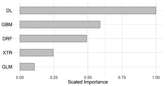
Figure 6.
Contribution of base learners to SEfamily built with GLM meta-learner and scaled importance between 0 and 1. The importance ranking is based on a standardized coefficient, which is the predictor weight of the standardized data. DL: Deep learning, DRF: Distributed Random Forest, GBM: Gradient Boosting Machine, GLM: Generalised Linear Model, SE: Stacked Ensembles, XRT: Extremely Randomized Trees.
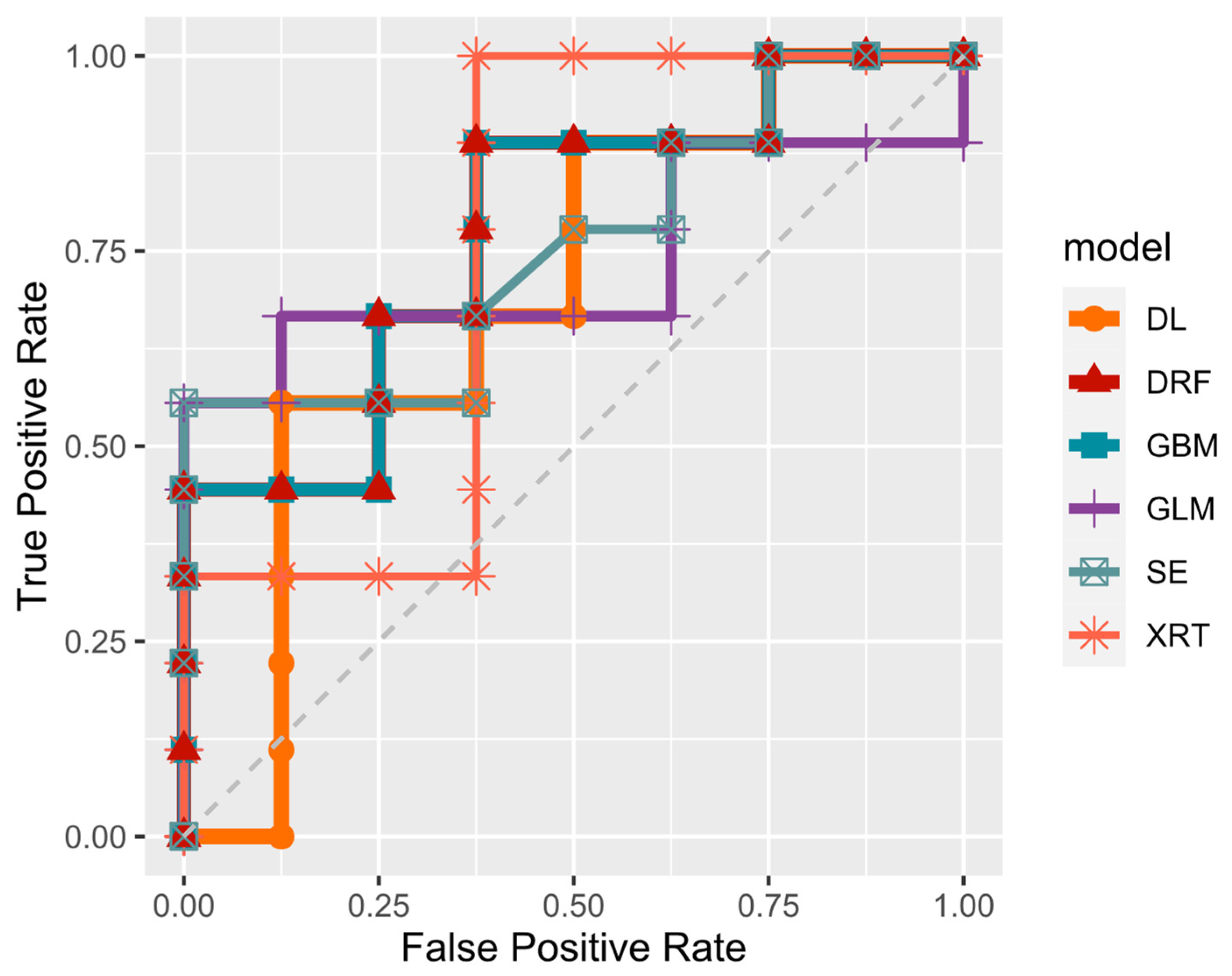
From 100 model runs within each algorithm family, the model with median AUC was used to illustrate ROC (receiver operating characteristic) curve. It showed that no algorithm was superior to others. SE and GLM were slightly superior at low false positive rates. A true positive rate (all Lupine samples detected) of 1 was achieved by the XRT model with a false positive rate (misclassified non-lupine samples) of 0.375 (Figure 7).
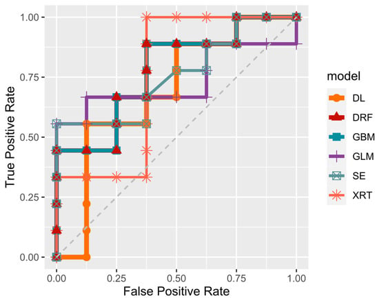
Figure 7.
ROC curve for median model from 100 model run of each algorithm family and a stacked ensemble build from these. DL: Deep learning, DRF: Distributed Random Forest, GBM: Gradient Boosting Machine, GLM: Generalized Linear Model, SE: Stacked Ensembles, XRT: Extremely Randomized Trees.
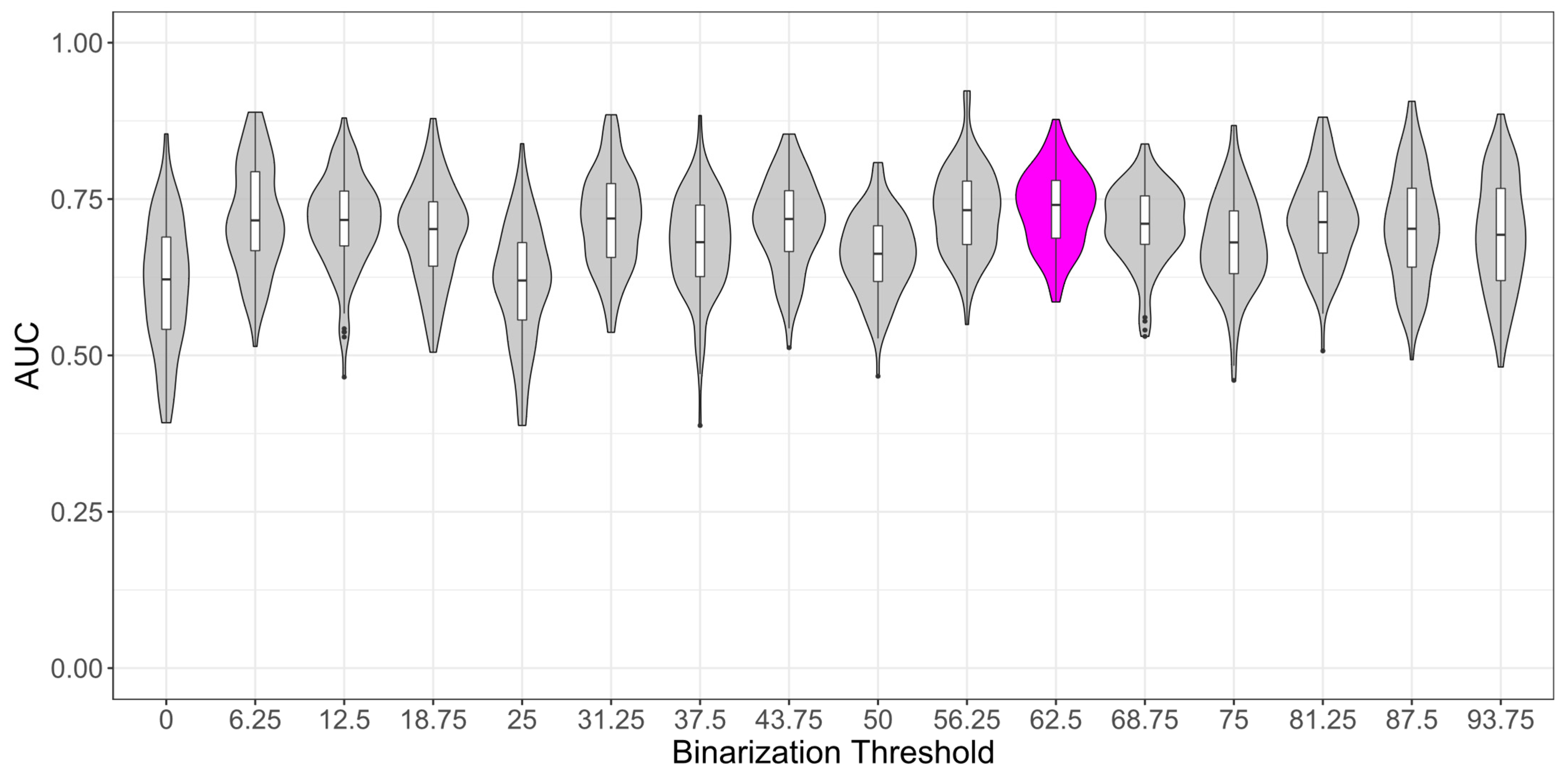
From 16 Binarization thresholds, a split at 62.5% L. polyphyllus coverage achieved the highest median AUC of 0.74 (Figure 8). All models performed worse compared to the binary model build only from samples with 0 and 100% L. polyphyllus coverage (cf. Figure 5). There was no clear trend in model performance along the threshold gradient of L. polyphyllus coverage.

Figure 8.
AUC from multiple binarization thresholds, dividing samples into classes according to their L. polyphyllus coverage. Highest mean AUC was achieved by the classification model that divided the two classes at 62.5% L. polyphyllus coverage. Boxplots represent AUC values from 100 model runs.
4. Discussion
4.1. Identifying the Most Promising Classification Algorithm Detecting L. polyphyllus Abundance from WorldView-3 Satellite Data
Our best binary classification showed slightly lower performance compared to other studies using WorldView-3 images to classify invasive plant species. [16] achieved accuracies between 76.6 and 91.2% with an XGBoost algorithm, depending on feature input (spectral and/or textural information), which is close to the accuracy of the GBM algorithm (from median AUC of 100 model runs) in the present study (77%).
It was expected that a stacked ensemble model would be top of the leader board, as a stack of complementary algorithms should increase the prediction performance compared to a single algorithm [42]. Instead, SEfamily model was on rank three after two GBM-based classifier variants (Figure A2). A single ML algorithm outperforming a stacked ensemble in remote sensing applications is not unusual and SE models should be built from carefully selected base classifiers [43]. Considering, that the SEfamily model was built from the best model of each algorithm family and that the most important algorithm inside the SEfamily was the DL model (Figure 6), which had the by far worst Log loss variation compared to all other algorithms in the 100-model run (Figure 5), the SEfamily model may have been limited by this and by a lower contribution of the outperforming GBM. Validation with 100 model runs revealed a high range in performance for all algorithms, which indicates a certain risk when dealing with a limited amount of sampling data. The goal should be to increase sampling size to further calibrate the prediction model.
As missing areas with L. polyphyllus abundance are worse than a false alarm, the threshold that defines were to split the probabilistic classification value for assigning a predicted sample to a class, should be oriented at a low missing rate. However, interpreting the results from the prediction map (Figure 9), the threshold for maximum F2-score is unfavorable, and a threshold from maximum F0.5-score seems more reasonable from expert knowledge of the invasion status of ‘Leitgraben’. This reveals the importance of ground truth knowledge and sensitivity for the decision of adequate thresholds of probabilistic classification models. Compared to the classification of invasive hogweed based on Pleiades 1B satellite data from [17], with a producer accuracy (PA) of 86% and a user accuracy (UA) of 94%, our GBM model (which had the highest median AUC) showed a somewhat higher PA of 89% and lower UA of 73%. Morphological differences between hogweed and L. polyphyllus, especially the plant and leaf size, could affect the performance of species identification. Further, the selection of samples for the non-target class is important as we have only chosen areas covered by grassland while [17] merged multiple different cover types to one ‘background’ cover class, increasing the difference between target and non-target class in terms of spectral and textural signatures. Hereby, we applied a less optimistic methodology that clearly reveals the challenges of identifying invasive species in ecosystems where invader and native vegetation show similarities in their spectral signatures and could thereby formulate the need for action in the development of RS-based large area species detection. Further, we could show that the final ML approach should be selected depending on the specific management aims. Therefore, ROC-curves seem appropriate to compare different ML approaches for operational tasks.

Figure 9.
Prediction map from the area ‘Leitgraben’ predicted by GBM with tuning parameters from the leader GBM model (Table A3). The threshold for class distribution was set to the maximum value of (a) F0.5-score and (b) F2-score.
4.2. Comparing Classification Performance with Different Numbers of Classes and Variable L. polyphyllus Cover
We could reveal the limitations of WorldView-3 multispectral data as a proxy for the detection of L. polyphyllus deriving performance measures from prediction models trained and validated for different resolutions of L. polyphyllus abundance. The binary classification was the only potentially useful approach compared to 5-class and 17-class scenarios. L. polyphyllus patches are therefore only detectable by WorldView-3 image-based classification models when they cover at least a 3 × 3 m ground surface. This is critical, as for management strategies, solitarily growing Lupin stands have been identified as the most important drivers of L. polyphyllus spread and invasion into new areas [27]. To reduce the lack of spatial resolution, aerial imagery, fixed wing drones, or drones with long-lasting batteries, flying at higher altitudes around 100 m AGL could be used instead. This would increase the spatial resolution to roughly 1–10 cm, and besides pixel-based approaches, additional approaches like Object Based Image Analysis could be considered [22], especially when high-resolution RGB imagery is available. However, this may increase the working load significantly and may lead to conflicts with nature protection aims such as the prevention of disturbance of wildlife animals. The validation of multiple binary classifications with different binarization thresholds showed no clear trend at which degree of L. polyphyllus cover a classification is most promising.
4.3. Comparing Classification Performance with Different Feature Selection Steps as Model Input
VSURF feature selection excluded most of the spectral raw data as well as NDSIs, which is not in line with results by Shendryk et al. (2020) where NDSI and single spectral bands were the most important features. In their study, only one texture feature was of any importance (‘Inverse Difference’), which was not selected in our study. Nevertheless, multispectral sensor information cannot be underestimated, as for the important texture features, NIR1 and NIR2 were the underlying spectral bands. NIR and red bands were the origins for the most important texture feature both in satellite-based [44] and UAV-based studies [36]. This indicates that the generalization of our findings across different invasive species is limited, instead, individual models need to be calibrated on individual feature sets. To increase the classification performance, texture feature extraction from NIR bands could be tuned to overcome the lack of spatial resolution.
4.4. General Concerns
We have chosen August for data acquisition to have notable regrowth of L. polyphyllus, while the surrounding grassland vegetation was still at almost stubble height from the previous cut. Therefore, L. polyphyllus is distinguishable from grassland vegetation on aerial imagery at this time in the year. Due to the lower resolution of our satellite data, a preponed monitoring alternative could also increase the classification performance of our models. At the end of June, when mowing is still restricted by nature protection constraints, and L. polyphyllus is in full blossom, spectral signatures of L. polyphyllus could be complemented by the prominent violet flower spikes. However, training prediction models based on blossoming plants only may lead to models that may miss many plants, as the phenological stage of individual plants is not always synchronous. Furthermore, other species with the same blossom color (e.g., Geranium sylvaticum) may complicate the model training process. It has to be stated that the time gap between satellite data acquisition (6 August 2020) and collection of reference ground data (1–4 September 2020) may have contributed to the fuzziness of models. Lowering the delay between both data acquisitions is important to disprove a significant regrowth until the event of ground reference data collection. Utilizing UAV-based semi-automatic reference data acquisition for training spacious satellite images (upscaling) could be an additional add-on to save the time of fieldwork and to create much more reference data of invasive species with high accuracy [19]. Further, the combination of different sensor data e.g., hyperspectral and LiDAR data [45] or optical and ultrasonic data, which has proven its potential for grassland quality parameters [46,47], could lead to higher classification results. A compromise in spatial and spectral resolution could also be derived from airborne hyperspectral [18,45] data.
5. Conclusions
As binary classification was the only potentially usable approach compared to 5-class and 17-class scenarios, L. polyphyllus patches are only detectable by WorldView-3 data, when they cover at least 3 × 3 m2 ground surface. We have to consider WorldView-3 data as very limited to L. polyphyllus detection in the late summer season.
If UAV-based missions are impossible due to nature conservation restriction, a future aim could be to train a WorldView-3 based classification model using times series [48,49] or collecting data in early summer at the peak of L. polyphyllus blossoming phenological stage.
We could show limitations for satellite-based species-detection in highly heterogenous grassland ecosystems and conclude that further sensor data fusion is necessary to compensate for similarities between target species and background as well as limits of the satellite’s spatial resolution.
Applicability is a crucial aspect in grassland monitoring to serve on strategic, tactic, and operational levels. To live up to the high expectations of RS-based monitoring tools, continuous development of RS methods under field conditions is inevitable.
Author Contributions
Conceptualization, D.S.-B., M.W. and T.A.; methodology, D.S.-B., M.W. and T.A.; software, D.S.-B.; validation, D.S.-B., formal analysis, D.S.-B.; investigation, D.S.-B., M.W. and T.A.; resources, T.A.; data M.W.; writing—original draft preparation, D.S.-B.; writing—review and editing, M.W. and T.A.; visualization, D.S.-B.; supervision, M.W. and T.A.; project administration, M.W.; funding acquisition, M.W. and T.A. All authors have read and agreed to the published version of the manuscript.
Funding
This research was funded by German Federal Environmental Foundation (Deutsche Bundesstiftung Umwelt- DBU, grant number: 32886/01-33/2).
Acknowledgments
The authors would like to thank Andrea Gerke and Eva Wiegard for their help in the field data collection. We are also grateful to the government of Bavaria for permission to conduct our measurements in a nature conservation area.
Conflicts of Interest
The authors declare no conflict of interest.
Appendix A
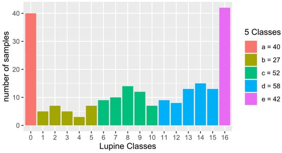
Figure A1.
Number of samples for each class. 2-class scenario only used class 0 and 16, while 17 class scenario used all classes. 5 class scenario divided samples as colour coded.
Figure A1.
Number of samples for each class. 2-class scenario only used class 0 and 16, while 17 class scenario used all classes. 5 class scenario divided samples as colour coded.

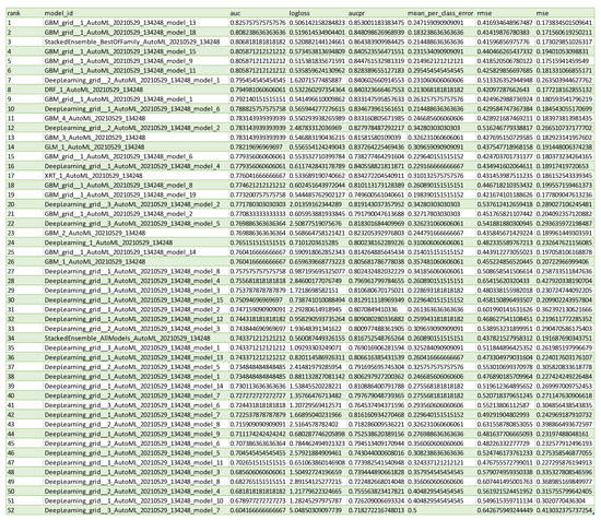
Figure A2.
Leader board from AutoML run with 2-classes and VSURF ‘interpretation step’ ranked by AUC of 5-fold cross validation.
Figure A2.
Leader board from AutoML run with 2-classes and VSURF ‘interpretation step’ ranked by AUC of 5-fold cross validation.
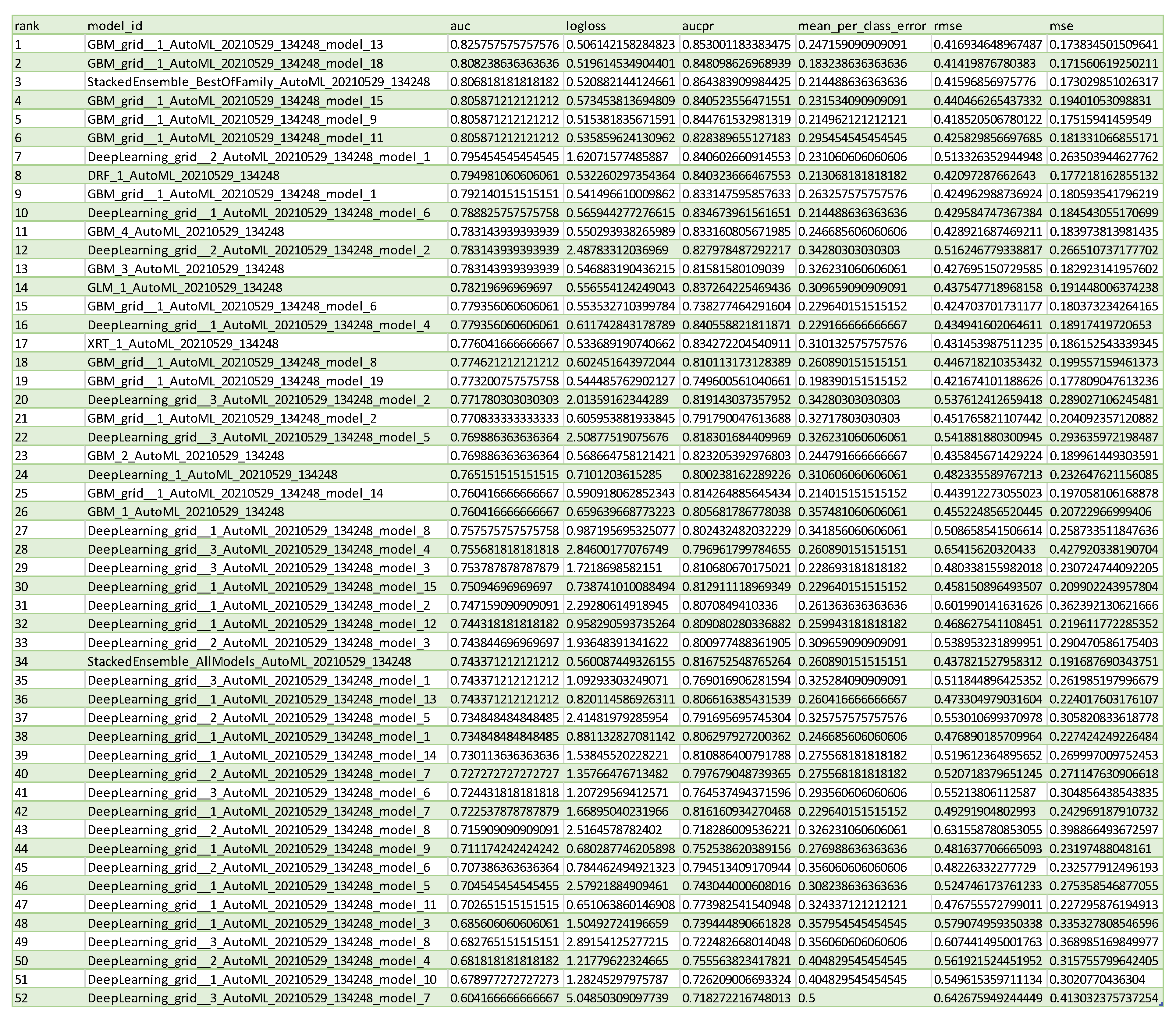

Table A1.
Haralick texture feature preferences.
Table A1.
Haralick texture feature preferences.
| Band | Computation Step | X Radius | Y Radius | X Offset | Y Offset | Image Minimum | Image Maximum | Histogram Number of Bins | Texture Set Selection |
|---|---|---|---|---|---|---|---|---|---|
| PAN | 1 | 2 | 2 | 1 | 1 | 100 | 362 | 32 | Simple |
| COASTAL | 1 | 2 | 2 | 1 | 1 | 0.09 | 0.131 | 256 | Simple |
| BLUE | 1 | 2 | 2 | 1 | 1 | 0.09 | 0.131 | 256 | simple |
| GREEN | 1 | 2 | 2 | 1 | 1 | 0.036 | 0.118 | 256 | simple |
| YELLOW | 1 | 2 | 2 | 1 | 1 | 0.025 | 0.118 | 256 | simple |
| RED | 1 | 2 | 2 | 1 | 1 | 0.018 | 0.135 | 256 | simple |
| REDEDGE | 1 | 2 | 2 | 1 | 1 | 0.024 | 0.27 | 256 | simple |
| NIR1 | 1 | 2 | 2 | 1 | 1 | 0.04 | 0.5 | 256 | simple |
| NIR2 | 1 | 2 | 2 | 1 | 1 | 0.03 | 0.42 | 256 | simple |

Table A2.
Machine Learning algorithms used by H20.
Table A2.
Machine Learning algorithms used by H20.
| Abbreviation | Name | Details | Feature Importance Calculation |
|---|---|---|---|
| DRF | Distributed Random Forest | Tree based algorithm with bagging [50]. Bagging has a parallel training stage for each learner. | Difference in squared error before and after a split using a particular feature. Improvements for a feature are summed up. |
| XRT | Extremely Randomized Trees | Same as DRF but with computed thresholds for tree splits. Reduced variance, increased bias [51]. | Difference in squared error before and after a split using a particular feature. Improvements for a feature are summed up. |
| GLM | Generalised Linear Model | For classification, GLM models the conditional class probability and uses a link function (logit for binomial) to relate the response variable to the generalize linear model [52].GLM uses elastic net regularization which is a combination of the ℓ1 and ℓ2 penalties to reduce overfitting. | Feature importance is the standardized coefficient, which is the predictor weight of the standardized data |
| GBM | Gradient Boosting | Tree based algorithm with boosting [53]. Boosting has a sequential training stage for each new learner, taking the previous classification success into account by increasing weight for misclassified data. | Difference in squared error before and after a split using a particular feature. Improvements for a feature are summed up. |
| DL | Deep learning | Multi-layer feedforward artificial neural network (multi-layer perceptron (MLP)) using back-propagation [54]. | Feature importance is calculated from Gedeon method [41] which uses a weight matrix analysis technique for determining the behavioural significance of hidden neurons. |
| SEfamily | Stacked ensembles from best model of each algorithm family | Trained base learners (best DRF, XRT, GLM, GBM, DL) are used for training a second level “metalearner” (with GLM). | Feature importance output is the contribution of each model to the stacked ensemble and not the underlying features from each base model itself. |
| SEall | Stacked ensembles from all models | Trained base learners (all DRF, XRT, GLM, GBM, DL) are used for training a second level “metalearner” (with GLM). | Feature importance output is the contribution of each model to the stacked ensemble and not the underlying features from each base model itself. |

Table A3.
Tuning parameters for GBM: Gradient Boosting Machine in AutoML run. Values of best GBM model are for 2-class scenario with VSURF ‘interpretation step’ feature set.
Table A3.
Tuning parameters for GBM: Gradient Boosting Machine in AutoML run. Values of best GBM model are for 2-class scenario with VSURF ‘interpretation step’ feature set.
| Paremeter | Searchable Values | Values of Best GBM Model |
|---|---|---|
| col_sample_rate | {0.4, 0.7, 1.0} | 0.4 |
| col_sample_rate_per_tree | {0.4, 0.7, 1.0} | 0.4 |
| learn_rate | Hard coded: 0.1 | 0.1 |
| max_depth | {3, 4, 5, 6, 7, 8, 9, 10, 11, 12, 13, 14, 15, 16, 17} | 13 |
| min_rows | {1, 5, 10, 15, 30, 100} | 5 |
| min_split_improvement | {1 × 10⁻⁴, 1 × 10⁻⁵} | 1 × 10⁻⁴ |
| ntrees | Hard coded: 10000 (true value found by early stopping) | 36 |
| sample_rate | {0.50, 0.60, 0.70, 0.80, 0.90, 1.00} | 1.00 |
References
- Wilson, J.B.; Peet, R.K.; Dengler, J.; Pärtel, M. Plant species richness: The world records. J. Veg. Sci. 2012, 23, 796–802. [Google Scholar] [CrossRef]
- Leadley, P.; Pereira, H.; Alkemade, R.; Alkemade, R.; JF, F.-M.; Proenca, V.; Scharlemann, J.; Walpole, M. Biodiversity Scenarios: Projections of 21st Century Change in Biodiversity and Associated Ecosystem Services; Secretariat of the Convention on Biological Diversity: Montreal, QC, Canada, 2010; Volume 50. [Google Scholar]
- De Bello, F.; Lavorel, S.; Díaz, S.; Harrington, R.; Cornelissen, J.H.C.; Bardgett, R.D.; Berg, M.P.; Cipriotti, P.; Feld, C.K.; Hering, D.; et al. Towards an assessment of multiple ecosystem processes and services via functional traits. Biodivers. Conserv. 2010, 19, 2873–2893. [Google Scholar] [CrossRef]
- Gross, J.; Woodley, S.; Welling, L.A.; Watson, J.E.M. Adapting to Climate Change: Guidance for Protected Area Managers and Planners. Best Practice Protected Area Guidelines Series No. 24; International Union for Conservation of Nature (IUCN): Gland, Switzerland, 2016. [Google Scholar]
- Seebens, H.; Blackburn, T.M.; Dyer, E.E.; Genovesi, P.; Hulme, P.E.; Jeschke, J.M.; Pagad, S.; Pyšek, P.; Winter, M.; Arianoutsou, M.; et al. No saturation in the accumulation of alien species worldwide. Nat. Commun. 2017, 8, 1–9. [Google Scholar] [CrossRef]
- Pejchar, L.; Mooney, H. The Impact of Invasive Alien Species on Ecosystem Services and Human Well-being. Bioinvasions Glob. Ecol. Econ. Manag. Policy 2010, 24. [Google Scholar] [CrossRef]
- Lambdon, P.W.; Pyšek, P.; Basnou, C.; Hejda, M.; Arianoutsou, M.; Essl, F.; Jarošík, V.; Pergl, J.; Winter, M.; Anastasiu, P.; et al. Alien flora of Europe: Species diversity, temporal trends, geographical patterns and research needs. Preslia 2008, 80, 101–149. [Google Scholar]
- Fremstad, E. NOBANIS—Invasive Alien Species Fact Sheet—Lupinus polyphyllus. Available online: /www.nobanis.org (accessed on 29 June 2021).
- Hejda, M.; Štajerová, K.; Pyšek, P. Dominance has a biogeographical component: Do plants tend to exert stronger impacts in their invaded rather than native range? J. Biogeogr. 2017, 44, 18–27. [Google Scholar] [CrossRef] [Green Version]
- Valtonen, A.; Jantunen, J.; Saarinen, K. Flora and lepidoptera fauna adversely affected by invasive Lupinus polyphyllus along road verges. Biol. Conserv. 2006, 133, 389–396. [Google Scholar] [CrossRef]
- Rehfuess, K.E.; Makeschin, F.; Rodenkirchen, H. Results and experience from amelioration trials in Scots pine (Pinus sylvestris L.) forests of Northeastern Bavaria. Fertil. Res. 1991, 27, 95–105. [Google Scholar] [CrossRef]
- Klinger, Y.P.; Hansen, W.; Otte, A.; Ludewig, K. Ausbreitungsvektoren und Ausbreitungswege der invasiven Stauden-Lupine im UNESCO Biosphärenreservat Rhön. BfN-Skripten 2019, 527, 167–172. [Google Scholar]
- Ludewig, K.; Hansen, W.; Klinger, Y.P.; Eckstein, R.L.; Otte, A. Seed bank offers potential for active restoration of mountain meadows. Restor. Ecol. 2021, 29, 1–9. [Google Scholar] [CrossRef]
- Lelong, C.C.D.; Tshingomba, U.K.; Soti, V. Assessing Worldview-3 multispectral imaging abilities to map the tree diversity in semi-arid parklands. Int. J. Appl. Earth Obs. Geoinf. 2020, 93, 102211. [Google Scholar] [CrossRef]
- Choudhury, M.A.M.; Marcheggiani, E.; Galli, A.; Modica, G.; Somers, B. Mapping the Urban Atmospheric Carbon Stock by LiDAR and WorldView-3 Data. Forests 2021, 12, 692. [Google Scholar] [CrossRef]
- Shendryk, Y.; Rossiter-Rachor, N.A.; Setterfield, S.A.; Levick, S.R. Leveraging High-Resolution Satellite Imagery and Gradient Boosting for Invasive Weed Mapping. IEEE J. Sel. Top. Appl. Earth Obs. Remote Sens. 2020, 13, 4443–4450. [Google Scholar] [CrossRef]
- Müllerová, J.; Brůna, J.; Bartaloš, T.; Dvořák, P.; Vítková, M.; Pyšek, P. Timing is important: Unmanned aircraft vs. Satellite imagery in plant invasion monitoring. Front. Plant Sci. 2017, 8, 1–13. [Google Scholar] [CrossRef] [PubMed] [Green Version]
- Skowronek, S.; Asner, G.P.; Feilhauer, H. Performance of one-class classifiers for invasive species mapping using airborne imaging spectroscopy. Ecol. Inform. 2017, 37, 66–76. [Google Scholar] [CrossRef]
- Kattenborn, T.; Lopatin, J.; Förster, M.; Braun, A.C.; Fassnacht, F.E. UAV data as alternative to field sampling to map woody invasive species based on combined Sentinel-1 and Sentinel-2 data. Remote Sens. Environ. 2019, 227, 61–73. [Google Scholar] [CrossRef]
- Jensen, T.; Hass, F.S.; Akbar, M.S.; Petersen, P.H.; Arsanjani, J.J. Employing machine learning for detection of invasive species using sentinel-2 and aviris data: The case of Kudzu in the United States. Sustainability 2020, 12, 3544. [Google Scholar] [CrossRef]
- Klinger, Y.P.; Harvolk-Schöning, S.; Eckstein, R.L.; Hansen, W.; Otte, A.; Ludewig, K. Applying landscape structure analysis to assess the spatio-temporal distribution of an invasive legume in the Rhön UNESCO Biosphere Reserve. Biol. Invasions 2019, 21, 2735–2749. [Google Scholar] [CrossRef]
- Wijesingha, J.; Astor, T.; Schulze-Brüninghoff, D.; Wachendorf, M. Mapping Invasive Lupinus polyphyllus Lindl. in Semi-natural Grasslands Using Object-Based Image Analysis of UAV-borne Images. PFG—J. Photogramm. Remote Sens. Geoinf. Sci. 2020, 88, 391–406. [Google Scholar] [CrossRef]
- Mulero-Pázmány, M.; Jenni-Eiermann, S.; Strebel, N.; Sattler, T.; Negro, J.J.; Tablado, Z. Unmanned aircraft systems as a new source of disturbance for wildlife: A systematic review. PLoS ONE 2017, 12, 1–14. [Google Scholar] [CrossRef] [Green Version]
- McEvoy, J.F.; Hall, G.P.; McDonald, P.G. Evaluation of unmanned aerial vehicle shape, flight path and camera type for waterfowl surveys: Disturbance effects and species recognition. PeerJ. 2016, 2016. [Google Scholar] [CrossRef] [Green Version]
- Lyons, M.; Brandis, K.; Callaghan, C.; McCann, J.; Mills, C.; Ryall, S.; Kingsford, R. Bird interactions with drones, from individuals to large colonies. bioRxiv 2017. [Google Scholar] [CrossRef] [Green Version]
- Israel, M.; Reinhard, A. Detecting nests of lapwing birds with the aid of a small unmanned aerial vehicle with thermal camera. In Proceedings of the 2017 International Conference on Unmanned Aircraft Systems (ICUAS), Miami, FL, USA, 13–16 June 2017; pp. 1199–1207. [Google Scholar] [CrossRef] [Green Version]
- Volz, H. Ursachen und Auswirkungen der Ausbreitung von Lupinus polyphyllus Lindl. im Bergwiesenökosystem der Rhön und Maßnahmen zu Seiner Regulierung; Justus-Liebig-Universität Gießen: Gießen, Germany, 2003. [Google Scholar]
- Hansen, W.; Wollny, J.; Otte, A.; Eckstein, R.L.; Ludewig, K. Invasive legume affects species and functional composition of mountain meadow plant communities. Biol. Invasions 2020, 23, 281–296. [Google Scholar] [CrossRef]
- James, K.; Bradshaw, K. Detecting plant species in the field with deep learning and drone technology. Methods Ecol. Evol. 2020, 11, 1509–1519. [Google Scholar] [CrossRef]
- Shiferaw, H.; Bewket, W.; Eckert, S. Performances of machine learning algorithms for mapping fractional cover of an invasive plant species in a dryland ecosystem. Ecol. Evol. 2019, 9, 2562–2574. [Google Scholar] [CrossRef] [Green Version]
- Demarchi, L.; Kania, A.; Ciezkowski, W.; Piórkowski, H.; Oświecimska-Piasko, Z.; Chormański, J. Recursive feature elimination and random forest classification of natura 2000 grasslands in lowland river valleys of poland based on airborne hyperspectral and LiDAR data fusion. Remote Sens. 2020, 12, 1842. [Google Scholar] [CrossRef]
- Leica Geosystems Leica ScanStation P30/P40; Leica Geosystems AG: Heerbrugg, Schweiz, 2017; Volume 2.
- Haralick, R.M.; Shanmugam, K.; Dinstein, I. Textural Features for Image Classification. IEEE Trans. Syst. Man. Cybern. 1973, SMC-3, 610–621. [Google Scholar] [CrossRef] [Green Version]
- Grizonnet, M.; Michel, J.; Poughon, V.; Inglada, J.; Savinaud, M.; Cresson, R. Orfeo ToolBox: Open source processing of remote sensing images. Open Geospat. Data Softw. Stand. 2017, 2, 1–8. [Google Scholar] [CrossRef] [Green Version]
- OTB Development Team. The Orfeo ToolBox Cookbook, a Guide for Non-Developers Updated for OTB-3.14. Available online: http://sossvr1.liberaintentio.com/otb/OTBCookBook.pdf (accessed on 29 June 2021).
- Grüner, E.; Wachendorf, M.; Astor, T. The potential of UAV-borne spectral and textural information for predicting aboveground biomass and N fixation in legume-grass mixtures. PLoS ONE 2020, 15, 1–21. [Google Scholar] [CrossRef] [PubMed]
- Genuer, R.; Poggi, J.-M.; Tuleau-Malot, C. VSURF: Variable Selection Using Random Forests. Available online: https://cran.r-project.org/package=VSURF (accessed on 29 June 2021).
- Speiser, J.L.; Miller, M.E.; Tooze, J.; Ip, E. A comparison of random forest variable selection methods for classification prediction modeling. Expert Syst. Appl. 2019, 134, 93–101. [Google Scholar] [CrossRef]
- LeDell, E.; Poirier, S. H2O AutoML: Scalable Automatic Machine Learning. In Proceedings of the 7th ICML Workshop on Automated Machine Learning, Vienna, Austria, 12–18 July 2020. [Google Scholar]
- H2O.ai R Interface for H2O. Available online: https://github.com/h2oai/h2o-3 (accessed on 29 June 2021).
- Gedeon, T.D. Data mining of inputs: Analysing magnitude and functional measures. Int. J. Neural Syst. 1997, 8, 209–218. [Google Scholar] [CrossRef] [PubMed]
- Fang, Z.; Wang, Y.; Peng, L.; Hong, H. A comparative study of heterogeneous ensemble-learning techniques for landslide susceptibility mapping. Int. J. Geogr. Inf. Sci. 2021, 35, 321–347. [Google Scholar] [CrossRef]
- Vasilakos, C.; Kavroudakis, D.; Georganta, A. Machine learning classification ensemble of multitemporal Sentinel-2 images: The case of a mixed mediterranean ecosystem. Remote Sens. 2020, 12, 2005. [Google Scholar] [CrossRef]
- Gallardo-Cruz, J.A.; Meave, J.A.; González, E.J.; Lebrija-Trejos, E.E.; Romero-Romero, M.A.; Pérez-García, E.A.; Gallardo-Cruz, R.; Hernández-Stefanoni, J.L.; Martorell, C. Predicting tropical dry forest successional attributes from space: Is the key hidden in image texture? PLoS ONE 2012, 7, 38–45. [Google Scholar] [CrossRef] [Green Version]
- Kopeć, D.; Sabat-Tomala, A.; Michalska-Hejduk, D.; Jarocińska, A.; Niedzielko, J. Application of airborne hyperspectral data for mapping of invasive alien Spiraea tomentosa L.: A serious threat to peat bog plant communities. Wetl. Ecol. Manag. 2020, 28, 357–373. [Google Scholar] [CrossRef] [Green Version]
- Moeckel, T.; Safari, H.; Reddersen, B.; Fricke, T.; Wachendorf, M. Fusion of ultrasonic and spectral sensor data for improving the estimation of biomass in grasslands with heterogeneous sward structure. Remote Sens. 2017, 9, 98. [Google Scholar] [CrossRef] [Green Version]
- Safari, H.; Fricke, T.; Reddersen, B.; Möckel, T.; Wachendorf, M. Comparing mobile and static assessment of biomass in heterogeneous grassland with a multi-sensor system. J. Sensors Sens. Syst. 2016, 5, 301–312. [Google Scholar] [CrossRef] [Green Version]
- Förster, M.; Schmidt, T.; Wolf, R.; Kleinschmit, B.; Fassnacht, F.E.; Cabezas, J.; Kattenborn, T. Detecting the spread of invasive species in central Chile with a Sentinel-2 time-series. In Proceedings of the 2017 9th International Workshop on the Analysis of Multitemporal Remote Sensing Images (MultiTemp), Bruges, Belgium, 27–29 June 2017; pp. 1–4. [Google Scholar]
- Somers, B.; Asner, G.P. Invasive Species Mapping in Hawaiian Rainforests Using Multi-Temporal Hyperion Spaceborne Imaging Spectroscopy. IEEE J. Sel. Top. Appl. Earth Obs. Remote Sens. 2013, 6, 351–359. [Google Scholar] [CrossRef] [Green Version]
- Breiman, L. Random Forests. Mach. Learn. 2001, 45, 5–32. [Google Scholar] [CrossRef] [Green Version]
- Geurts, P.; Ernst, D.; Wehenkel, L. Extremely randomized trees. Mach. Learn. 2006, 63, 3–42. [Google Scholar] [CrossRef] [Green Version]
- Nelder, J.A.; Wedderburn, R.W.M. Generalized Linear Models. J. R. Stat. Soc. Ser. A 1972, 135, 370–384. [Google Scholar] [CrossRef]
- Friedman, J.H. Greedy function approximation: A gradient boosting machine. Ann. Stat. 2001, 29, 1189–1232. [Google Scholar] [CrossRef]
- LeCun, Y.; Bengio, Y.; Hinton, G. Deep learning. Nature 2015, 521, 436–444. [Google Scholar] [CrossRef] [PubMed]
Publisher’s Note: MDPI stays neutral with regard to jurisdictional claims in published maps and institutional affiliations. |
© 2021 by the authors. Licensee MDPI, Basel, Switzerland. This article is an open access article distributed under the terms and conditions of the Creative Commons Attribution (CC BY) license (https://creativecommons.org/licenses/by/4.0/).

