Article

Prediction of Forest Fire Spread Rate Using UAV Images and an LSTM Model Considering the Interaction between Fire and Wind

1
College of Mechanical and Electrical Engineering, Northeast Forestry University, Harbin 150040, China
2
Northern Forest Fire Management Key Laboratory of the State Forestry and Grassland Bureau, Northeast Forest University, Harbin 150040, China
3
College of Engineering and Technology, Northeast Forestry University, Harbin 150040, China
4
College of Forestry, Northeast Forestry University, Harbin 150040, China
*
Author to whom correspondence should be addressed.
Remote Sens. 2021, 13(21), 4325; https://doi.org/10.3390/rs13214325
Submission received: 9 September 2021 / Revised: 17 October 2021 / Accepted: 24 October 2021 / Published: 27 October 2021
(This article belongs to the Special Issue Remote Sensing and Smart Forestry)

Abstract

:
Modeling forest fire spread is a very complex problem, and the existing models usually need some input parameters which are hard to get. How to predict the time series of forest fire spread rate based on passed series may be a key problem to break through the current technical bottleneck. In the process of forest fire spreading, spread rate and wind speed would affect each other. In this paper, three kinds of network models based on Long Short-Term Memory (LSTM) are designed to predict fire spread rate, exploring the interaction between fire and wind. In order to train these LSTM-based models and validate their effectiveness of prediction, several outdoor combustion experiments are designed and carried out. Process data sets of forest fire spreading are collected with an infrared camera mounted on a UAV, and wind data sets are recorded using a anemometer simultaneously. According to the close relationship between wind and fire, three progressive LSTM based models are constructed, which are called CSG-LSTM, MDG-LSTM and FNU-LSTM, respectively. A Cross-Entropy Loss equation is employed to measure the model training quality, and then prediction accuracy is computed and analyzed by comparing with the true fire spread rate and wind speed. According to the performance of training and prediction stage, FNU-LSTM is determined as the best model for the general case. The advantage of FNU-LSTM is further demonstrated by doing comparison experiments with the normal LSTM and other LSTM based models which predict both fire spread rate and wind speed separately. The experiment has also demonstrated the ability of the model to the real fire prediction on the basis of two historical wildland fires.

1. Introduction

Forest fire is one of the major natural disasters, and it occurred frequently in the last few years [1]. For example, in 2020, the super fire of Australia lasted for about half of year, which killed 33 persons, and the burned area exceeded 10 million hectares, causing great damage to the local ecosystem. In April 2019, a forest fire broke out in Liangshui, Sichuan, China. Due to the neglect of the impact of factors such as the terrain environment and the abrupt change of wind direction during the spread of the forest fire, a deflagration fire occurred, resulting in the sacrifice of 27 forest firefighters, as well as irreparable social and economic losses. The spread and development of forest fires are affected by the topographic environment, and the spread of forest fire also affects local forest weather environment. Therefore, the mutual influence between forest fire spread and local environmental factors cannot be ignored for prevention and control of forest fire spread.
It is a very complicated task to completely simulate the various combustion state parameters of a real forest fire. Some scholars have proposed the fire identification algorithms, which provide technical support for fire prediction. The fire identification algorithm is designed based on computer vision [2]. The detection system based on the TDLAS is designed; it can find fires by measuring the concentrations of CO [3]. Because the actual environment is complex, it is often difficult to accurately measure the external environmental factors that affect the spread of the forest fire, such as wind speed and water content, types of combustibles, temperature and humidity, etc. Therefore, most of the simulation and prediction work at this stage is based on laboratory conditions to derive the propagation speed formula under certain conditions, and then it is generalized to the corresponding real environment. Based on physics and statistical experience, some classic forest fire models such as Albini model [4], Australian Mcarthur model [5], Canadian forest fire model [6], Rothermel model [7,8] and Wang Zhengfei model [9] are proposed.
These theoretical models fully demonstrate the relationship between the spread of forest fires and the characteristics of combustibles and environmental factors on the basis of a large number of forest fire experiments, and quantify their use of mathematical relationships to reflect their mutual effects. Based on these theories, cellular automata [10,11], boundary interpolation [12,13] and maze algorithm [14,15] or other computational simulation algorithms are used to describe the process of forest fire spread in the form of grid or vector graphics. Zeng [16] uses big data analysis technology to conduct forest fire dynamic prediction. In response to the sudden changing characteristics of forest fire behavior, Zhou [17] combined a dynamic data system and discrete event system specification model, and proposed a dynamic data-driven forest fire spread model based on DEVS modeling [18]. Because the external environmental factors and the internal characteristics of combustibles cannot be reflected by qualitative mathematical formulas, this theoretical model is not necessarily suitable for complex forest wildfire combustion sites.
Wind speed is one of the most important factors affecting the spread of forest fires, and many scholars have conducted research on its forecasting methods. He [19] proposed a hybrid forecasting system. In this system, the decomposition technology is applied to reduce the influence of noise in the original data sequence to obtain a more stable sequence. Chen [20] contributes to the development of an effective multistep forecasting method termed ECKIE, which provides multistep forecast for the very-short-term wind speed in specific stations. The developed method is capable of clustering the model inputs into groups according to their characteristics and reducing forecasting errors by choosing a suitable model. Li [21] proposed a self-adaptive kernel extreme learning machine (KELM) with an advanced and efficient learning process, the self-adaptive KELM could simultaneously make old data obsolete while learning from new data by reserving overlapped information between the updated and old training datasets.
Some other novel algorithms [22] on deep learning provide a very good approach to tackling the fire spread modeling problems. LSTM [23,24,25,26,27,28] has strong nonlinear fitting ability, simple learning rules and does not have the problem of excessive expansion of parameters when facing large data sets. For example, in the field of motion capture with strong timeliness, the TMF-LSTM [29] network, an extended network of LSTM, can well capture the co-occurrence relationship between time and space. In the network, the LSTM approach predicts the topology of the next network, respecting the local network topology and the dynamics of the network in the short term. The results of the experiment prove that the significant advantages of the proposed model compared to other strong competitors. A conditional generative adversarial network with long short-term memory structure (LSTM-CGAN) [30] has also made great achievements in the field of space-time monitoring. The author uses taxi hotspot data to train LSTM-CGAN, and the results show that the proposed LSMT-CGAN model is superior to all the benchmark methods and shows great potential to make many shared mobile applications.
LSTM not only applies to the related fields of human action, but also has a good effect on the learning of natural environment factors. T. Vinothkumar [31] proposed a recurrent neural network model called the LSTM network model, and variants of support vector machine models are used to predict the wind speed for the considered locations where the windmill has been installed, so that it results in forecasting the possible wind power that can be generated from the wind resources which facilitates to meet the growing energy demand. Pan [32] constructed a CNN-GRU model to predict the water level of the Yangtze River. It is proved that the accuracy of the model is higher than that of the autoregressive integrated moving average model (ARIMA) [33] and wavelet-based artificial neural network (WANN) [34] from three aspects: Nash–Sutcliffe efficiency coefficient (NSE) [35], average relative error (MRE) [36] and root mean square error (RMSE) [37]. From the above examples, it can be seen that LSTM network can well capture the characteristics of complex time series and solve the problem of long-term dependence.
The prediction of forest fire spread is a complicated time series problem. The traditional mathematical theory model usually obtains the fire spread rate model by controlling the properties of combustibles and the parameters of the external environment under the laboratory conditions. This means that traditional theoretical models have great limitations in practical application because parameters such as combustible properties are often difficult to obtain in the combustion zone. Therefore, this paper will use LSTM to design a new neural network model to predict the spread rate of the forest fire. In order to deeply capture the characteristics of forest fire spread by the neural network, we choose the external parameters that have key impact to the process of forest fire spread as the input parameters to assist the neural network in learning the rate of fire spread. By studying the theoretical models related to forest fire spread, such as the Rothermel model, Wang Zhengfei model, various subsequent improved models, etc., we can see that terrain and wind speed are two important parameters that affect forest fire spread. When a forest fire erupts in a specific scene, the terrain characteristics are often fixed, and there will not be much change during the forest fire spreading process.
The scientific hypothesis of the work is that fire and wind interact with each other, and that wind speed and fire speed are related in terms of the time series. Therefore, the research in this paper focuses on exploring the relationship between wind speed and forest fire spreading rate. Although the temperature and relative humidity of the air can influence forest fire spread, we study the time series evolution problem for fire and wind. Wind is the key element for fire spreading, and fire meteorology can also generate the change of wind, so it is of great significance to predict both fire and wind simultaneously on the basis that other influencing elements are stable. We believe forest fire spread speed can be predicted more accurately if the wind speed is considered in the prediction model. Extreme fire behavior is often caused by the interaction between fire and wind, and the application of the model in the forest fire management can reduce the casualties due to the extreme fire.
The main characteristics of the work include the following three points. First, in order to make the LSTM neural network be able to perceive the changes of the external environment while learning the fire spread rate, we introduced the progressive structure into the network unit to make the model have good real time performance. Second, we need to learn not only fire spread rate, but also wind speed. The accurate prediction of wind speed can also improve LSTM network to capture the time characteristics of fire spread rate. Finally, in order to fully verify the applicability of the model, we use outdoor burning data sets and wildland fire data sets to compare the model proposed in this paper with some excellent LSTM models involved in other papers. The main objective of our work is to design an LSTM model with sufficient precision to predict the spread of forest fires. The rest of this paper is organized as follows. Section 2 presents the methods of data collection and preprocessing. Section 3 describes the details of the proposed progressive LSTM method. Section 4 presents experimental results and performance analysis. Section 5 concludes the paper and discusses future work.

2. Data Collection and Preprocessing

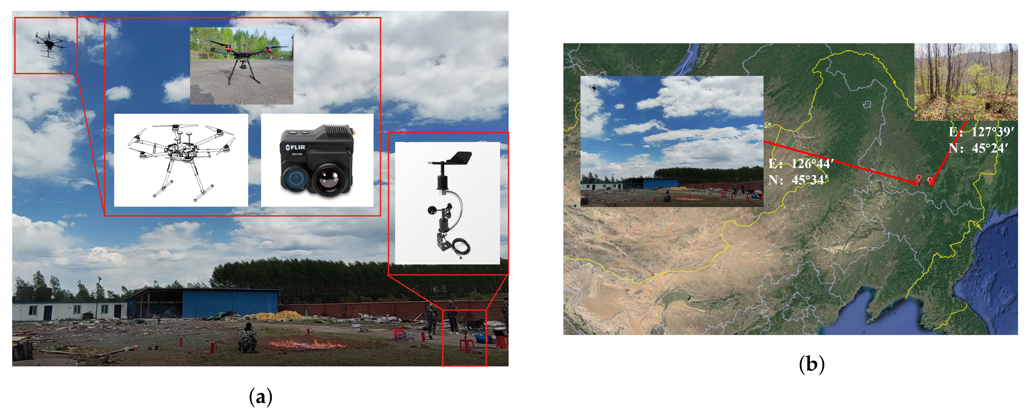
2.1. Burning Experiment Configuration

The surface fuel was selected from Maoershan, Harbin, Heilongjiang Province, China, 45 ° 24 N, 127 ° 39 E, as shown in Figure 1, in November (autumn). In order to fully verify the performance of the LSTM-based model in different scenarios, we collected the surface combustibles in coniferous forests mainly dominated by Pinus sylvestris var. mongolica [38,39] and broad-leaved forest dominated by poplars. The moisture of combustibles is measured with a drying method. Considering the applicability of the model, we choose the terrain slope and wind speed, which have great influence on the spread of forest fire, and they are easy to measure to set the experimental conditions to train the model. In different cases of forest fire spread, even if the wind speed and terrain slope are exactly the same, the estimated fire spread rate is also different due to the influence of other factors mentioned above which are not easy to measured, so the influence of these factors on fire spread can be regarded as the impact of the hidden layer parameters of the LSTM based model.
Configuration of the burning experiment is shown as Figure 1, and the experiment was carried out on 26 May 2021. A UAV is used to capture the whole process of fire spreading with the infrared camera, the camera parameters are shown in the Table 1. The fire spreading rate will be computed from the data of fire process, at the same time an anemometer is used to measure the wind speed. In order to simulate various environment variables in the actual forest fire spread as much as possible, such as the density and thickness of combustibles, air humidity, slope and so on, we set up the experimental group as shown in Table 2.
The type of anemometer is TGC-FSFX-C; it can capture both the direction and speed of the wind simultaneously. The anemometer is connected to the desktop with the linking of RS-232, and the data captured can be stored in the desktop in real-time. The absolute error of measured wind speed is less than 0.1 + 0.1 ϵ (m/s), where ϵ is the real wind speed, and 1 with respect to wind direction. The frequency for capturing data is 20 Hz. The anemometer is installed at 1.5 m above the ground.

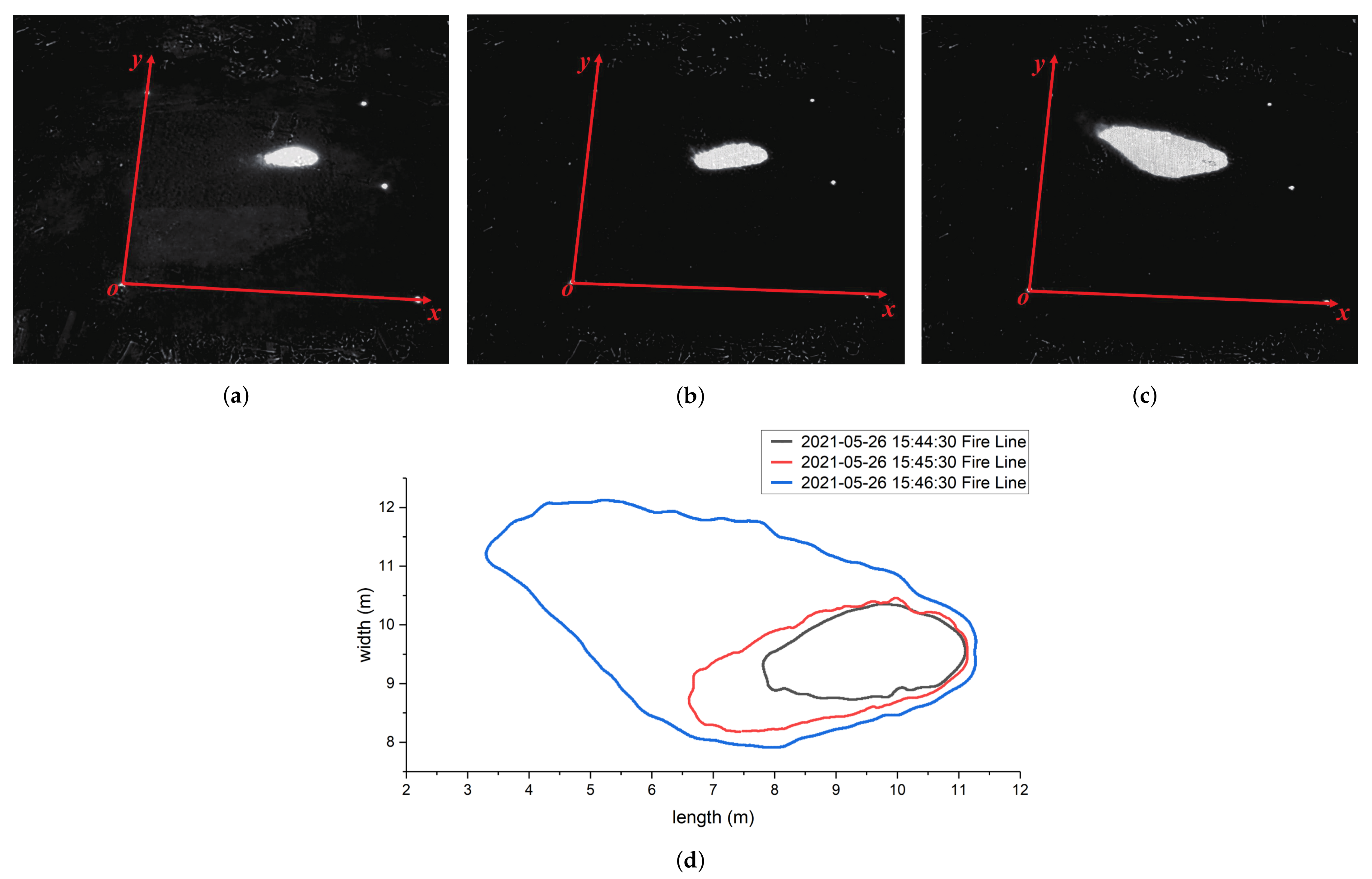
2.2. Computing Fire Spreading Rate from Sequences of the Infrared Images

It is easy to extract the fire front line from the infrared images with the threshold segmentation method; the fire spreading rate can be computed by differential method based on the time interval between two adjacent lines of fire. The UAV will tremble during capturing the fire spreading data, so the fire front line extracted from image must be transformed into the same coordinate system as that of the combustion bed. Four points are set in the bed for calibration, and these 4 points reveal very higher value in the infrared images. There are some noises in the raw infrared image, and median filter [40] method and other mutual algorithms [41,42,43,44] are used to filter the noises. After infrared images are preprocessed, the perspective transformation [45] is employed to compute the positions of fire in real word, Figure 2 shows 3 infrared images and their positions of the fire lines computed.
The infrared image can be preprocessed using the following median filter Equation (1), where w × w is the size of the sliding window on the infrared image. The median pixel value is selected from the window as the filtered pixel value.
g ( x , y ) = m e d { f ( x k , y l ) , ( k , l w ) ) }
The perspective transformation is usually used to compute the 3D coordinates of some pixels in the image, which is shown in Equation (2). x , y , z is the 3D coordinate, u , v is the pixel coordinate relevant to the 3D point and w is depth scaling factor which makes the pixel coordinate into the homogeneous format. a i , j in the right 3 × 3 matrix can be calibrated using the model data.
x y z = u v w a 11 a 12 a 13 a 21 a 22 a 23 a 31 a 32 a 33
For each experiment, both wind speed data and fire spread rate data are collected. As shown in Table 3, the statistical analysis results of 13 data sets are presented, which are mean value, standard error indicating the relative closeness of the value to the average, standard deviation indicating the overall fluctuation of the data and confidence interval. We can see that the value of fire spread rate is not only related to the wind speed, but also closely related to the experimental environmental conditions of this group. For example, in the first and second group of data, the average wind speed is close, but the fire spread rate is very different, which is caused by the different angle between the wind direction and the direction of fire spread in the two groups of experiments and other parameters. Because there are some outliers in the data set, it will affect the final convergence of the model. Therefore, we need to conduct standardized operations before we input data into the neural network, so that all inputs are similar in dimension distribution, thus allowing us to implement the same hyperparameter setting for each dimension in the network training process, which will achieve a good training effect. At the same time, we added the dropout structure to improve the fitting ability of the model for uncertain data.

3. LSTM-Based Model for Predicting Forest Fire Spread Rate

3.1. Normal LSTM-Based Model

The structure of LSTM contains total three gates controlling the cell state and hidden state. The Forget Gate determines how much information from the previous moment cell state can be passed to the current cell state. The Input Gate is used to control how much of the newly input information can be added to the current cell state. The Output Gate outputs the hidden state based on the updated cell state. In the normal LSTM-based model, fire spread rate and wind speed are trained and validated separately, according to the related sample data sets. The neuron unit structures are illustrated in Figure 3, for predicting fire spread rate and wind speed, respectively.
In Figure 3a, V F t represents the forest fire spread speed and C t records the information of forest fire spread speed with time t. In Figure 3b, the V W represents wind speed and C t records the information of wind speed change with time t. The ultimate goal of conducting forest fire spread research is to accurately predict the change of fire spreading rate so that fire prevention and extinguishing approaches can be arranged earlier. It can be seen from the figure that the wind speed and forest fire propagation rate are predicted independently, ignoring the mutual interaction in the actual wildfire. While learning the law of forest fire spreading, the main neuron merely optimizes the weight based on the forest fire spread rate self and cannot modify the rate according to the change of wind speed. When the wind speed changes, it will cause a change in the fire spread rate [46]. When the wind speed is introduced into the main neuron and then the weight parameters are corrected, the time lag is further increased, and, as a result, it is impossible to provide timely feedback on the predicted spread rate of forest fires. This is the main reason for developing improved LSTM-based models.
Taking the neuron unit for predicting fire spread rate for example, the control function of a single neural of LSTM is as the following Equation (3), and the neuron unit for predicting wind speed is same as that of the unit for predicting fire spread rate.
f t = σ ( W f V F t + R f h F t 1 + b f ) i t = σ ( W i V F t + R i h F t 1 + b i ) C ˜ t = tan h ( W c V F t + R c h F t 1 + b c ) C t = f t C t 1 + i t C ˜ t o t = σ ( W o V F t + R o h F t 1 + b o ) h F t = o t tan h ( C t )
In Equation (3), f t is the control function at the time t of the Forget Gate, and σ is the Sigmod [47] function, which generates a number between 0 and 1 to control the degree of forgetting state of the current cell. W f , R f and b f are weight matrices; V F t is the input of wind speed (it also applies to fire spread rate) at the current moment; and h F t 1 is the predicted output of the cell state at the previous moment. i t is the Input Gate control function, C ˜ t represents the update of the cell state, the function [48] generates a new candidate value represents the newly learned state after the forget gate f t is multiplied by the previous state C t 1 and the input gate i t is multiplied by new Cell State C ˜ t ; the updated cell state C t is computed. o t is the output Gate, and its output value is multiplied by the updated cell state to obtain the predicted value h F t at the current moment.

3.2. Improved Progressive LSTM-Based Models

Three progressive LSTM-based models for predicting the fire spreading rate will be introduced in this section, in which the interaction between wind and fire increases gradually. In order to make the main neural unit perceive the change of external wind speed while learning the law of forest fire spreading, we connect the output of accessory neural unit to the main neural unit to optimize the parameters. It is assumed that there is a certain degree of interaction between wind speed and fire spread rate, which is implied on the depth of the connection between the two neurons. The closer the connection between the two neurons, the more involved the two types of data are in the learning process of the neural network, and it also means that the interaction between wind speed and fire spread rate is stronger. According to the degree of connection between the two neural units, we have designed three kinds of progressive networks: (1) CSG-LSTM means that there is a certain interaction between wind speed and fire spread rate, (2) MDG-LSTM assumes that there is a strong interaction and (3) FNU-LSTM means that wind speed and fire spread rate always influence each other in the process of forest fire spread. The structures of the neural unit with respect to three kinds of LSTM-based model are detailed presented below.

3.2.1. CSG-LSTM with Combined Gate of the Same Type

According to structure of LSTM neural unit, the Forget Gate is used to control the cell state information forgotten from last time step. If the main neural unit is fully trained, then the rate of forest fire speed will also change in a period of time as a result of wind changing, which means there is a difference between the current state of the cell and previous time. The difference indicates that the output of the neural unit will show an upward trend at the current moment, increasing the degree of forgetting the cell state from the previous moment. At the same time, the Input Gate output of the neural unit should be decreased, and the degree of information input to the cell state at the current time step should be increased, so that the cell state of the main neural unit can be adapted to the development rule of the forest fire spread after the external wind speed changes as soon as possible. For the accessory unit, the change in wind speed will also cause the output of the Forget Gate to change; the performance of the entire model should depend on the main neural unit that predicts the rate of fire, so the Input Gate of the accessory unit should be related to the output of the main neural unit, and received performance feedback from the main neural unit. To sum up, the design of progressive neural unit (CSG-LSTM) is as Figure 4:
The forget gate control function is given by the accessory neural unit, so that the model can sense the change of external wind speed in real time, and accelerate the rate of learning the forest fire spreading speed after the main neural unit adapts the change of wind speed. The input gate control function is given by the main neural unit, which makes the model subject to the feedback of the main neural unit performance. The control function of CSG-LSTM neural unit is as follows:
Forget Gate:
f t = σ ( W f V W t + R f h W t 1 + b f )
Input Gate:
i t = σ ( W i V F t + R i h F t 1 + b i ) C ˜ t = tan h ( W c V W t + R c h W t 1 + b c ) C ˜ t = tan h ( W c V F t + R c h F t 1 + b c )
Update Cell State:
C t = f t C t 1 + i t C ˜ t C t = f t C t 1 + i t C ˜ t
Output Gate:
o t = σ ( W o V W t + R o h W t 1 + b o ) h W t = o t tan h ( C t ) o t = σ ( W o V F t + R o h F t 1 + b o ) h F t = o t tan h ( C t )
Equations mentioned before illustrate how to get the predicted fire spread rate and wind speed based on current input and cell state information recorded in last time step. C t stores the information that the wind speed changes with time, o t is the control function of the accessory neural unit’s Output Gate, h W t is the predicted output of the accessory neural unit w.r.t. wind, C t stores the information of the change of the forest fire speed with time, o t is the output gate control function of the main neural unit and h F t is the predicted output of the main neural unit about fire spread rate.

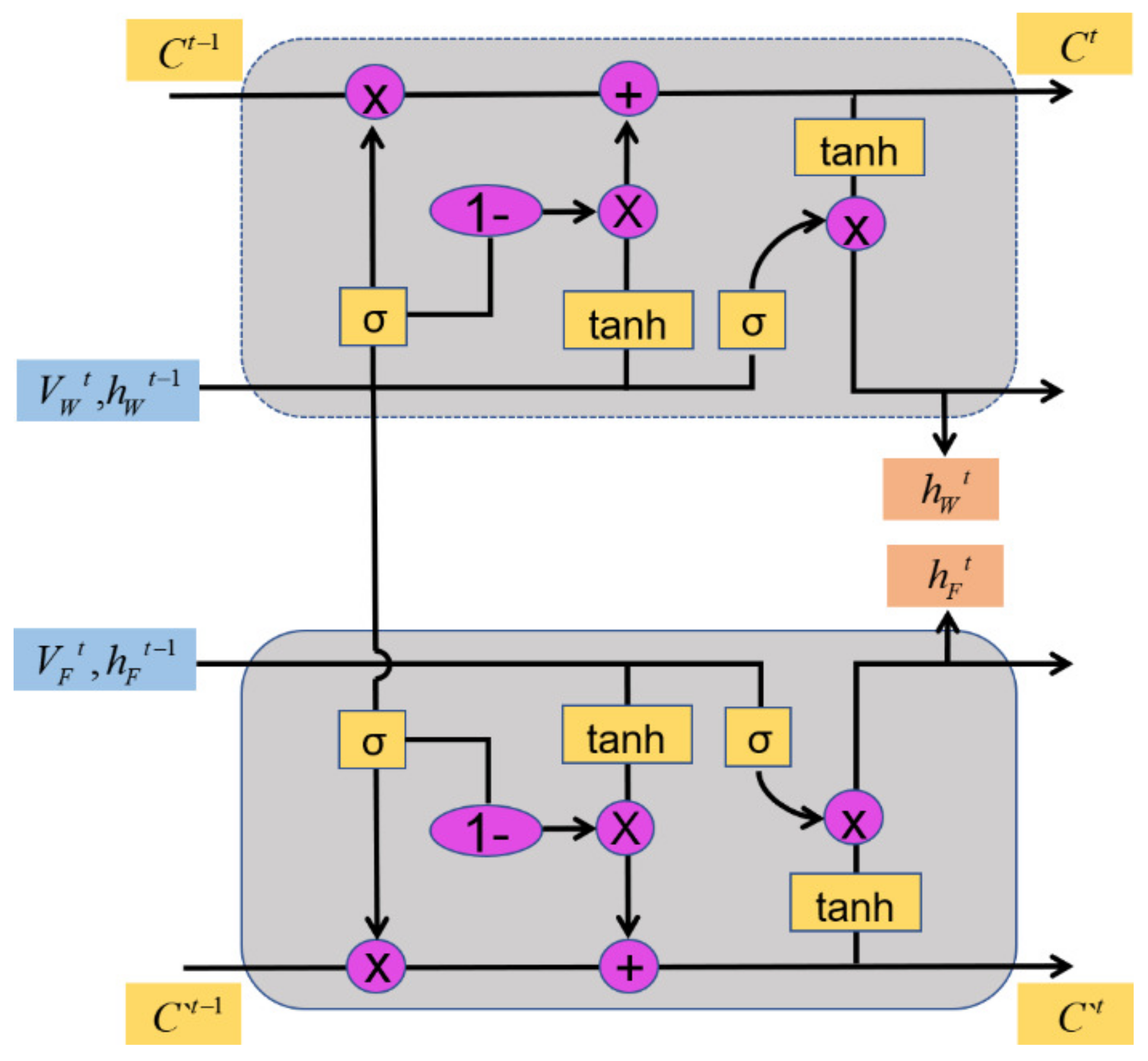
3.2.2. MDG-LSTM with Combined Gate of the Different Type

Kyunghyun Cho proposed the Gate Recurrent Unit model (GRU) [49], which revised three gate functions of LSTM. This model can not only effectively solve the problem of the gradient disappearance, but also simplifies the calculation process and improves the operation speed. Among them, the Update Gate function is used to determine the information that should be updated, which is equivalent to the combination of Input Gate and Forget Gate in the LSTM network; the Reset Gate function is used to control the discarded information. Structure of the GRU neural unit is shown as Figure 5:
It can be seen from the Figure 5 that the “1−” operation is carried out when calculating the hidden state. We suggest that the newly added information has the opposite trend of weight calculated when updating the unit state and output. Therefore, in order to reduce the number of parameters and improve the speed of operation, “1−” is introduced in the hidden state. In the CSG-LSTM designed in Section 3.2, although the main neural is able to perception and respond to changes in external wind speed while learning, the hidden parameters increase exponentially due to the link between the two neural, and the amount of computation is too large. In order to reduce the amount of computation without affecting the perception of the main neural to the change of wind speed, using the design idea of GRU for reference, the “1−” is can be introduced into the control weight of the Input Gate, and the design MDG-LSTM is shown in Figure 6.
On the basis of the CSG-LSTM, the model connects the Forget Gate with the Input Gate through the “1−” operation; on the one hand, it reduces the number of parameters that need to be optimized and speeds up the iterative process, and on the other hand, the wind speed data can better participate in the optimization process of the whole model. The detailed formula of MDG-LSTM is as follows:
Forget Gate:
f t = σ ( W f V W t + R f h W t 1 + b f )
Update Cell State:
C ˜ t = tan h ( W c V W t + R c h W t 1 + b c ) C ˜ t = tan h ( W c V F t + R c h F t 1 + b c ) C t = f t C t 1 + ( 1 f t ) C ˜ t C t = f t C t 1 + ( 1 f t ) C ˜ t
Output Gate:
o t = σ ( W o V W t + R o h W t 1 + b o ) h W t = o t tan h ( C t ) o t = σ ( W o V F t + R o h F t 1 + b o ) h F t = o t tan h ( C t )
C t still stores dynamic change information of the wind speed, and C t stores dynamic change information of the forest fire spread rate. In general case, Input Gate is hidden , and “1−” operation with Forget Gate is applied to update current state. The Forget Gate weights of the main neuron and the accessory neuron are controlled by the accessory neuron Forget Gate. Speed of weight updating is still controlled by predicted output of the main neuron.

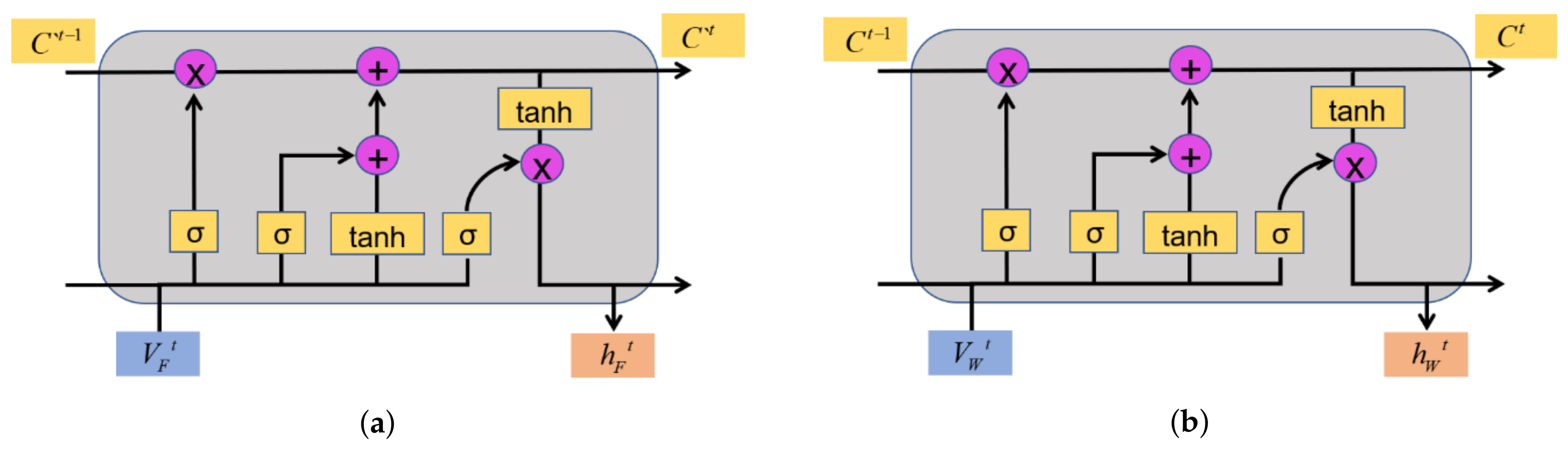
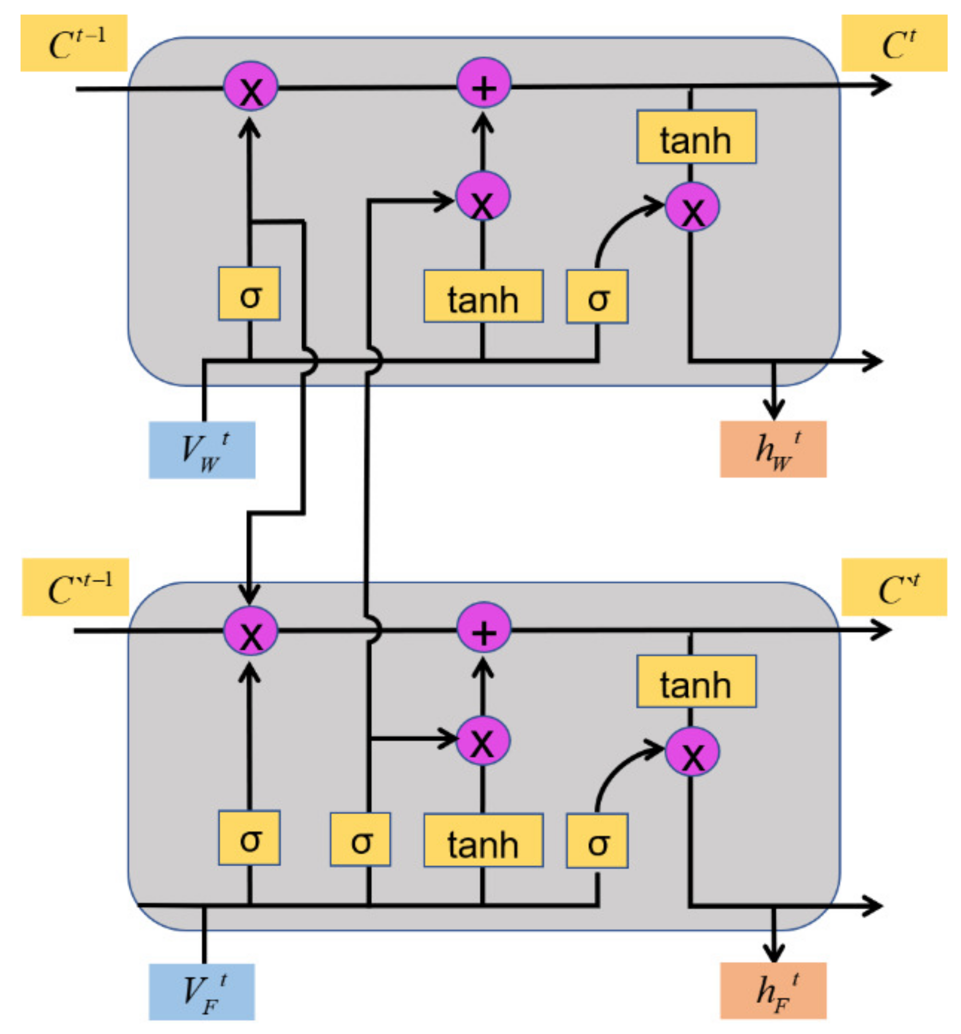
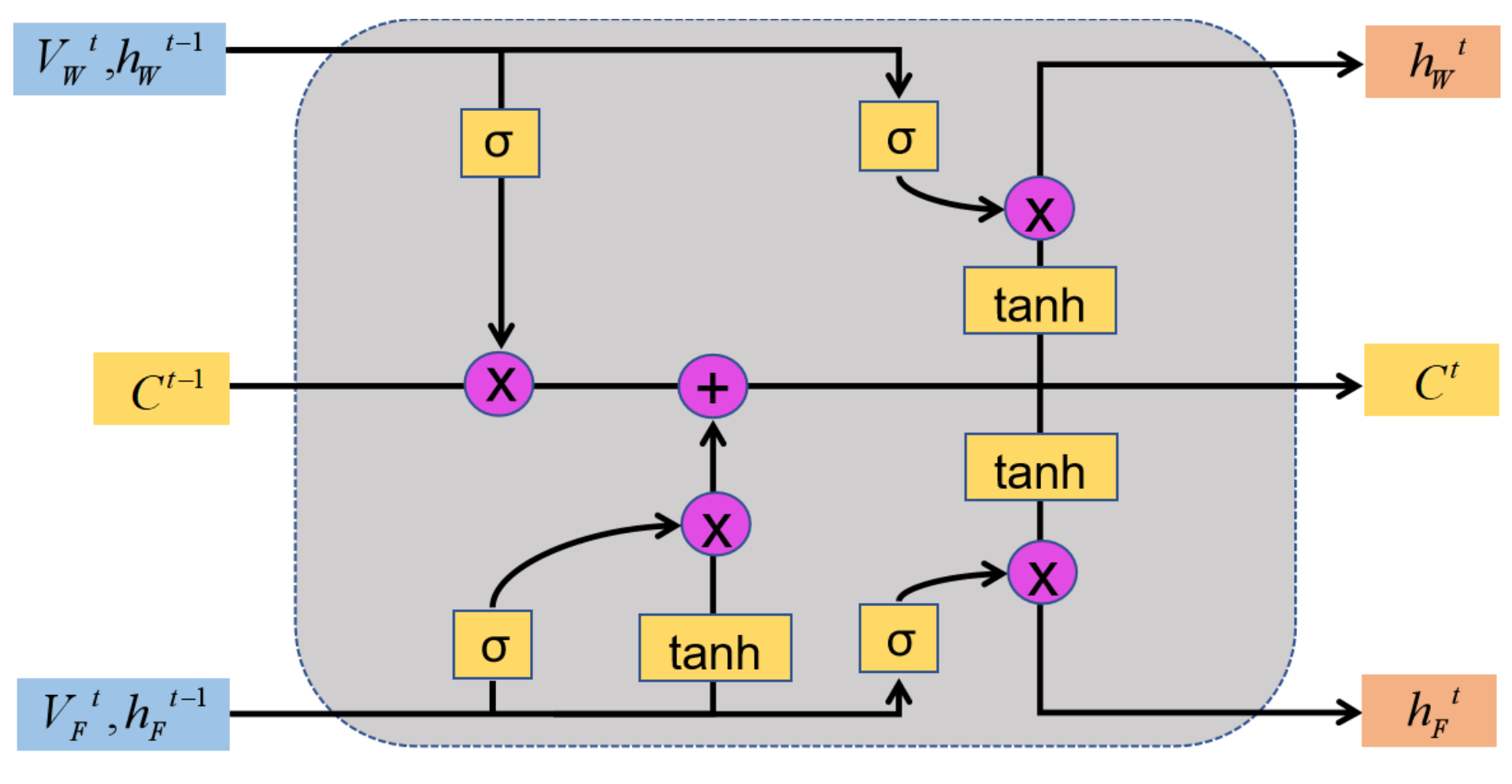
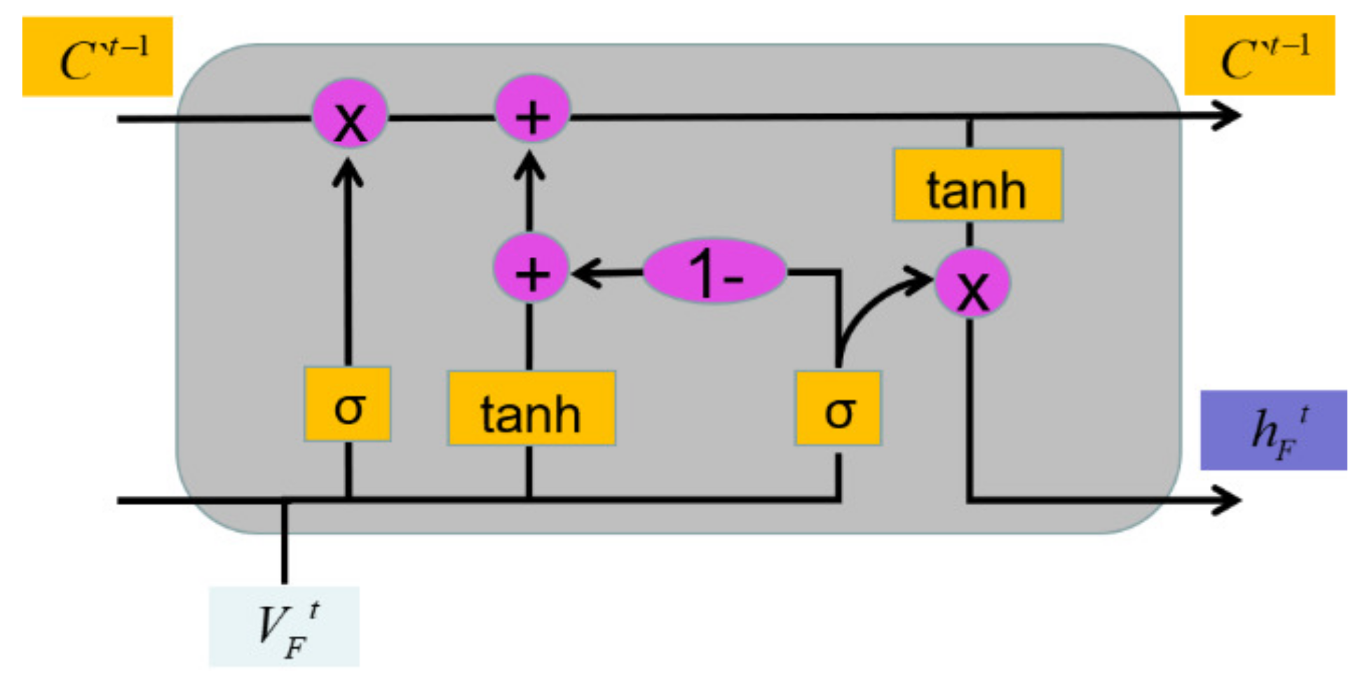
3.2.3. FNU-LSTM with Fusion of Two Neural Units

In the structure of MDG-LSTM, both main neural unit and accessory neural unit share the same Forget Gate based on accessory neural unit. Under this structure it is considered that there is a strong interaction between the wind speed and the forest fire spread rate, in other words, the change of the wind speed will cause the change of the forest fire spread rate, and at the same time, the local wind speed of the fire site will be affected by the feedback of the flame. By further enhancing interaction between fire spread rate and wind speed, we can use the same cell state to record both of their changes. The LSTM neural unit (FNU-LSTM) that combines the main neural and the accessory neural is designed as Figure 7.
As shown in Figure 7, we further compress two independent neurons into a progressive neuron, in which the wind speed controls the Forget Gate of the neural, while the fire spread rate controls the Input Gate of the neural unit. The two inputs show a progressive relationship in logical operation. The detailed formula of FNU-LSTM is as follows:
Forget Gate:
f t = σ ( W f V W t + R f h W t 1 + b f )
Input Gate:
i t = σ ( W i V F t + R i h F t 1 + b i )
Update Cell State:
C t = f t C t 1 + i t C ˜ t
Output Gate:
o t = σ ( W o V W t + R o h W t 1 + b o ) h W t = o t tan h ( C t ) o t = σ ( W o V F t + R o h F t 1 + b o ) h F t = o t tan h ( C t )
The control function f t of the Forget Gate is generated by the wind speed V W , which is used to detect the change of the external wind speed and control the retention degree of the previous cell state C t 1 . The control function i t of the Input Gate is related to the speed of forest fire spread V F , and controls the degree of information inputting into the cell state at the current moment according to predictive output of the last time step. Two Output Gates are set to control wind speed and forest fire spreading rate predicted respectively. Under this model structure, it is assumed that there is a strong interaction between wind speed and forest fire spread rate.
Three kinds of LSTM-based model share the same type of input and output data. There are 4 inputs: the fire spread rate and wind speed predicted from the last round, the fire spread rate and wind speed measured this time. There are 2 outputs: the fire spread rate and wind speed predicted this time. In practice, two neuron units are connected continuously, so there is no measured spread rate and wind speed passing to the input of the latter neuron unit. Of course, you can make more neuron units connected to predicted fire spread rate a long time later.
Take the third model FNU-LSTM as the example. In the revised manuscript, Equation (11), Equation (12), Equation (13) and Equation (14) present the computing process of the model FNU-LSTM, which coordinate with the Figure 7. Equation (11) describes how to compute the forget gate, which is associated with the wind speed predicted in last round and measured this time. Equation (12) describes how to compute the input gate, which is associated with the fire spread rate predicted in last round and measured this time. Equation (13) describes how to update the cell state based on the forget gate and input gate. Unlike the forget gate and input gate, in Equation (14), the output gates for controlling fire and wind are separated each other. The output gate of fire speed is computed based on the fire spread rate predicted in last round and measured this time, and that of wind speed is based on the wind speed predicted in last round and measured this time. All the symbols like W, R and b in such equations are the weights needing to be trained on the data set
The LSTM-based model proposed in the manuscript can be extended to be used in the real application. Once the weight parameters were trained in advance, the time series of the fire spread rate can be predicted based on the input of historical time series of the fire spread rate. In the general case, a UAV can be used to measure the fire spread rate for a period, and then the model can predict the fire spread rate in the future time, the experiment section has validated the scalability to the wildland fire prediction. In addition, the extreme fire behaviour with sudden change of the fire spread rate often brings great thread to the firemen, and this model can predict this extreme case.

4. Result and Analysis

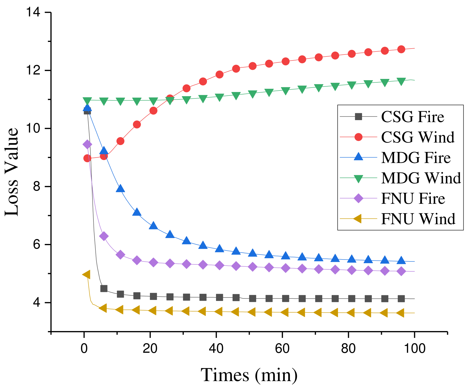
4.1. Analysis of Loss Value for Training the LSTM Based Models

The loss function is an important parameter in deep learning. Parameter learning of the network is driven by a back propagation algorithm, which need data sample pairs of predicted and real values. In the training stage, the Cross-Entropy Loss [50,51] is used to describe the error changes in the learning process of three different progressive LSTM neural networks. The Cross-Entropy Loss is presented as follows:
L s o f t m a x L o s s = 1 N l o g ( e y i Σ j = 1 C e j )
LSTM networks are trained based on one data set which includes over 1000 pairs of (input, output), there are 4 kinds of data int the input including the fire spread rand and wind speed predicted from last time step, and the values measured at this time step. The output includes the fire spread rand and wind speed predicted at this time step. All the loss values are recorded in the whole training process. Changing curves of loss value w.r.t. 3 kinds of LSTM-based models are shown in Figure 8.
In the training progress, the CSG-LSTM takes about 100 iterations and 13 min to reach the limit convergence value of fire spread rate. As can be seen from Figure 8, when iterating for about 10 times, the convergence value of fire spread speed can reach 4.5, while the convergence value of wind speed increases to more than 12.6. This is because in the model unit structure of CSG-LSTM, the forget gate is used to put the change of wind into the main cell unit for predicting the fire spreading rate. It is unsatisfactory for the accessory cell unit to learn to predict the wind speed. Therefore, it is necessary to optimize the structure of CSG-LSTM, making full use of wind fire interaction mechanism, which is the reason for designing MDG-LSTM and FNU-LSTM.
In the training progress of MDG-LSTM model, it takes about 100 iterations and takes 160 min to reach the limit convergence value of fire spread speed. Compared to that of CSG-LSTM, the convergence rate of the fire spreading speed becomes slower. At the same time, the loss value of the wind speed has not increased much, and it is maintained at around 11.4. In the neural unit structure of MDG-LSTM, the connection between the accessory cell unit and the main cell unit is further deepened, and the control functions of the Forget Gate and Input Gate of the accessory cell unit and the main cell unit are controlled by the Forget Gate of the accessory cell unit. Under this cell structure, the accessory neural unit can not only play an auxiliary role in the learning process of the main cell unit, but also accept the learning feedback of the main cell unit very well, so the accessory neural unit has a certain direction for the learning convergence of wind speed and is no longer rising blindly. Compared with the CSG-LSTM model, under the assumption that there is a strong interaction between the wind speed and the fire spread rate, the model further deepens the relationship between the two neural units, and more data of the wind speed and fire spread rate participate in the training of the whole model. It can also be seen from the functional relationship that the algorithm of this model is more complex than the CSG-LSTM model, so this model needs more time to get a better convergence.
In the training progress of FNU-LSTM model, it takes about 10 iterations and 20 min to reach the convergence value of fire spread speed. In FNU-LSTM, the learning of wind speed and fire spread speed is carried out by the same cell unit, which undoubtedly deepens the interaction between wind speed and fire spread rate. Under this structure, the iteration of the whole model can be promoted only if there is a strong relationship between the two kinds of data. Input wind speed data to the Forget Gate which enables FNU-LSTM to sense the changes of external environment conditions and assist the learning of fire spread speed. The Input Gate with input fire spread speed data makes it possible to adjust the state of cell units according to the change of loss value in the training process, and the structure of this single-cell unit can learn the interaction between wind speed and fire spread speed. This also proves that our inference about wind speed and fire spread rate is correct, and it is precisely because of the strong interaction between them that the FNU-LSTM model can achieve better results compared with the above two models.
Based on the interaction between wind speed and forest fire spread rate in the process of forest fire spread, by observing the change of loss value of three progressive LSTM models describing different degrees of the interaction, it can be seen that FNU-LSTM model has better learning ability, and it is also proved that there is a strong interaction between wind speed and fire spread rate.

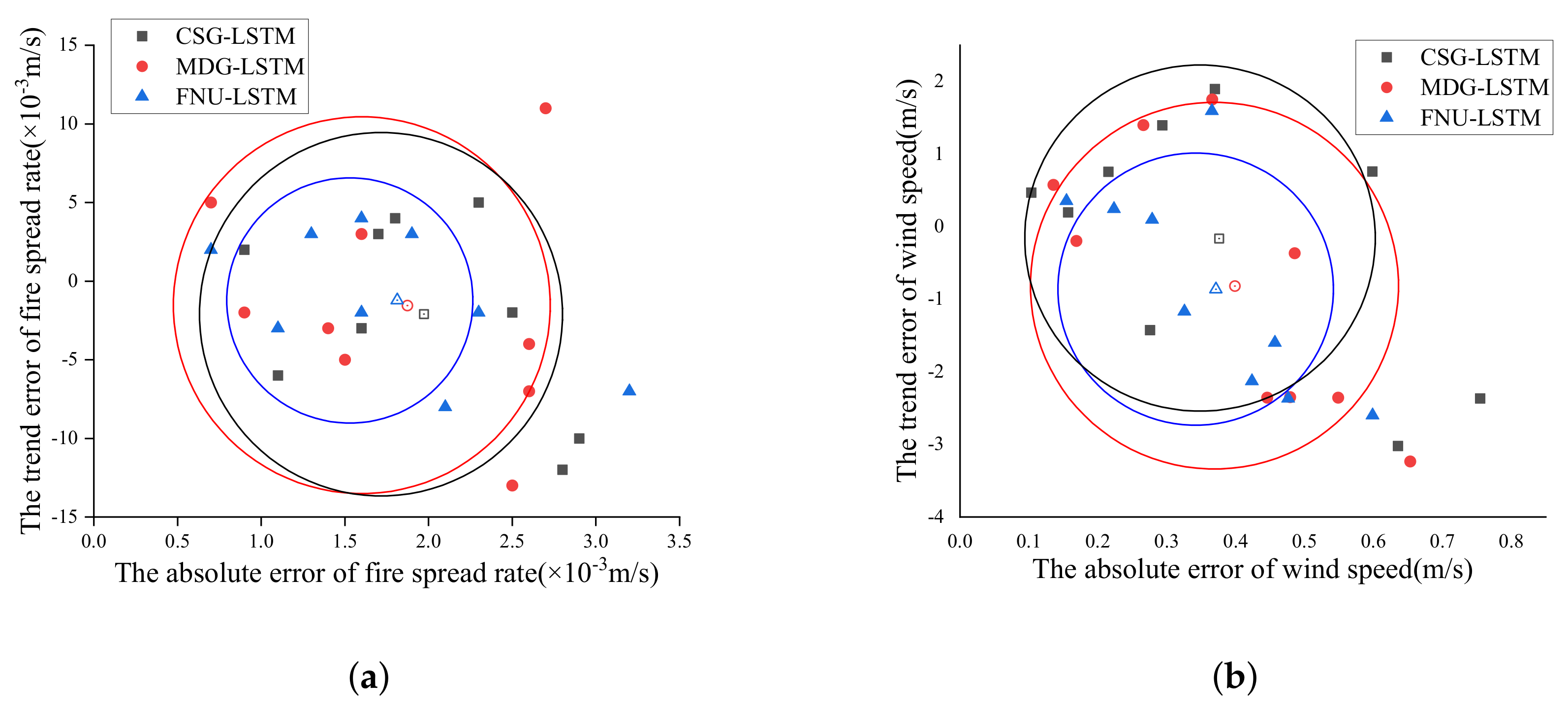
4.2. Error Analysis of LSTM Based Models

In this section, we will use the data set obtained from the combustion experiment to train the three LSTM neural networks with progressive structure proposed above, and measure which model is more advantages from the two aspects of prediction accuracy and model generalization ability. Each data set includes about 10 min of time series data in seconds. To save training time, 5 s is used as an LSTM unit time, and the learning rate is set as 0.005.

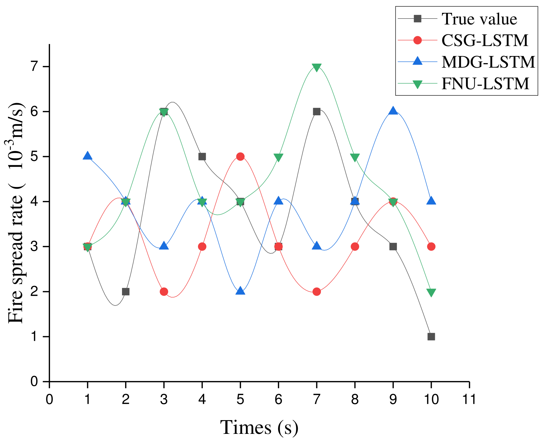
4.2.1. Predicting Error

The training is stopped when the loss value reaches the limit convergence point. In this subsection, five data set that are different from the training data set are used to predict both fire spread rate and wind speed, loss value, absolute error and trend error are computed simultaneously. Figure 9 shows the true value and predicted value of three improved LSTM models.
The truth value in Figure 9 comes from the experimental data. When the loss value reaches the limit convergence point, we will use the test set as the input of the model to predict fire spread rate. The absolute error is used to measure the relative distance between the predicted value and the actual value. Finally, the average value is computed based on thirty series of fire spreading process data. The trend error is directly measured by the difference between the true value and the predicted, which reflects ability of the predicted value to fit the trend change of the true value, and finally the total value is taken to reflect the ability of the model to describe the data trend in the thirty time series. Through training projections from three neural networks models with 9 datasets we can eventually obtain 27 groups of data as shown in Table 4, Table 5 and Table 6, respectively.
As can be seen from the Table 4, Table 5 and Table 6, although the fire loss value of FNU-LSTM are the biggest which compared with the other two models, this is because the difference in resolution accuracy between wind speed data and fire spread data. There is no measuring unit for loss value, which is obvious from the Equation (15). At the same time, the loss value in the training process cannot be regarded as the main index to measure the performance of a model. In the following part, the generalization ability of the model will be discussed in detail.

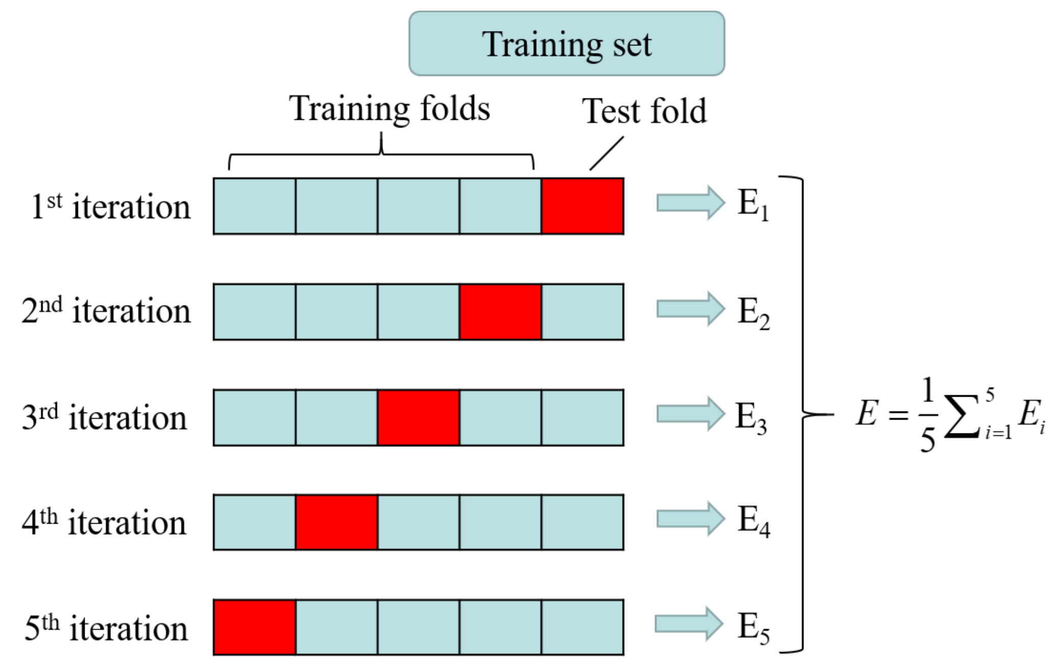
4.2.2. Generalization Ability of the Model

In order to further validate generalization ability of the model for data sets, the concept of “gravity center” is introduced. We assume that each data pair is a particle, the absolute error is the abscissa value x of the particle, the trend error is the ordinate value y of the point and the loss value is the weight m of the particle. In this way, particle error points of each model can be scattered in the plane, and we can obtain the gravity center of the scatter graph.
G x = 1 9 m i * x i M G y = 1 9 m i * y i M
In Equation (16), M is the total number of particles. Let ( G x C S G _ F , G y C S G _ F ) denotes the error gravity center of fire spread rate predicted by CSG-LSTM model, and ( G x C S G _ W , G y C S G _ W ) denotes the error gravity center of wind speed predicted by CSG-LSTM model. The error gravity center about other models is represented using the same format.
All the gravity centers are listed below:
( G x C S G _ F , G y C S G _ F ) = ( 1.972 , 2.102 ) ; ( G x C S G _ W , G y C S G _ W ) = ( 0.376 , 0.162 ) ;
( G x M D G _ F , G y M D G _ F ) = ( 1.873 , 1.546 ) ; ( G x M D G _ W , G y M D G _ W ) = ( 0.399 , 0.816 ) ;
( G x F N U _ F , G y F N U _ F ) = ( 1.813 , 1.217 ) ; ( G x F N U _ W , G y F N U _ W ) = ( 0.371 , 0.863 ) ;
The gravity centers and particle error points are scattered in Figure 10. In each scatter plot in Figure 10, the solid symbols represent error particle points and the hollow symbols represent gravity centers.
Now, we are going to list error range for each model; let E A b s C S G _ F denote the absolute error of CSG-LSTM model and E T r e C S G _ F denote the trend error of prediction. Other errors are represented using the same style.
All the error range distributions are listed below.
E A b s C S G _ F ( 0.9 , 2.9 ) , E T r e C S G _ F ( 12 , 5 ) ;
E A b s C S G _ W ( 0.104 , 0.755 ) , E T r e C S G _ W ( 3.023 , 1.897 ) ;
E A b s M D G _ F ( 0.7 , 2.8 ) , E T r e M D G _ F ( 13 , 11 ) ;
E A b s M D G _ W ( 0.136 , 0.653 ) , E T r e M D G _ W ( 3.235 , 1.655 ) ;
E A b s F N U _ F ( 0.7 , 2.6 ) , E T r e F N U _ F ( 8 , 4 ) ;
E A b s F N U _ W ( 0.205 , 0.599 ) , E T r e F N U _ W ( 2.596 , 1.833 ) ;
In terms of error distribution range distance, we find that the error of FNU-LSTM model for predicting forest fire spread rate is always smaller than that of the other two models, so it has higher accuracy for ability of predicting fire spread rate.
In the error distribution diagram, we take the gravity center as the center of the circle, covering 6 points with the smallest distance from the gravity (the farthest point falls on the boundary of the circle), as shown in Figure 10. The circle centered at the gravity center represents the density of error distribution, the smaller the circle, the more reliable the model.
We measure the distribution density of the error from two aspects, the first one is the radius of the error circle, and the second one is the average error distance.
The radii of the error circles are compared among these 3 kinds of improve LSTM based models as below.
R F N U _ F < R C S G _ F < R M D G _ F ;
R F N U _ W < R C S G _ W < R M D G _ W ;
The radius of the error circle by FNU-LSTM is smaller than that of the other two models. The average error distance of each point in the circle relative to the center of gravity are listed below.
d F N U _ F < d M D G _ F < d C S G _ F ;
d F N U _ W < d C S G _ W < d M D G _ W ;
In summary, the error distribution of FNU-LSTM is more concentrated, and the error distance is relatively short, which means that the model has more stable data learning ability and higher accuracy when applied to predict forest fire spread rate under many different environmental conditions, so FNU-LSTM has stronger applicability and generalization ability than the other two models.

4.3. Optimizing Hyperparameters of Improved LSTM Based Model

Hyperparameter optimization is a key step for improving the prediction model; here, the number of hidden neural units and the learning rate are considered to be optimized. For the weight initialization before training model, we employ two assignment methods: standard normal distribution and truncated normal distribution.
Cross-Validation [52] is used to evaluate the trained models. We divide the original data into five groups, as shown in the Figure 11; each subset of data is validated once; and the remaining four subsets of data are used as training sets.
Cross-Validation error is computed by averaging every evaluated results. Considering the randomness of the initial weight assignment, each model is trained three times with different hyperparameters, the optimal one are selected as the final hyperparameters. Table 7 shows our training results after Cross-Validation, when the hidden neural unit is set to 10 and the learning rate is set to 0.0006, the model initialized by truncated normal distribution can achieve better performance.

4.4. Comparing Experiments

In order to fully validate prediction ability of the model FNU-LSTM, comparison experiments are carried out between FNU-LSTM and other LSTM-based models based on both burning data and wildfire data.

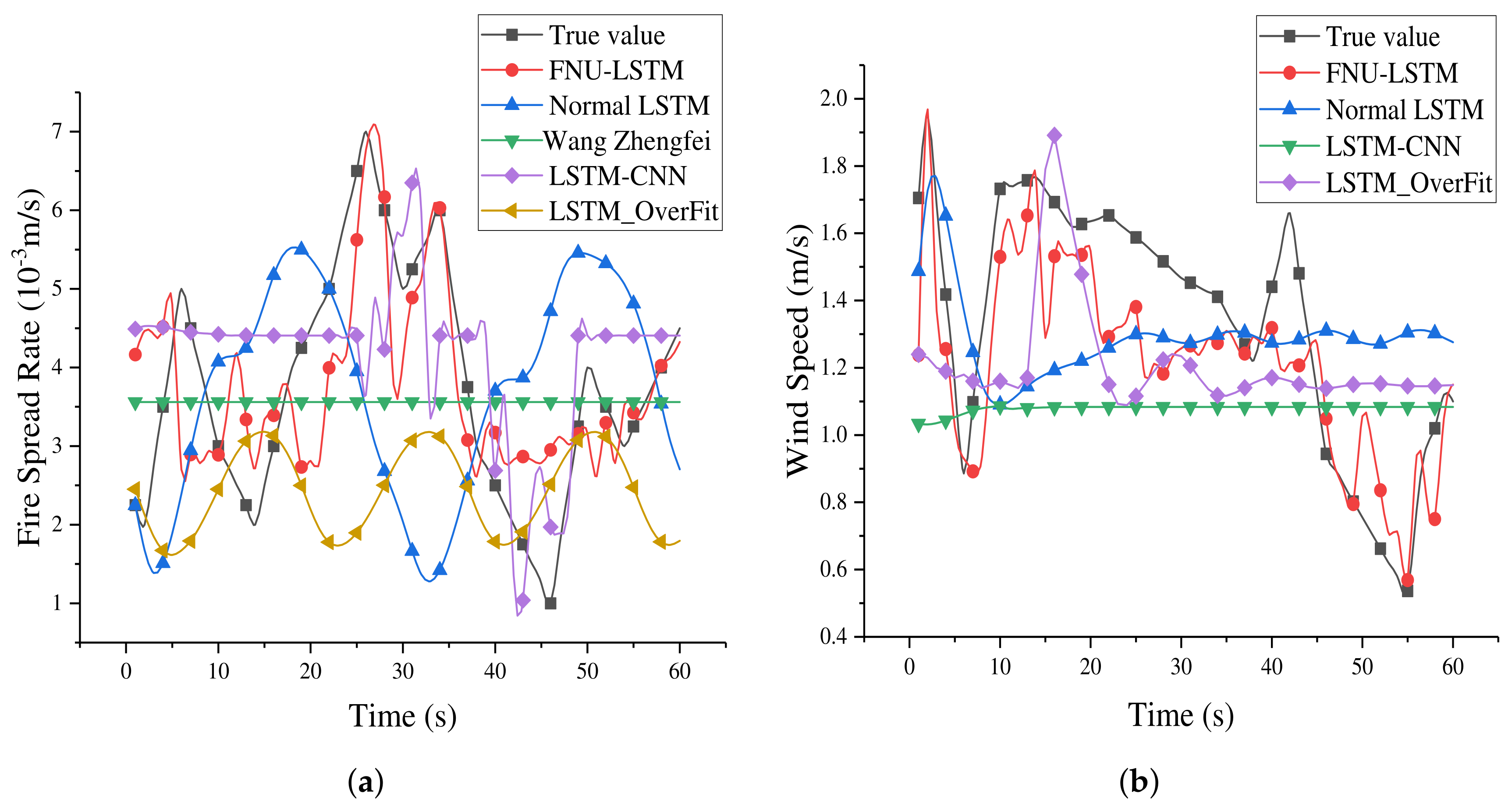
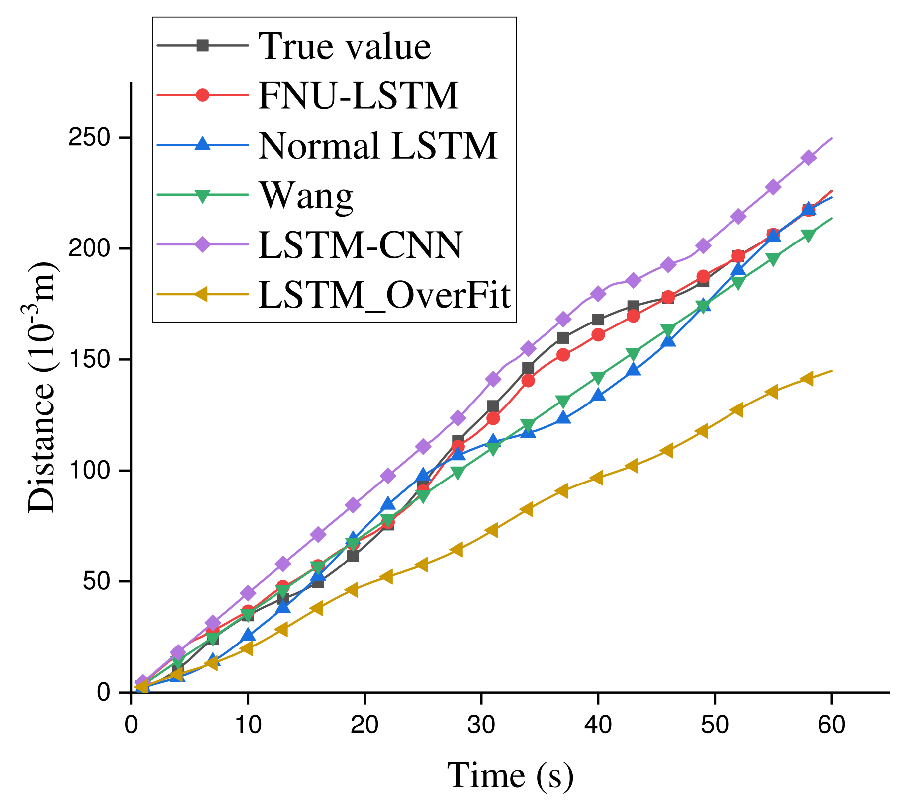
4.4.1. Comparison Based on the Data from Burning Fire Experiment

LSTM-CNN [53,54], a model used to detect traffic related microblogs from Sina Weibo, adds a convolutional layer and a pooling layer after LSTM output. In the model, CNN can further extract deep features and add its input to the fully connected neural network. LSTM-OverFit [55], a model combining overfitting functions and full concatenation functions, is used to predict the spatial and temporal effects of related variables in earthquakes. By referencing advice mentioned in the original papers, here, hyperparameters for all the models are shown in Table 8.
Predicted results lasting for 60 s are acquired using the trained models, which are shown in Figure 12. In addition to the LSTM-based models, a classical mathematical model Wang Zhengfei all takes part in the comparison experiment, and related parameters include Temperature (9.5 ° C), Global wind speed (2.5 m/s), Air humidity (39.5%) and Slope inclination (15 °). At the same time, we calculate the RMSE value of each model relative to the true value, which can reflect the accuracy of model prediction, shown in Table 9.
As can be seen from Figure 12a, compared with the traditional mathematical Wang Zhengfei model, neural network has great advantages for studying the changes of fire spreading tend. The trend change predicted by FNU-LSTM is similar to the true value obtained from the burning experiment, and the error distance about the true value is also smaller than that of other models. Figure 12b also shows an advantage when predicting wind speed, compared to other LSTM-based model. Figure 13 shows the performance of the neural network model for distance simulation. Final prediction results of LSTM and LSTM-OverFit are very similar, but because the fully connected layer added by LSTM-OverFit can deepen the learned features, the predicted output of LSTM-OverFit is closer to the true value. However, compared with true value, these two models can only simulate a general trend and cannot accurately reflect the changes of fire spread rate or wind speed due to these models cannot perceive the change of the external wind speed. For the LSTM-CNN model, its prediction results are quite different from the true value; that is because the added convolutional layer extracts feature too much, and the original model does not prevent overfitting operations, resulting in the poor performance of the model in the data set. There are two mainly factors contributing to this phenomenon. In this paper, the flame spread speed date extracted into the neural network is realized by threshold segmentation in the data preprocessing. We do not use a convolutional neural network to extract the features of the image, so this data processing method does not give full play to the advantages of LSTM-CNN. Furthermore, this relatively poor performance can be seen as the result of a difference focus on the characteristics of the data. In the spread of forest fire, we are more concerned about the speed of fire spread, that is, the flame moves form position A at the current moment to position B at the next moment. We are focused on how the flame behaves during this period of time. Therefore, even if we use convolution network for data preprocessing, the data features extracted by CNN may not be the features we need in this paper. To sum up, the well-known LSTM-CNN model cannot achieve an expected performance in the field discussed in this paper. However, we still believe LSTM-CNN has a very strong ability to process image time series and has great advantages in image processing and classification.

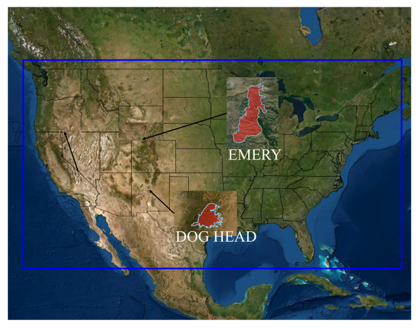
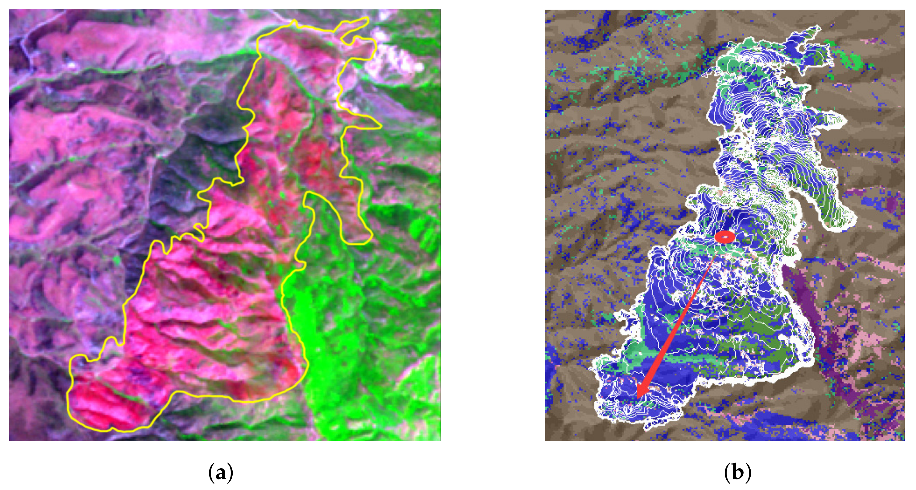
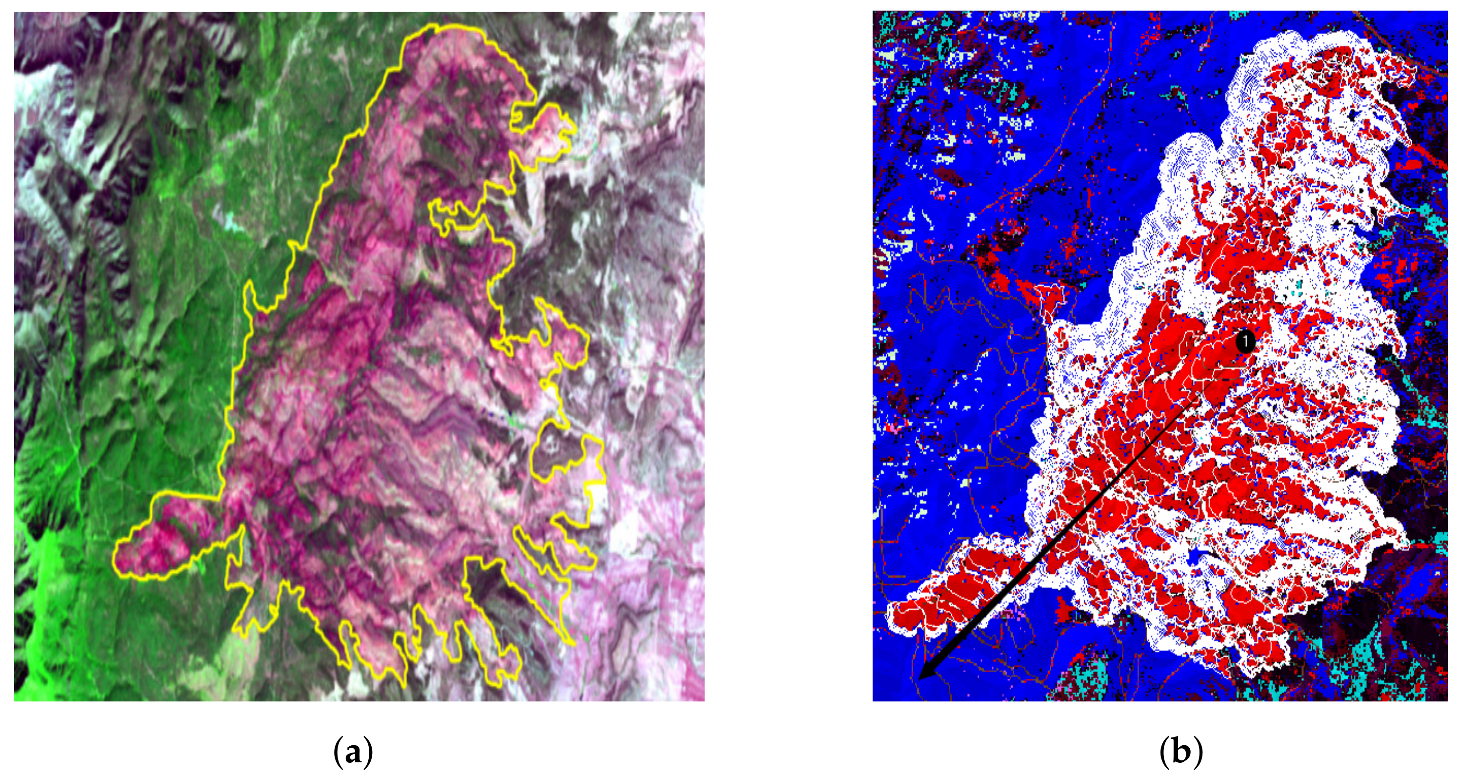
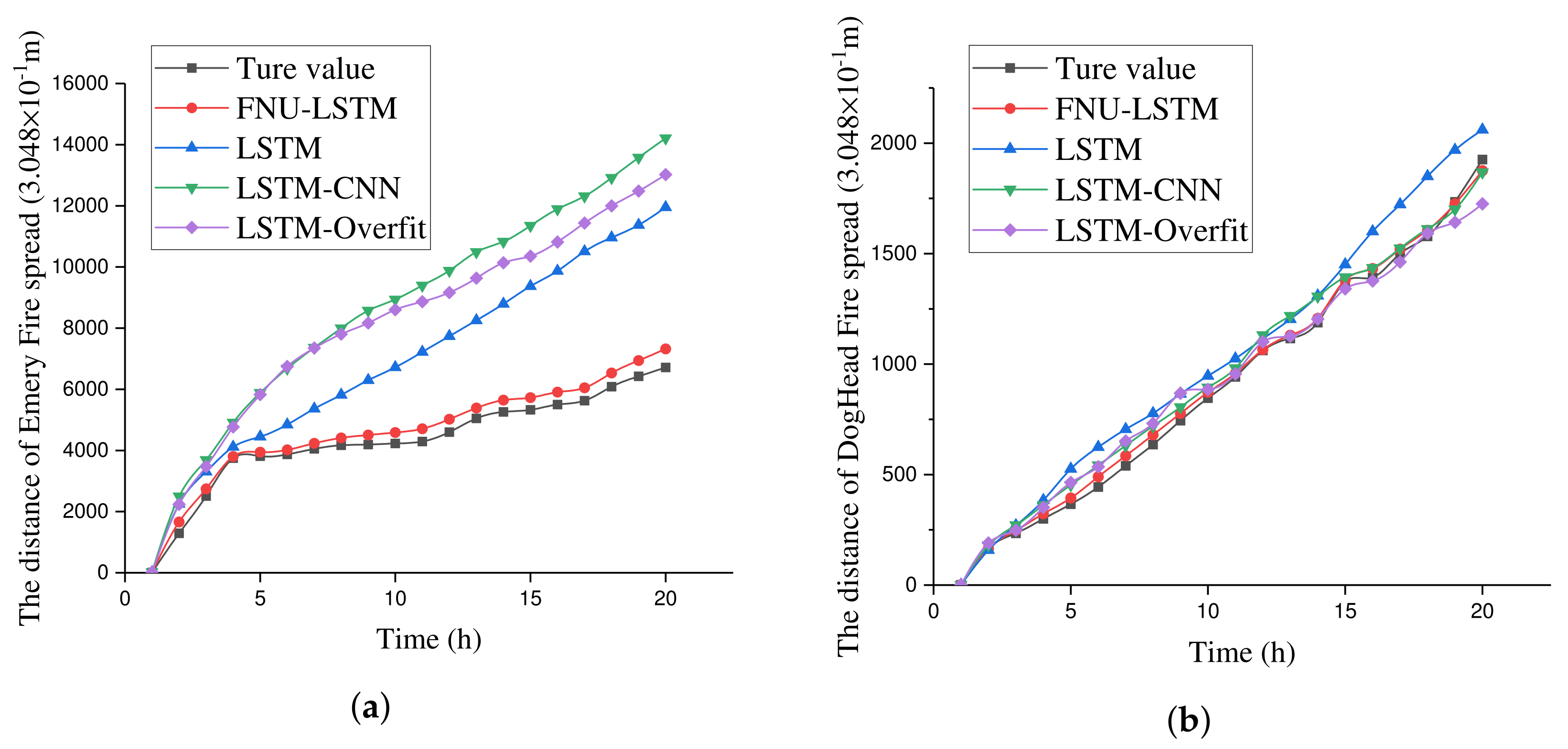
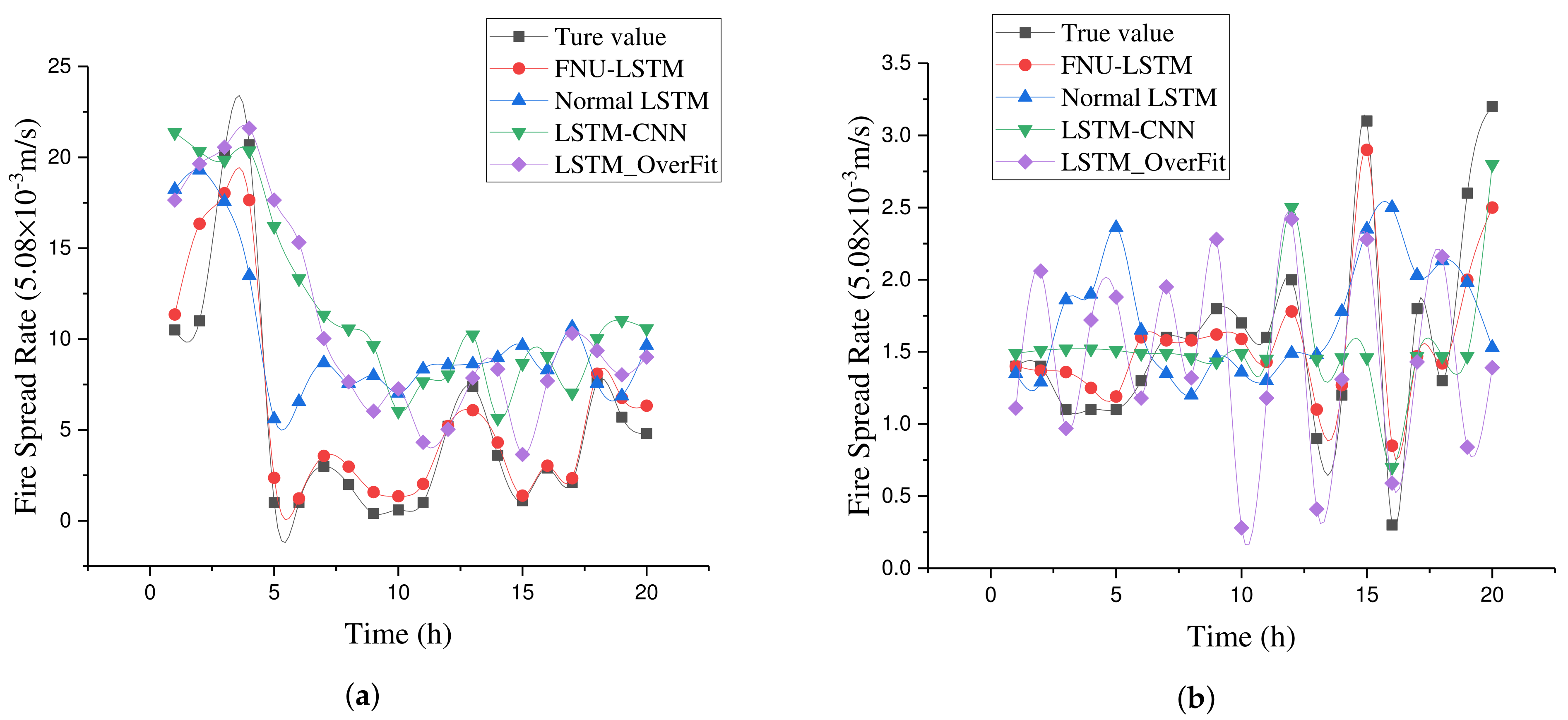
4.4.2. Comparison Based on the Data from Wildland Fire

Through the above outdoor burning experiments, we have obtained an FNU-LSTM model with high enough accuracy to predict fire spread rate. In order to verify applicability of the model FNU-LSTM, we find two wildland fires which are different in area, topography, climate and fire occurrence from Monitoring Trends in Burn Severity (MTBS) website, the two wildland fires as shown in Figure 14. We use Farsite to import the relevant data to simulate the two fires, in which the Rothermel model is used to calculate the fire spread rate, and the Huygens model is used to simulate the spread of the fire boundary, as shown in Figure 15 and Figure 16. The results are very similar to the final combustion boundary of the original fire, so we suggest that the linear velocity of fire obtained in the simulation can be used as the real speed of fire. Topography, vegetation, fuel and meteorological data related to the wildland fires were downloaded from LANDFIRE, including all the wind speed data needed for training, at RAWS USA Climate Archive. The humidity data of different combustibles were obtained from the National Fuel Moisture Database. The start and end time of the fire and the location of the fire point were obtained from FIRE & WEATHER DATA to ensure that the setting time and location of the fire simulation are consistent with the actual situation.
For the color in Figure 15 and Figure 16, Figure 15a and Figure 16a shows the remote sensing image of historical fire sites (Landsat 5), the pixel value (i.e., color) of the image is scaled according to the vegetation type, and the region after the fire is different from that before fire through scaling operation, the recognition degree of the fire region is very high, as covered by the yellow envelope line. The both Figure 15b and Figure 16b are simulation environment of Farsite which is a famous software for simulating forest fire spreading, it is used to generate the fire spreading data for training and validating the LSTM based model. The color in Figure 15b and Figure 16b is randomly sampled based on the combustible type.
In the above neural network, we introduced DRPOUT to solve the problem that wildfire data has more uncertainty. In order to fully illustrate the model’s ability to fit uncertain data, we introduced a neural network based on the T-S fuzzy system [56] for comparison.
The Emery Fire was selected as the first wildfire for validating models in this study. This fire lies in some 18.5 km south from the Oakley area Idaho, where average annual precipitation is 293.5 mm, annual average temperature is 8.2 ° C and annual average humidity is 51.5%. This area is mainly covered with Big Sagebrush Shrubland and Steppe, Pinyon-Juniper Woodland and Introduced Annual Grassland. The fire began 15:00 on 26 August 2010 and ended 21:00 on 3 September 2010. Its burned area is ~16.2 km 2 and ranges from 1434 to 2570 m elevations.
The DogHead Fire was selected as the second wildfire for validating models in this study. This fire lies some 30 km southeast from Albuquerque, where the average annual precipitation is 432.9 mm, annual average temperature is 9.7 ° C and annual average humidity is 48.4%. This area is mainly covered with Shortgrass Prairie, Pinyon Juniper Woodland, Ponderosa Pine Woodland and Semi-Desert Grassland. The fire began at 11:33 on 14 June 2016 and ended at 08:30 on 10 August. Its burned area is about 80.2 km 2 and ranges from 1602 m to 2931 m elevations. As shown in Figure 15 and Figure 16, circles are the starting fire points, whereas arrows are the directions for collecting data, the different colors of background represent different fuel models.
After the models are trained using the above data, it is used to predict forest fire spread rate. The change of fire spread rate according to the time is shown in Figure 17, and it is clear that the fire spread rate predicted from FNU-LSTM is closer to the true value, along the time series. In addition, the prediction error RMSE of fire spread rate has been computed for each model, the details are shown in the Table 10, and the advantage of FNU-LSTM is obvious in terms of statistic analysis.
In addition to the comparison of forest fire spread rate, we also compare the spread distance computed from the rate predicted, because the distance can provide more information that the rate could not. The spreading distance according to the time is shown in Figure 18. Similar to the comparison of fire spread rate, we also compute the RMSE error of predicted spreading distance, which is shown in the Table 11.
As can be seen from the above results, compared with other models, the FNU-LSTM model trained using the outdoor burning experiments has a good adaptability to the wildland fire. Of course, the purpose of our design of FNU-LSTM is to explore the interaction between wind speed and fire spread rate in the process of forest fire spread, so as to use wind speed to assist the learning of fire spread rate. Therefore, a necessary prerequisite for using the model is that the wind speed monitoring station, which is very close to the fire site, can be found. The wind speed of the two wildfires is obtained from the weather station near the fire. When the weather station is closer to the fire site, it means that the wind speed data we collect are more reliable because they will be affected by the spread of the wildfire. From the experiments we have done, the RMSE value of the DogHead Fire is smaller than that of Emery Fire, in part because the meteorological station that collects the wind speed data of Emery Fire is closer to the fire site.
Our FNU-LSTM model is enough to accurately predict the fire spread rate in one direction, so we can use this model to match some corresponding visualization algorithms to simulate other elements of fire behavior, such as direction, intensity, height and so on. The basis of studying these elements is to have a fire spread model with high enough precision, so our work is very valuable. Note that the FNU-LSTM model designed in this article is only make a change to the internal units of the LSTM. The overall network structure is a double-layer bidirectional LSTM framework, unlike other multi-layer LSTM networks with many convolutional layers or fully connected layers as mentioned above. FNU-LSTM model has great plasticity, the depth of the model can be increased to improve the accuracy.

5. Conclusions

Based on Long Short-Term Memory Neural Network (LSTM), three new network structures are designed according to the interaction between specific wind speed and fire spread rate during the forest fire spreading process.
By comparing three kinds of LSTM-based models in terms of training loss values, prediction accuracy and generalization ability, we can get the following results: ① in model training stage, loss value of the model FNU-LSTM is easy to reach the convergence point for both fire spread rate and wind speed, so FNU-LSTM can learn evolution rules of the fire and wind. ② Prediction accuracy of the model FNU-LSTM is higher than that of the model CSG-LSTM and the model MDG-LSTM. ③ Gravity center and the error circle is introduced here, based on which the model FNU-LSTM shows a better generalization ability.
In order to demonstrate the advantage of the proposed LSTM-based model, we further compare the model FNU-LSTM with traditional mathematical model WangZhengFei and other famous LSTM-based models, including LSTM-CNN, LSTM-Overfit, etc., measuring similarity between the truth value and the predicted value, in both respects of fire spread rate and wind speed, and analyzing the differences between burning data and real wildland fire for applying the model. There are two conclusions listed below. ① The FNU-LSTM has more advantage than traditional mathematical model for predicting complex time series of forest fire spread rate. ② The FNU-LSTM model has stronger ability to follow the real-time series of fire spread rate and wind speed, because our models have considered the interaction between fire and wind. ③ The model FNU-LSTM shows even better performance which it is used to predict fire spread rate and wind speed of real wildland fire, it makes sense that fire and wind has a stronger interaction in large wildland fire in which fire weather can generate additional wind, and the model proposed in the paper totally considers this interaction.
According to the results of comparison experiment on the wildland fires whose data comes from the remote sensing images, the scalability of the proposed model has be demonstrated thoroughly. The model is trained based on the data collected by the UAV mounted with a infrared camera, and the scalability of the model is also validated based on the remote sensing data of the historical forest fires. The model contributes to the multiscale fire spread prediction, remote sensing is a key tool to monitor the large scale fire, and this work is of great significance for predicting large scale fire spread.
The FNU-LSTM neural network model designed in this paper can basically achieve the expected goal, and the accuracy is within the acceptable error range. However, the spread of forest fire itself is a time series problem, and its environment and factors are complex and changeable. The model still has some limitations in practical application, so we hope to use convolutional network to incorporate more factors into the prediction of forest fire spread. At the same time, due to the limitations of the LSTM network itself, errors will gradually accumulate over time. Therefore, we will use the dynamic optimization method to optimize the parameters of the LSTM model to reduce errors, so as to enhance the applicability of the model in different environments.

Author Contributions

X.L. made substantial contributions to the original ideas, designed the experiments and wrote the manuscript. H.G. trained the models. M.Z. validated the effectiveness of models. S.Z. developed the UAV platform for collect the fire data. Z.G. preprocessed all of the data. S.S. and T.H. provided the combustibles and combustion beds. J.L. and L.S. provided financial support for the study. All authors contributed to the article and approved the submitted version. All authors have read and agreed to the published version of the manuscript.

Funding

This work was supported by the Natural Science Foundation of Heilongjiang Province of China (Grant No. TD2020C001),the National Key Research and Development Program of China(Grant No. 2020YFC1511603) and the Fundamental Research Funds for the Central Universities (Grant No. 2572019CP20).

Conflicts of Interest

The authors declare no conflict of interest.

References

  1. Di, X.Y.; Liu, C.; Sun, J.; Yang, G.; Yu, H.Z. Technical Study on Forest Fire Loss Assessment. For. Eng. 2015, 31, 42–45. [Google Scholar]
  2. Liu, K.; Wei, Y.X.; Xu, J.G.; Zhao, Y.Z.; Cai, Z.Y. Design of Forest Fire Identification Algorithm Based on Computer Vision. For. Eng. 2018, 34, 89–95. [Google Scholar]
  3. Zhang, J.W.; Zhang, H.L.; Li, M.B. TDLAS Based Early-stage Forest Fire Detection System. For. Eng. 2013, 29, 139–142. [Google Scholar]
  4. Page, W.G.; Wagenbrenner, N.S.; Butler, B.W.; Blunck, D.L. An analysis of spotting distances during the 2017 fire season in the Northern Rockies, USA. Can. J. For. Res. 2019, 49, 317–325. [Google Scholar] [CrossRef]
  5. Dowdy, A.J.; Ye, H.; Pepler, A.; Thatcher, M. Future changes in extreme weather and pyroconvection risk factors for Australian wildfires. Sci. Rep. 2019, 9, 10073. [Google Scholar] [CrossRef]
  6. Jack, C.; Kerry, A.; Radenko, P.; Michael, D.M.; Hugo, L. The FireWork v2.0 air quality forecast system with biomass burning emissions from the Canadian Forest Fire Emissions Prediction System v2.03. Geosci. Model Dev. 2019, 12, 3283–3310. [Google Scholar]
  7. Carlos, G.R.; Paulo, M.F. On the fire spread rate influence of some fuel bed parameters derived from rothermel’s model thermal energy balance. Sumar. List 2018, 142, 77–80. [Google Scholar]
  8. Rossa, C.G.; Fernandes, P.M. Empirical Modeling of Fire Spread Rate in No-Wind and No-Slope Conditions. For. Sci. 2018, 64, 358–370. [Google Scholar] [CrossRef]
  9. Sun, T.; Zhang, L.H.; Chen, W.L.; Tang, X.X.; Qin, Q.Q. Mountains Forest Fire Spread Simulator Based on Geo-Cellular Automaton Combined with Wang Zhengfei Velocity Model. IEEE J. Sel. Top. Appl. Earth Obs. Remote Sens. 2013, 6, 1971–1987. [Google Scholar] [CrossRef]
  10. Feng, Y.j.; Liu, Y.; Tong, X.H. Comparison of metaheuristic cellular automata models: A case study of dynamic land use simulation in the Yangtze River Delta. Comput. Environ. Urban Syst. 2018, 70, 138–150. [Google Scholar] [CrossRef]
  11. Hu, M.; Cai, W.; Zhao, H.O. Simulation of Passenger Evacuation Process in Cruise Ships Based on A Multi-Grid Model. Symmetry Basel 2019, 11, 1166. [Google Scholar] [CrossRef] [Green Version]
  12. Xu, L.; Luo, B.; Kong, M.; Li, B.; Pei, Z. Fast Superpixel Segmentation via Boundary Sampling and Interpolation. IEEE Trans. Inf. Syst. 2019, 102, 871–874. [Google Scholar] [CrossRef]
  13. Zhang, J.M.; Shu, X.M.; Trevelyan, J.; Lin, W.C.; Chai, P.F. A solution approach for contact problems based on the dual interpolation boundary face method. Appl. Math. Model. 2019, 70, 643–658. [Google Scholar] [CrossRef]
  14. Kim, J.W.; Kim, S.K. Fitness switching genetic algorithm for solving combinatorial optimization problems with rare feasible solutions. J. Supercomput. 2016, 72, 3549–3571. [Google Scholar] [CrossRef]
  15. Lin, S.; Xia, L.W.; Ma, G.W.; Zhou, S.W.; Xie, Y.M. A maze-like path generation scheme for fused deposition modeling. Int. J. Adv. Manuf. Technol. 2019, 104, 1509–1519. [Google Scholar] [CrossRef]
  16. Zeng, Z.Q.; He, X.D.; Wang, Y.; Wu, X. Research on Mixed Big Data Analysis System of Forest Fire Based on Hadoop and Spark. World For. Res. 2017, 31, 55–59. [Google Scholar]
  17. Zhou, G.X.; Wu, Q.; Chen, A.B. Forestry Fire Spatial Diffusion Model Based on Multi-Agent Algorithm with Cellular Automata. J. Syst. Simul. 2018, 30, 824–830, 839. [Google Scholar]
  18. Santucci, J.F.; Capocchi, L.; Zeigler, B.P. System entity structure extension to integrate abstraction hierarchies and time granularity into DEVS modeling and simulation. Simul. Trans. Soc. Model. Simul. Int. 2016, 92, 747–769. [Google Scholar] [CrossRef]
  19. He, Q.; Wang, J.Z.; Lu, H.Y. A hybrid system for short-term wind speed forecasting. Appl. Energy 2018, 241, 756–771. [Google Scholar] [CrossRef]
  20. Chen, X.J.; Zhao, J.; Jia, X.Z.; Li, Z.L. Multi-step wind speed forecast based on sample clustering and an optimized hybrid system. Renew. Energy 2020, 165, 595–611. [Google Scholar] [CrossRef]
  21. Xiao, L.Y.; Shao, W.; Jin, F.L.; Wu, Z.C. A self-adaptive kernel extreme learning machine for short-term wind speed forecasting. Appl. Soft Comput. 2020, 99, 106917. [Google Scholar] [CrossRef]
  22. Elham, P.; Mehdi, F.; Javad, A.T. An Enhanced Deep Neural Network-Based Architecture for Joint Extraction of Entity Mentions and Relations. Int. J. Fuzzy Log. Intell. Syst. 2020, 20, 69–76. [Google Scholar]
  23. Hwang, C.; John, Y.H. Adaptive Recurrent Neural Network Enhanced Variable Structure Control for Nonlinear Discrete Mimo Systems. Asian J. Control 2018, 20, 2101–2115. [Google Scholar] [CrossRef]
  24. Lin, H.; Shi, C.Y.; Wang, B.; Chan, M.F.; Tang, X.L.; Ji, W. Towards real-time respiratory motion prediction based on long short-term memory neural networks. Phys. Med. Biol. 2019, 64, 085010. [Google Scholar] [CrossRef]
  25. Felix, A.G.; Jurgen, S.; Fred, C. Learning to forget: Continual prediction with LSTM. Neural Comput. 2000, 12, 2451–2471. [Google Scholar]
  26. Li, M.X.; Lu, F.; Zhang, H.C.; Chen, J. Predicting future locations of moving objects with deep fuzzy-LSTM networks. Transp. A Transp. Sci. 2020, 16, 119–136. [Google Scholar] [CrossRef]
  27. Lu, Y.; Li, H. Automatic Lip-Reading System Based on Deep Convolutional Neural Network and Attention-Based Long Short-Term Memory. Appl. Sci. Basel 2019, 9, 1599. [Google Scholar] [CrossRef] [Green Version]
  28. Zheng, Y.; Li, F.; Zhang, L.; Liu, S. Human posture detection method based on long short term memory network. J. Comput. Appl. 2018, 38, 1568–1574. [Google Scholar]
  29. Yang, M.; Liu, J.; Chen, L.; Zhao, Z.; Chen, X.; Shen, Y. An Advanced Deep Generative Framework for Temporal Link Prediction in Dynamic Networks. IEEE Trans. Cybern. 2019, 50, 4946–4957. [Google Scholar] [CrossRef] [PubMed]
  30. Yu, H.; Li, Z.N.; Zhang, G.H.; Liu, P.; Wang, J. Extracting and Predicting Taxi Hotspots in Spatiotemporal Dimensions Using Conditional Generative Adversarial Neural Networks. IEEE Trans. Veh. Technol. 2020, 69, 3680–3692. [Google Scholar] [CrossRef]
  31. Vinothkumar, T.; Deeba, K. Hybrid wind speed prediction model based on recurrent long short-term memory neural network and support vector ma-chine models. Soft Comput. 2020, 24, 5345–5355. [Google Scholar] [CrossRef]
  32. Pan, M.Y.; Zhou, H.N.; Cao, J.Y.; Liu, Y.S. Water Level Prediction Model Based on GRU and CNN. IEEE Access 2020, 8, 60090–60100. [Google Scholar] [CrossRef]
  33. Lai, Y.C.; David, A.D. Use of the Autoregressive Integrated Moving Average (ARIMA) Model to Forecast Near-Term Regional Temperature and Precipitation. Weather Forecast. 2020, 35, 959–976. [Google Scholar] [CrossRef]
  34. Chang, Y.; Chen, M.Y.; Yan, L.X.; Zhao, X.L.; Li, Y.; Zhong, S. Toward Universal Stripe Removal via Wavelet-Based Deep Convolutional Neural Net-work. IEEE Trans. Geosci. Remote Sens. 2020, 58, 2880–2897. [Google Scholar] [CrossRef]
  35. Dou, X.M.; Yang, Y.G.; Luo, J.H. Estimating Forest Carbon Fluxes Using Machine Learning Techniques Based on Eddy Covariance Measurements. Sustainability 2018, 10, 203. [Google Scholar] [CrossRef] [Green Version]
  36. Xin, J.J.; Gan, L.; Jiao, L.N.; Lai, C.B. Accurate Density Calculation for Molten Slags in SiO2-Al2O3-CaO-MgO Systems. Isij Int. 2017, 57, 1340–1349. [Google Scholar] [CrossRef] [Green Version]
  37. Mahmud, M.S.; Meesad, P. An innovative recurrent error-based neuro-fuzzy system with momentum for stock price prediction. Soft Comput. 2016, 20, 4173–4191. [Google Scholar] [CrossRef]
  38. Wu, B.; Mu, C.; Zhao, J.; Zhou, X.; Zhang, J. Effects on Carbon Sources and Sinks from Conversion of Over-Mature Forest to Major Secondary Forests and Korean Pine Plantation in Northeast China. Sustainability 2019, 11, 4232. [Google Scholar] [CrossRef] [Green Version]
  39. Zeng, N.; Yao, H.; Zhou, M.; Zhao, P.; Dech, J.P.; Zhang, B.; Lu, X. Species-specific determinants of mortality and recruitment in the forest-steppe ecotone of northeast China. For. Chron. 2016, 92, 336–344. [Google Scholar] [CrossRef]
  40. Seetharaman, R.; Tharun, M.; Anandan, K. A Novel approach in Hybrid Median Filtering for Denoising Medical images. IOP Conf. Ser. Mater. Sci. Eng. 2021, 1187, 012028. [Google Scholar] [CrossRef]
  41. Smieschek, M.; Kobsik, G.; Stollenwerk, A.; Kowalewski, S.; Orlikowsky, T.; Schoberer, M. Aided Hand Detection in Thermal Imaging Using RGB Stereo Vision. IEEE Eng. Med. Biol. Soc. 2019, 2019, 6314–6317. [Google Scholar]
  42. Yuan, J.; Zhu, D.; Sun, B.; Sun, L.; Wu, L.; Song, Y.; Jiang, R. Machine vision based segmentation algorithm for rice seedling. Acta Agric. Zhejiangensis 2016, 28, 1069–1075. [Google Scholar]
  43. Riehle, D.; Reiser, D.; Griepentrog, H.W. Robust index-based semantic plant/background segmentation for RGB-images. Comput. Electron. Agric. 2020, 169, 105201. [Google Scholar] [CrossRef]
  44. Guerrini, F.; Dalai, M.; Leonardi, R. Minimal Information Exchange for Secure Image Hash-Based Geometric Transformations Estimation. Ieee Trans. Inf. Forensics Secur. 2020, 15, 3482–3496. [Google Scholar] [CrossRef]
  45. Amestoy, M.E.; Ortiz, O.D. Global Positioning from a Single Image of a Rectangle in Conical Perspective. Sensors 2019, 19, 5432. [Google Scholar] [CrossRef] [PubMed] [Green Version]
  46. Butler, B.; Quarles, S.; Standohar-Alfano, C.; Morrison, M.; Jimenez, D.; Sopko, P.; Wold, C.; Bradshaw, L.; Atwood, L.; Landon, J.; et al. Exploring fire response to high wind speeds: Fire rate of spread, energy release and flame residence time from fires burned in pine needle beds under winds up to 27 ms−1. Int. J. Wildland Fire 2020, 29, 81–92. [Google Scholar] [CrossRef]
  47. Bai, X. Predicting the Number of Publications for Scholarly Networks. IEEE Access 2018, 6, 11842–11848. [Google Scholar] [CrossRef]
  48. Hu, H.C.; Li, Y.Y.; Zhu, H.D. Nonlocal symmetries, consistent tanh expansion solvability and interaction solutions for a new fifth-order nonlinear integrable equation. Waves Random Complex Media 2020, 30, 208–215. [Google Scholar] [CrossRef]
  49. Gad, M.; Dn, S.; Pm, T.; Ahm, S.; Lav, D. A new approach to river flow forecasting: LSTM and GRU multivariate models. IEEE Lat. Am. Trans. 2019, 17, 1978–1986. [Google Scholar]
  50. Bahri, A.; Majelan, S.G.; Mohammadi, S.; Noori, M.; Mohammadi, K. Remote Sensing Image Classification via Improved Cross-Entropy Loss and Transfer Learning Strategy Based on Deep Convolutional Neural Networks. IEEE Geosci. Remote Sens. Lett. 2020, 19, 1087–1091. [Google Scholar] [CrossRef]
  51. Li, T.; He, Z.; Wang, B.; Yan, Y.; Tang, X. Session-based Recommendation Algorithm Based on Recurrent Temporal Convolutional Network. Comput. Sci. 2020, 47, 103–109. [Google Scholar]
  52. Bergmeir, C.; Hyndman, R.J.; Koo, B. A note on the validity of cross-validation for evaluating autoregressive time series prediction. Comput. Stat. Data Anal. 2017, 120, 70–83. [Google Scholar] [CrossRef]
  53. Chen, Y.Y.; Lv, Y.S.; Wang, X.; Li, L.X.; Wang, F.Y. Detecting Traffic Information from Social Media Texts with Deep Learning Approaches. IEEE Trans. Intell. Transp. Syst. 2019, 20, 3049–3058. [Google Scholar] [CrossRef]
  54. Wang, J.N.; Xu, W.J.; Fu, X.Y.; Xu, G.L.; Wu, Y.R. ASTRAL: Adversarial Trained LSTM-CNN for Named Entity Recognition. Knowl.-Based Syst. 2020, 197, 105842. [Google Scholar] [CrossRef]
  55. Wang, Q.L.; Guo, Y.F.; Yu, L.X.; Li, P. Earthquake Prediction Based on Spatio-Temporal Data Mining: An LSTM Network Approach. IEEE Trans. Emerg. Top. Comput. 2020, 8, 148–158. [Google Scholar] [CrossRef]
  56. Ma, Y.; Shen, M.; X Du, M.; Ren, Y.; Bian, G. An iterative observer-based fault estimation for discrete-time T-S fuzzy systems. Int. J. Syst. Sci. 2020, 51, 1–12. [Google Scholar] [CrossRef]
Figure 1. The experiment area: (a) Burning experiment configuration. (b) The locations of experiment and fuel collection.
Remotesensing 13 04325 g001
Figure 2. Three infrared images with 1 s interval and fire line positions computed from them, the experiment was carried out on 26 May 2021. (a) The infrared images captured at 15:44:30. (b) The infrared images captured at 15:45:30. (c) The infrared images captured at 15:46:30. (d) Fire line positions computed from infrared images using perspective transformation.
Remotesensing 13 04325 g002
Figure 3. Neuron unit structure of the normal LSTM based model. (a) The main neuron unit for predicting fire spread rate. (b) The accessory neuron unit for predicting wind speed.
Remotesensing 13 04325 g003
Figure 4. The neuron unit structure of CSG-LSTM.
Remotesensing 13 04325 g004
Figure 5. Structure of the GRU neuron unit.
Remotesensing 13 04325 g005
Figure 6. The neuron unit structure of MDG-LSTM.
Remotesensing 13 04325 g006
Figure 7. The neuron unit structure of FNU-LSTM.
Remotesensing 13 04325 g007
Figure 8. Loss value for training 3 LSTM-based models.
Remotesensing 13 04325 g008
Figure 9. The true forest fire spread value and predicted value from 3 kinds of progressive models.
Remotesensing 13 04325 g009
Figure 10. The scattered particle points and their gravity centers of fire and wind prediction using 3 kinds of LSTM-based models, respectively. The circles represent density of the error distribution. (a) The scattered plot on predicting fire spread rate. (b) The scattered plot on predicting wind speed.
Remotesensing 13 04325 g010
Figure 11. Fivefold cross-validation method.
Remotesensing 13 04325 g011
Figure 12. The scatterplot of neural network model prediction error and centroid distribution. (a) The fire spread rate prediction and true value. (b) The wind speed prediction and true value.
Remotesensing 13 04325 g012
Figure 13. Scatter plot of predicted distance error of each fire spreading model.
Remotesensing 13 04325 g013
Figure 14. The map of two wildland fires used for validating the scalability of the proposed model.
Remotesensing 13 04325 g014
Figure 15. Comparison between the actual combustion area and simulation region of Emery wildfire. (a) The actual combustion area. (b) The result of simulation.
Remotesensing 13 04325 g015
Figure 16. Comparison between the actual combustion area and simulation region of DogHead wildfire. (a) The actual combustion area. (b) The result of simulation.
Remotesensing 13 04325 g016
Figure 17. Forest fire spread rate according to the time, predicted from several models. (a) Predicting fire rate of the wildland fire Emery. (b) Predicting fire rate of the wildland fire Emery DogHead.
Remotesensing 13 04325 g017
Figure 18. Distance of fores fire spread according to the time. (a) The distance accumulated from the fire spread rate predicted on the Emery wildfire. (b) The distance accumulated from the fire spread rate predicted on the DogHead wildfire.
Remotesensing 13 04325 g018
Table 1. Parameters of the infrared camera used in the experiment.
NumberOverviewSpecifications
1TypeFLIR Duo Pro R640
2Thermal imagerUncooled VOxMicrbolometer
3Spectral Band7.5–13.5 μ m
4Thermal Sensitivity<50 mK
5Thermal Sensor Resolution Options 640 × 512
6Thermal Lens Options 32 ° × 26 °
7Thermal Frame Rate30 Hz
Table 2. Controlled parameters for each fire spreading experiment.
Experiment NumberQualityBed SizeBed ThicknessInclinationWater Content
(kg) ( m 2 ) (m) ( ° ) ( % )
1128.83 10 × 10 0.0685.46
2135.83 10 × 10 0.06185.46
3143.04 10 × 10 0.0888.79
4185.25 10 × 10 0.04181.85
5202.67 10 × 10 0.08813
6106.17 10 × 10 0.04010.52
7185.54 10 × 10 0.0608.52
8151.42 10 × 10 0.0685.39
9200.88 10 × 10 0.0689.39
10132.21 10 × 10 0.04186.81
11127.46 10 × 10 0.0603.81
12143.17 10 × 10 0.0603.24
13216.79 10 × 10 0.08184.24
Table 3. Statistical analysis results of 13 data sets. “Aver” means the average value; “Stan Devi” means standard deviation; “Confi Inter” means confidence interval.
No.Aver FireAver WindStan Devi FireStan Devi WindConfi Inter FireConfi Inter Wind
( 10 3 m / s ) ( m / s ) ( 10 3 m / s ) ( m / s ) ( 10 3 m / s ) ( m / s )
16.9311.2194.3760.4711.1510.157
22.8521.5051.5520.4890.2510.079
33.2860.8052.2350.4340.5070.098
44.3731.3652.1290.3970.4890.091
55.3891.8081.9940.4880.4520.111
65.4051.1482.3290.3390.5220.076
74.4311.1702.2170.3530.3850.061
811.4791.4952.9100.5020.8450.146
96.8201.2172.2650.3570.6440.101
106.8471.3712.3530.3130.5830.078
114.0131.1481.6800.3400.2630.076
123.9641.5552.4070.5080.5250.088
138.4911.4966.1940.5024.6430.146
Table 4. The absolute error of three models.
The Absolute Fire Error of Three Models ( 10 3 m / s ) The Absolute Wind Error of Three Models ( m / s )
CSG-LSTMMDG-LSTMFNU-LSTMCSG-LSTMMDG-LSTMFNU-LSTM
1.60.70.70.60.40.4
0.91.61.30.10.70.6
2.31.51.10.60.40.2
1.10.91.60.40.20.3
2.92.61.90.20.10.5
1.72.51.80.30.50.4
2.81.42.10.30.30.3
2.52.82.60.80.50.2
1.82.62.50.20.50.5
Table 5. The trend error of three models.
The Trend Fire Error of Three Models ( 10 3 m / s ) The Trend Wind Error of Three Models ( m / s )
CSG-LSTMMDG-LSTMFNU-LSTMCSG-LSTMMDG-LSTMFNU-LSTM
−3520.8−2.4−2.1
2330.5−3.2−2.6
5−5−3−31.70.2
−6−2−21.9−0.20.1
−10−730.20.6−1.6
3−1341.4−2.41.8
−12−3−8−1.41.4−1.2
−211−7−2.4−0.40.4
4−4−20.8−2.3−2.6
Table 6. The loss value of three models.
The Fire Loss Value of Three ModelsThe Wind Loss Value of Three Models
CSG-LSTMMDG-LSTMFNU-LSTMCSG-LSTMMDG-LSTMFNU-LSTM
1.72.13.311.2102
22.13.512.9102
2.12.13.412.79.82
2.11.83.812.89.41.7
2.12.23.312.99.92.1
2.22.32.912.610.72
2.22.53.312.39.72.2
2.12.53.512.89.72
2.32.23.912.19.62.1
Table 7. Cross-validation of training results.
Run UnitLearning Rate12345Mean Value
Random normal150.00064.86255.5555.04417.57024.34355.4742
100.00064.28956.39344.26246.73015.61245.4551
150.0014.40844.49534.54626.48764.15324.8179
Truncated normal150.00064.25365.55035.42416.91826.01895.63294
100.00062.97952.76835.1596.56514.80014.4544
150.0015.11212.58525.43225.76726.00164.97966
Table 8. The training hyperparameters of models.
LSTM-CNNLSTM-OverFitLSTMFNU-LSTM
LSTM_Layers2222
Learning rate0.0060.0060.0060.006
Units10101010
Batch_size30303010
Time_step1015105
Iterations1200120012001200
Table 9. The prediction error RMSE of fire spread rate (experimental fires).
FNU-LSTMLSTMLSTM-CNNLSTM_OverFitWang Zhengfei
Fire spread rate ( 10 3 m/s)1.0652.2581.2992.0731.458
wind speed (m/s)0.2590.3910.4490.362
Table 10. The prediction error RMSE of fire spread rate(wildland fires).
FNU-LSTMLSTMLSTM-CNNLSTM-Overfit
Emery Fire ( 5.08 × 10 3 m/s)2.5126.0617.5976.972
Doghead Fire ( 5.08 × 10 3 m/s)0.2970.8510.5550.814
Table 11. The RMSE value of fire spread distance between models and true value (wildland fires).
FNU-LSTMLSTMLSTM-CNNLSTM-Overfit
Emery Fire ( 3.048 × 10 1 m)354.033116.034867.44239.56
DogHead ( 3.048 × 10 1 m)28.01144.564.6475.37
Publisher’s Note: MDPI stays neutral with regard to jurisdictional claims in published maps and institutional affiliations.

