Article

Target Detection in High-Resolution SAR Image via Iterating Outliers and Recursing Saliency Depth

School of Information and Communication Engineering, University of Electronic Science and Technology of China, Chengdu 611731, China
*
Author to whom correspondence should be addressed.
Remote Sens. 2021, 13(21), 4315; https://doi.org/10.3390/rs13214315
Submission received: 9 September 2021 / Revised: 22 October 2021 / Accepted: 22 October 2021 / Published: 27 October 2021

Abstract

:
In dealing with the problem of target detection in high-resolution Synthetic Aperture Radar (SAR) images, segmenting before detecting is the most commonly used approach. After the image is segmented by the superpixel method, the segmented area is usually a mixture of target and background, but the existing regional feature model does not take this into account, and cannot accurately reflect the features of the SAR image. Therefore, we propose a target detection method based on iterative outliers and recursive saliency depth. At first, we use the conditional entropy to model the features of the superpixel region, which is more in line with the actual SAR image features. Then, through iterative anomaly detection, we achieve effective background selection and detection threshold design. After that, recursing saliency depth is used to enhance the effective outliers and suppress the background false alarm to realize the correction of superpixel saliency value. Finally, the local graph model is used to optimize the detection results. Compared with Constant False Alarm Rate (CFAR) and Weighted Information Entropy (WIE) methods, the results show that our method has better performance and is more in line with the actual situation.

Graphical Abstract

1. Introduction

In the past, the major Synthetic Aperture Radar (SAR) image detection methods can be broadly classified into single-feature-based, multi-feature-based, and expert-system-oriented [1]. Among them, various Constant False Alarm Rate (CFAR) methods based on single feature are the most basic and commonly used. With the rapid development of SAR sensor technology, spatial information in SAR image becomes more and more abundant. The detection performance of some traditional detection algorithms, such as CFAR, will be greatly reduced. The target in high-resolution SAR image usually has multiple scattering units, so it is necessary to effectively accumulate the target information to retain the target region as completely as possible. For example, the rotation invariant symbol histogram (RISH) detection method can analyze the target and speckle statistics at the same time which significantly reduces the amount of calculation and improves the efficiency of information accumulation by dividing the data into discrete state representations [2].
According to different stages of information accumulation, distributed target detection algorithms can be roughly divided into two categories: pixel detection before accumulation and region segmentation before detection. The former retains the simplicity of pixel level detection. However, for complex scenes or targets with violent scattering fluctuations, it may produce high Probability of False Alarm (PFA) or low Probability of Detection (PD), and then introduce error information or target loss in the accumulation stage.The latter uses the segmentation algorithm to obtain the local region, and directly detects it with the accumulation of overall information. Effective information accumulation is more conducive to target detection, such as improving Signal Clutter Ratio (SCR) [3] through incoherent accumulation and suppressing the interference of noise and clutter to the detection effect. In addition, the total amount of regional information is much larger than a single pixel, so the regional features modeling and detection methods are more diverse.
At present, target detection in high-resolution SAR image mainly adopts the idea of region segmentation before detection. Segmentation algorithms such as maximally stable region [4], region growth [5], and superpixel [6] can be used to obtain the local region, and then the local region is taken as a whole to accumulate its information. In recent years, by referring to the concept of superpixel in optical images [7], researchers have proposed a variety of improved superpixel segmentation methods [8,9,10,11,12] in combination with the features of SAR images, to implement the segmentation of SAR images. The features of the superpixel method is to compromise the segmentation effect and computational complexity. When extracting the local region of uniform scattering, there is no need to achieve complete and accurate overall scene segmentation. In general, homogeneous local areas are represented by superpixels, and their number is far less than the number of image pixels, which significantly reduces the number of objects directly processed for superpixels (such as target detection).
For some simple scenes, directly accumulating the area information in the superpixels can improve Signal-to-Noise Ratio (SNR) [13] and enhance the difference between the target and the background [14], which is conducive to target detection. The homogeneous background area composed of superpixels can also improve the accuracy of background modeling in CFAR method [15,16]. However, under the condition of limited computing time, superpixel segmentation also has shortcomings. For example, for complex scenes, targets with different shapes and directions in SAR images, the fitting accuracy between superpixel boundary and ground object boundary may be poor. When different figures exist in the same superpixel, the scattering features of the region will produce mixing; In addition, when the superpixel center is not quickly adjusted to the target center, the target region may be divided into multiple adjacent superpixels. These conditions may have an adverse impact on target detection, so a reasonable regional features model is very important to maintain the detection performance.
In superpixel detection, most regional features models like global similarity [17] or background prior [18] have been applied to SAR image target [6,19], but the random fluctuation of SAR image scattering seriously restricts its effect. The improved models, such as self-information [20] and Weighted Information Entropy (WIE) [21,22], enhance the contrast of SAR image region scattering features and thus improve the target detection effect, but the problem caused by the inaccuracy of superpixel segmentation mentioned above is still not taken into account. Another idea is to combine deep learning network with the superpixel method [23,24,25,26]. The problem is that the deep network has high requirements for prior knowledge, which is difficult to realize in practical application. In addition, based on different data, it is often necessary to build different networks for processing, so it is difficult to find a general network.
Therefore, it is more practical to establish the regional scattering feature model through the mixing ratio parameter. That is, the ratio of the number of target scattering components to the number of background clutter components. However, the mixture ratio is affected by many factors, such as the shape of the target and the segmentation effect. In practice, it can only be estimated by the limited information of the superpixel. In order to realize the mixture ratio estimation and optimize the detection effect, we studied the regional scattering features modeling based on the idea of Generalized Likelihood Ratio Test (GLRT), and proposed the measure and detection method based on conditional entropy. In addition, the background model plays the same role as the target model in regional feature measurement and Likelihood Ratio Test (LRT) detection, so the impact of the accuracy of complex background estimation on SAR image detection cannot be ignored. Some methods realize target detection in specific scenes based on a prior or supervised classification results [27], such as ship detection in sea area. It is effective for known types of targets and scenes, but it is difficult to be extended to other target detection tasks. As a result, while using superpixel segmentation, the research on background division remains to be done. In order to avoid introducing more complex interpretation steps, we only studied how to realize scene segmentation in target detection. In traditional methods, iterative detection method can be used to gradually optimize the background estimation, change the selection of background area through the results of single detection, and realize effective detection after reasonable information or decision fusion. Based on this idea, combined with the contribution of the iterative process of saliency depth analysis to detection, we further studied the SAR image detection method for complex scenes.
In response to the problems above, we firstly used the superpixel segmentation method to obtain a local area and established a regional scattering features model, and then proposed a detection method via iterating outlier and recursive saliency depth. The proposed method has the following improvements: (1) the statistical features of regional scattering are described by piece-wise histogram model, and the conditional entropy measure is derived from GLRT method. (2) iterative outlier detection is carried out to achieve background region division and avoid experiential selection or supervised classification. (3) recursing saliency depth is used to enhance the effective outliers and suppress the background false alarm to realize the correction of superpixel saliency value. (4) the local graph model is used to optimize the detection effect of adjacent superpixels, merge the split target region, and further suppress the false alarm.

2. Method

Based on the conditional entropy difference of superpixels in SAR image, we propose iterative outlier detection and recursive saliency depth method to realize target detection. The specific steps of the detection method is shown in Figure 1. Firstly, the average gray scale ratio [10] and the Simple Linear Iterative Cluster (SLIC) [28] algorithms are used to extract SAR image superpixels, which achieve local pixel aggregation and superpixel segmentation. After obtaining the superpixel of SAR image, the detection procedure mainly includes three stages: outlier detection by super-pixel conditional entropy iteration; by recursively analyzing the saliency depth of different background sets, the fusion results of saliency depth are used for global detection; the detection results are optimized by the local graph model of superpixel nodes. As shown in the figure, each iteration process will calculate its corresponding outlier region through the background set and the outlier region obtained in each iteration will be divided into a new background set. More specific iterative and recursion processes will be described in Section 2.2 and Section 2.3.

2.1. Improved Conditional Entropy Model

Target detection can be expressed as the following hypothesis testing problem:
H 0 : z n = c n H 1 : z n = c n + s n
where c n and s n represent clutter and target components, as shown in Equation (1), the part containing only background clutter is verified by hypothesis H 0 . On the contrary, H 1 represents that the region is composed both of targets and clutter. Under the condition that the observed ground features is z n , the hypothesis testing process is expressed as the ratio of posterior probabilities as follows:
p ( H 1 | z n ) p ( H 0 | z n ) < x > H 0 H 1 T h
where T h is the detection threshold, when the ratio on the left is not less than the threshold, accept H 1 , otherwise accept H 0 . However, the posterior probability may be very complex in the real problem, so the following changes can be obtained from Bayesian formula:
p ( z n | H 1 ) p ( z n | H 0 ) < x > H 0 H 1 T h p ( H 0 ) p ( H 1 )
Under the assumption that the features of the region are only represented by the scattering intensity, and the scattering of pixels is independent. We can use Equation (3) to represent the target detection problem. On the basis of LRT model, some models such as self-information and relative entropy (Equation (4)) are also proposed, which can be directly used for target detection.
D K L ( H n P 0 ) = l = 0 L 1 H n ( l ) log H n ( l ) P 0 ( l )
where H n = h n / | R n | . h n ( l ) is the number of pixels corresponding to the l-th gray scale in the area, which defines as h n ( l ) = j R n δ ( a j , l ) , for δ ( a j , l ) = 1 a j = l 0 a j l . | R n | is the final pixel set of the n-th superpixel defined as | R n | = l = 0 L 1 h n ( l ) . P 0 is the background normalized histogram.
However, Information entropy models (including self information and relative entropy) all take the whole superpixel area as background or target for calculation, which does not conform to the actual situation. In fact, part of the target’s superpixels contain both target and background pixels, and the whole histograms are mixed by target and background distributions. Therefore, the deviation caused by background distribution may reduce the detection effect. Aiming at this problem, we propose an improved conditional entropy model.
Under the target hypothesis H 1 , the pixel whose scattering gray scale is greater than the threshold l k is regarded as the target, and the number of these pixels is denoted as K n . Then the normalized histogram can be composed of the histograms of background and target.
H n ( l ) = ( | R n | K n ) × H c ( l ) + K n × H s ( l ) | R n |
where H c ( l ) and H s ( l ) , respectively, represent normalized background and target pixels histogram. For Equation (5), We can calculate the number of background pixels in the L-th gray scale from the first item of denominator ( | R n | K n ) × H c ( l ) . Similarly, the second item of denominator K n × H s ( l ) represents the number of target pixels in the L-th gray scale. After adding the two items, we can get the number of all pixels in the L-th gray scale. Then, divide it by the total number of pixels, we can get the result H n ( l ) .
When Equation (5) is substituted into Equation (4), the addition term is difficult to be decomposed from the logarithm. Besides, K n is an unknown parameter. Therefore, it is difficult to directly use the joint histogram to simplify the relative entropy.
To solve this problem, it is assumed that some pixels in the region whose scattering gray level is greater than a certain threshold l k belong to the target, and their total number is K n . In addition, under the assumption of target, the interference of background distribution can be properly ignored while the distribution of target are focused.
Therefore, the statistical features of regional scattering are expressed as piece-wise functions, where the gray level greater than the threshold is represented as the target histogram, otherwise it means the background histogram, and the latter is replaced by the histogram of the whole background region:
H n ( l ) = H n ( l ; K n ) K n | R n | , l l k P 0 ( l ) | R n | K n | R n | , l < l k
where H n ( l ; K n ) = h n ( l ) / K n .
For most of the SAR images, the scatterings of targets are often stronger than those of the background, so the above model can approximate the target area. The choice of two parameters, l k and K n , is crucial to the effectiveness of the model. In order to analyze the influence of K n on relative entropy detection, the segmented histogram is introduced into Equation (4).
D K L ( H | | P 0 ) = l = l k L 1 H n ( l ) log ( H n ( l ) P 0 ( l ) ) + l = 0 l k 1 H n ( l ) log ( H n ( l ) P 0 ( l ) ) K n | R n | l = l k L 1 H n ( l ; K n ) log ( H n ( l ; K n ) K n P 0 ( l ) | R n | ) + l = 0 l k 1 H n ( l ) log ( P 0 ( l ) ( | R n | K n ) P 0 ( l ) | R n | ) = D ( H | | P 0 ; K n ) + K n | R n | log | R n | K n + | R n | K n | R n | log | R n | | R n | K n
Equation (7) shows that the relative entropy of the piece-wise histogram can be transformed into the sum of the two terms: The first term is the partial relative entropy D K L ( H | | P 0 ; K n ) of K n target pixels, which is called conditional entropy; The other term is equivalent to the binomial distribution entropy h k of K n . The specific expressions of the two are as follows:
D ( H P 0 ; K n ) = K n | R n | l = l k L 1 H n ( l ; K n ) log H n ( l ; K n ) P 0 ( l ) h k = K n | R n | log | R n | K n + | R n | K n | R n | log | R n | | R n | K n
The two terms in the above equation are functions of l k and K n .
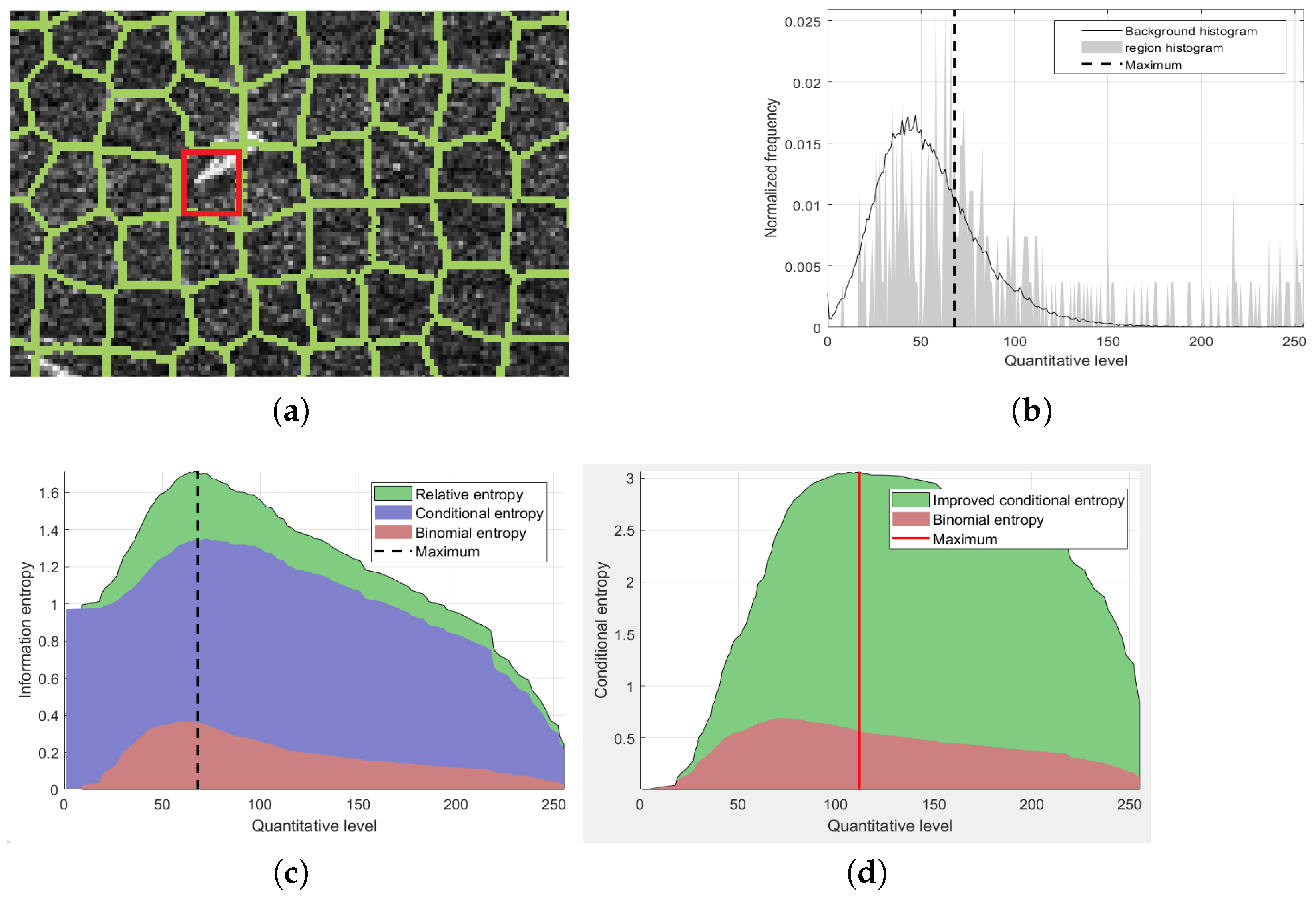
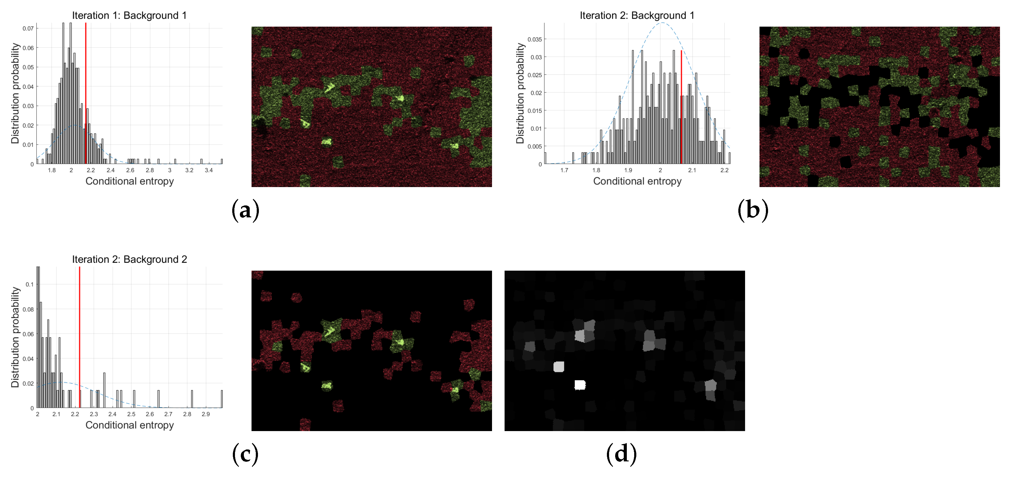
In order to further analyze the change law of the two functions, the values of the above equation are calculated for the target super-pixel shown in the red box in Figure 2a. The brighter pixels in the region belong to the target, while the rest of them are backgrounds. In Figure 2b, the gray area shows the normalized histogram of this area, and the black curve shows the normalized histogram of the whole SAR image. The horizontal axis quantitative level means 256 gray scales. Therefore, Figure 2b shows the frequency of pixels in each gray level. In Figure 2c, the horizontal axis is the value of l k , while the vertical axis is the corresponding conditional entropy, h k , and the sum of them. When l k is the quantization level on the leftmost side of the horizontal axis, the corresponding ordinate value is the relative entropy. With the increase of l k , it can be seen that both conditional entropy and h k will increase at first but then decrease, and the maximum value of the sum is reached from the position shown by the vertical line in Figure 2c.
Besides, it can be shown from Equation (8) that when K n | R n | / 2 , h k reaches the maximum value, which means that this item will potentially make the target pixels close to the number of background pixels. Reflected in the figure, the position of the maximum value in the red area represents that the proportion of target and background is the same. In Figure 2c, this position is very close to the maximum position (the vertical line), indicating that the maximum position is also close to K n | R n | / 2 . However, in Figure 2a, in the red box, the target area is significantly less than the background areas. Therefore, this result is inaccurate. In fact, in the normal image region, the pixel proportion of the target and the background are rarely equal. Thus, the binomial entropy h k , which is independent of the target, can be ignored. This section proposes an improved model for conditional entropy. The result is shown in the Figure 2d.
Firstly, the conditional entropy is simplified by referring to the method in literature [20], the number of quantization levels that satisfying the condition H n ( l ; K n ) > 0 and l l k are set as q. So we can substitute H n ( l ; K n ) = 1 / q for the original conditional entropy, and ignore the effect of l o g ( 1 / q ) . At the same time, the coefficient K n / | R n | of the original conditional entropy has a strong constraint on its value, which results in K n approaching | R n | . Therefore, we add the logarithmic term log ( | R n | / K n ) as the coefficient. The final improved conditional entropy model is shown as (9):
D ( H P 0 ; K n ) = K n | R n | log | R n | K n H n ( l ; K n ) > 0 1 q · log P 0 ( l )
The improved conditional entropy is still a function of l k or K n . Similar to the analysis of the relative entropy, K n is taken as a parameter to calculate the maximum value of the improved condition entropy, and the corresponding K ^ n is obtained as:
K ^ n = arg max K n D ( H P 0 ; K n )
K ^ n is taken as the Maximum Likelihood Estimation (MLE) [29,30] result of the number of target pixels, and the maximum value is defined as D ( H n ; K ^ n ) . This value will maximize the LRT of the target superpixel.
In the experiment of the same superpixels in Figure 2a, the value of the improved conditional entropy is shown in Figure 2d. The quantization level corresponding to the maximum value is shown by the red vertical line. Compared with the position of the maximum value in Figure 2c, K ^ n is more shifted to the right side, that is, less than | R n | / 2 , which is closer to the real proportion of the target pixel in the super-pixel region.
In order to make the description simple, the conditional entropy in the following refers to the function D ( H n ; K ^ n ) . For the scattering features of superpixel region, the proposed piece-wise histogram takes into account the mixing of target and background, which is more consistent with the actual situation, and the scattering features of the target and the background are further enhanced.

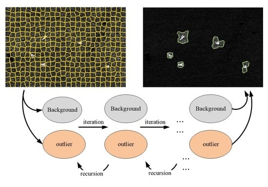
2.2. Iterative Outlier Detection

Although the conditional entropy of superpixels can be directly applied to discriminate targets and backgrounds, the detection effect is affected by two factors: the selection of detection threshold and background region. The former determines the detection performance, while the latter is related to the measure of conditional entropy and the accuracy of detection. The problem is that the prior information of both is usually unknown. In order to improve the adaptability of the detection algorithm, iterating outlier detection is proposed in this section. In each iteration, the background region is adjusted according to the last detection result, and the relative detection threshold also changes due to the change of background, so the results of multiple iterations can realize an effective background selection and detection threshold design.
Generally speaking, most of the superpixels in SAR images belong to the background, while there are only a small number of target superpixels. When the background is a uniform ground scene, and its scattering also satisfies the homogeneity assumption, then the overall background region and the local background superpixel have similar scattering statistical features. Based on these two assumptions, the conditional entropy of most of the superpixels in SAR image also satisfies the similarity, while only a small number of background and target superpixels do not have the similarity. These special pixels are called outliers. Therefore, a simple statistical outlier detection method is adopted, which centers on the mean value of all the superpixel conditional entropy and expresses the deviation degree by its standard deviation. The detection process of outliers is as follows:
(1) Select the background area and use its histogram to calculate the conditional entropy D ( H n ; K ^ n ) ;
(2) Calculate the sample mean μ h and variance σ h 2 of conditional entropy in this set;
μ h = 1 N D ( H n ; K ^ n ) σ h 2 = 1 N 1 ( D ( H n ; K ^ n ) μ h ) 2
(3) Normalize the conditional entropy;
D ( H n ; K ^ n ) = D ( H n ; K ^ n ) μ h σ h
(4) Detect outliers based on threshold t 0 .
D ( H n ; K ^ n ) t 0
A suitable threshold t 0 is set to distinguish background from outliers. When the left side of the above equation is greater than or equal to t 0 , the n -th superpixel is considered to be an outlier, otherwise it belongs to the background.
In general, single outlier detection has the advantages of simplicity and high efficiency, but it may face two difficulties when detecting complex high-resolution SAR images: (1) when the imaging region contains multiple types of ground objects, the superpixels of different scenes may cause the center of conditional entropy deviation. Because of this problem, some superpixels of the scene will be detected as outliers, forming a large number of false alarms; (2) The variance of conditional entropy of superpixels in complex scenes are larger, which leads to the decrease of conditional entropy after standardization.It is easy to cause missing detection.
In some CFAR detection algorithms [31,32], the iterative method is used to optimize the selection of background pixels. In these methods, with the increase of iterations, a growing number of pixels are detected as targets and excluded from the background area. This process gradually improves the accuracy of background estimation and helps to improve the detection effect. Therefore, for the background selection problem of single outlier detection, the iterative strategy is also applied.
Specifically, at the beginning of the iteration, the background may contain complex scenes and some target superpixels. Although the influence of them on the histogram may be small, the background area is still changed after detecting the partial segregating group value by the empirical threshold. In the subsequent iterations, the set of background superpixels will be gradually divided into outliers and background. The expected stop conditions will be achieved, until the maximum number of iterations, or when the number of new outliers is less than the set value.
We adopt the superposition strategy to realize iterative detection, that is, to assign label b n to the superpixel. In the iteration, the label of the outlier is superimposed. Let the initial background be the set of all superpixels: { R 0 } . The superscript indicates that the initial labels of the superpixels is all 0. In iterative detection, superpixels with the same label belong to the same background set, Outlier detection is performed on each set respectively, and the label of outlier superpixels is updated:
b n i + 1 = b n i + 1 , D 0 i ( H n ; K ^ n ) t 0 b n i , D 0 i ( H n ; K ^ n ) < t 0
where t 0 is used to achieve the division of background and outliers.
The label of the outlier increases by 1, indicating that the superpixel is added to the background set corresponding to the next label. Conversely, the label of the background superpixel remains the same. In addition, the label of any superpixel does not exceed the current iteration number i. Then, an iteration is completed after detecting outliers and updating the label for the background set with labels 0 to i 1 , respectively.
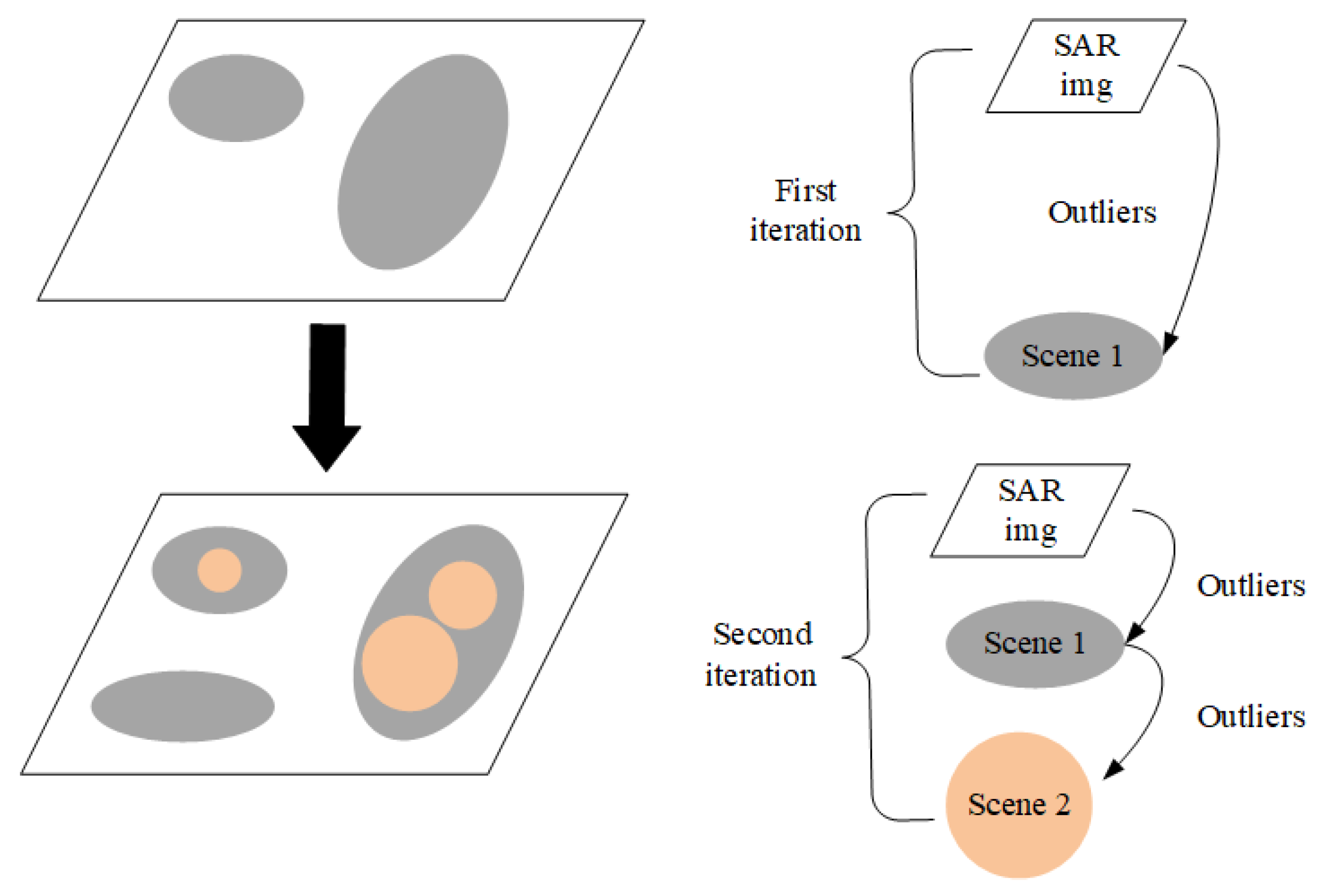
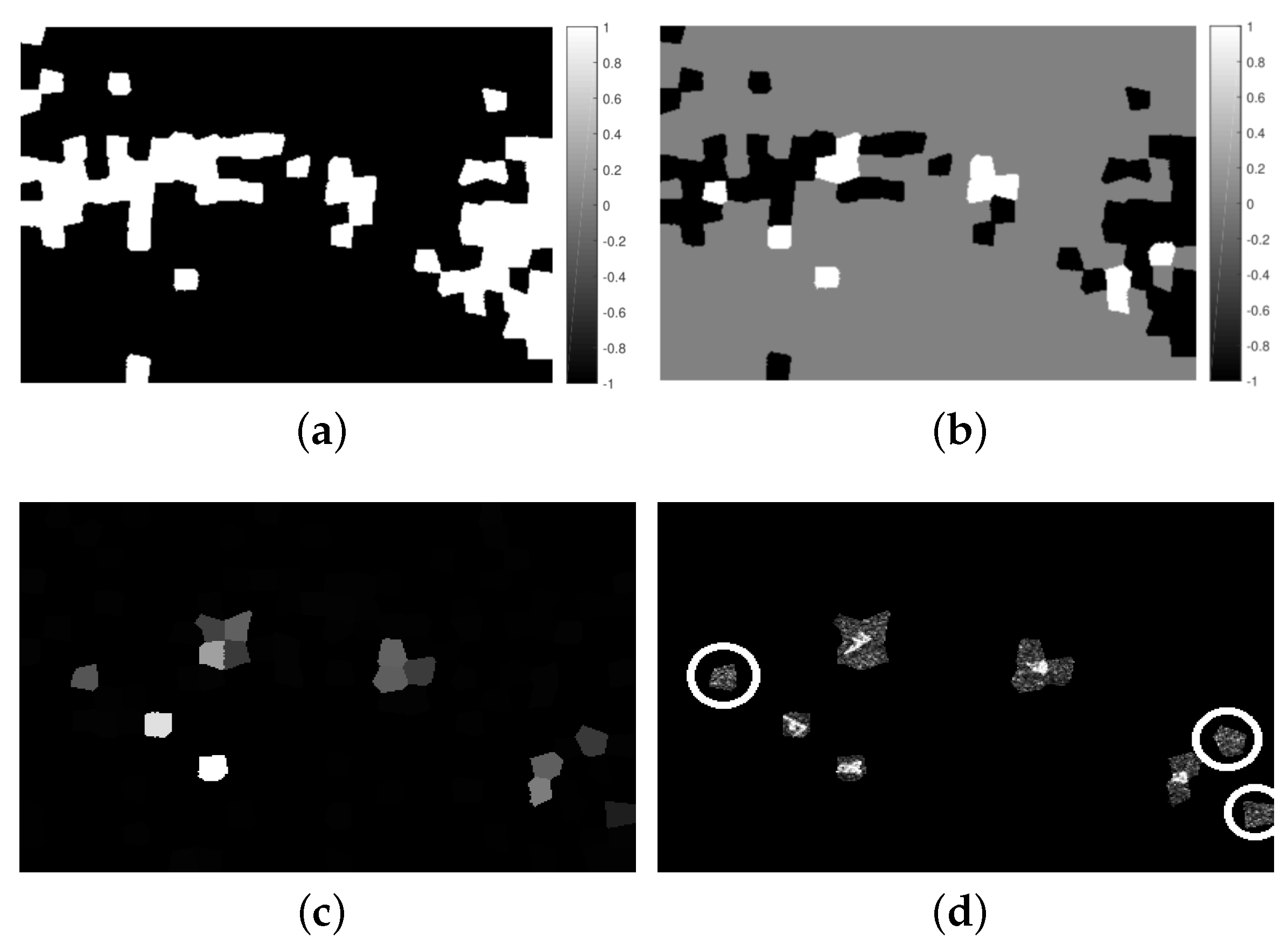
A simple example of two iterations is shown in Figure 3. In the first iteration, the whole SAR image is taken as the background. As indicated in the brackets on the right, we use the white parallelogram to represent the whole SAR image. The detected outliers called Scene 1 are shown as the gray area (two gray ellipses) in the first parallelogram. In the second iteration, the region outside Scene 1 in the SAR image is taken as a background set. The outliers detected again are shown by the third gray ellipse in the lower left corner of the second quadrangle. Then, taking the corresponding area of Scene 1 as another background set, outliers are detected, as shown in the orange circles below the arrow. In the second iteration, when the outlier label is updated, ellipse in the the lower left corner of the right side is added to Scene 1. Then, the circles in ellipses are updated to Scene 2. Repeat the above process to achieve iterative outlier detection, we need to pay attention to update the outlier labels after finishing detection of each scene, so as to avoid changing the background set in a single iteration.
It can be seen from the above recursive method that the iterative detection based on superposition strategy has the following features:
(1) After outliers are detected and labeled, the complexity of background set is reduced;
(2) Adding outliers as a new background set is equivalent to a smaller outlier detection problem;
(3) After the superpixels of the target are detected as outliers for many times, their labels overlay is higher, which makes them more saliency than the background. Therefore, the superposition of superpixel outlier degree can be provided as a saliency for subsequent steps.
By continuously adjusting the division of background set, the uniform background region in SAR image is gradually screened out, which improves the accuracy of background selection.

2.3. Recursing Saliency Depth

Outliers reflect the superpixels which differ from the background. The more different the superpixels are, the more attention we will pay. Therefore, in the iterative process, when the background and outliers vary wildly, it is generally considered that the corresponding scene is more likely to contain the target of interest. S. Liu proposed the concept of saliency depth to evaluate the possibility of targets in multi-class scenes [27]. The method in this subsection does not use scene classification in detection, but represents different scenes through iterative detection of background set, so it can also use saliency depth analysis to analyze the possibility of target existence.
In this section, the saliency of outliers in iteration is evaluated by the saliency depth of recursion. The high saliency outliers are retained, and the low saliency superpixels are suppressed to achieve saliency correction.
First, calculate the degree of deviation of outliers in the scene, denoted as initial salience:
S 0 = 1 Ω o = 1 Ω | ξ o t 0 | 3 1 3
where Ω is the number of outlier superpixels, ξ o is the regional features measure of outliers after standardized processing, such as self information or conditional entropy. ξ o t 0 represents the degree of outlier deviating from the threshold. In the initial saliency S 0 , we want to highlight the outliers far from the threshold. Therefore, we use power 3 to deal with the degree of outlier. The experiment of S. Liu [27] shows that the scene containing targets has higher initial saliency, while for the pure background SAR image with Equivalent Number of Looks (ENL, a parameter commonly used to measure the speckle suppression of different SAR/OCT image filters) greater than 1, its initial saliency is often smaller.
After excluding the current outlier in the scene, the outlier is detected again and the salience is calculated using Equation (15), which is called the predicted salience S p . If some salient targets in the scene are not detected as outliers, the prediction saliency may be high, which means that the background area needs to be further detected and divided. On the other hand, assuming that all salient targets have been included in the outliers, after excluding the outliers, the saliency of the background superpixel set is lower than the initial case, which means that further detection of the background region may be unnecessary.
In the experiment, it is found that the prediction saliency of the non-target scene itself may also be higher than the initial saliency. In order to calculate the saliency depth, we set S p = β S p , β = 0.75 to widen the gap between the initial value and the predicted value. Finally, the depth of salience is defined as Δ S = S 0 S p . These two values measure the complexity of the background set, while depth indicates whether outlier detection is effective in reducing the complexity of the background.
The saliency depth requires the calculation of two salience, and the difference between the two is determined by outlier screening. The saliency depth of iterative detection is calculated by the following equation:
Δ b i S = S b i β S b i + 1 , i = 1 , , I 1
where Δ b i S represents the saliency depth of the set labeled b in the i-th iteration, and S b i represents the initial salience of the set. In addition, the initial salience corresponding to all labels and number of iterations can be combined into matrix S R I × I , where the rows represent number of iterations and the columns represent number of labels; Δ S is the result of row difference of matrix S . This step is called recursing saliency depth, because it uses the salience provided by the next iteration.
From Equation (16), if Δ S is large, it means that the background superpixel after outlier screening has uniformity and does not need to be further detected; otherwise, it means that the background set after outlier screening has little difference from the previous background set, which may have been a pure background or there is a target to be detected. Therefore, we need to find the maximum value for each column of the matrix Δ S :
Δ ^ b S = max i = 1 , , I 1 Δ b i S
The background of label b reaches its maximum depth of salience at iteration i ^ b .
In order to optimize the detection results, the effective outliers in different backgrounds should be enhanced, and the effective background regions should be suppressed to generate a reasonable global salience map. We proposed a fusion method based on saliency depth. Firstly, the outlier degree and background corresponding to the maximum saliency depth are used for enhancement and suppression, respectively:
S a l n b = + i ^ b Δ ^ b S , b n i ^ + 1 > b n i ^ = b i ^ b Δ ^ b S , b n i ^ + 1 = b n i ^ = b
In the i ^ b -th iteration, the set of label b corresponds to the maximum saliency depth, and the salience value of the outlier is positive i ^ b Δ ^ b S , whereas the salience value of the background is equal to its negative value. Then, combining with the salience value of the outlier itself, that is, adding the loss item of Hinge, the final salience value S a l n is obtained:
S a l n = i = 1 I L n i + b = 0 I 1 S a l n b
where L n i is the Hinge loss term with a positive value. In order to avoid missed detection, for the superpixel with positive salience value, its mean salience value μ s and standard deviation σ s are used for global detection:
μ s = 1 N + S a l n > 0 S a l n , σ s = 1 N + S a l n > 0 ( S a l n μ s ) 2
where N + is the total number of positive outliers.
Then, the empirically selected global detection threshold t g = μ s + σ s is used to determine whether the superpixel belongs to the potential target or background:
T n = True , S a l n t g False , S a l n < t g
If T n is true, it indicates that the n-th superpixel is the potential target region, otherwise, it belongs to the background region.
However, in order to avoid missed detection, the outlier threshold and global detection threshold are usually set with very small value, so there are still a few false alarms. When the target pixel proportion is very low, it will result in the loss of target information. To solve the above problems, local information is used to optimize the detection results.

2.4. Local Salience Optimization

The arrangement of the centers of superpixels is usually irregular, so it is necessary to build a graph model with superpixels as nodes, and make local access through the edges of adjacent superpixels. When a node has a short path to a background (target) seed node, then this node is also classified as a background (target).
Considering the complexity of calculation, a graph model is established only for the local neighborhood of each potential target superpixel, denoted as G = V , E , where V = V n 1 M is the set of M superpixel nodes. The adjacency matrix E = [ e m n ] M × M represents the M × M edges. Since only adjacent superpixels have effective edges, the edge weight is calculated by the following equation:
e m n = D ( V m , V n ) , n N ( m ) + , n N ( m )
where N ( m ) is the node set adjacent to the m-th node, and the edge weight between adjacent nodes is D ( V m , V n ) , the edge weight between disconnected nodes is infinite. In addition, the edge of the superpixel is made to satisfy symmetry, that is, e m n = e n m .
In order to detect the target superpixels that the conditional entropy cannot distinguish and filter out the false alarm, the KS (Kolmogorov-Smirnov) test value is calculated only by using the first K non-zero gray levels in the adjacent superpixels:
D K S ( m , n ) = sup l = 1 , , K F m ( l ) F n ( l )
where F m ( · ) is the CDF (Cumulative Distribution Function) of the first K gray levels of the m-th superpixel, and F m ( 1 ) = 0 , F m ( K ) = 1 . KS test is similar to conditional entropy in that it restricts strongly scattered pixels, but KS test has symmetry, so it is more in line with local detection requirements.
For the target split into adjacent superpixels, the centroid of mass of strongly scattered pixels in superpixel is extracted. In the adjacent background superpixel, the distance between the centroid of mass is long, but in the adjacent target superpixel, the distance is short. Therefore, we calculate the euclidean distance D C ( m , n ) of the centroid of mass of strong scattering in the adjacent superpixel and introduce it into the edge weight:
e m n = D K S ( m , n ) · D C ( m , n )
Then, the potential target superpixels in the global detection results are taken as the target seeds, and the rest are the background seeds. At the same time, the potential target superpixels are sorted according to the salience value, and the target seeds with high salience value are given priority for local detection. q is used to represent the ordinal number of the potential target superpixel after sorting, which satisfies the following order inequality:
S a l 1 S a l q S a l Q > μ s
Therefore, when local detection is carried out on the q-th superpixel, its adjacent node set N q = { V p | e p q + } is checked. When N q contains only the potential target, we can appropriately expand the scope of its neighborhood until it includes the background seed. When N q only contains the background, a virtual target seed can be assumed: its histogram is replaced by the average histogram of the first q target seeds, and then the distance between V q and KS is calculated. The distance between V q and its center of mass is replaced by the maximum distance from the pixel to its own center of mass in the superpixel V q . N q is used to build the local graph model, and the weights of the middle edges are assigned.
According to the distance between V q and N q , the nodes with the shortest distance are assigned to V q to achieve local detection. After Q potential targets are processed in order of salience value from high to low, local salience optimization is completed.

3. Experiment

In order to verify our target detection algorithm, experiments and analysis are carried out from three aspects: (1) Simulated SAR images are used for testing to demonstrate the functions of our method; (2) Several SAR images are tested to verify the detection performance of the method in this chapter for different scenes; (3) Compared with CFAR and WIE method, the features and advantages of our method is analyzed. Each experiment will be described in detail below.

3.1. Testing Process Experiment

A simulated SAR image for testing is shown in Figure 4a, with a uniform grass background and a size of 384 × 256 . The target embedded in the background comes from the public data set “Moving and Stationary Target Acquisition and Recognition” (MSTAR). There are five targets to be detected, and the resolution radio of each is 0.3 m × 0.3 m. The radar works in X-band and the polarization mode used is HH polarization mode. Firstly, the size parameter W { 16 , 32 } is set to analyze the influence of this parameter on the regional scattering features model. The two sizes of superpixels are shown in Figure 4b,c, respectively. As shown in the figure, the size of the target is closer to 16 × 16 pixels, but some targets are still split into multiple regions because of the deviation of superpixels’ centers. While choosing the size 32 × 32 , the target superpixels contain a large number of background pixels. The pixel proportion of the target and background in the superpixels vary with their size, so it can be inferred that there are also differences in the regional histogram. Then, three kinds of information measures are calculated respectively: self information, relative entropy and conditional entropy. The outlier detection threshold t 0 is set as 0.8. The outlier degree of superpixel obtained is shown in Figure 4b,c.
As shown in Figure 4, the three information entropy measures are less affected by the size of superpixels, but there are differences among superpixels with different target pixel proportions. As shown more clearly in Figure 4b, for most target superpixels, the outlier degree of self information and conditional entropy is very close. However, the relative entropy outlier degree of intermediate target is weaker than the other two measures, as shown by the white circle in the second row. In addition, although the degree of outlier of some backgrounds is highlighted through the lower threshold, and the degree of outlier of the uniform background is still generally small, there are several obvious background superpixels in the self information and relative entropy results, as shown in the white box in Figure 4b. Compared with the SAR image, the background superpixels with high degree of outlier belong to the shadow area. It is speculated to be caused by the utilization of all gray levels in the regional histogram by self information and relative entropy. On the contrary, the conditional entropy with strong scattering gray as the parameter does not have this problem, which is more conducive to target detection.
Then, continue the experiment on the method with W = 16 in Figure 4a, and analyze the effect of iterative detection and recursive processing. However, the background of the simulated SAR image is uniform grassland, the satisfactory detection effect can be achieved after two iterations. Therefore, set the maximum number of iterations I = 2 , and the threshold of outlier detection is t 0 = 1.2 by default. However, in order to highlight more outliers for comparison of detection effects, t 0 = 0.6 is selected in this experiment. The conditional entropy distribution, outlier detection results and iterative accumulation results of Hinge loss in the iteration are shown in Figure 5. The left half of Figure 5a shows the conditional entropy distribution histogram of superpixels at the first iteration. Background 1 includes the whole image, in which the red vertical line identifies the outlier detection threshold. The right side of the histogram is the corresponding outlier division result. The red area is the background and the green area is the outlier. Similarly, Figure 5b,c show the conditional entropy distribution and outlier detection results of the second iteration, and in the second iteration, background 1 is composed of the background region of the detection results of the first iteration, while background 2 is composed of the outlier region of the first detection results.
Due to the low threshold t 0 , the outliers detected for the first time include the target and part of the background. For simple scene images, false alarms can be filtered by increasing the threshold, but it is very difficult to select the empirical threshold for complex SAR images. Thus, in the second iteration, although the threshold is still low, the outlier detection of background 2 has saliently reduced the number of false alarm superpixels, as shown in the green area in Figure 5c. The results show that multiple iterative detection is similar to gradually adjusting the detection threshold. In the second iteration, the detection result of background 1 contains many outliers, and all are background superpixels. However, from the conditional entropy distribution in the left half of Figure 5b, it can be seen that the maximum distance from these outliers to the threshold is about 0.15 (the outlier is about 1.85 while the threshold is about 2), which is far less than the maximum degree of outliers detected in the other two outliers. In addition, the degree of outlier Hinge loss of each super-pixel in the two iterations is accumulated to obtain the results shown in Figure 5d. In the figure, the target has been highlighted from the background area, but there are still some dark background areas need to be further processed.
The initial saliency is calculated based on the conditional entropy distribution in Figure 5a–c. In the first iteration, some superpixels are far from the threshold, and the saliency of background 1 is 0.2804. Similarly, in the second iteration, the saliency of background 1 is 0.0555 and the saliency of background 2 is 0.2488. Therefore, the saliency depth of the first iteration is 0.2388, which means that background 1 has achieved good results in the first outlier detection, and the second detection may be redundant. Therefore, the results of Figure 5a,c are used for saliency depth fusion by the method of Equation (18) in Section 2.4. For simplicity, take the positive saliency correction value + i ^ b Δ ^ b S as +1 while the negative one is set as −1 in the schematic diagram. It can be seen that the area of +1 in Figure 6a cancels the area of −1 in Figure 6b, but the area of +1 in both is enhanced. The recursive saliency depth fusion results are shown in Figure 6c. Compared with the Hinge fusion results in Figure 6d, it is found that the saliency of most background areas is worth suppressing.
The detection result based on the global threshold t g is shown in Figure 6d, which contains three background superpixels as shown in a white circle, and its formation reason is still the deliberately set threshold t 0 = 0.6 . Using the default threshold t 0 = 1.2 can eliminate false alarms, but the local graph model detection can also achieve the same effect. Figure 7a shows the difference of the shortest distance between the superpixel and the background seed and the target seed in the local neighborhood. The area without local detection is displayed as 0. When the superpixel is more similar to the background, the distance difference is negative, as shown in the darker area in the figure. On the contrary, the distance difference of the superpixel more similar to the target is positive and displayed as a brighter area. Figure 7b shows the final detection result after local optimization. It can be seen that the false alarm in the global detection result is suppressed and the target area is retained. The results of the above processes verify the feasibility of the method proposed in this section.

3.2. Experiment in Complex Scenes

We tested our method in real complex situations. The experimental parameters are set as: t 0 = 1.2 , I = 4 , the predictive salience coefficient β = 0.75 , and K = 30 in the local detection.
Figure 8 shows two high-resolution airborne SAR images based on self owned and cooperative SAR systems, but the scene complexity is different. The resolution of them is 0.5 m × 0.5 m with full polarization model and X-band. The first one shows the real SAR image of the land scene, in which the complexity of the background is high. There is amplitude attenuation on the left and right sides of the image. The white circles in the figure identify the vehicle targets. The iterative detection results are shown in Figure 8b. The results after recursive processing and local optimization are shown in Figure 8c–e.
The background of the latter image is a uniform airport area, targeting three aircraft and other small ground objects. The SAR image of the aircraft is composed of many strong scattering centers. Similarly, the iterative detection results are shown in Figure 8b, while the results after recursive processing and local optimization are shown in Figure 8c–e.
The above experiments show that taking the superpixel as the standard, the detection rate of the main targets in the test image is 100%, and the number of false alarm superpixels is 0.

3.3. Methods Contrast Experiment

We chose two detection methods for comparative analysis: CFAR detection based on G 0 distribution and WIE detection based on weighted information entropy. However, the detection rate and false alarm rate of these three methods are calculated in different ways, a unified quantitative index cannot be obtained, so the effect can only be evaluated intuitively.
In Figure 9, SAR images from top to bottom are labeled as images 1–4, detection results of the four SAR images are shown successively in Figure 9b–d. Our parameter settings are consistent with experiment 1; The false alarm rate of CFAR detection for image 1 is set as 0.001, and in image 2–4 is set as 0.01. The density filtering threshold of CFAR is set as 10 pixels, which means that the target detection results with local density less than 10 pixels are screened out. The false alarm rate of WIE is set to be the same as that of CFAR to ensure the detection effect. Under the condition of ensuring the detection effect, the outlier detection threshold is set empirically within the interval [ 0.2 , 2 ] .
The detection results of four SAR images by the comparison method are shown in Figure 9b–d. The CFAR results are the target pixel binary maps, while the results of WIE and our method are the target region. Image 1 is a SAR image measured by ourselves with a resolution of 0.5 m × 0.5 m. There are five tanks models in the image and the background is uniform grass. Image 2 is a SAR image of the simulated complex scene with a resolution of 0.3 m × 0.3 m, which comes form MSTAR data set. The radars of image 1 and 2 work in X-band and the polarization mode used is HH polarization mode. Image 3 is a self owned image with X-band and HH polarization mode. There are also three vehicle targets in image 3 with a resolution of 1 m × 1 m. Image 4 is a SAR image containing ocean and land scenes with 11 ship targets on the sea. It comes from the Canadian radar satellite RADARSAT-1. Its resolution is 8 m × 8 m, C-band and polarization mode is HH. In image 3 and 4, the size of the target is small and the scattering is weaker than that of the land scene, so self-information is used to replace conditional entropy for iteration and recursion.
In order to further quantitatively compare various methods, we selected 30 images from MSTAR public data set and high-resolution airborne SAR images for statistics. Considering the differences between images, we set t 0 = 1.2 , I = 4 to simplify the parameter adjustment process as much as possible. For the size of superpixels, as the size of a image is L × H , L H , we set W = H / 32 . For comparison, the other three methods we choose are CFAR detection based on G 0 distribution, WIE detection based on weighted information entropy and conditional entropy algorithm without iteration. The results are shown in Table 1.

4. Discussion

This method mainly verifies the feasibility of each link, the detection effect under the background of different complexity and the advantages compared with other methods through Testing process experiment, Experiment in complex scenes and Methods Contrast experiment. Next, each experiment will be analyzed one by one.

4.1. Testing Process Experiment

Due to the need for a large number of reference to the result images of each link for discussion, the analysis results of testing process experiment have been described in the previous article. In conclusion, from experiment 3.1, we can see that the steps of experimental design effectively improve the detection effect, and finally get a good result. Therefore, the results of each process verify the feasibility of our method.

4.2. Experiment in Complex Scenes

The main test objects of this experiment are two high-resolution SAR images with different background complexity, target shape and scattering features. Comparing the two test images in Figure 8, we can find that the scattering of vehicle targets circled by white circles in the first image is not as obvious as that of the aircrafts in the following image. In Figure 8b, The high degree of outliers in the background region reflects its complexity. However, the results after recursive processing and local optimization are still improved, as shown in Figure 8c–e.
For the second image, as we can see, the superpixel does not fully fit the complex shape of the aircraft, and contains some surrounding background pixels. However, the strong scattering of aircraft target forms a high significant value, so it can be detected correctly. Although some small targets shown in the white circle in Figure 8d can be detected globally, they are filtered out in the local results in Figure 8e. It indicates that the small targets are more similar to their surrounding background. Detecting smaller targets requires reducing the superpixel size.
From the detection results of the test images, although the background complexity, target shape parameters and scattering features of the two images are different, they have achieved good detection performance, which proves the effectiveness and universality of this method for SAR images.

4.3. Methods Contrast Experiment

In Figure 9, we can compare the advantages and disadvantages of CFAR, WIE, and our method. In image 1, all the targets are detected by all three methods. Although the number of false alarm pixels in CFAR results is 0, the target area detected by CFAR is fractured. In the WIE result, the segmentation of the target area is complete, but there are two false alarms, as shown in the white box in the first line of Figure 9c. The algorithm proposed by us can also extract the target region completely. Although the superpixel size is larger than the target, so that the target region contains background pixels, the number of independent false alarm is 0.
In image 2, the three methods can also detect three vehicle targets correctly. Outside the target area, CFAR detection generates a large number of false alarm pixels. Compared with image 2 in Figure 9a, it is found that the false alarm is mainly composed of tree canopy and ground artificial objects. The result of WIE showed that there are 5 false alarm areas, which were formed by the canopy of strong scattering. There are also four false alarm areas in our method, but they are mainly ground artificial objects.
There are also three vehicle targets in image 3 just like image 2, but the background scattering intensity is much greater than that in image 2. The results of CFAR and WIE produce a large number of false alarm pixels or regions, while it can be seen that our method correctly detects the target superpixels with only one false alarm area. Comprehensive comparison shows that our method is better than the two comparison methods.
In image 4, the size of the target ship is smaller and the scattering is weaker than that in the land area. Therefore, in order to avoid missed detection, set the outlier detection threshold t 0 = 0 , that is, superpixels with self information greater than the mean value are considered outliers. In CFAR result, there are a large number of false alarms at the junction of land and sea, while there are serious omissions in WIE result. In the result of our method, all targets are detected correctly with only a small number of false alarm superpixels.
From Table 1, although the effect is not so good on individual images, our method has obvious advantages in detection rate and false alarm rate compared with the other three methods. To sum up, through reasonable parameter setting, our method can achieve effective target detection in SAR images and achieve better detection results than other methods. However, for SAR images with different complexity, some parameters still need to be selected empirically. In addition, our method still produced a lot of false alarms for some images, which needs to be further improved through deep-going research. To solve this problem, our next research interests should be to fuse more features and improve the detection accuracy through multiple discrimination. Another solution is to process the image in advance through dimension reduction or denoising to reduce redundant information, which cannot only assist detection, but also reduce the amount of calculation.

4.4. Techniques for Target and Change Detection

Remote sensing change detection is to quantitatively analyze and determine the features and process of land surface change from remote sensing data in different periods, which means that it usually needs to process a large amount of data. The traditional frequency decomposition methods include Fourier transform, least square spectral analysis and their correction. With the improvement of the accuracy of remote sensing data, random noise makes the observation values show more uncertainty. With the rapid increase of data volume, computational complexity optimization has become another major challenge for time series analysis in dealing with large data sets. At present, the popular methods such as short-time Fourier and wavelet transforms, Hilbert-Huang transform, constrained least squares spectral analysis and least squares wavelet analysis have their own advantages and disadvantages in dealing with these two challenges [33]. The Least-Squares Cross-Spectral Analysis is a method of analyzing multiple time series together, which get good results by multiplying the Least-Squares Spectra of both time series [34]. Another solution idea is to reduce redundant information by means of data compression and denoising data, such as dimension reduction. A processing pipeline was proposed to compress hyper-spectral images both spatially and spectrally before applying target detection algorithms to the resultant scene in [35]. The experimental results show that the pipeline can compress more than 90% of the data and maintain the target detection performance [35]. For satellite remote sensing images, our method improves the effect of background selection by iterating outliers, and can achieve good detection effect. Therefore, in terms of detecting the changes in such images, our method can improve the discrimination effect between background and targets, reduce the false rate, and accumulate prior knowledge to identify targets such as vehicles and ships more accurately.

5. Conclusions

Based on the idea of segmentation before detection, an improved target detection method via iterative outliers and recursive significant depth was proposed by us and compared with other methods to verify the effectiveness and superiority of this method. This method mainly had four stages. At first, the superpixel of the target usually also contained background pixels after superpixel segmentation. In view of this phenomenon, we used the number of target pixels as a parameter to establish a piece-wise function model of regional scattering statistical features, and putted forward the conditional entropy measure. Experiments showed that the conditional entropy based on this model was more suitable for target detection than other information entropy. It overcame the influence of target and background pixel mixing on detection. Secondly, for complex SAR images, different scene regions could cause background histogram deviation, which also made the conditional entropy measure inaccurate. In this regard, we further used the iterative outlier detection strategy to realize the background selection. Then, we used the recursive saliency depth to correct the redundant outliers in the iterative process. Compared with the traditional single detection without iteration, it achieved better detection effect for complex scene images. Finally, because missed detection was avoided when setting the threshold, some false alarms were usually included in the global detection results. Combined with the local features of the target superpixel, we designed the local saliency optimization. The experiment results verified that this step could effectively suppress the false alarm and preserve the target area. In the experimental part, compared with the other SAR image target detection algorithms, our method achieved more accurate detection results for a variety of scenes or target types. For SAR images with large scene differences, although our method could achieve good detection results, some parameters still needed to be selected empirically, such as outlier detection threshold, number of iterations and so on. Our method improves the background selection and detection threshold design through iteration, but it still does not completely solve this problem. Therefore, automatic target detection should be deeply studied in the follow-up work.

Author Contributions

Conceptualization, Z.C. (Zongyong Cui); Data curation, Y.Q. and Y.Z.; Formal analysis, Z.C. (Zongyong Cui); Funding acquisition, Z.C. (Zongyong Cui) and Z.C. (Zongjie Cao); Investigation, Y.Q.; Methodology, Y.Q.; Project administration, Z.C. (Zongyong Cui); Resources, Z.C. (Zongyong Cui); Software, H.Y.; Supervision, Z.C. (Zongyong Cui) and Z.C. (Zongjie Cao); Writing—original draft, Y.Q. and Y.Z. All authors have read and agreed to the published version of the manuscript.

Funding

This work was supported by Science and Technology on Automatic Target Recognition Laboratory (ATR) Fund 6142503190201, and the National Natural Science Foundation of China under Grant 61971101 and 61801098.

Institutional Review Board Statement

Not applicable.

Informed Consent Statement

Not applicable.

Data Availability Statement

Some images used in this paper come from “Moving and Stationary Target Acquisition and Recognition” (MSTAR). The others are self owned data unpublished.

Acknowledgments

We sincerely appreciate the three anonymous reviewers for improving this manuscript.

Conflicts of Interest

The authors declare no conflict of interest.

Abbreviations

CDFCumulative Distribution Function
CFARConstant False Alarm Rate
ENLEquivalent Number of Looks
GLRTGeneralized Likelihood Ratio Test
KSKolmogorov-Smirnov
LRTLikelihood Ratio Test
MLEMaximum Likelihood Estimation
MSTARMoving and Stationary Target Acquisition and Recognition
PDProbability of Detection
PFAProbability of False Alarm
RISHrotation invariant symbol histogram
SARSynthetic Aperture Radar
SCRSignal Clutter Ratio
SLICSimple Linear Iterative Cluster
SNRSignal-to-Noise Ratio
WIEWeighted Information Entropy

References

  1. El-Darymli, K.; McGuire, P.; Power, D.; Moloney, C. Target detection in synthetic aperture radar imagery: A state-of-the-art survey. J. Appl. Remote Sens. 2013, 7, 071598. [Google Scholar] [CrossRef] [Green Version]
  2. Harris, B.W.; Milo, M.W.; Roan, M.J. Symbolic target detection in SAR imagery via rotationally invariant-weighted feature extraction. Int. J. Remote Sens. 2013, 34, 8724–8740. [Google Scholar] [CrossRef]
  3. Liu, B.; Chang, W.; Li, X. A Novel Range-spread Target Detection Algorithm Based on Waveform Entropy for Missile-borne Radar. In Proceedings of the International Conference on Advances in Satellite and Space Communications, Think Mind, Venice, Italy, 21–26 April 2013; pp. 46–51. [Google Scholar]
  4. Wang, Q.; Zhu, H.; Wu, W.; Zhao, H.; Yuan, N. Inshore Ship Detection Using High-Resolution Synthetic Aperture Radar Images Based on Maximally Stable Extremal Region. J. Appl. Remote Sens. 2015, 9, 095094. [Google Scholar] [CrossRef]
  5. Liang, C.; Wang, C.; Bi, F.; Li, C. A new region growing based method for ship detection in high-resolution SAR images. In Proceedings of the Iet International Radar Conference, Hangzhou, China, 14–16 October 2015; p. 5. [Google Scholar] [CrossRef]
  6. Li, T.; Liu, Z.; Ran, L.; Xie, R. Target Detection by Exploiting Superpixel-Level Statistical Dissimilarity for SAR Imagery. IEEE Geosci. Remote Sens. Lett. 2018, 15, 562–566. [Google Scholar] [CrossRef]
  7. Stutz, D.; Hermans, A.; Leibe, B. Superpixels: An Evaluation of the State-of-the-Art. Comput. Vis. Image Underst. 2016, 166, 1–27. [Google Scholar] [CrossRef] [Green Version]
  8. Yue, Z.; Zou, H.; Luo, T.; Qin, X.; Zhou, S.; Ji, K. A Fast Superpixel Segmentation Algorithm for PolSAR Images Based on Edge Refinement and Revised Wishart Distance. Sensors 2016, 16, 1687. [Google Scholar] [CrossRef] [Green Version]
  9. Arisoy, S.; Kayabol, K. Mixture-Based Superpixel Segmentation and Classification of SAR Images. IEEE Geosci. Remote Sens. Lett. 2016, 13, 1721–1725. [Google Scholar] [CrossRef]
  10. Feng, J.; Pi, Y.; Yang, J. SAR image superpixels by minimizing a statistical model and ratio of mean intensity based energy. In Proceedings of the IEEE International Conference on Communications Workshops, Budapest, Hungary, 9–13 June 2013; pp. 916–920. [Google Scholar] [CrossRef]
  11. Xiang, D.; Ban, Y.; Wang, W.; Su, Y. Adaptive Superpixel Generation for Polarimetric SAR Images With Local Iterative Clustering and SIRV Model. IEEE Trans. Geosci. Remote Sens. 2017, 55, 3115–3131. [Google Scholar] [CrossRef]
  12. Liu, N.; Cao, Z.; Cui, Z.; Pi, Y.; Dang, S. Multi-Scale Proposal Generation for Ship Detection in SAR Images. Remote Sens. 2019, 11, 526. [Google Scholar] [CrossRef] [Green Version]
  13. Wang, Y.; Liu, H. PolSAR Ship Detection Based on Superpixel-Level Scattering Mechanism Distribution Features. IEEE Geosci. Remote Sens. Lett. 2015, 12, 1780–1784. [Google Scholar] [CrossRef]
  14. He, J.; Wang, Y.; Liu, H.; Wang, N.; Wang, J. A Novel Automatic PolSAR Ship Detection Method Based on Superpixel-Level Local Information Measurement. IEEE Geosci. Remote Sens. Lett. 2018, 15, 384–388. [Google Scholar] [CrossRef]
  15. Odysseas, P.; Alin, A.; David, B. Superpixel-Level CFAR Detectors for Ship Detection in SAR Imagery. IEEE Geosci. Remote Sens. Lett. 2018, 15, 1397–1401. [Google Scholar] [CrossRef] [Green Version]
  16. Yu, W.; Wang, Y.; Liu, H.; He, J. Superpixel-Based CFAR Target Detection for High-Resolution SAR Images. IEEE Geosci. Remote Sens. Lett. 2016, 13, 730–734. [Google Scholar] [CrossRef]
  17. Cheng, M.; Mitra, N.J.; Huang, X.; Torr, P.H.S.; Hu, S. Global Contrast Based Salient Region Detection. IEEE Trans. Pattern Anal. Mach. Intell. 2015, 37, 569–582. [Google Scholar] [CrossRef] [PubMed] [Green Version]
  18. Jiang, B.; Zhang, L.; Lu, H.; Yang, C.; Yang, M. Saliency Detection via Absorbing Markov Chain. In Proceedings of the 2013 IEEE International Conference on Computer Vision, Sydney, Australia, 1–8 December 2013; pp. 1665–1672. [Google Scholar] [CrossRef] [Green Version]
  19. Zhai, L.; Li, Y.; Su, Y. Inshore Ship Detection via Saliency and Context Information in High-Resolution SAR Images. IEEE Geosci. Remote Sens. Lett. 2016, 13, 1870–1874. [Google Scholar] [CrossRef]
  20. Liu, S.; Cao, Z.; Yang, H. Information Theory-Based Target Detection for High-Resolution SAR Image. IEEE Geosci. Remote Sens. Lett. 2016, 13, 404–408. [Google Scholar] [CrossRef]
  21. Li, T.; Liu, Z.; Xie, R.; Ran, L. An Improved Superpixel-Level CFAR Detection Method for Ship Targets in High-Resolution SAR Images. IEEE J. Sel. Top. Appl. Earth Obs. Remote Sens. 2018, 11, 184–194. [Google Scholar] [CrossRef]
  22. Huo, W.; Huang, Y.; Pei, J.; Qian, Z.; Qin, G.; Yang, J. Ship Detection from Ocean SAR Image Based on Local Contrast Variance Weighted Information Entropy. Sensors 2018, 18, 1196. [Google Scholar] [CrossRef] [PubMed] [Green Version]
  23. Ma, F.; Gao, F.; Sun, J.; Zhou, H.; Hussain, A. Attention Graph Convolution Network for Image Segmentation in Big SAR Imagery Data. Remote Sens. 2019, 11, 2586. [Google Scholar] [CrossRef] [Green Version]
  24. Zhang, J.; Feng, H.; Luo, Q.; Li, Y.; Li, J. Oil Spill Detection in Quad-Polarimetric SAR Images Using an Advanced Convolutional Neural Network Based on SuperPixel Model. Remote Sens. 2020, 12, 944. [Google Scholar] [CrossRef] [Green Version]
  25. Sun, Z.; Liu, M.; Liu, P.; Li, J.; Yu, T.; Gu, X.; Yang, J.; Mi, X.; Cao, W.; Zhang, Z. SAR Image Classification Using Fully Connected Conditional Random Fields Combined with Deep Learning and Superpixel Boundary Constraint. Remote Sens. 2021, 13, 271. [Google Scholar] [CrossRef]
  26. Li, Y.; Xing, R.; Jiao, L.; Chen, Y.; Chai, Y.; Marturi, N.; Shang, R. Semi-Supervised PolSAR Image Classification Based on Self-Training and Superpixels. Remote Sens. 2019, 11, 1933. [Google Scholar] [CrossRef] [Green Version]
  27. Liu, S.; Cao, Z.; Wu, H.; Pi, Y.; Yang, H. Target detection in complex scene of SAR image based on existence probability. Eurasip J. Adv. Signal Process. 2016, 2016, 114. [Google Scholar] [CrossRef] [Green Version]
  28. Achanta, R.; Shaji, A.; Smith, K.; Lucchi, A.; Fua, P.; Süsstrunk, S. SLIC Superpixels Compared to State-of-the-Art Superpixel Methods. IEEE Trans. Pattern Anal. Mach. Intell. 2012, 34, 2274–2282. [Google Scholar] [CrossRef] [PubMed] [Green Version]
  29. Potter, L.C.; Moses, R.L. Attributed scattering centers for SAR ATR. Image Process. IEEE Trans. 1997, 6, 79–91. [Google Scholar] [CrossRef] [Green Version]
  30. Ding, B.; Wen, G.; Huang, X.; Ma, C.; Yang, X. Data Augmentation by Multilevel Reconstruction Using Attributed Scattering Center for SAR Target Recognition. IEEE Geosci. Remote Sens. Lett. 2017, 14, 979–983. [Google Scholar] [CrossRef]
  31. An, W.; Xie, C.; Yuan, X. An Improved Iterative Censoring Scheme for CFAR Ship Detection With SAR Imagery. IEEE Trans. Geosci. Remote Sens. 2014, 52, 4585–4595. [Google Scholar] [CrossRef]
  32. Cui, Y.; Zhou, G.; Yang, J.; Yamaguchi, Y. On the Iterative Censoring for Target Detection in SAR Images. Geosci. Remote Sens. Lett. IEEE 2011, 8, 641–645. [Google Scholar] [CrossRef]
  33. Ghaderpour, E.; Pagiatakis, S.D.; Hassan, Q.K. A Survey on Change Detection and Time Series Analysis with Applications. Appl. Sci. 2021, 11, 6141. [Google Scholar] [CrossRef]
  34. Ghaderpour, E.; Ince, E.S.; Pagiatakis, S.D. Least-squares cross-wavelet analysis and its applications in geophysical time series. J. Geod. 2018, 92, 1223–1236. [Google Scholar] [CrossRef]
  35. Macfarlane, F.; Murray, P.; Marshall, S.; White, H. Investigating the Effects of a Combined Spatial and Spectral Dimensionality Reduction Approach for Aerial Hyperspectral Target Detection Applications. Remote Sens. 2021, 13, 1647. [Google Scholar] [CrossRef]
Figure 1. Target detection flow chart based on iteration and recursion.
Remotesensing 13 04315 g001
Figure 2. Conditional entropy of SAR image region. (a) Select area, (b) Normalized histogram of region and background, (c) Relative entropy, conditional entropy and binomial entropy of K n , (d) Improved conditional entropy.
Remotesensing 13 04315 g002
Figure 3. An example of iterative outlier detection.
Remotesensing 13 04315 g003
Figure 4. Outlier detection of different size superpixels. (a) Simulation of SAR image, and superpixel segmentation results when size parameters W = 16 and W = 32 ; (b) The outlier degree of self information, relative entropy and conditional entropy of with W = 16 ; (c) The outlier degree of self information, relative entropy and conditional entropy with W = 32 .
Remotesensing 13 04315 g004
Figure 5. Two iterative simulation SAR image detection results. (a) Conditional entropy distribution and outlier detection in the first iteration; (b) In the second iteration, the conditional entropy distribution and outlier detection of background 1; (c) In the second iteration, the conditional entropy distribution and outlier detection of background 2; (d) Iterative accumulation results of Hinge loss.
Remotesensing 13 04315 g005
Figure 6. The correction amount and recursive result of simulated SAR image. (a) Correction amount of background 1; (b) Correction amount of background 2; (c) Saliency recursive results; (d) Global detection results.
Remotesensing 13 04315 g006
Figure 7. Local graph model detection. (a) The difference of the shortest distance from the superpixel to the background seed and the target seed; (b) Partial detection result.
Remotesensing 13 04315 g007
Figure 8. (a) Original SAR image; (b) Iterate the outlier degree; (c) The results of the recursive correction; (d) The results of global detection; (e) The results of local optimization.
Remotesensing 13 04315 g008
Figure 9. Comparison of SAR image target detection results. (a) Original SAR image; (b) G 0 -CFAR; (c) WIE; (d) Our algorithm.
Remotesensing 13 04315 g009
Table 1. Comparison of SAR image target detection results.
ItemReal TargetDetected TargetFalse TargetDetection RateFalse Alarm Rate
Method
G 0 -CFAR16314511988.3%45.1%
WIE16314110686.5%42.9%
single detection16315010692.0%41.4%
Our algorithm1631566995.7%30.7%
Publisher’s Note: MDPI stays neutral with regard to jurisdictional claims in published maps and institutional affiliations.

