1. Introduction
Recently, near-field 3-D synthetic aperture radar (SAR) imaging and its applications have become an important research direction [
1,
2,
3]. When SAR imaging results are displayed in 3-D form, the occlusion caused by the background (the sidelobes, noise, and interference) makes the main lobe difficult to observe. The target extraction of a 3-D SAR image is an efficient algorithm for eliminating the influence of the background. Scholars are committed to investigating the target extraction algorithm with high accuracy and computational efficiency. For target extraction, the image segmentation method is usually utilized to divide the image into several categories, and then the target is determined through certain judgment conditions.
In computer vision, medicine, and other fields, image segmentation methods based on fuzzy C-means (FCM) and hidden Markov random fields (HMRF) are widely used due to their good performance. Recently, researchers have been working hard to improve the performance of these two types of algorithms [
4,
5,
6,
7,
8]. One of the main means of improvement is the introduction of information into neighboring voxels to improve the anti-noise ability [
9,
10,
11].
We try to use general segmentation algorithms to complete the target extraction of 3-D SAR images. However, when these algorithms are applied to 3-D SAR images, it is difficult for them to avoid the influence of interference whose intensity is very close to the target. As a result, some strong interference voxels are incorrectly divided into the target voxels. In addition, some segmentation algorithms tend to use more complex objective functions to obtain better anti-noise ability. And these algorithms are usually designed for the processing of 2-D images. When these algorithms are applied to 3-D images, the complex objective functions make their computational efficiency unacceptable. Therefore, most of the algorithms that exist are not suitable for direct application to the segmentation of 3-D SAR images.
A 3-D SAR image has sparsity [
12], which means that the number of background voxels in a 3-D SAR image is far higher than that of target voxels. We consider the region where the target is located as the region of interest (ROI). If one algorithm can be applied to remove the background area with the interference and extract ROI, then the high-performance image segmentation algorithm only needs to divide the voxels in ROI. This not only improves the anti-interference ability but also the computational efficiency.
The region-adaptive morphological reconstruction fuzzy C-means (R-AMRFCM) algorithm [
13] is an ROI-based algorithm specifically designed for 3D SAR image target extraction. It utilizes the anisotropic diffusion method [
14] to smooth the image, the 3-D Kirsch method to calculate the gradient magnitude, and the hysteresis threshold method to extract target edges. The minimum bounding polyhedrons of the target edges are regarded as the ROI. The adaptive morphological reconstruction fuzzy C-means algorithm was then used to divide the target voxels and the background voxels in ROI. However, R-AMRFCM has two disadvantages:
The gradient threshold in the anisotropic diffusion filter and the two thresholds in the hysteresis threshold method have to be adjusted manually. The adjustment process is experience-dependent and time-consuming;
The target extraction of different images in one data set is achieved by the same thresholds. These thresholds are not optimal for each image.
In this paper, we will focus on designing an ROI-based preprocessing algorithm which can obtain the required thresholds adaptively in order to make general segmentation algorithms suitable for 3-D SAR image target extraction. Image features can reflect the unique information contained in each image, and different images have different features. If a mapping relationship can be established between the required thresholds and image features, the thresholds can be calculated adaptively. Thereby, we aim to find a way to achieve ROI extraction with an adaptive threshold.
There are some statistical models that fit the distribution of gray levels in SAR images; these include Gamma distribution, Gamma mixture distribution (GMD), generalized Gamma distribution (GGD), etc. [
15,
16,
17,
18,
19,
20,
21,
22]. The gray levels of the 3-D SAR images that we processed [
13,
23,
24] follow Gamma distribution. Furthermore, the algorithm proposed in this paper is based on this hypothesis. The histogram is an important feature for SAR images. Researchers have achieved a variety of SAR image applications through histograms [
25,
26,
27,
28]. For example, Qin et al. proposed a classification algorithm and a segmentation algorithm for SAR images based on GGD [
29,
30]. Pappas et al. proposed a framework to extract a river area from a SAR image based on GGD [
31]. Xiong et al. presented a change detection measure based on the statistical distribution of SAR intensity images [
32]. Therefore, we also utilize the histogram to achieve an ROI extraction with an adaptive threshold.
In this paper, an ROI extraction algorithm with adaptive threshold (REAT) is proposed to improve the anti-interference ability and the computational efficiency of existing segmentation algorithms. Firstly, a fast saliency detection algorithm is applied to enhance the 3-D SAR image [
33]. Secondly, the features of the original image and the enhanced image (the image mean, the histogram, etc.) are obtained. Based on the histograms of the original image and the enhanced image, the Kullback–Leibler distance (KLD) is utilized to evaluate the difference between these two images. Otsu’s method [
34] is used to calculate the reference thresholds. Subsequently, the gradient threshold in the anisotropic diffusion method is calculated with the histogram and the image mean. Two thresholds in the Canny edge detection method [
35] are calculated with the use of the reference thresholds and the KLD. Then, the anisotropic diffusion method is employed to smooth the image, and the Canny edge detection method is applied to extract the target edges. Finally, the minimum bounding cuboids of the target edges are considered as the core region, and the boundary of the core region is expanded outward to form a buffer area. The core region and the buffer area constitute a complete ROI. Moreover, the expansion reduces the loss of target regions caused by inaccurate edge extraction.
The extracted ROI can be directly treated as the input of the existing image segmentation algorithms. In this paper, a Gaussian-based hidden Markov random field and some FCM-based segmentation algorithms are utilized to divide the target voxels and the background voxels in ROI.
Our contribution is summarized as follows:
Designed for 3-D SAR images, we propose a preprocessing algorithm to quickly extract the region of interest. The proposed algorithm can improve the performance and efficiency of general image segmentation algorithms. Moreover, the proposed algorithm is flexible and can easily be applied to existing image segmentation methods;
The image features are utilized to adaptively obtain the thresholds required for ROI extraction. The thresholds are independently optimized for different images.
The rest of this paper is organized as follows. In
Section 2, we review related works. In
Section 4, the theory of the proposed algorithm is described.
Section 5 introduces the experimental results and the performance evaluations. In
Section 6, we illustrate the process of the proposed algorithm and discuss the role of the buffer area. The conclusion is given in
Section 7.
3. Background
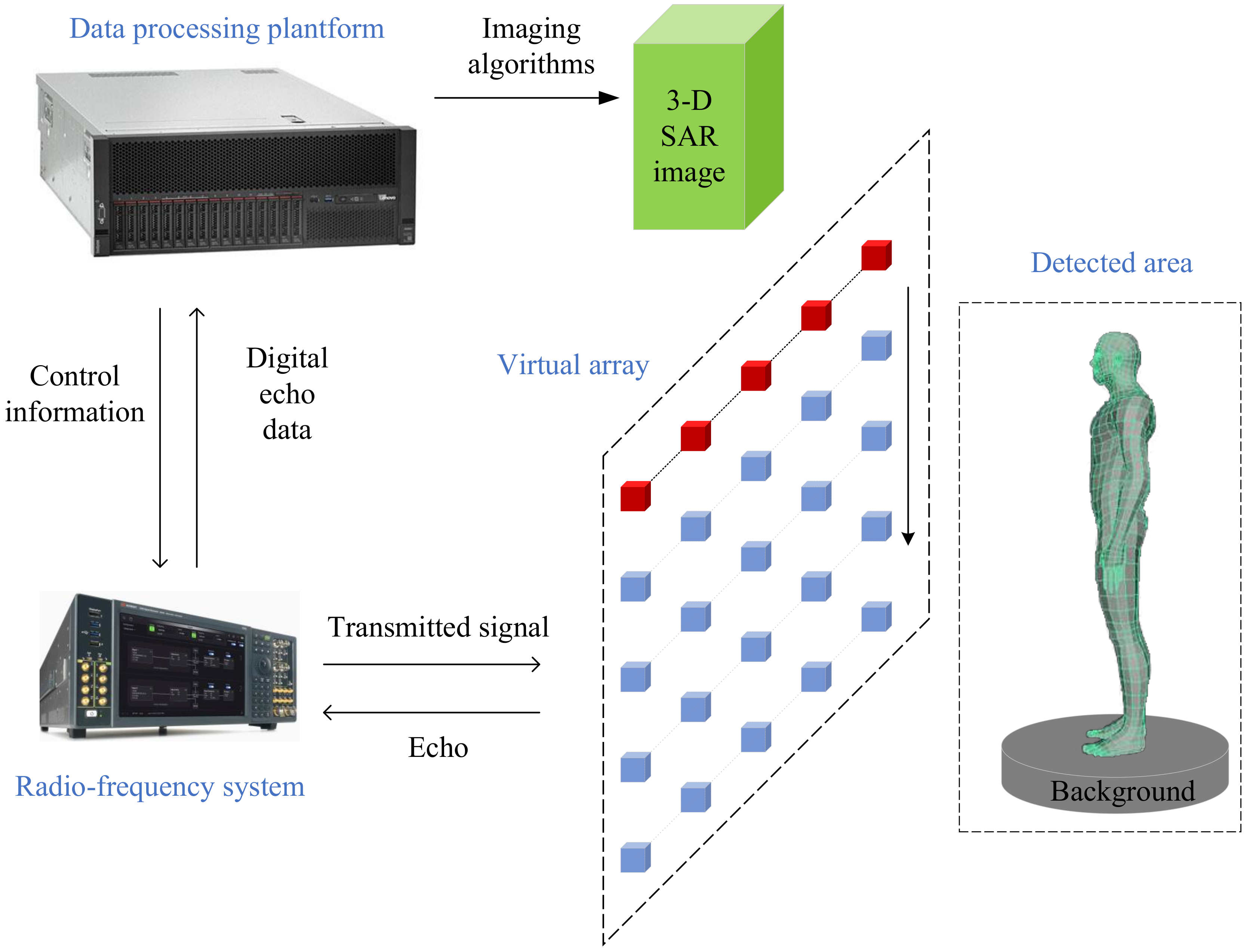
The 3-D SAR imaging system for security inspection usually consists of three main parts: a virtual array, a radio frequency system (RFS) for transmitting signals and collecting echoes, and a data processing platform (DPP) for storing the digital echo data and imaging. And the framework of the 3-D SAR imaging system for security inspection is shown in
Figure 1. The SAR system uses wideband signals and matched filtering to obtain range resolution. In order to obtain the resolution of the other two dimensions (cross-track direction and along-track direction), a virtual array is generated on a plane perpendicular to the distance direction. For the security inspection SAR imaging system, a 1-D real antenna array is usually used to generate a virtual array. This mode takes into account the cost and scanning time.
The DPP sends the control information to the RFS. Then, the RFS transmits signals and receives echoes through antennas. After the analog-to-digital conversion, the digital echo data is transmitted from the RFS to the DPP. Finally, the DPP stores the digital echo data and achieves 3-D SAR imaging. References [
23,
24] show two different near-field 3-D SAR imaging systems.
The 3-D SAR image can be divided into two parts: target and background. There are some high-intensity interferences in the background, and the intensity of these interferences is almost equal to the intensity of the weak target. For general image segmentation algorithms, it is difficult to distinguish between weak targets and strong interferences based on intensity alone. Reference [
13] shows that the edge gradient intensity of the target is usually stronger than that of the interference. Therefore, the target and the interference can be distinguished by the difference in edge gradient intensity. This paper designs an ROI extraction algorithm based on this idea.
4. Method
Influenced by interference, general image segmentation algorithms are not suitable for the target extraction of 3-D SAR images. Therefore, we propose an ROI extraction algorithm with adaptive threshold (REAT) to enhance the anti-interference ability and computational efficiency of general image segmentation algorithms. The input of REAT is a 3-D gray scale voxel image, and its output is one or more small-sized 3-D gray scale images (regions of interest). For near-field 3-D SAR images, voxels with higher gray levels tend to be judged as target voxels. When designing REAT, the area gathered by voxels with higher gray levels is judged as the region of interest. In this section, we will elaborate on the inspiration and theory of the proposed algorithm.
4.1. Overview
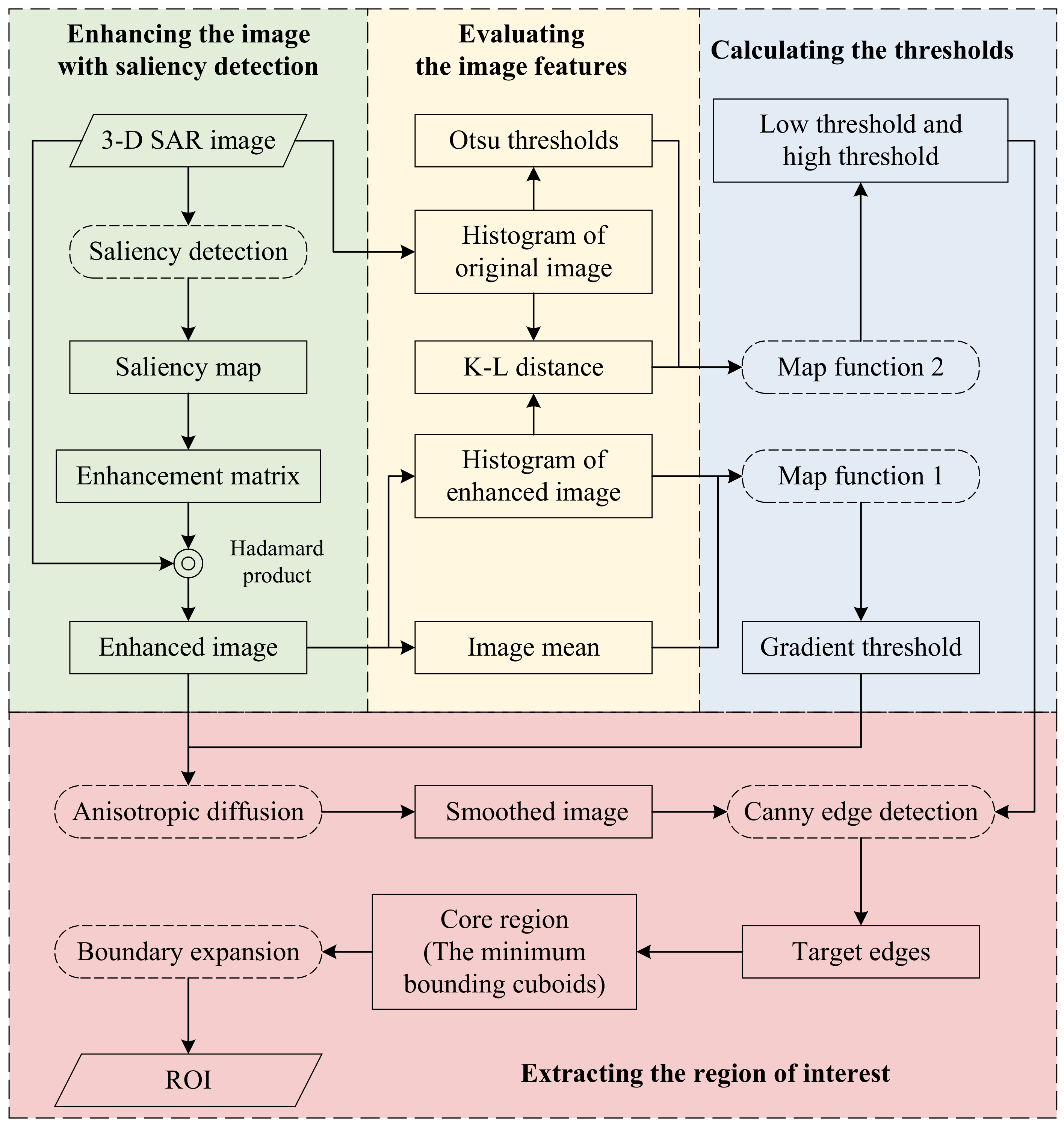
The proposed algorithm consists of 4 main steps, and the structure is shown in
Figure 2. Firstly, the saliency map of the original image is calculated by the spectral residual method. Based on the saliency map, the enhancement matrix is generated. The saliency-enhanced image is calculated by the Hadamard product of the original image and the enhancement matrix. Secondly, the mean value of the enhanced image, the histogram of the enhanced image, and the histogram of the original image are calculated. In addition, two reference thresholds are calculated by Otsu’s method based on the histogram of the original. After calculating the probability distribution function of the original image and the enhanced image with the histogram, the Kullback–Leibler distance between these two images is obtained. Then, the gradient threshold of the anisotropic diffusion algorithm and the thresholds of the Canny edge detection algorithm are calculated by two map functions with the above-mentioned results. Finally, after smoothing the enhanced image with the anisotropic diffusion algorithm, the Canny algorithm is used to detect the target edges. The minimum bounding cuboids of the target edges are regarded as the core region. After expanding the boundary of the cuboids outwards, the expanded area is then considered the buffer area. The core region and buffer area constitute the complete ROI.
We introduce the proposed algorithm in detail in the following subsections.
4.2. Image Enhanced by Saliency Detection
Assuming that the matrix of the gray levels of the original image is
,
is the element in
,
,
,
. The set of gray levels of all voxels is
,
. The spectral residual method is applied to calculate the saliency map
of
.
is the gray-level normalized result of
. Then, the enhancement matrix is constructed as follows:
where
denotes the gain,
denotes a matrix whose elements are all 1. The enhanced image
is expressed as:
where ⊙ denotes the Hadamard product. Image saliency enhancement reduces the intensity of the background area. We will illustrate this in
Section 6.1.
4.3. The Calculation of the Gradient Threshold
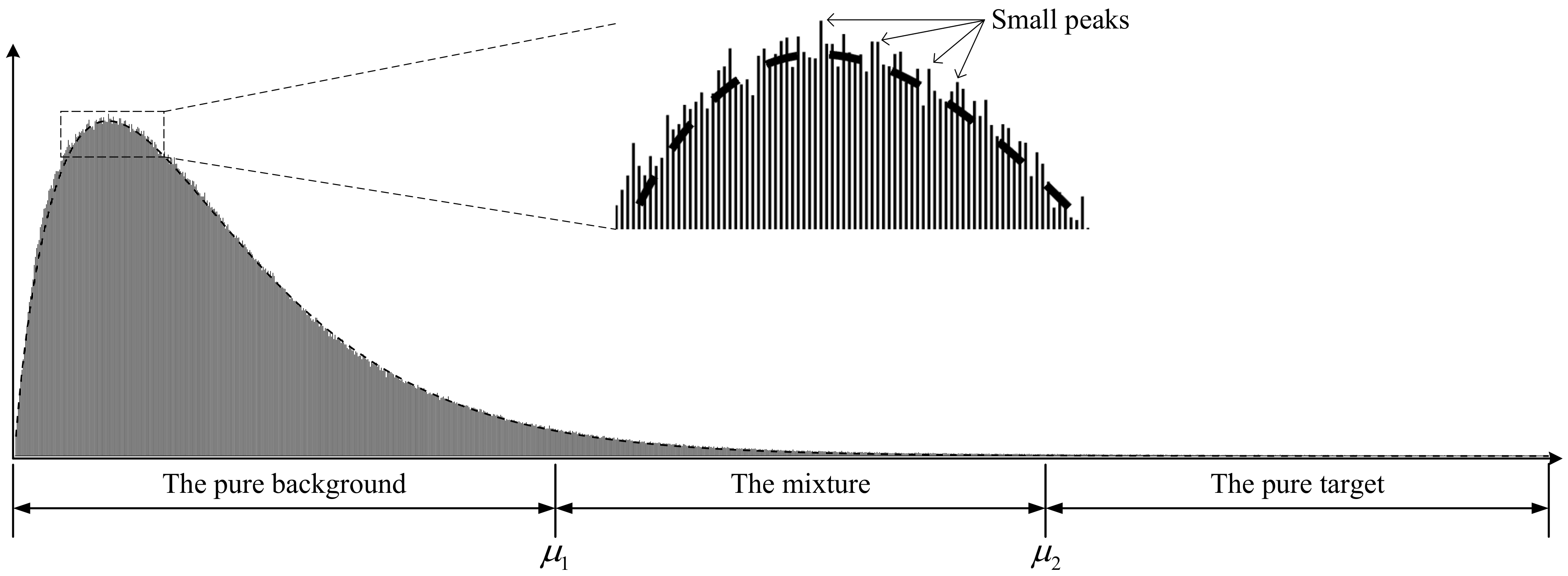
In this paper, assume that a 3-D SAR image follows the Gamma distribution. The schematic of a 3-D SAR image histogram is shown in
Figure 3. For near-field SAR detection, the target usually has high intensity. Due to the sparsity of 3-D SAR images, the number of background voxels with low gray levels is much higher than the number of target voxels with high gray levels. Thus, there is a serious imbalance between the number of target voxels and the number of background voxels. In addition, the histogram is not a smooth curve, and there are many small peaks on the histogram.
The gradient threshold in the anisotropic diffusion algorithm depends on the noise level and edge strength [
14]. In this paper, the gradient threshold is regarded as the boundary between the target and the background. According to the histogram, the huge peak in the low gray-level range is almost contributed by the background. If the gray level with the largest number of voxels is regarded as the median of the background intensity, two times the median of the background intensity can be roughly regarded as the boundary between target and background. However, this boundary is unstable and susceptible to small peaks. To improve the stability of the boundary, the mean value of
gray levels with the largest number of voxels is taken as the median of the background intensity. The larger the
, the more stable the median of the background intensity. However, because the histogram of the Gamma distribution is asymmetric, too large an
will cause the offset of the median of the background intensity. Empirically,
is set to 5.
The calculation of the median of the background intensity only considers the image background information and ignores the target information. We believe that the gradient threshold should be calculated after a complete evaluation of the image. Therefore, the image mean that includes both background information and target information is introduced to correct the threshold calculated before.
The set of gray levels of the enhanced image is
, and the mean value of the image is
is
. The histograms of the original image and the enhanced image are
and
, respectively;
. Both histograms have the same gray level
. The histogram of the enhanced image is sorted from largest to smallest. The sorted histogram is
, where the gray level corresponding to
is
. Hence, the median of the background intensity is
. The gradient threshold
is calculated with the following map function:
So far, we have obtained the gradient threshold for the anisotropic diffusion algorithm.
4.4. Canny Edge Detection and the Calculation of Two Thresholds
According to the distribution of voxels in the histogram, it is inferred that there is a threshold so that the voxels whose gray level is in the range of are part of the background. Similarly, there is a threshold so that the voxels whose gray level is higher than are targets. Thus, these two thresholds divide the histogram into three intervals: the pure background, the mixture of the target and the background, and the pure target.
According to the threshold , the histogram is divided into two regions. The voxels belonging to the pure background are directly discarded. The voxels belonging to the mixture and the pure target are extracted and considered as the ROI. This allows for a large number of background voxels to be removed.
There is some strong interference in the 3-D SAR image. These interference voxels are usually distributed in the pure background and the mixture. If the ROI and the background are roughly divided by the threshold
, the interference voxels in the mixture will be divided into the ROI at the same time. In addition, these interference voxels seriously influence the segmentation result. Reference [
13] pointed out that there is a difference between the edge gradient magnitude of the target and the interference, which can be used to eliminate the influence of the interference. According to this idea, the Canny edge detection method is applied to extract the target edges while eliminating the interference. The minimum bounding cuboids of the target edges after boundary expansion also forms the ROI. Among them,
and
correspond to the low threshold and the high threshold, respectively. In this way, ROI extraction not only removes the voxels in the pure background, but also eliminates the interference voxels in the mixture. The difficulty of image segmentation is greatly decreased.
Otsu’s method [
34] is an efficient histogram-based method of calculating the reference thresholds. However, the imbalance in the number of voxels between the background and the target makes the reference thresholds inaccurate. Therefore, the imbalance needs to be corrected. For the images before and after the saliency enhancement, there are differences in the background and target information between these two images. Moreover, the Kullback–Leibler distance can measure these differences. Therefore, we utilize the Kullback–Leibler distance to evaluate these differences and use the evaluation result to correct the reference thresholds. The map function is used to achieve further adjustment.
Assuming that the reference thresholds calculated by Otsu’s method are
and
, respectively, and
. The probability distribution of the original image
and the probability distribution of the enhanced image
are calculated with the corresponding histogram, respectively:
The Kullback–Leibler distance between the original image and the enhanced image is expressed as follows:
The thresholds after correction are expressed as follows:
The range of and are . is usually a small value.
If
and
are directly regarded as the low threshold and the high threshold, when
is much smaller than
, some interference edges will be regarded as the target edges. Hence, the power function is introduced to narrow the gap between these two thresholds. However, the power function increases the values of
and
at the same time. The coefficient
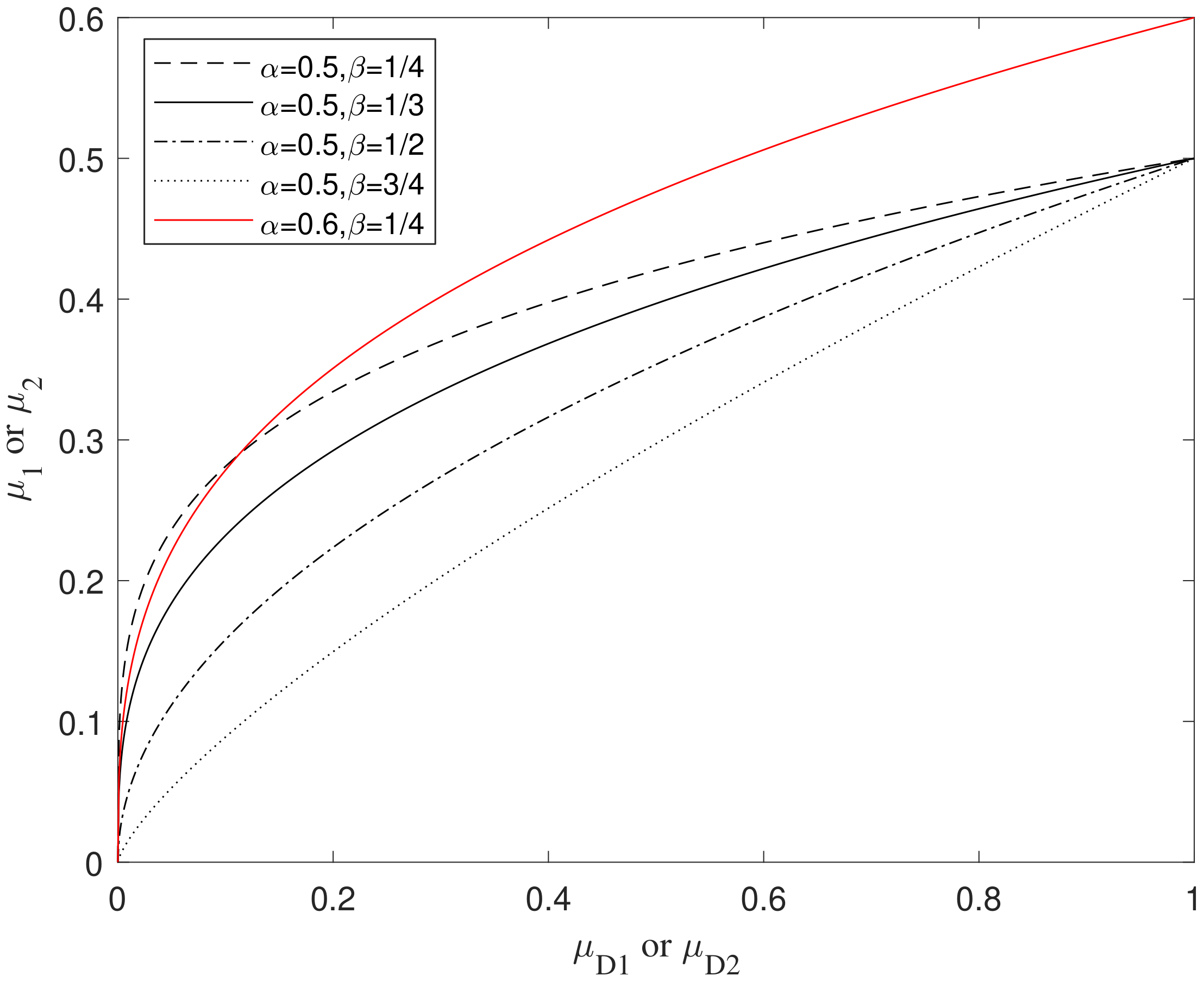
is thus introduced to offset the negative effects of the power function. The map function is constructed as follows:
where
and
are the coefficients.
Figure 4 shows the relationship between these two coefficients and the map function in the range of
. The value with
is mapped to the value with
. The smaller the coefficient
, the smaller the gap between
and
. In this paper,
and
are set to 0.5 and
, respectively.
4.5. The Extraction of ROI and Target
The thresholds required by the anisotropic diffusion method and the Canny edge detection algorithm have been calculated. After smoothing the enhanced image with the anisotropic diffusion method, the Canny algorithm is applied to extract the target edges. Thus, several regions formed by the minimum bounding cuboids of the target edges are determined, and the set of these regions is regarded as the core region. The inaccurate edge detection causes the permanent loss of part of the target region. Therefore, we expand the boundary of the core region outward to the voxels. The expanded area is named the buffer area. The core region and the buffer area form the complete ROI , . The next step is to accurately divide the voxels in each region through an image segmentation method.
Each region is composed of target voxels and background voxels, , where denotes the set of target voxels in the wth region, and denotes the set of background voxels in the wth region. G-HMRF is used to achieve the division of voxels in each region . The category containing the highest gray-level voxels is marked as the target, and the other category is marked as the background. Thereby, the union of all target voxel sets is extracted. To decrease over-segmentation, the voxels whose gray level is less than are regarded as background and removed. To improve the accuracy, the times upsampling is performed on each region before image segmentation, and the region size is restored after the image segmentation is completed.
5. Experiments
5.1. Evaluation Criterion
Accuracy, precision, recall, and the dice similarity coefficient (DSC) were used to evaluate the performance of the target extraction algorithm. denotes the whole image. denotes the extracted target region. denotes the ground truth.
Accuracy represents the ratio of the number of voxels correctly classified to the number of total voxels in the image:
Precision represents the ratio of the number of correctly extracted target voxels to the number of all extracted target voxels:
Recall represents the ratio of the number of correctly extracted target voxels to the number of real target voxels:
The dice similarity coefficient, also known as the
-score, indicates the similarity between the correctly extracted target region and the real target region:
The value range of the four criteria above is . The closer the value is to 1, the better the performance is. Among them, the DSC is the most important because of its comprehensive evaluation ability.
5.2. Experimental Results
We used the imaging result of the 3-D SAR security inspection system to evaluate the algorithm performance. Based on the data set in reference [
13], we added several images to the data set. The new data set contains a total of 56 images, which consists of 53 images with a size of 160 × 400 × 40, 2 images with a size of 512 × 512 × 64, and 1 image with a size of 200 × 200 × 41. All experiments were performed on a workstation with an AMD Threadripper 3960X 3.8 GHz CPU and 64 GB memory. The parameters of the proposed algorithm were set as follows: the gain
, the coefficient
, the coefficient
,
,
,
, the upsampling rate
.
To verify the enhancement ability of the proposed algorithm to the image segmentation method, we used the proposed algorithm to enhance G-HMRF [
37], FRFCM [
38], and RSSFCA [
39]. The enhanced algorithms were named REAT-G-HMRF, REAT-FRFCM, and REAT-RSSFCA, respectively. R-AMRFCM [
13] is a state-of-the-art algorithm for 3-D SAR image target extraction. To verify the performance of the proposed algorithm, the ROI extraction algorithm in R-AMRFCM was replaced with the proposed algorithm. The algorithm after replacement was called REAT-AMRFCM.
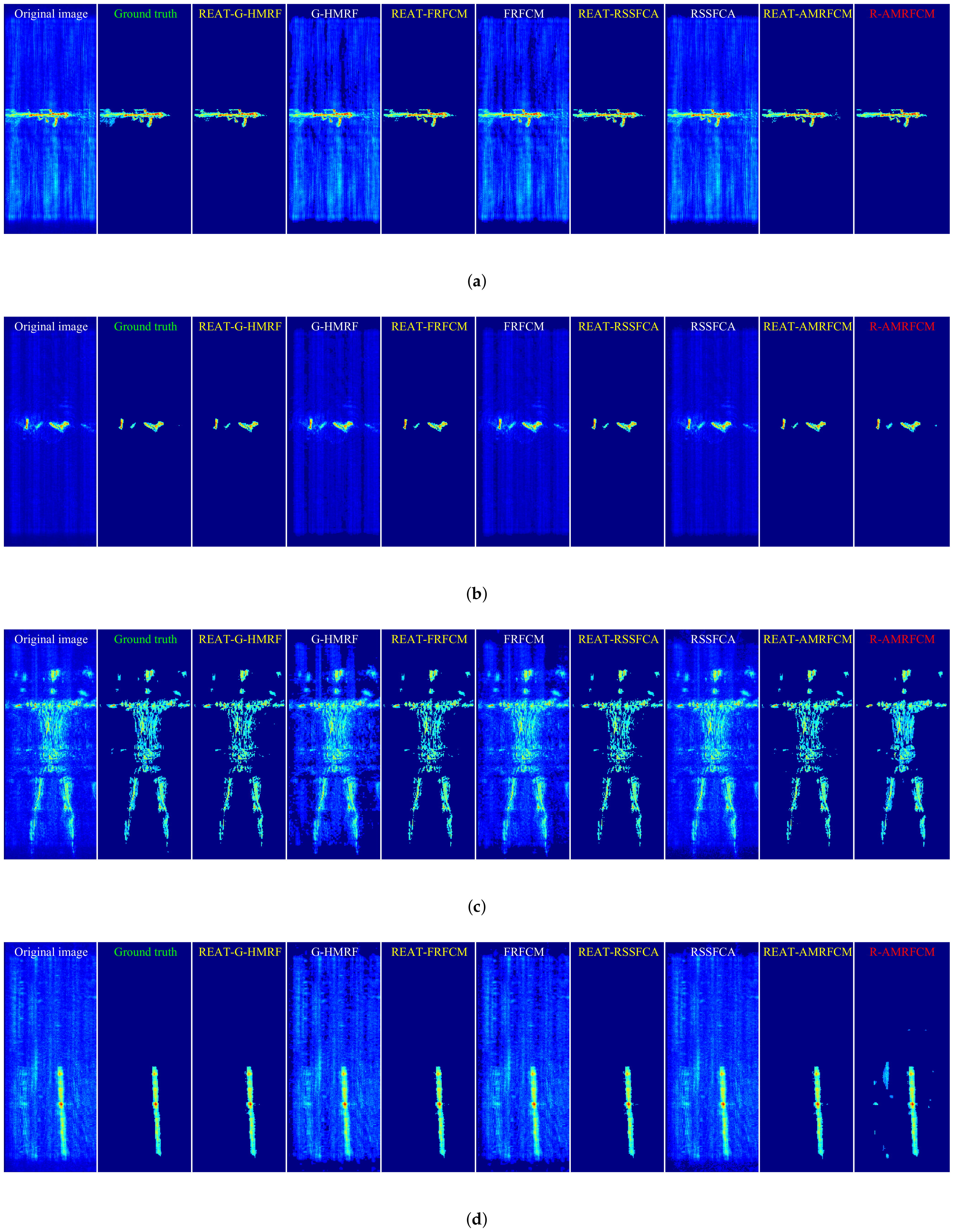
The target extraction results of the four images in the data set are shown in
Figure 5. For a clear display, we converted the 3-D image into a 2-D image with the maximum projection along the Z direction. The original image is in the leftmost column, and the ground truth is next to the original image. The results of the original algorithms are marked in white, the results of the algorithms enhanced by the REAT are marked in yellow, and the results of the state-of-the-art algorithms are marked in red.
As shown in
Figure 5, the target extraction results of the three original algorithms (G-HMRF, FRFCM, and RSSFCA) contain a lot of background voxels. In contrast, the extraction results of the three enhanced algorithms (REAT-G-HMRF, REAT-FRFCM, and REAT-RSSFCA) almost do not contain background voxels. Additionally, as shown in
Figure 5d, the result of REAT-AMRFCM contains fewer background voxels than that of R-AMRFCM. Therefore, the proposed algorithm enhances the anti-interference ability of the existing image segmentation methods and has a stronger anti-interference ability than the state-of-the-art algorithm.
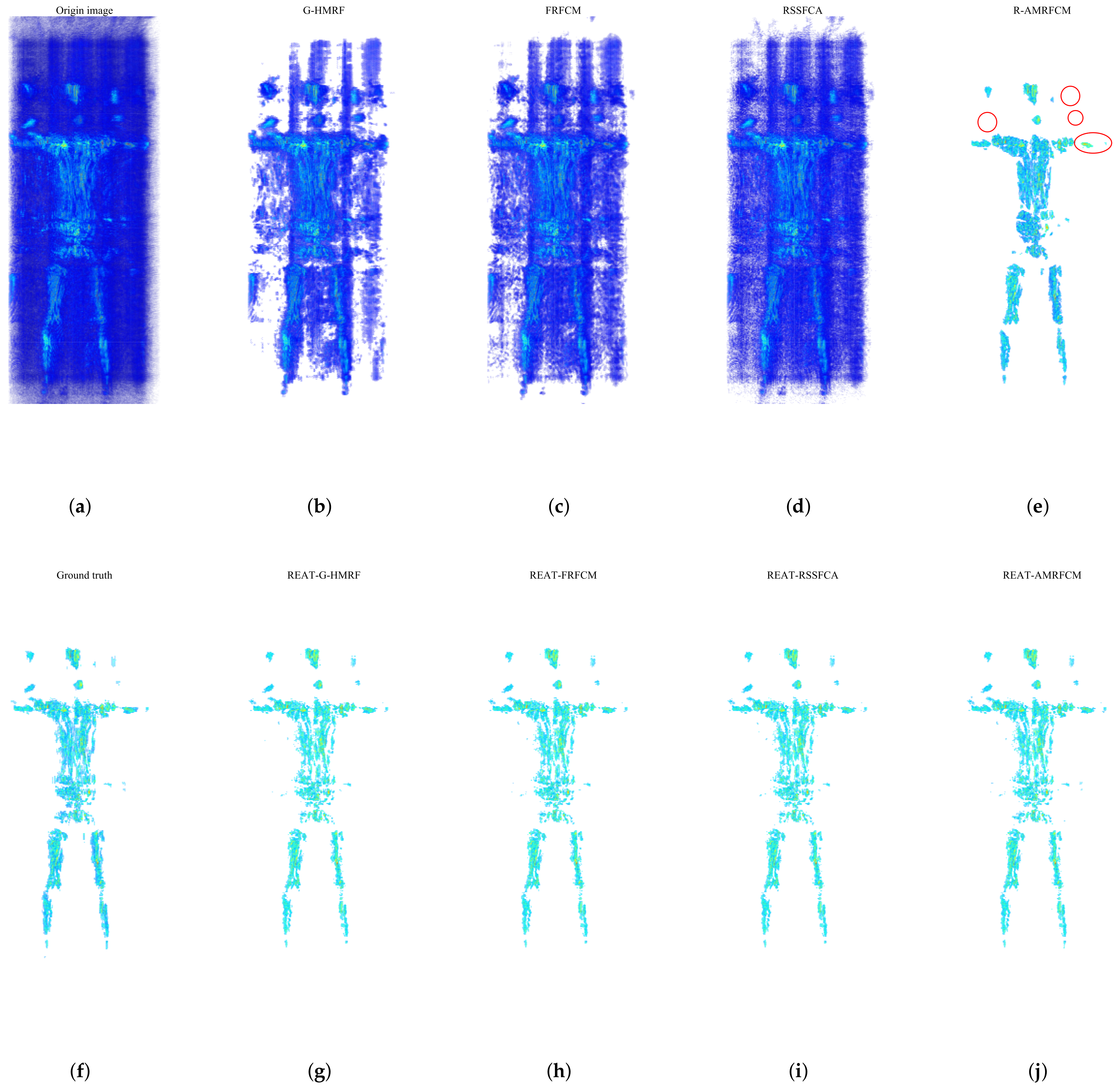
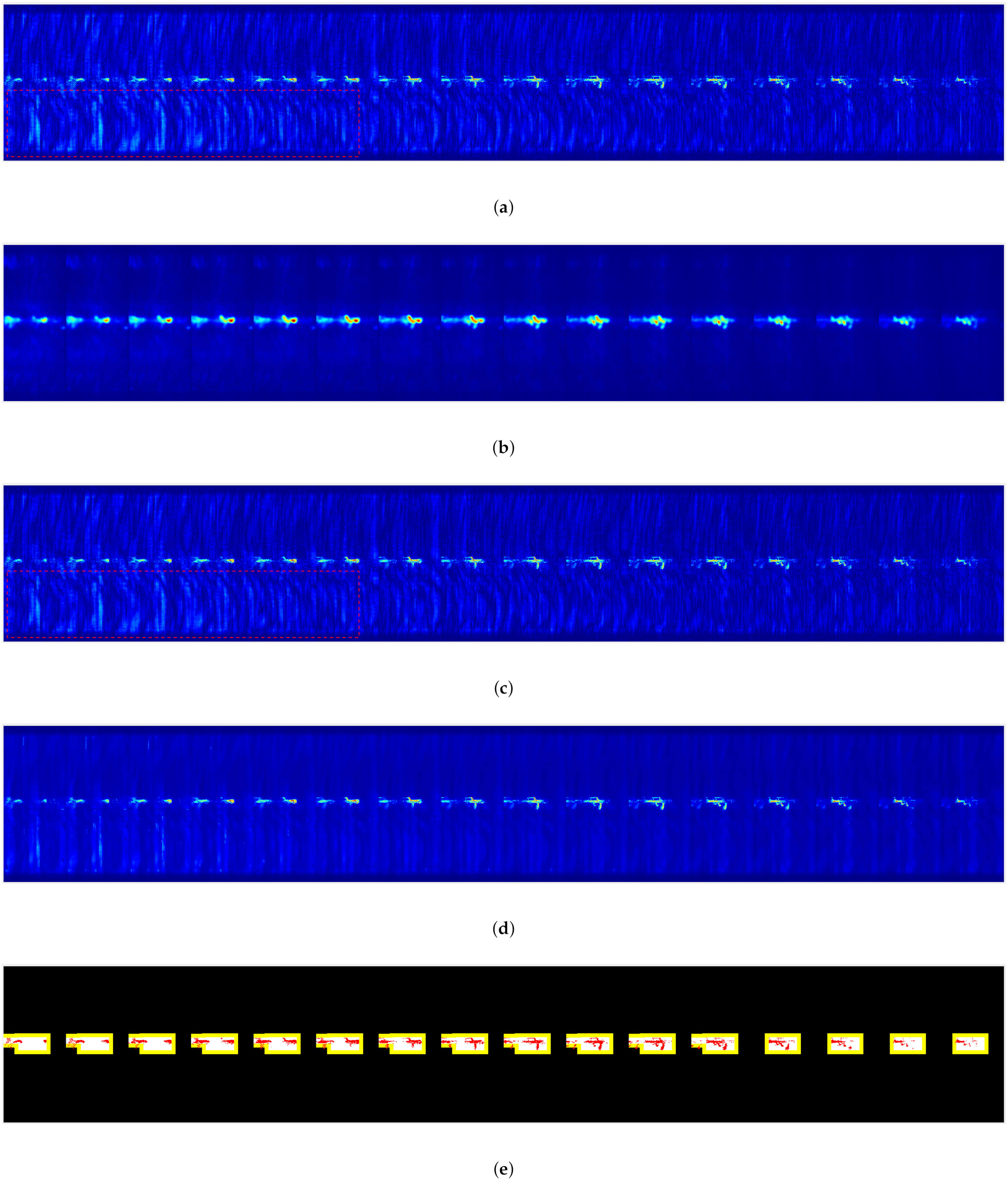
As shown in
Figure 6, there is a 3-D original image of the human body, a 3-D ground truth, and 3-D extraction results of 8 algorithms. The original image is shown in
Figure 6a. Visually, the side lobes and interference in the imaging space cover the main lobe.
Figure 6b–d are the extraction results of G-HMRF, FRFCM, and RSSFCA, respectively. The extraction results of these algorithms still contain a lot of background voxels (sidelobes and interference). As shown in
Figure 6e, R-AMRFCM effectively divides the target voxels and most of the background voxels. However, some regions in the extraction result are over-segmented, and a large number of target voxels are lost in some areas. The areas where the target voxels are lost are marked by red circles. As shown in
Figure 6g–j, the enhanced segmentation algorithms achieve excellent target extraction. There is no obvious over-segmentation and lack of target regions in these extraction results.
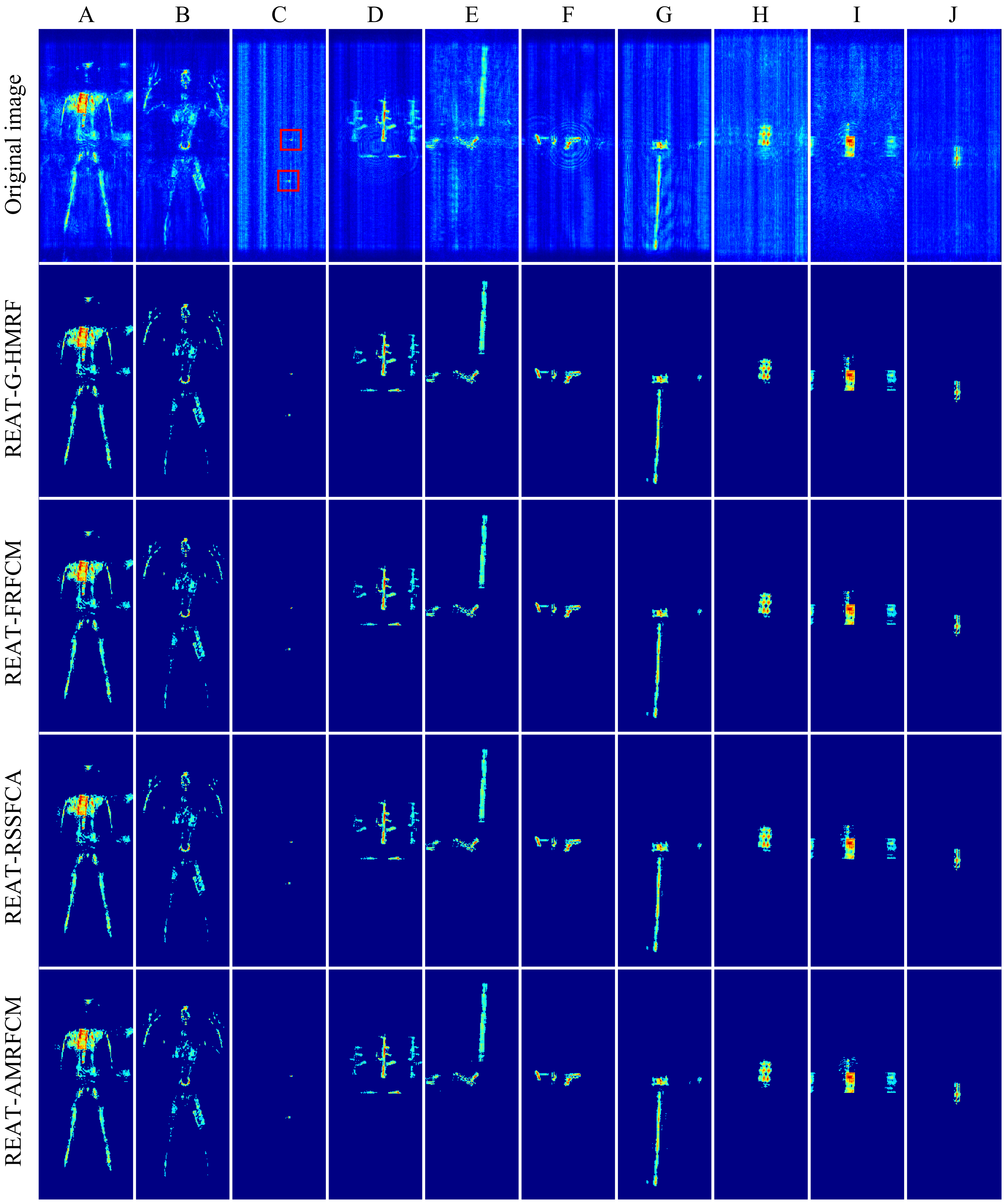
As shown in
Figure 7, the original SAR images and extraction results of 10 scenes are shown through the maximum projection. These scenes contain a rich variety of targets. For example, scene C contains two tiny objects: a tomato and a tiny metal ball. Although the extraction of tiny targets in a scene full of interference is a severe test for the algorithm, the algorithms enhanced by REAT still complete the target extraction. Scene D contains the main lobe and the grating lobes of a rifle and a knife. The grating lobes are regarded as the weak targets. Among these four enhanced algorithms, REAT-AMRFCM extracts more target grating lobes than the other three algorithms. Therefore, REAT-AMRFCM is better at classifying weaker voxels as target voxels than the other three enhanced algorithms.
5.3. Evaluation of the Performance
Accuracy, precision, recall, and the DSC are used to evaluate the performance of these algorithms. The evaluation results of the original algorithms and the enhanced algorithms are shown in
Table 1. The accuracy of these three enhanced algorithms is very close to 1. Additionally, their precision, recall, and DSC are all higher than 0.7989. Among them, REAT-FRFCM has the highest precision (0.9125), REAT-RSSFCA has the highest recall (0.8702), and REAT-G-HMRF has the highest DSC (0.8703). The accuracy, the precision, and the DSC of the enhanced algorithms are significantly higher than those of the original algorithms. The extraction results of the original methods not only contain almost all target voxels but also contain a large number of background voxels. The over-segmentation makes the original methods have a very high recall. In summary, the proposed algorithm effectively enhances the performance of the existing image segmentation methods.
The evaluation results of REAT-AMRFCM and R-AMRFCM are shown in
Table 2. The accuracy, precision, recall, and DSC of REAT-AMRFCM are 0.9994, 0.9170, 0.7920, and 0.8432, respectively. The accuracy, precision, recall, and DSC of R-AMRFCM are 0.9988, 0.7879, 0.8187, and 0.7792, respectively. Compared with R-AMRFCM, REAT-AMRFCM improves the accuracy, the precision, and the DSC by 0.006, 0.1291, and 0.0640. The recall of REAT-AMRFCM is only 0.0267 lower than that of R-AMRFCM. DSC is the most important criterion among the four criteria, and the DSC of REAT-AMRFCM is significantly higher than that of R-AMRFCM. Hence, the performance of REAT-AMRFCM is higher than that of R-AMRFCM.
Consequently, the image analysis and evaluation results show that the proposed algorithm effectively enhances the anti-interference ability of the existing image segmentation methods. Moreover, the proposed algorithm has better performance and anti-interference ability than the ROI extraction algorithm in the state of the art.
5.4. Analysis of Computational Efficiency
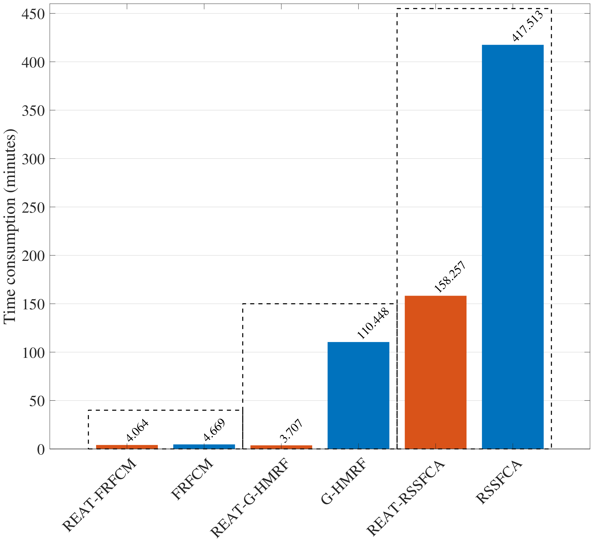
Computational efficiency is an important evaluation criterion. Therefore, we test the time consumption of the above-mentioned algorithms to process the entire data set. The time consumption of the original algorithms and the enhanced algorithms are shown in
Figure 8.
The orange bar represents the time consumption of the enhanced algorithms, and the blue bar represents the time consumption of the original algorithms. The time consumption of REAT-FRFCM is 12.96% lower than that of FRFCM. Although FRFCM has very high computational efficiency, the proposed algorithm still considerably improves the computational efficiency of FRFCM. The time consumption of REAT-G-HMRF is 96.64% lower than that of G-HMRF; thus, the proposed algorithm greatly improves the computational efficiency of G-HMRF. The time consumption of REAT-RSSFCA is 62.10% lower than that of RSSFCA, so the proposed algorithm also greatly improves the calculation efficiency of RSSFCA. Hence, the proposed algorithm causes a significant improvement in the calculation efficiency of the existing image segmentation methods.
As shown in
Table 3, the time consumption of REAT-AMRFCM and R-AMRFCM are 9.2528 min and 11.8387 min, respectively. The time consumption of REAT-AMRFCM is 21.84% lower than that of R-AMRFCM. Therefore, the proposed algorithm has higher computational efficiency than the ROI extraction algorithm in R-AMRFCM.
In summary, the proposed algorithm not only enhances the performance of the existing image segmentation methods, but also enhances their computational efficiency. Moreover, the performance and the computational efficiency of the proposed algorithm are higher than those of the state-of-the-art algorithm.


 ,
, 


