Article

Terrestrial Laser Scanning for Quantifying Timber Assortments from Standing Trees in a Mixed and Multi-Layered Mediterranean Forest

1
Dipartimento di Bioscienze e Territorio, Università degli Studi del Molise, Cda Fonte Lappone s.n.c., 86090 Pesche, Italy
2
Dipartimento di Agricoltura Ambiente e Alimenti, Università degli Studi del Molise, Via De Sanctis s.n.c., 86100 Campobasso, Italy
3
Department of Geodesy and Geoinformation, Technical University of Vienna, 1040 Vienna, Austria
4
Department of Innovation in Biological, Agro-Food and Forest Systems—DIBAF, University of Tuscia, 01100 Viterbo, Italy
*
Author to whom correspondence should be addressed.
Remote Sens. 2021, 13(21), 4265; https://doi.org/10.3390/rs13214265
Submission received: 31 August 2021 / Revised: 6 October 2021 / Accepted: 19 October 2021 / Published: 23 October 2021

Abstract

:
Timber assortments are some of the most important goods provided by forests worldwide. To quantify the amount and type of timber assortment is strongly important for socio-economic purposes, but also for accurate assessment of the carbon stored in the forest ecosystems, regardless of their main function. Terrestrial laser scanning (TLS) became a promising tool for timber assortment assessment compared to the traditional surveys, allowing reconstructing the tree architecture directly and rapidly. This study aims to introduce an approach for timber assortment assessment using TLS data in a mixed and multi-layered Mediterranean forest. It consists of five steps: (1) pre-processing, (2) timber-leaf discrimination, (3) stem detection, (4) stem reconstruction, and (5) timber assortment assessment. We assume that stem form drives the stem reconstruction, and therefore, it influences the timber assortment assessment. Results reveal that the timber-leaf discrimination accuracy is 0.98 through the Random Forests algorithm. The overall detection rate for all trees is 84.4%, and all trees with a diameter at breast height larger than 0.30 m are correctly identified. Results highlight that the main factors hindering stem reconstruction are the presence of defects outside the trunk, trees poorly covered by points, and the stem form. We expect that the proposed approach is a starting point for valorising the timber resources from unmanaged/managed forests, e.g., abandoned forests. Further studies to calibrate its performance under different forest stand conditions are furtherly required.

Graphical Abstract

1. Introduction

Roundwood represents one of the most important goods provided by forest ecosystems worldwide, feeding the forest products supply chain. Roundwood can be classified as industrial roundwood, such as raw logs (e.g., saw-log, pulpwood), and fuelwood for energy [1]. Despite the fact that roundwood production of Europe’s forests has been growing, reaching about 550 million m3 annually [1], recognizing the European countries as some of the main producers of industrial roundwood [2], uncertainties about timber assortment and fuelwood estimates are still unsolved. These uncertainties might be associated with the low performance of traditional surveys lacking for accurately depicting the trees’ architecture, since bark irregularities, such as bulges, holes, cavities, and other defects [3] are often ignored.
The tree characteristics such as stem tapering, stem curve, and stem diameter are among the most important tree variables required for assessing the timber assortments from standing trees [4,5]. Some studies proposed methods for extracting such tree characteristics, e.g., stem tapering, stem volume [6], and geometry wood defects (i.e., stem straightness) [7], from trees in coniferous and broadleaf forests. However, considering that most of the tree characteristics are based on cylinders’ models, as stem diameters [6], their accuracy is measured in function of the stem form and cross-sectional description. This means that such accuracy decreases, as the sweep deflection of stem and the occurrence of bark irregularities increase [3]. Measuring the tree characteristics on standing trees through traditional surveys became challenging, especially in deciduous or mixed forest stands [8]. Therefore, innovative and accurate methods aimed at assessing the timber assortments from standing trees could be useful for valorising the timber products from forests [9]. Moreover, its implementation can support the management of forests in light of Sustainable forest management (SFM) criteria and indicators [10].
Over the last decades, Terrestrial Laser Scanning (TLS) technology depicts immediately and accurately the tree architecture through georeferenced points [11]. The versatility of laser scanning data allowed scientists to use it to face several issues in distinct topics, such as forest biodiversity [12], forest ecology [13], forest productivity [14], and carbon stock [15], as well as for analysing the performance of models conditioned by both operational (design of sampling) and technical (i.e., aligning and assembling the scans) aspects, weather conditions and forest stand conditions [16].
Some studies highlighted that the assessment of the tree characteristics, such as stem diameter, using TLS data became easier to explore in forest plantations rather than in natural forests [11,16]. A powerful approach for deriving these tree characteristics from TLS data is named cylinder-fitting [16,17]. Practically, cylinder-fitting divides the TLS data into several horizontal slices, then it detects and measures the cylinders within each horizontal slice [18]. The stem position and stem curve for each stem are the main products of the cylinder-fitting approach. The validation of the cylinder-fitting is based on the curve length ratio (CLR) and the percent of the tree height covered (PHC) thresholds [16].
Despite several tools allow automatically extracting tree variables (i.e., tree height, stem volume) from standing trees using TLS data e.g., TreeQSM [19], Simple-Tree [20], Computree [14], and OPALS (Orientation and Processing of Airborne Laser Scanning data) developed by the Vienna University of Technology staff (Vienna, Austria) (Available from https://opals.geo.tuwien.ac.at; accessed on 15 August 2021), most of them fail with small trees, consider neither the timber-leaf discrimination nor pre-processing of TLS data, and are mainly focused on collecting forest inventory information from trees. However, OPALS became promising for scientists because it provides modules for the stem form reconstruction, such as a cylinder-fitting approach and pre-processing of TLS data [21], and machine learning became promising for the timber-leaf discrimination [13].
A feasible and robust procedure aimed at gathering timber assortment information of standing trees using the promising methods become highly needed to better use the timber resources, as well as to take timely and appropriate SFM-based decisions. However, despite the recent advances on timber productivity using TLS data, just a few studies used some of these for assessing the timber assortments from standing trees and even less focused on natural mixed forests [22,23]. This means that an approach including the promising approaches, such as cylinder-fitting and machine learning approaches can be effective for timber assortments assessment, even for supporting SFM. This study aims to introduce an innovative procedure using the promising approaches for assessing timber assortments from standing trees using TLS data in a natural mixed and multi-layered Mediterranean forest. This is the first study that accurately assesses different types of timber assortment from natural forests through a combination of timber-leaf discrimination and pre/post processing of TLS-data. This procedure is consisting of five steps: (a) pre-processing, (b) timber-leave discrimination, (c) stem detection, (d) stem reconstruction, and (e) timber assortment assessment. This approach could be a starting point for optimising the use of forest resources, reducing timber waste, valorising timber, and fostering carbon storage.

2. Materials and Methods
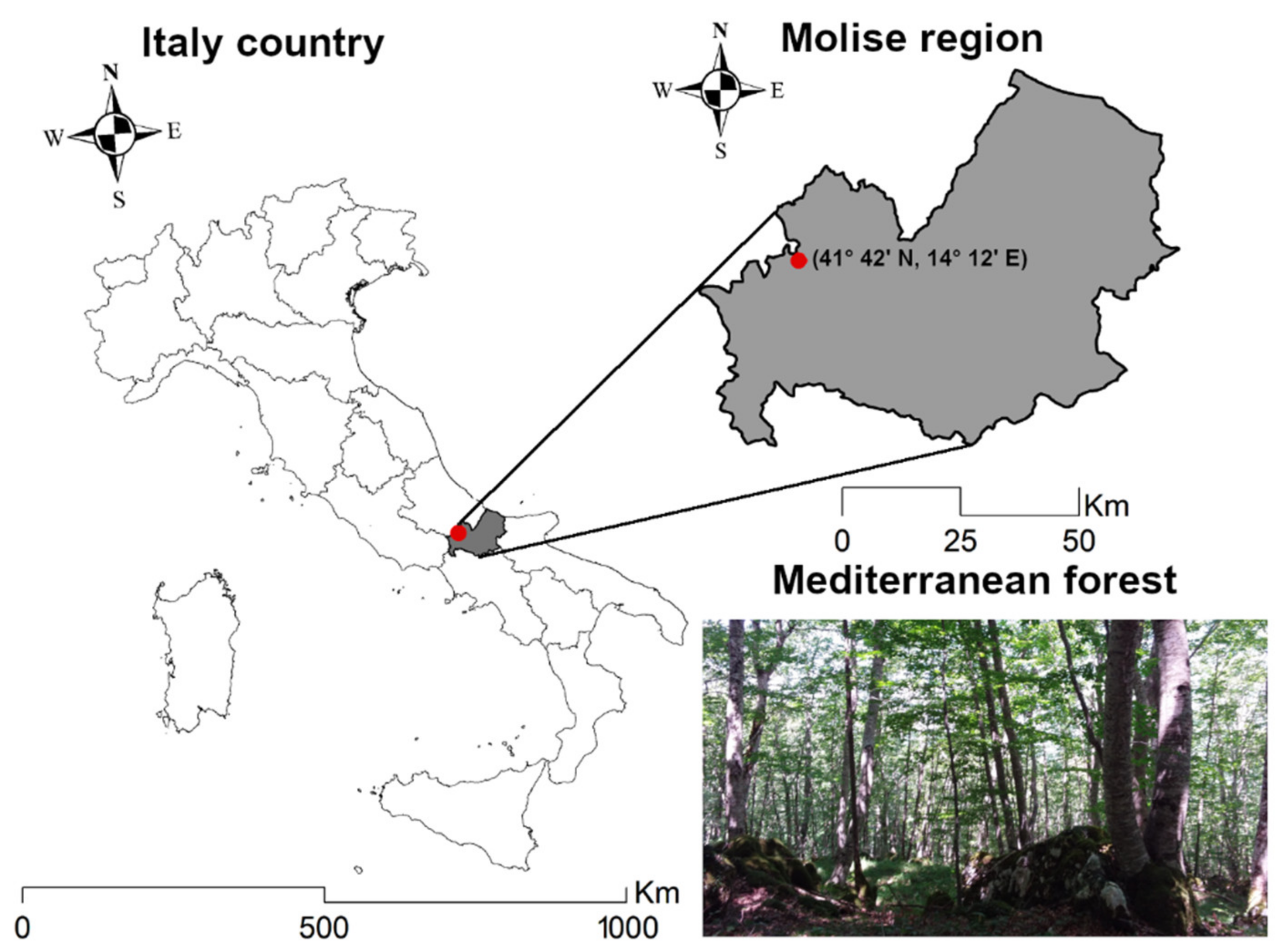
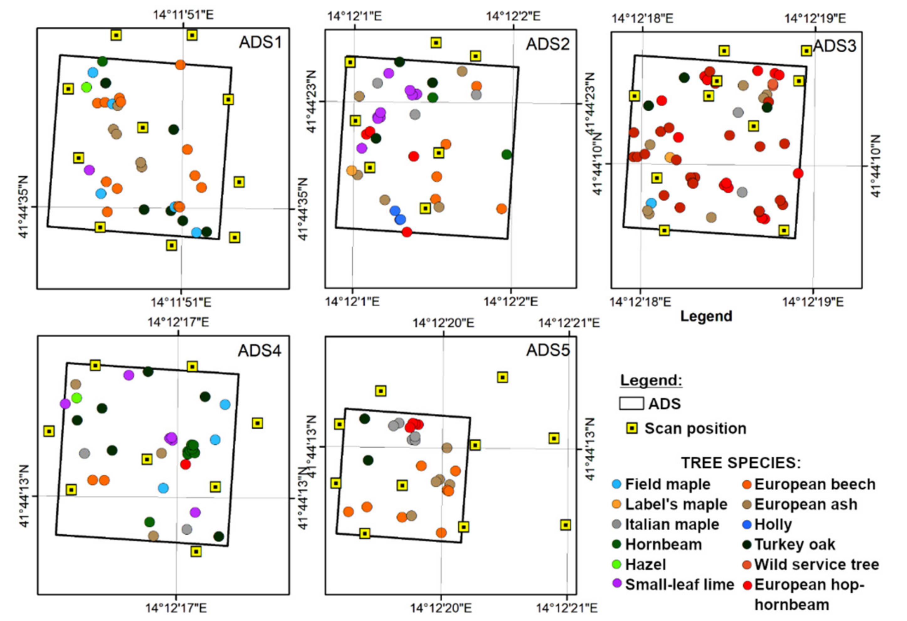
2.1. Study Area

The study area is located in the Molise region (Central of Italy, 41°42′N, 14°12′E), in a Mediterranean mixed forest called Bosco Pennataro (Figure 1). Bosco Pennataro is characterized by a high tree species richness including Turkey oak (40%), European beech (21%), Italian maple (9.6%) [24] and a heterogeneous forest structure. The forest of Bosco Pennataro is classified as oak–hornbeam forest type [25], belonging to the Natura 2000 network, moreover, it is recognized as a core area of the Man and Biosphere (MaB) reserve of Collemeluccio-Montedimezzo Alto Molise. Due to its ecological role, the forest was historically managed for productive purposes as an even-aged forest with natural regeneration, while in the last 50 years the harvesting activities were very limited and mainly focused on biodiversity conservation. As a result, currently, the forest is characterized by a high structural heterogeneity including tree microhabitat structures as indicators of biodiversity [26].

2.2. Field Data

The field survey was carried out in 2016 within five square plots (hereafter ADS) of 529 m2 (23 m × 23 m). All trees with a diameter at breast height (DBH) ≥ 0.025 m were measured through the Field-Map tool (https://www.fieldmap.cz/, accesssed on 31 August 2021). The surveyed tree variables were DBH, tree height (TH), stem position, canopy projection area (CPA), tree species, and tree vitality. Moreover, the stem volume (TSv) was calculated using specific allometric equations for Italian tree species in the National Forest Inventory [27].

2.3. Terrestrial Laser Scanning Data
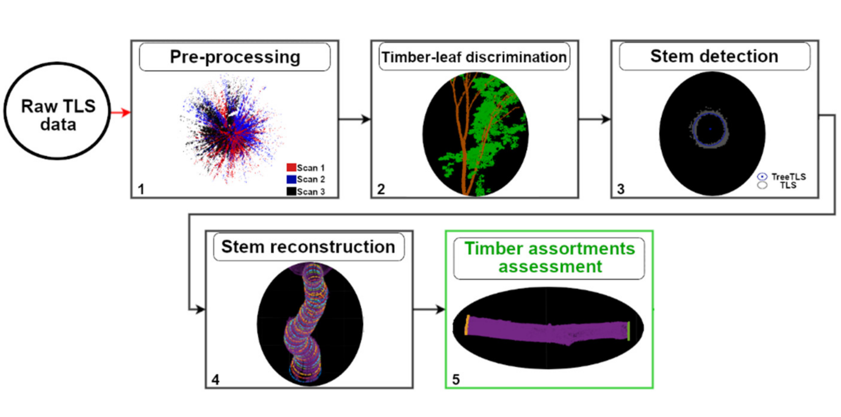
Terrestrial Laser Scanning (TLS) data was collected in July 2018 through Leica ScanStation (hereafter LSS) P30/40 device (https://leica-geosystems.com/it-it/, accesssed on 31 August 2021). LSS is a Laser 3D scanner suitable for collecting 1 million points per second for a wide range of up to 270 m. The laser scanning system used for this device was an Ultra-high-speed time-of-flight enhanced by Waveform Digitising technology. The horizontal and vertical field-of-view of the LSS was 360° and 290°, respectively. The distance measurement accuracy for objects was about ±2 mm. Several TLS scans (mean and ±SD = ~9 and ±1.4 scans) were taken in random positions within all five ADS, covering 178 single trees.

2.4. Data Analysis

The analysis of the TLS data consists of five steps: (1) pre-processing; (2) timber-leaf discrimination; (3) stem detection; (4) stem reconstruction and (5) timber assortment assessment (Figure 2).

2.4.1. Pre-Processing of the Raw TLS Data

As a pre-processing step, the collected raw TLS data was co-registered, aligned, and assembled using Leica Cyclone 360 3DR V.1.7.1000 software (https://leica-geosystems.com/, accesssed on 31 August 2021) and OPALS software version 2.4.0. e.g., opalsICP (https://opals.geo.tuwien.ac.at/html/stable/ModuleICP.html, accesssed on 31 August 2021). The co-registration was however supported by a list of recorded geographic coordinates taken in random positions through a GPS Trimble GeoXT mounted on a Hurrican Antenna. The obtained point registration accuracy was both lower than 0.25 of the plane roughness and 25° of the angle between the normal of corresponding points. The average distance between two adjacent points ranged between 3.19 mm and 5.22 mm among the five TLS data. To optimize tree crowns’ description and reducing the points for each ADS, we vertically clipped the point cloud provided by each ADS using a bigger box dimension equal to 729 m2 (27 × 27 m) than that used for field surveys (529 m2; 23 × 23 m). The full processing was performed using a batch script including several OPALS modules, such as opalsImport, OpalsICP, opalsAlgebra, and opalsExport (https://opals.geo.tuwien.ac.at/, accesssed on 31 August 2021). The final files (LAS Format) produced by the pre-processing consisted of geographic coordinates (i.e., x, y, z) and intensity features; these were used as input data in the subsequent steps.
After the pre-processing, additional tree variables other than those surveyed during the inventory campaign were manually measured in each point cloud from the TLS data using the point picking tool embedded in CloudCompare software. Such variables allowed us to describe the stems based on log measurements. The tree variables were taken in all trees with a DBH ≥ 0.20 m [7,16,28] Their measurements were taken in the trunk section ranging between the tree height at 0.50 m (hereafter THbase) and the tree height at the first attached branch (TH1). The tree variables were maximum-end diameter (Dmax), minimum-end diameter (Dmin), and length of log (L). We calculated the log volume (hereafter TTv.log) using these variables through the Smalian formula (Equation (1)).
TTv.log = (Dmin2 + Dmax2)/8 × π × L
where: TTv.log is the log volume, (m3); Dmax is the maximum-end diameter of the log, (m); Dmin is the minimum-end diameter of the log, (m); L is the length of the log, (m); and π –3.1416.
In addition, the logs manually measured through CloudCompare software were classified into merchantable (2.5 m ≤ x ≤ 3 m; length of the log) and non-merchantable (2.5 m < x; length of the log) types [29] (Figure 3). Based on this assumption, trunk volume (hereafter TTv. Trunk) was calculated by summing the TTv.log for both log types. After the classification of logs, two tree characteristics e.g., straightness (STR; cm m−1; Equation (2)) and tapering (TAP; cm m−1; Equation (3)), were extracted for the merchantable logs. This is because the STR reports how the stem axis is straight/sweep and TAP reports the changes of cylinders’ diameter along the length of the stem (Table 1) [7]. Both are useful information for validating the timber quality of stems. For both two equations, Dmin and Dmax variables were scaled from m to cm.
STR = h/L
TAP = (Dmax − Dmin)/L
where: STR represents the straightness of the log, (cm m−1); TAP represents the tapering of the log, (cm m−1); L is the length of the log, (m); Dmax is the maximum-end diameter of the log, (cm); Dmin is the minimum-end diameter of the log, (cm); and h represents the perpendicular distance (90°) between the highest convex curve and the straight line between Dmin and Dmax (Figure 3).
Based on the STR, and Dmin, merchantable logs were classified into 15 timber assortment quality classes, belonging to five timber assortment types, described by [7].

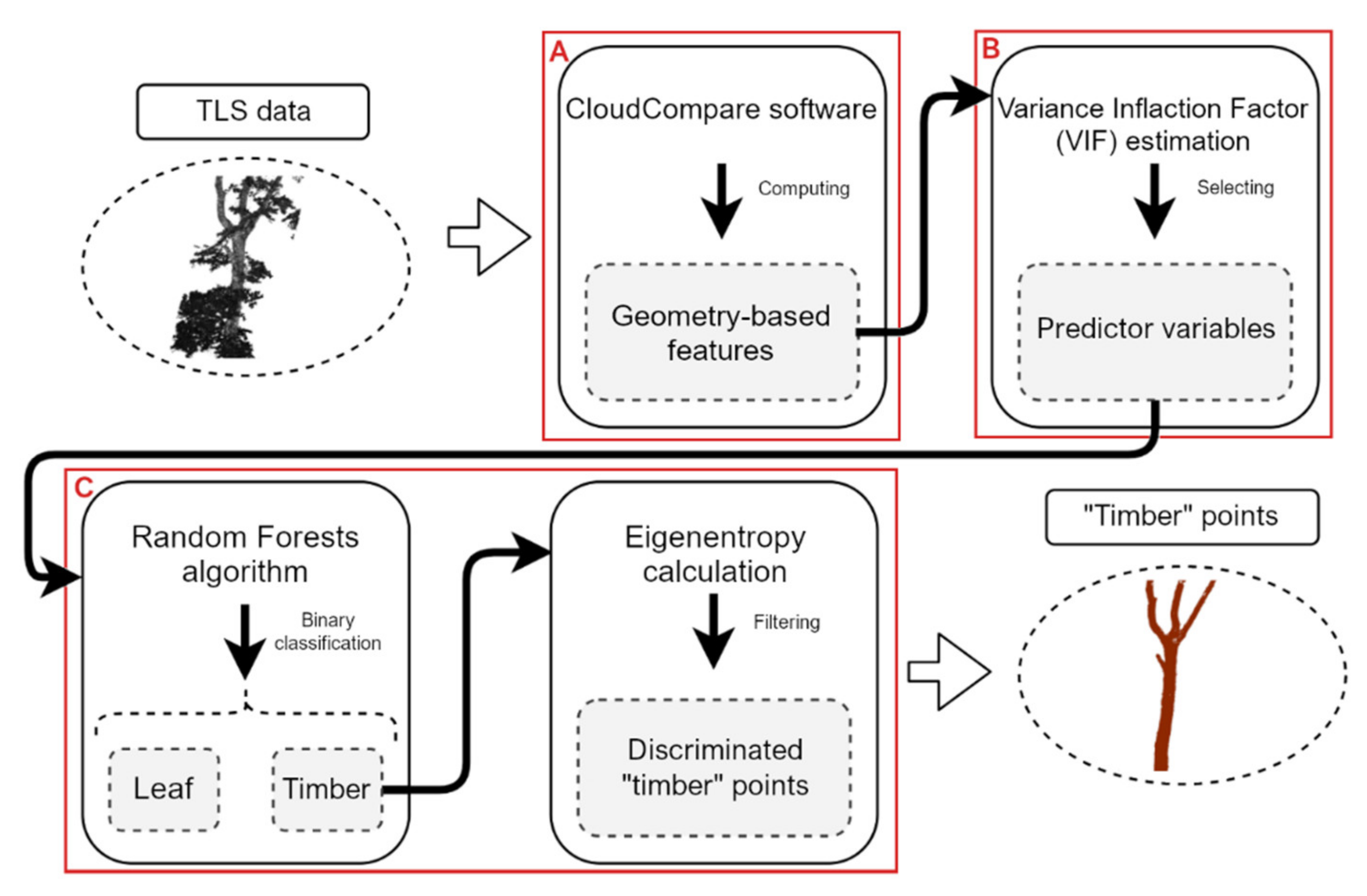
2.4.2. Timber-Leaf Discrimination

To discriminate timber from leaf points, we followed a step-by-step approach consisting of three sub-steps: (a) geometry-based calculation, (b) predictor variables selection and (c) binary classification (Figure 4).

Geometry-Based Calculation

Eighteen geometry-based features (i.e., roughness, mean curvature, Gaussian curvature, Gaussian normal change rate, number of neighbours, surface density, volume density, the sum of eigenvalues, omnivariance, eigenentropy, anisotropy, planarity, linearity, first and second principal component analysis, surface variation, sphericity, and verticality) were generated according to local neighbourhood radius approach (hereafter Ln). The optimal “Ln” was set to 0.07 m [30]. The processing was automatically performed using the “compute geometric features” tool embedded in CloudCompare v. 2.11.1 open-source software (http://www.danielgm.net/cc/, accesssed on 31 August 2021) [31] (see Appendix A). The eighteen geometry-based features joined to their geographic coordinates (.txt Format) were used as input data in the subsequent sub-step.

Predictor Variables Selection

We implemented the variance inflation factor (VIF), using 5 as a score threshold [32], for selecting the most explicative geometry-based features (hereafter predictors). The VIF score allowed us to ponder the correlation, collinearity, and multicollinearity among predictors, assessing their role in the precision of the binary classification model. To estimate the VIF score of the predictors, we used the “vifstep” function available in “usdm” R package [33]. The final product consisting of a list of eight predictors (i.e., anisotropy, the sum of eigenvalues, Gaussian curvature, mean curvature, PCA2, roughness, verticality, volume density) joined to their geographic coordinates (.txt Format) were used as input data in the subsequent sub-step.

Binary Classification

To classify the points from TLS data as timber and leaf labels, we followed a binary classification through Random Forest (RF) algorithm. RF algorithm is suitable to build multiple decision trees from randomly input training data for classification analysis [34]. We chose RF because it was faster, easier, and more accurate than other machine learning algorithms [13]. Before computing the RF, we prepared the training and testing input data of a representative proportion of point cloud data for each ADS. In this respect, we manually extracted the 10% of the point cloud for each ADS; then, we classified the points as timber and leaf labels; subsequently, we used their predictor variables as input data for classifying the remaining points of each TLS data. Thereafter, we computed the RF algorithm through Weighted Subspace Random Forest for Classification (wsrf) R package, [35]. As regards the “wsrf” customizing, the “Ntree” was set to 2500, the “Mtry” was set to 3–4, and the “node size” was set to 5.
To efficiently discriminate the leaf from timber points, we removed the noise points found in the points classified as “timber”. To reach this, first, we recalculated the eigenentropy feature following the same previous procedure (Geometry-based calculation) [36]. Then, extreme eigenentropy values (0.03 ≤ x ≤ 0.75 ≡ 3th ≤ x ≤ 75th percentile; eigenentropy values ranging between 0 and 1) were removed of “timber” points [31]. The binary classification was validated through three statistic measurements: sensitivity, specificity, and accuracy measurements [13]. The sensitivity represents the percentage of points correctly identified (true positive), the specificity represents the percentage of points correctly excluded (true negative) and the accuracy represents the proportion of true positive values. The validation approach was computed using the “pROC” R package [37]. The “timber” points (.LAS Format) were used as input data in the subsequent step.

2.4.3. Stem Detection

This step aims to find the potential stem position and to measure the DBH of eventually detected trees from “timber” points through a raster-based approach embedded in OPALS modular program. OPALS, especially the opalsForest module (https://opals.geo.tuwien.ac.at/html/stable/pkg_opalsForest.html, accesssed on 31 August 2021), is a suitable tool for modelling the stems.
Before detecting the stem position, the topographic models Digital Terrain Model (DTM; 0.05 m) and Digital Surface Model (DSM; 0.20 m), were generated for each ADS using opalsDSM and opalsGrid modules. The normalization of the TLS data, using both the DTM and the DSM, was done with the opalsAddinfo module. The stem detection was based on TLS data of a horizontal slice between 1 m and 2 m above the ground. Using a voxel-based analysis, stem positions were detected based on different statistical information (i.e., sum, mean and maximum) related to voxel columns within the investigated horizontal slice. The voxel size was set to 0.01 m3. Since the trade-off between filled and gap voxels simulate many cylinders on the horizontal slices, the detection of trees was performed using such information through a seed region growing algorithm (python script is available at https://opals.geo.tuwien.ac.at/html/stable/ModuleDBH.html, accesssed on 31 August 2021).
The stem detection was validated through true-positive (TruePos; units) representing the correctly identified trees; false-positive (FalsePos; units) representing the commission error; false-negative (FalseNeg; units) representing the omission error, the detection rate and completeness (DR and completeness; %) representing the relationship between TruePos and observed trees and the correctness (correctness; %) representing the relationship between TruePos and number of stems extracted from TLS point cloud (TreeTLS).
The DBH cylinders were performed using the detected trees through the least-squared cylinder-fitting approach implemented in opalsDBH. The validation of the DBH was performed through two linear regression models. The first model used all observations, and the second used all observations without potential outliers. The potential outliers were calculated using the Cook’s distance, considering as potential outliers those observations overcoming a Cook’s distance of 3 times greater than the average distance values [38]. DBH regression models were built using “stats” (authors, R Core Team, and contributors worldwide) and “car” R packages [39].

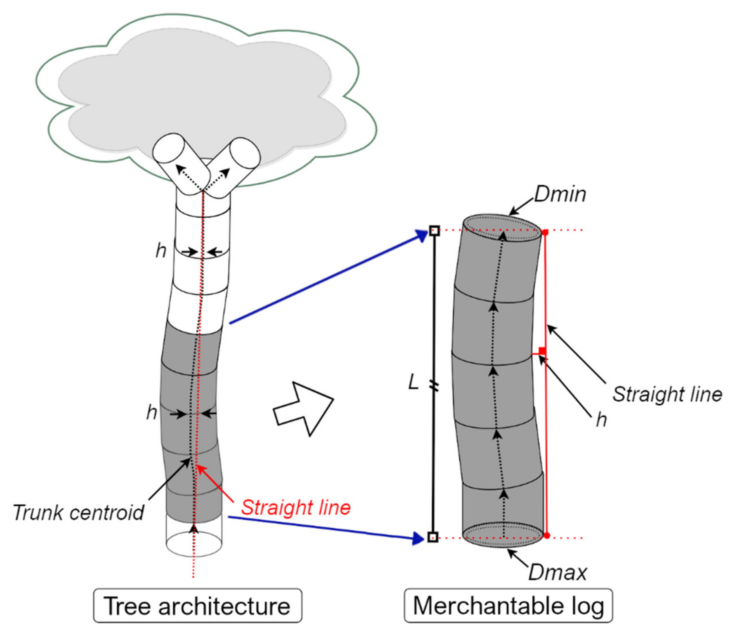
2.4.4. Stem Reconstruction

For reconstructing the trees, we tracing the measured cylinders along the stem x-axis through the cylinder-fitting approach embedded in opalsDBH. OpalsDBH is a suitable module to detect, measure and trace the cylinders along the trunk, allowing the stem curve description [16]. Although the tracing of cylinders from OpalsDBH begins from the bottom to the top along the stem, to ensure consistency, the DBH measurement was used as an anchor point for accepting or rejecting the predicted cylinders’ measures. This leads us to reconstruct the stem accurately. However, to run opalsDBH, some mandatory parameters, such as trace, overlap, and patchLength, were required: “trace” representing the option enabling the tracing of cylinders, “overlap” representing the percentage of overlap patches between two traced cylinders, and “patchLength” representing the length of a shift vector between two consecutive patches. In this study, the “trace” was set to 1–1, the “patchLength” was set to 0.5 and the “overlap” was set to 0.8.
The validation of the stem reconstruction was performed using four different parameters: reconstructed stem from TLS data (RStem; units) representing the number of reconstructed stems; RStem rates (TrueRStem; %) representing the relationship between RStem and observed trees; curve length ratio (CLR, %) representing the relationship between the proportion of the stem length covered by the extracted stem curve from TLS data and that obtained from observed data [16]; percent of the tree height covered (PHC, %) representing the relationship between the proportion of the stem length covered by the extracted stem curve from TLS point cloud and the tree height from observed data [16]. Since the PHC is strongly conditioned by the length of the TH1, we did not compare this result with that obtained in other studies. We used the “stats” (authors, R Core Team and contributors worldwide) and “usdm” [33] R packages in this processing. The stem curve data (.shp and .txt Format) for each ADS was used as input in the subsequent step.

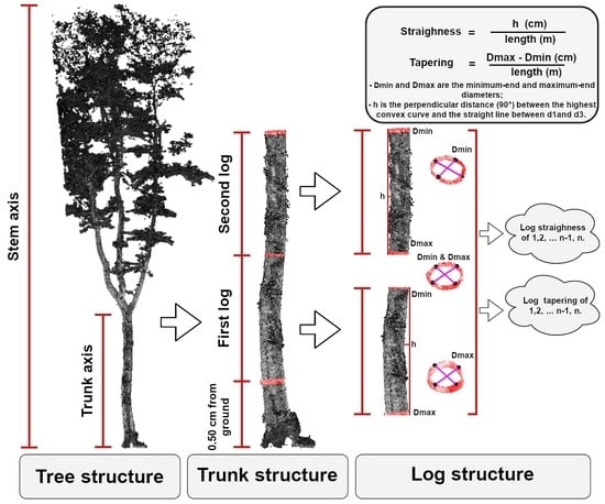
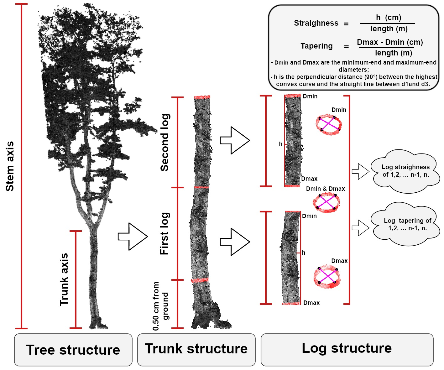
2.4.5. Timber Assortment Assessment

For extracting the timber assortment information from TLS data, first, we quantified the logs, then we characterized the merchantable logs, and then we classified the merchantable logs.
The log quantification, which was based on the stem curve data, was performed using R software. The extracted stem curve data for each tree, corresponding to infinite cylinders, was divided into two group types of cylinders. The large group corresponds to merchantable log (2.5 m < x < 3 m; length of the log) and the small group corresponds to non-merchantable log (2.5 m < x; length of the log). To better simulate the strategy for measuring the STR and TAP indicated by [7], we used three cylinders’ data for each merchantable log (“first cylinder”, “second cylinder” and “third cylinder” representing Dmax, central, and Dmin). Here, we used the mean, standard deviation (±SD) to validate the accuracy of the log quantification. The validation of the TTv.log was performed using two linear regression models including and excluding potential outliers based on Cook’s distance.
The log characterization, which was based on the equation for deriving the STR and TAP, was adjusted and implemented in one mathematical R function [7]. The result was validated by comparing predicted vs. observed STR and TAP values, specifically, the mean and the standard deviation (±SD), the bias and the root mean squared error (RMSE) were used for the validation.
The merchantable log classification, which was based on the timber quality (i.e., STR and Dmin), was performed using a R function in R software version 3.6.2. Particularly, such a R function uses the thresholds indicated in Table 1 for assigning one timber assortment class to each merchantable log. The validation was done by comparing the predicted vs. observed number of merchantable logs by type. Furthermore, the bias was used for the validation. Overall, the R packages used for timber assortment assessment were “stats” (authors, R Core Team, and contributors worldwide), “dplyr” [40] and “usdm” [33]. However, the regression models required the “stats” (authors, R Core Team, and contributors worldwide) and “car” R packages [39].

3. Results

Results reveal that all five ADS have a huge tree species richness and structural heterogeneity (Table 2). The abundance of tree species richness ranged between 5 and 9 tree species; the most frequent tree species are European beech (28.7%), European ash (14%), European hop-hornbeam (12.4%), and Turkey oak (11.8%) (Figure 5). However, observed trees, belonging to twelve tree species, results in displaying by point clouds (Figure 6).
Among the ADS, the different forest structure is supported by the DBH, ranging between 0.16 m and 0.26 m, the TH, ranging between 13.28 m and 23.10 m, and the TSv, ranging between 13.20 m3 and 25.29 m3 (Table 2). In contrast to these measurements, the stem density can be divided into three difficulty levels among the ADS: low (<500 trees ha−1), moderate (500–900 trees ha−1), and high (>900 trees ha−1). The structural heterogeneity among ADS is even impacted on the point density and spacing of TLS data varying between 36,622 pts m−2 and 5.22 mm and 92,244 pts m−2 and 3.29 mm. About TLS data, the number of randomly distributed scans around the center ranging between 7 and 10 among the ADS allowed us to describe the vertical and horizontal profiles of trees (Figure 5).
Results show that more than one-third of the observed trees, corresponding to 70 out of 178 observed trees, are suitable for timber assortment assessment, as the DBH is larger than 0.20 m. Such large trees are consisting of European beech (32.9%; 23 trees), Turkey oak (21.4%; 15 trees), European ash (14.3%; 10 trees) and Italian maple (11.4%; 8 trees), and other four broadleaved species (20%; 14 trees). These large trees store 306 merchantable and 79 non-merchantable logs (Table 3). Most of the merchantable logs are either slightly or strongly contorted based on variable STR values, ranging between 1.4 cm m−1 and 2.9 cm m−1, and TAP, ranging between 1.1 cm m−1 and 1.8 cm m−1, measurements. The merchantable logs accumulate 10 times more volume than non-merchantable logs.

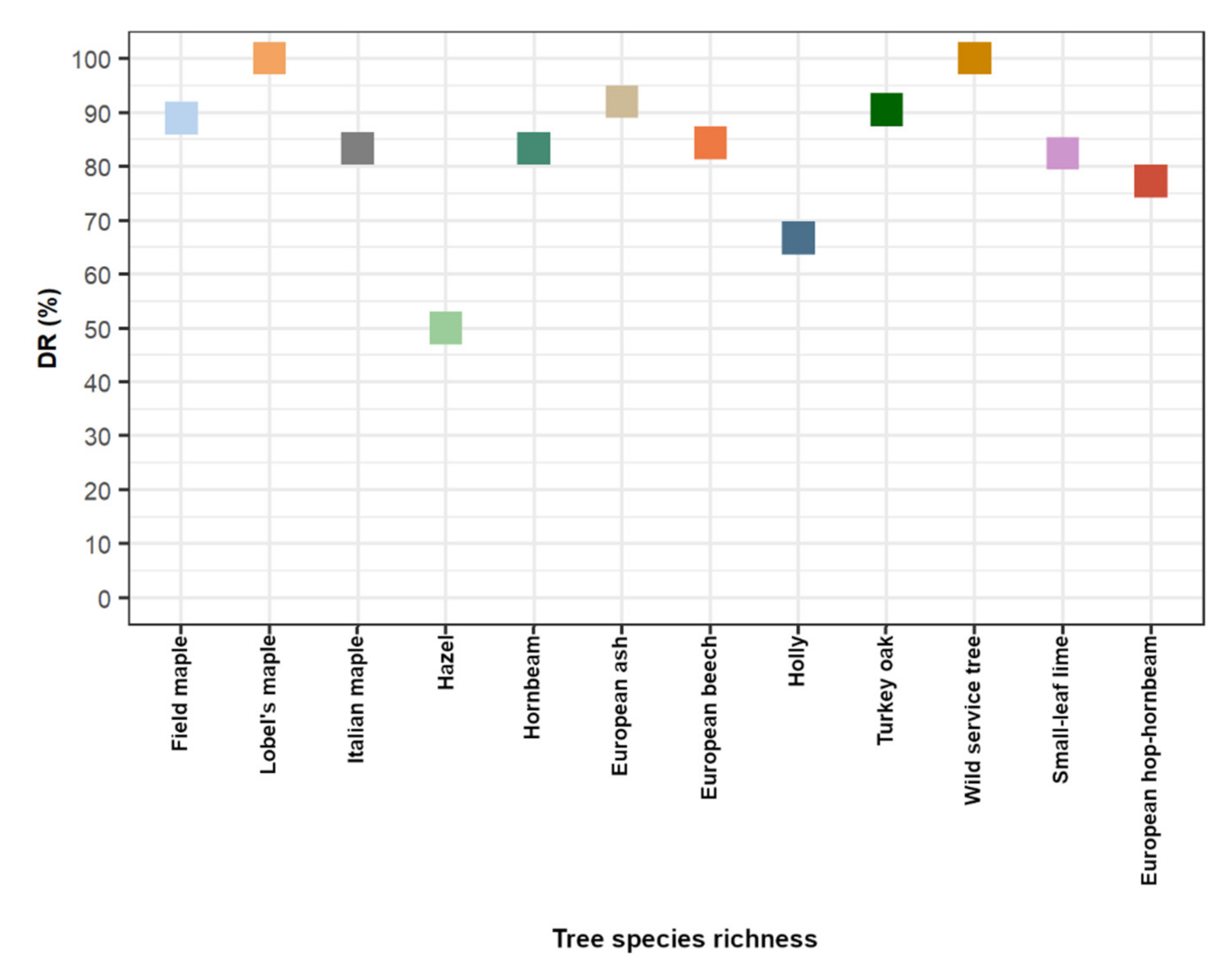
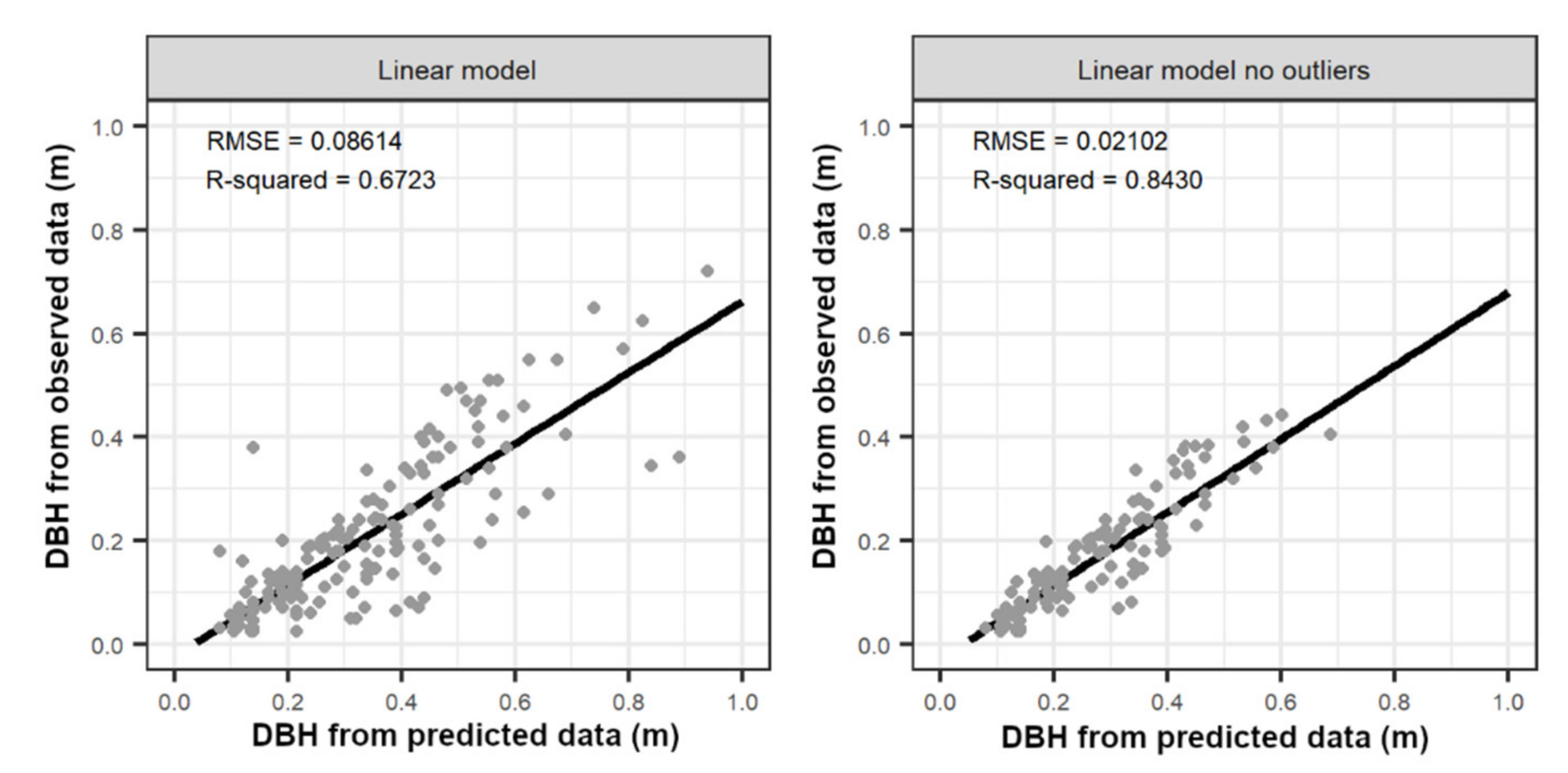
3.1. Timber-Leaf Discrimination, Stem Detection, and DBH Estimation

Results show that the RF algorithm provided accurate timber-leaf discrimination in a mixed and multi-layered forest. For all five ADS the accuracy is 0.98, the sensitivity is 0.98 and the specificity is 0.98.
We detected 151 out of 178 observed trees, reaching an average detection rate accuracy equal to 84.4%, with a high uniformity/similarity among the ADS (standard deviation, ±SD = ±4.7%; Table 4). The results reveal that the stem detection approach is more sensitive to the commission error (84 as the sum of FalsePos) than the omission error (27 as the sum of FalseNeg), which is also supported by different patterns of completeness (84.4%) and correctness (66.9%) accuracies (Table 4). All trees with a DBH higher than 0.30 m are correctly detected.
Results reveal that stem detection is more affected by point density than stem density. Particularly, the detection of trees is more accurate in ADS with a high point density (≥44,210 pts m2; corresponding to moderate/high stem density levels) than those with a low point density (36,622 pts m2; corresponding to low stem density levels) (Table 2 and Table 4). Hence, the detection rate ‘DR’ increases as point density increases. We found the lowest DR in the forest with a low stem density (<500 trees ha1) accordingly. Particularly, we detected 45 out of 52 observed trees of the ADS belonging to the high stem density; we detected 87 (sum of true positive for ADS 1, 2, and 4) out of 102 (sum of trees observed for ADS 1, 2, and 4) observed trees of the ADS belonging to the moderate stem density; we detected 19 out of 24 observed trees of the ADS belonging to the low stem density.
Results reveal that stem detection is even affected by tree species richness. Particularly, the detection of trees is more accurate in ADS with high (ranged from 7 to 9 tree species) than low (5 tree species) tree species (Table 4). Comparing the ADS with a similar number of tree species (ADS 2 and 4; 9 tree species), we observed better DR accuracy in the ADS with low (ADS 4 = 33 trees) than high stem density values (ADS 2 = 36 trees). Nevertheless, among the 12 tree species, we found a better DR accuracy for Lobel’s maple, Wild service tree, European ash, Turkey oak, Field maple and European beech (DR > 84.3%) (Figure 7).
The DBH detection is better (R-squared = 0.84; RMSE = 0.02 m) using all observations without potential outliers, than those with outliers (R-squared = 0.67; RMSE = 0.08 m) (Figure 8). The non-circular shape of the trunks, bark irregularities and the stem axis profile negatively affect the DBH predictions, based on Cook’s distance (greater 3 times). In total, Cook’s distance selects about 27 observations (∼15%) as outliers, these mainly are overestimated values that come either from large or small stems.

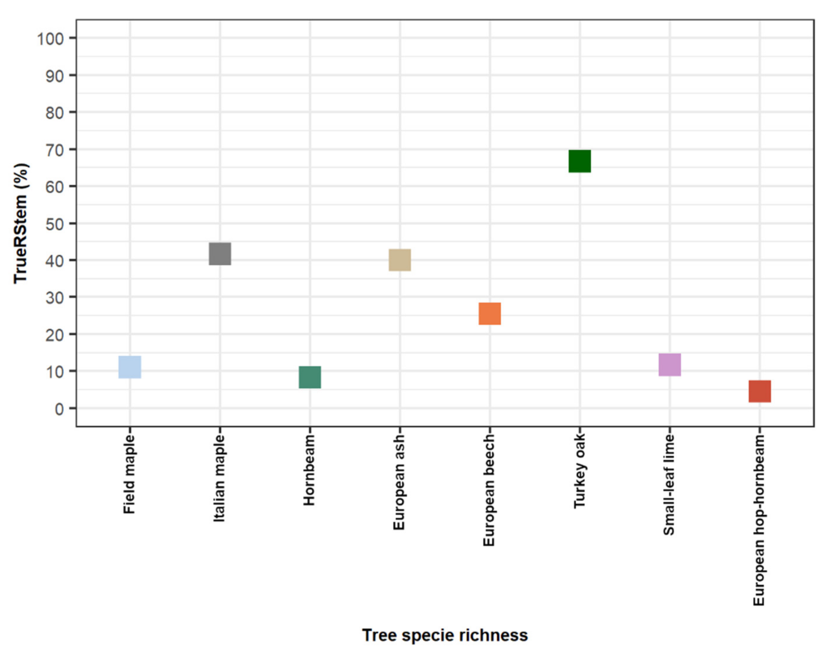
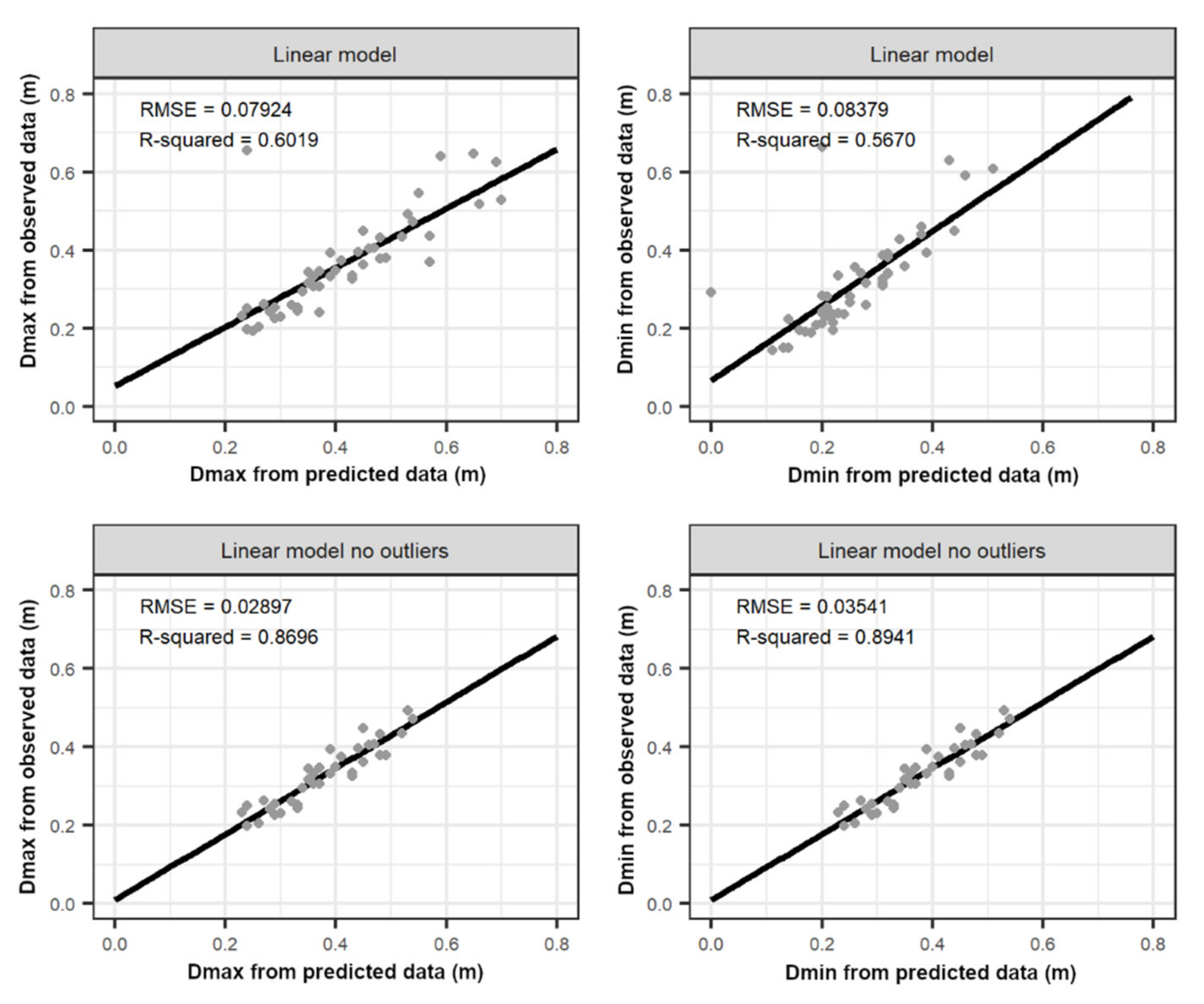
3.2. Stem Reconstruction

We reconstructed 47 out of 70 observed trees reaching an average stem reconstruction accuracy equal to 67.2%, with a low similarity/uniformity among the ADS (standard deviation, ±SD = ±14.86%) (Table 5). The role of the point density in stem reconstruction is less marked than that observed on stem detection (Table 5). Particularly, the stem reconstruction accuracy of the ADS with highest (ADS 1; 92244 pts m−2) and lowest (ADS 5; 36622 pts m−2) point density is rather similar (~70% of TrueRStem). The stem reconstruction is better in ADS with low/moderate than high stem density (Table 5). Nevertheless, the stem reconstruction becomes more accurate for Turkey oak, Italian maple, and European ash tree species (see Appendix B, Figure A1).
Results show that a large part of the trunk sections between THbase and TH1 is covered by cylinders, based on high values of CLR (mean = 88.1%; ±SD = ±16.7%; Figure 9A). This outcome, however, highlighted that the section covered by the cylinder is small compared to the total trunk section, based on the low values of PHC (mean = 35.4%; ±SD = ±11.3%) (Figure 9B). However, about 80% of trunks (39 out of 47 reconstructed trees) are correctly reconstructed (Figure 9A) until the TH1. Conversely, the PHC values show that about 75% of trunks are partially described by cylinders (30% < PHC < 68.3%), and the remaining ones are poorly described by cylinders (PHC < 29.9%; Figure 9B).

3.3. Timber Assortment Assessment

A total of 179 merchantable logs and 40 non-merchantable logs are available from 47 reconstructed trees. About 75% (134 out of 179 merchantable logs and 34 out 40 non-merchantable logs) of logs are correctly quantified (Table 6). On the one hand, comparing the predicted with the observed length of logs, more fitted predictions are found in merchantable (2.50 m vs. 2.78 m) with respect to non-merchantable logs (1.35 m vs. 1.62 m) (Table 6). On the other hand, our approach proved to be suitable to predict more than 70% of the total merchantable logs for all reconstructed tree species (see Appendix C, Table A1).
As concern the assessment of TTv.log, better accuracy is obtained excluding potential outliers (R-squared = 0.92; RMSE = 0.03 m3) from the regression compared to the inclusion of outliers (R-squared = 0.77; RMSE = 0.06 m3) (Figure 10). Slight overestimation of Dmin and Dmax negatively affects the TTv.log calculation, therefore, the performance of the model improves excluding potential outliers based on Cook’s distance (see Appendix D, Figure A2). In total, Cook’s distance selects 12 (∼8%) observations as outliers, these mainly belong to big logs (>0.33 m3).
Log characterization: most merchantable logs are contorted, based on STR patterns (mean 1.68 cm m−1; ±SD = ±1.73 cm m−1). The characterization of logs proved to be more accurate for STR than TAP measurements as confirmed by the different bias and RMSE values (Figure 11) found for TAP (1.69 cm m−1; RMSE 2.49 cm m−1) and STR (0.77 cm m−1; RMSE 1.88 cm m−1). Despite the validation of TAP showing a slightly low accuracy, we observed a similar trend between predicted and observed data.
Eleven out of 14 assortment types are accurately classified based on their estimated low bias (−1.36 number of logs by assortment class) (Figure 12). The comparison between predicted and observed log classification revealed that 8 out of 11 assortment types, as A2, A3, B1, B3, C3, D2, D3, and Fuelwood3, are better matched among the assortment classes. The principal high-quality assortment, namely A1, is found to be strongly overestimated (predicted = 67 vs. observed = 43), while three merchantable logs (C1, Fuelwood1, and Fuelwood2), are not predicted.

4. Discussion

4.1. Timber-Leaf Discrimination

Results display that occlusion factors as trees in the understory layers, shrubs, branches, and leaves (crown closure) hinder the timber-leaf discrimination. Such occlusion effect is however made worse by the occurrence of lianas, which are naturalness indicators of the forest [24,41] Although the eigenentropy thresholds allowed us to remove the noise points, the timber-leaf discrimination requires more efforts to better classify small branches (<0.02 m), especially those situated in the upper layers of the canopy. [41,42] faced similar challenges in the timber-leaf discrimination, and they associated these with the quality of TLS data (i.e., point spacing, density, and incidence angle uncertainties); another study indicated that these challenges can also be associated with the shaded effect from large to small stems, derived in part from the pre-processing issues (i.e., assembling among scans) [41]. In our study, the shaded effect from large to small trees, branches, and leaves of the large trunks, and the distance between the top of tallest trees and TLS device can have affected the depiction of the upper part of the canopy, which was further influenced by the structural heterogeneity and edaphic conditions (i.e., slope and rockiness). Despite the challenges found in the timber-leaf discrimination, our findings are in line with that reported by some recent studies [13,41,42]. However, the two main differences between our study and other studies were the number of predictor variables (our study = 8 predictor vs. literature = optimal more than 10 predictors) and tree species richness (our study = 9 vs. literature = less than 3 tree species) [13,41,42].
We observed that the fixed “Ln” value slightly influenced the geometry-based description of points, as highlighted by the low uncertainties in the timber-leaf discrimination (the overall accuracy is 0.98). Even if it could be conditioned by the quality of TLS data (i.e., point density and spacing), we recommend performing the neighbourhood points using variables “Ln” values [36]. Nevertheless, the combined use of the RF algorithm and a filtering approach allowed us to discriminate the timber from leaf points two times and to generate good input data for the stem detection and reconstruction. Similar combination strategies were proposed to improve the performance of the binary classification approach, for example, [41] proposed a stepwise approach for timber-leaf discrimination following four steps: majority filter, feature filter, cluster filter, and path filter, while [43] proposed an approach using the spatial distribution of the neighbourhoods points for separating the leaf from timber points.

4.2. Stem Detection and DBH Estimation

It is worth highlighting that the current study is carried out in a mixed and multi-layered Mediterranean forest, within which the main management aim is biodiversity conservation through very limited harvesting activities in the last 50 years. The results reveal that the point density, tree species richness, and forest structure slightly influenced the detection of trees from TLS data, reaching an average DR accuracy equal to 84.4% (Table 4). On the one hand, the stem detection accuracy increases, as the point density and spacing increase, but on the other hand, enhanced detection accuracy is found in a forest with more than 500 tree ha−1, consisting of more than six tree species (see Figure 7). The results also reveal that the cylinder-fitting algorithm is less suitable for detecting small trees, however, this challenge has even been found for 18 automatic and semi-automatic algorithms [16], and in such a study a similar challenge is related to incomplete TLS point cloud coverage, while in our case it can also be caused by the nearest trees growing from coppice shoots. The main hindering factors influencing the incomplete definition of the cylinder of stems are shadow effects from large to small trees, poor quality of TLS data, assembling errors, branches, and leaves covering the main trunk, stem straightness, non-circular shape of trunks, and tree species richness [16]. Along with these hindering factors, we noted that some “missing” detected trees, as for example ADS 5, are trees closer to each other, as they are trees that rapidly grew up from stump/root (European hop-hornbeam). Nonetheless, secondary factors, such as lianas’ and shrubs’ occurrence, as well as the terrain slope and its rockiness, could have affected the detection accuracy of small trees [44,45,46] However, in our study, given that the commission error is higher than the omission error, the assumption of a shadow effect from large to small trees and from branches to trunk, and the stem straightness became plausible.
Despite the contrasting responses obtained in stem detection, our results are higher and or in line with the results reported by other studies for different tree species. For example, in forest characterized by Pine, Norway spruce, and Silver birch, Liang et al. [44] reached to detect the 73% of observed trees in plots having between 509 and 1432 trees ha−1, which is comparable with the ADS 1, 2, 3 and 4 (DR of 90.0%, 80.6%, 86.5% and 84.8%) in our study. In forests including the Norway spruce, Pine and Silver birch [45] reached to detect the 87% of observed trees in plots having between 358 and 1042 trees ha−1 (vs. DR = 84.8% as for ADS 4). In mixed forest areas consisting of Hornbeam, European beech, Douglas fir, Norway spruce, Oak and Scots pine, [47] reached to detect the 93% of observed trees in plots having between 113 and 1344 trees ha−1 (vs. an overall DR of 84.4% among the ADS).
We obtained a completeness accuracy of 84.4% that is similar to the accuracies obtained with different algorithms as for example 76% and 88% of completeness [16]. Despite the correctness was slightly lower (66.9%) it is also comparable with values obtained by [16] obtained from 14 algorithms and ranging between 50% and 95%.
On one hand, the accurate measurement of the DBH is affected by the occlusion/shadow effects provoked by the bark roughness, stem straightness, and non-circular cross-section of trunks, liana’s and microhabitat’s occurrence. On the other hand, the accurate validation of the DBH prediction is slightly affected by the different times of collection data (2016’s year—surveyed field data and 2018’s year—TLS data). Therefore, The overall accuracy could be further improved if both field data and TLS data were collected in the same year. This is despite the robustness of the cylinder-fitting algorithm for detecting and measuring the trunk [16,48]. Such hindering factors are often triggered by pre-processing and processing approaches, as well as operational aspects (distance between tree position and TLS scanner, number of scans) [48,49]. However, all the above-mentioned assumptions could be improved with experience and well-trained staff.

4.3. Stem Reconstruction

The tracing of cylinders along the stem axis performed by the cylinder-fitting approach allowed us to characterise the trunk architecture over distinct tree species. We reconstructed nearby 75% of detected trees from TLS data in a mixed and multi-layered Mediterranean forest (see Table 5). Although the stem reconstruction is less affected by the point density compared to the stem detection, an enhanced stem reconstruction is found in the forest with lower than 900 trees ha−1, within which Turkey oak is the tree species most frequent. This result is probably caused by the fact that most of Turkey oak were dominant large trees, which capture more points from TLS data than small trees, despite the profile of Turkey oak trees is sometimes curve, and even influenced by bark surface defects provoked by insects [50]. We assumed that the large trees might be easily reconstructed than small trees using the cylinder-fitting approach. This outcome could be triggered by the use of scans for covering the trees and the large dimension of trunks allowing us to capture these points, despite the hindering factors, such as the bark roughness, stem form, and irregularities in the bark surface (i.e., knots, bulges) [46,51].
A good proportion of the trunk section from TLS data is reconstructed by cylinders, as supported by the cylinder-fitting validation, CLR (88.1%), and PHC (35.4%) (see Figure 9). In our study, the obtained accuracy for CLR and PHC is comparable with the results reported by thirteen algorithms, which found overall CLR values ranging between 74% and 87% [16] and PHC values ranging between 56% and 94%. Despite the potential of used cylinder-fitting for tracing the cylinders, even for many tree species, the stem curve description decreases in the upper part of the canopy, specifically after the TH1 height. This effect is mainly caused by the difficulty to measure the cylinder of trunks including branches using the cylinder-fitting approach, however, this measure becomes useless for the objective in our study. Then, it could be even influenced by the bare coverage of the treetop by points, caused by several hindering factors (i.e., distance between TLS device and treetop) [16,52]. However, some secondary factors that could have affected the coverage of treetop by points were the shrub’s occurrence, the edaphic condition, and the period of collected TLS data (at the beginning of spring; leaf-on condition). We, therefore, recommend collecting TLS data under leaf-off conditions and considering the above-mentioned hindering factors.

4.4. Timber Assortment Assessment

Forty-seven detected trees have provided 219 logs, 179 merchantable logs, and 40 non-merchantable logs. More than 75% of merchantable and non-merchantable logs are quantified using the stem curve description (see Table 6). We noted that some logs from observed data are “missing”, especially those located in the upper part of trunks. Even if most of these “missing” logs are produced by incomplete reconstruction of stems computed using cylinder-fitting approach (CLR patterns; see Figure 9), this challenge for some logs could be associated with the irregular stem form (i.e., sweep/straight), the irregularities on the bark (i.e., defects: knots, bulges, microhabitats) [3], and the limitations of the cylinder-fitting algorithm.
Overall, we found four differences between the results of the proposed method and that obtained from the simple cylinder-fitting into reconstructing the tree stem. First, the results from the proposed method allowed the stem reconstruction using three fit cylinders for each identified log, while that reconstruction from the cylinder fitting used infinity cylinders spaced among them by 10 cm; second, the results from the proposed method displayed a most realistic description of the straightness of trees in comparison with those provided by the cylinder fitting results; third, the suitability in using the fittest cylinder between 2.5 m and 3 m of the length logs from the proposed approach allowed the accurate assessment of log and trunk volume; fourth, the selected fit cylinder measurements from the proposed method allowed to mitigate the effects of the irregularities of trunks on the stem reconstruction (cylinder-fitting approach considers all cylinders). Concerning the log volume (TTv.log), the best prediction is shown in the linear regression model excluding the outliers (R-squared = 0.91; RMSE = 0.03 m3; Figure 10). However, the observations selected for Cook’s distance as potential outliers amount to 8%. Given that the observations classified as “outliers” are observations that negatively influenced the model based on the leverage and residual of each observation, we assume that few removed observations could be associated with stem diameter errors caused mainly by the forest structure and naturalness characteristics as lianas, forked and twisted trees [12]. Nevertheless, the accuracy obtained for TTv.log is comparable with the result obtained in pure stands, despite the forest stand condition here are mixed and multi-layered. For example, our results are comparable with the results reported for a study focused on Scots pine and Norway spruce, in which the accuracy for stem volume through a cylinder-fitting approach was 0.83 (R-squared) and a mathematical equation approach was 0.94 of R-squared [53]. Similarly, our results are comparable with that obtained for Pine. and Norway spruce stems. Particularly, for such species, the R-squared (RMSE) was 0.98 (RMSE = 0.02 m3) and for us it was 0.91 (RMSE = 0.03 m3) [54].
Field data highlights that most merchantable logs were crooked logs with several bends, based on the STR and TAP measurements; however, their variability/uniformity among the merchantable logs is high, especially for STR. This variability, affecting the characterization of logs, could be influenced by the many tree species, and their morphological traits, provoked by the genetic and physiologic mechanisms [3,55] In addition, the characterization of logs could be affected by some secondary factors e.g., the stem form, stem density, edaphic condition [3,55] bark irregularities [56], as well as by the manual approach implemented for characterising the logs [57].
We classified 134 out of 179 merchantable into 15 different assortment types. Eleven out of 15 assortment types are correctly matched. The classification of merchantable logs is more accurate for eight assortment types. These 8 assortment types including the “saw-log plus”, “saw-log” and “other industrial Roundwood” mainly. Based on the fact that the STR and Dmin are the requisites for classifying the merchantable logs. We assumed that the uncertainties found in the stem reconstruction (i.e., cylinder measures) affected the assignment of class to merchantable logs. As a result, the classification of merchantable logs could be influenced by the over/underestimation of cylinder measures, provoked by the stem form (i.e., sweep or straight), and shape (i.e., neiloidic or parabolic shapes), and even by the irregularities in the bark surface (i.e., knots, bulges, microhabitats) [5,55,58] Analysing the high-quality assortment (see Appendix C, Table A1), we assumed that the overestimation could be associated with three hindering factors: (1) the different points where we measured the cylinders (observed at “2.5 m” and predicted at “2.7 m” data); (2) the stem diameter uncertainties provoked by the manual measurements and (3) the occurrence of the lianas, bulges, and microhabitats. We thought that the first two above-mentioned hindering factors could be calibrated and optimized using a feedback view validation approach, after stem reconstruction and before timber assortment assessment.
Implementing the proposed approach results in more affordable regarding the traditional survey inventory. Because the cost of the traditional surveys can vary from ~60 € ha−1 (training “a full tree callipering survey”) to ~395 € ha−1 [59,60]. Conversely, we didn’t spend money on the timber assortment processing, since the used software e.g., OPALS, R, and CloudCompare are free for research studies. However, the use of the full OPALS modules for commercial purposes can cost ~2300 € per year. It is worth underling that the cost of one TLS device can cost more than ~30,000 € according to the scanner (for rental; the price is higher than 200 € per day). Another important aspect to consider in the general cost was the device used for processing the TLS. To do this, we used a personal computer Intel® Core™ i7-10750H CPU @ 2.60GHz and 32,00 GB RAM (Intel®, Santa Clara, CA, USA).

5. Conclusions

This study introduces a procedure for quantifying and classifying the timber assortments of standing trees using TLS data in a mixed and multi-layered Mediterranean forest. Four conclusions may be drawn from this study. First, accurate timber-leaf discrimination allowed the detection and reconstruction of trees over distinct tree species; second, the tree detection approach was suitable for detecting large trees, especially those with a DBH higher 0.30 m; third, trunk defects (i.e., abundance of lianas and other structures as deformation and growth forms, epiphytic foliose and fruticose likens), stem form and trees poorly covered by points were the main hindering factors for accurate reconstruction of trees; and fourth, our approach proved to be more accurate in quantifying and classifying most of appreciated assortments types, such as saw-log plus, saw-logs and other industrial roundwood. Technical consideration became useful to accurately implement this approach, as we suggested collecting TLS data during leaf-off forest conditions to capture a point density higher than 44,210 pts m−2 (to detect ≥80% of observed trees).
The proposed approach could be useful to characterise tree morphology for industrial targets, making more efficient harvesting activities. Such a development might aid to valorise the timber from productive forests and accurately quantify the carbon stored in the unmanaged forest, as in old-growth forests or within protected areas, useful to mitigate the negative effects of climate change. Since this approach is tested for the first time in a Mediterranean forest, the comparison with other similar studies has not been possible due to missing publications on this topic. Further studies to increase the knowledge about the applicability of this approach in other forest conditions might be useful to assess the performance of the cylinder-fitting algorithm.

Author Contributions

Conceptualization, C.A., G.S., M.H., and N.P.; methodology, C.A., M.H. and N.P.; validation, C.A., M.H., and N.P.; data curation, C.A., G.S., M.M. (Mauro Maesano) and F.V.M.; writing—original draft preparation, C.A. and G.S.; writing—review and editing, C.A., G.S., M.H., N.P., M.M. (Mauro Maesano), F.V.M., M.M. (Marco Marchetti) and B.L.; visualization, C.A.; supervision, M.M. (Marco Marchetti) and B.L.; project administration, M.M. (Marco Marchetti) and B.L.; funding acquisition, B.L. All authors have read and agreed to the published version of the manuscript.

Funding

This research received no external funding.

Institutional Review Board Statement

Not applicable.

Informed Consent Statement

Not applicable.

Acknowledgments

This research was supported by the LIFE program and the Italian Academy of Forest Sciences, in the framework of the project “FRESh LIFE—Demonstrating Remote Sensing integration in sustainable forest management” (LIFE14 ENV/IT/000414). We want to thank Pierdomenico Spina for the support provided during the TLS data acquisition.

Conflicts of Interest

The authors declare no conflict of interest.

Appendix A

Material and Methods: Geometry-based calculation: to optimize the extraction of information from the TLS data, an optimal local neighbourhood (hereafter Ln) was searched using a tool, namely “compute geometric features”, embedded in CloudCompare software (http://www.danielgm.net/cc/, accesssed on 31 August 2021). The “Ln” values allowed us to characterize the local surface and local point density variation within TLS data, optimizing and facilitating the description of the point cloud from TLS data [1]. The “compute geometric features” is a CloudCompare tool. It is suitable to recognize and describe the contours of several surface orientations using a specific “Ln” value, commonly called geometry-based features [2,3].
To find the optimal “Ln” values for each point cloud, we clipped 10% of each point cloud, then, we selected the “Ln” value explaining the most amount of points using the verticality geometry-based feature as an indicator. To reach this, we calculated the verticality geometry feature using four “Ln” values (3, 5, 7, and 9 mm) through the “compute geometric features” tool and the results are compared among them. Here, the value of 7 mm became promising [4].
At this point eighteen geometry-based features (i.e., roughness, mean curvature, Gaussian curvature, Gaussian normal change rate, number of neighbours, surface density, volume density, sum of eigenvalues, omnivariance, eigenentropy, anisotropy, planarity, linearity, first and second principal component analysis, surface variation, sphericity and verticality) were automatically generated, using the “Ln” threshold (0.07 m) through “compute geometric features” CloudCompare tool [1]. The final product consisting of a list of eighteen geometry-based features joined to their geographic coordinates (txt. Format) was used in the subsequent sub-step.

Appendix B

Stem reconstruction results: despite the abundance of tree species reported by each field plot, we found that most of Turkey oak, Italian maple, European ash, and European beech (between 25.5% and 66.7% of observed trees correctly reconstructed) are more effortlessly reconstructed than other tree species, showing values lower than 20% of observed trees correctly reconstructed (Figure A1).
Figure A1. Rate of the reconstructed stem from terrestrial laser scanning data (TrueRStem) for each tree species.
Remotesensing 13 04265 g0a1

Appendix C

Timber assortment results: analysing the results from log quantification by tree species, we noted a more accurate assessment of non-merchantable than merchantable logs, based on small values of bias 0.8 and 5.6, respectively (Table A1). However, our approach proved to be suitable to predict more than 70% of merchantable logs in nearly all tree species (Table A1).
Table A1. Log quantification results for tree species.
Merchantable (Units)Non-merchantable (Units)
Tree SpeciesObserved DataPredicted DataAccuracyObserved DataPredicted DataAccuracy
1Turkey oak6243 1011
2European beech4236 1210
3European ash4534 106
4Field maple32 00
5Italian maple1411 54
6Small-leaf lime84 11
7European Hop-hornbeam43 11
8Hornbeam11 11
Sum179134 4034
Bias * 5.6 0.8
RMSE * 8.3 1.7
* Bias and RMSE are represented by the number of logs by each tree species.

Appendix D

Maximum-end (Dmax) and minimum-end (Dmin) diameter: Predicted vs. observed Dmin and Dmax values for each trunk were compared through linear regression models. Similar to the diameter at breast height (DBH), we fit two linear regression models, one using all observation and the other using all observation without outliers, based on Cook’s distance. The statistic measurement applied to models were coefficient of determination (R-squared; 0–1) and root mean square error (RMSE; m, m3). The validation processing used the “stats” (authors, R Core Team and contributors worldwide) and “usdm” R packages. The stem curve data for each ADS was used as input in the subsequent step.
Comparing predicted vs. observed Dmax and Dmin values from reconstructed trees, corresponding to 47 reconstructed trees, we found better accuracy in the linear regression model excluding outlier for both Dmax (R-squared = 0.86; RMSE = 0.03 m) and Dmin (R-squared = 0.89; RMSE = 0.03 m), in comparison with the accuracy obtained in the linear regression model including the outliers for both Dmax (R-squared = 0.60; RMSE = 0.08 m) and Dmin (R-squared = 0.56; RMSE = 0.08 m) (Figure A2).
As expected, the results reveal that the Dmin and Dmax are more accurate in the linear regression models excluding the outliers, which are often associated with large trees. These findings could be supported by three assumptions: (1) the poor coverage of the whole trunk by points; (2) the lianas’ and microhabitats’ and knots occurrence on trunks and non-circular shape of trunks; (3) the uncertainties caused by the manual measurement of these variables through CloudCompare software. The first and third latter could be improved with experience and well-trained staff, while the second above-mentioned assumption is strictly dependent on the forest structures.
Figure A2. Predicted vs observed values of the two linear models for the maximum-end (Dmax) and minimum-end (Dmin) diameters.
Remotesensing 13 04265 g0a2

References

  1. State of Europe Forests. Summary for Policy Markers State of Europe’s Forest. In Proceedings of the Ministerial Conference on the Protection of Forests in Europe, Bratislava, Slovakia, 14–15 April 2020; Liasion Unit Bratislava: Bratislava, Slovakia, 2020; Volume 4, pp. 64–75. [Google Scholar]
  2. Proskurina, S.; Junginger, M.; Heinimö, J.; Tekinel, B.; Vakkilainen, E. Global biomass trade for energy- Part 2: Production and trade streams of wood pellets, liquid biofuels, charcoal, industrial roundwood and emerging energy biomass. Biofuels Bioprod. Biorefining 2019, 13, 371–387. [Google Scholar] [CrossRef]
  3. West, P.W.; West, P.W. Tree and Forest Measurement, 3rd ed.; Springer: Berlin, Germany, 2009; p. 214. [Google Scholar]
  4. Kankare, V.; Vauhkonen, J.; Tanhuanpää, T.; Holopainen, M.; Vastaranta, M.; Joensuu, M.; Krooks, A.; Hyyppä, J.; Hyyppä, H.; Alho, P.; et al. Accuracy in estimation of timber assortments and stem distribution—A comparison of airborne and terrestrial laser scanning techniques. ISPRS J. Photogramm. Remote Sens. 2014, 97, 89–97. [Google Scholar] [CrossRef]
  5. Luoma, V.; Saarinen, N.; Kankare, V.; Tanhuanpää, T.; Kaartinen, H.; Kukko, A.; Holopainen, M.; Hyyppä, J.; Vastaranta, M. Examining Changes in Stem Taper and Volume Growth with Two-Date 3D Point Clouds. Forests 2019, 10, 382. [Google Scholar] [CrossRef] [Green Version]
  6. Laasasenaho, J. Taper curve and volume functions for pine, spruce and birch. Commun. Inst. For. Fenn. 1982, 108, 1–74. [Google Scholar]
  7. Togni, M. Classificazione commerciale del legname grezzo tondo: Regole per la classificazione visuale dei tronchi. In Ente Regionale per i Servizi All’Agricoltura e Alle Foreste; ERSAF: Lombardia, Italy, 2017; p. 97. [Google Scholar]
  8. Holopainen, M.; Vastaranta, M.; Rasinmäki, J.; Kalliovirta, J.; Mäkinen, A.; Haapanen, R.; Melkas, T.; Yu, X.; Hyyppä, J. Uncertainty in timber assortment estimates predicted from forest inventory data. Eur. J. For. Res. 2010, 129, 1131–1142. [Google Scholar] [CrossRef]
  9. Gazull, L.; Gautier, D. Woodfuel in a global change context. Wiley Interdiscip. Rev. Energy Environ. 2015, 4, 156–170. [Google Scholar] [CrossRef]
  10. Santopuoli, G.; Temperli, C.; Alberdi, I.; Barbeito, I.; Boseka, M.; Bottero, A.; Klopčič, M.; Lesinski, J.; Panzacchi, P.; Tognetti, R. Pan-European Sustainable Forest Management indicators for assessing Climate-Smart Forestry in Europe. Can. J. For. Res. 2021, 51, 1–10. [Google Scholar] [CrossRef]
  11. Dassot, M.; Constant, T.; Fournier, M. The use of terrestrial LiDAR technology in forest science: Application fields, benefits and Challenges The use of terrestrial LiDAR technology in forest science: Application fields benefits and challenges. Ann. For. Sci. 2011, 68, 959–974. [Google Scholar] [CrossRef] [Green Version]
  12. Santopuoli, G.; Di Febbraro, M.; Maesano, M.; Balsi, M.; Marchetti, M.; Lasserre, B. Machine Learning Algorithms to Predict Tree-Related Microhabitats using Airborne Laser Scanning. Remote Sens. 2020, 12, 2142. [Google Scholar] [CrossRef]
  13. Wang, D.; Hollaus, M.; Pfeifer, N. Feasibility of machine learning methods for separating wood and leaf points from terrestrial laser scanning data. ISPRS Ann. Photogramm. Remote Sens. Spat. Inf. Sci. 2017, IV-2/W4, 157–164. [Google Scholar] [CrossRef] [Green Version]
  14. Torresan, C.; Chiavetta, U.; Hackenberg, J. Applying quantitative structure models to plot-based terrestrial laser data to assess dendrometric parameters in dense mixed forests. For. Syst. 2018, 27, e004. [Google Scholar] [CrossRef] [Green Version]
  15. Alvites, C.; Santopuoli, G.; Maesano, M.; Chirici, G.; Moresi, F.V.; Tognetti, R.; Marchetti, M.; Lasserre, B. Unsupervised algorithms to detect single trees in a mixed-species and multi-layered Mediterranean forest using LiDAR data. Can. J. For. Res. 2021, 1–55. [Google Scholar] [CrossRef]
  16. Liang, X.; Hyyppä, J.; Kaartinen, H.; Lehtomäki, M.; Pyörälä, J.; Pfeifer, N.; Holopainen, M.; Brolly, G.; Francesco, P.; Hackenberg, J.; et al. International benchmarking of terrestrial laser scanning approaches for forest inventories. ISPRS J. Photogramm. Remote Sens. 2018, 144, 137–179. [Google Scholar] [CrossRef]
  17. Pfeifer, N.; Gorte, B.; Winterhalder, D. Automatic reconstruction of single trees from terrestrial laser scanner data. In Proceedings of the 20th ISPRS Congress, Istanbul, Turkey, 12–23 July 2004; 2004; Volume 35, pp. 114–119. [Google Scholar]
  18. Lukács, G.; Marshall, A.D.; Martin, R.R. Geometric Least-Squares Fitting of Spheres, Cylinders, Cones and Tori; RECCAD: Budapest, Hungary, 1997; pp. 1–20. [Google Scholar]
  19. Raumonen, P.; Kaasalainen, M.; Åkerblom, M.; Kaasalainen, S.; Kaartinen, H.; Vastaranta, M.; Holopainen, M.; Disney, M.; Lewis, P. Fast Automatic Precision Tree Models from Terrestrial Laser Scanner Data. Remote Sens. 2013, 5, 491–520. [Google Scholar] [CrossRef] [Green Version]
  20. Hackenberg, J.; Spiecker, H.; Calders, K.; Disney, M.; Raumonen, P. SimpleTree —An Efficient Open Source Tool to Build Tree Models from TLS Clouds. Forests 2015, 6, 4245–4294. [Google Scholar] [CrossRef]
  21. Wang, D.; Hollaus, M.; Schmaltz, E.; Wieser, M.; Reifeltshammer, D.; Pfeifer, N. Tree Stem Shapes Derived from TLS Data as an Indicator for Shallow Landslides. Procedia Earth Planet. Sci. 2016, 16, 185–194. [Google Scholar] [CrossRef] [Green Version]
  22. Saarinen, N.; Kankare, V.; Pyörälä, J.; Yrttimaa, T.; Liang, X.; Wulder, M.A.; Holopainen, M.; Hyyppä, J.; Vastaranta, M. Assessing the Effects of Sample Size on Parametrizing a Taper Curve Equation and the Resultant Stem-Volume Estimates. Forests 2019, 10, 848. [Google Scholar] [CrossRef] [Green Version]
  23. Chianucci, F.; Puletti, N.; Grotti, M.; Ferrara, C.; Giorcelli, A.; Coaloa, D.; Tattoni, C. Nondestructive Tree Stem and Crown Volume Allometry in Hybrid Poplar Plantations Derived from Terrestrial Laser Scanning. For. Sci. 2020, 66, 737–746. [Google Scholar] [CrossRef]
  24. Santopuoli, G.; Di Cristofaro, M.; Kraus, D.; Schuck, A.; Lasserre, B.; Marchetti, M. Biodiversity conservation and wood production in a Natura 2000 Mediterranean forest. A trade-off evaluation focused on the occurrence of microhabitats. iForest Biogeosci. For. 2019, 12, 76–84. [Google Scholar] [CrossRef]
  25. Barbati, A.; Marchetti, M.; Chirici, G.; Corona, P. European Forest Types and Forest Europe SFM indicators: Tools for monitoring progress on forest biodiversity conservation. For. Ecol. Manag. 2014, 321, 145–157. [Google Scholar] [CrossRef] [Green Version]
  26. Santopuoli, G.; Di Febbraro, M.; Alvites, C.; Balsi, M.; Marchetti, M.; Lasserre, B. ALS data for detecting habitat trees in a multi-layered mediterranean forest. AIT Ser. Trends Earth Obs. 2019, 1, 69–72. [Google Scholar]
  27. Tabacchi, G.; Di Cosmo, L.; Gasparini, P. Aboveground tree volume and phytomass prediction equations for forest species in Italy. Eur. J. For. Res. 2011, 130, 911–934. [Google Scholar] [CrossRef]
  28. Malinen, J.; Piira, T.; Kilpeläinen, H.; Wall, T.; Verkasalo, E. Timber Assortment Recovery Models for Southern Finland. Balt. For. 2010, 16, 102–112. [Google Scholar]
  29. Nosenzo, A. Determinazione degli Assortimenti Ritraibili dai Boschi Cedui di Castagno: L’esempio della Bassa Valle di Susa (Torino). For. Riv. Selvic. Ecol. For. 2007, 4, 118–125. [Google Scholar] [CrossRef]
  30. Wei, H.; Zhou, G.; Zhou, J. Comparison of single and multi-scale method for leaf and wood points classification from terrestrial laser scanning data. ISPRS Ann. Photogramm. Remote Sens. Spat. Inf. Sci. 2018, IV-3, 217–223. [Google Scholar] [CrossRef] [Green Version]
  31. Weinmann, M.; Jutzi, B.; Mallet, C. Semantic 3D scene interpretation: A framework combining optimal neighborhood size selection with relevant features. ISPRS Ann. Photogramm. Remote Sens. Spat. Inf. Sci. 2014, II-3, 181–188. [Google Scholar] [CrossRef] [Green Version]
  32. Zuur, A.F.; Ieno, E.N.; Elphick, C.S. A protocol for data exploration to avoid common statistical problems. Methods Ecol. Evol. 2010, 1, 3–14. [Google Scholar] [CrossRef]
  33. Naimi, B. usdm R library: Uncertainty analysis for species distribution models. In R Package Version; 2017; pp. 1–18. Available online: https://cran.r-project.org/web/packages/usdm (accessed on 15 August 2021).
  34. Breiman, L. Random forests. Mach. Learn. 2001, 45, 5–32. [Google Scholar] [CrossRef] [Green Version]
  35. Zhao, H.; Williams, G.J.; Huang, J.Z. wsrf: An R Package for Classification with Scalable Weighted Subspace Random Forests. J. Stat. Softw. 2017, 77, 1–30. [Google Scholar] [CrossRef] [Green Version]
  36. Weinmann, M.; Urban, S.; Hinz, S.; Jutzi, B.; Mallet, C. Distinctive 2D and 3D features for automated large-scale scene analysis in urban areas. Comput. Graph. 2015, 49, 47–57. [Google Scholar] [CrossRef]
  37. Robin, X.A.; Turck, N.; Hainard, A.; Tiberti, N.; Lisacek, F.; Sanchez, J.-C.; Muller, M.J. pROC: An open-source package for R and S+ to analyze and compare ROC curves. BMC Bioinform. 2011, 12, 77. [Google Scholar] [CrossRef] [PubMed]
  38. Cook, R.D. Influential observations in linear regression. J. Am. Stat. Assoc. 1979, 74, 169–174. [Google Scholar] [CrossRef]
  39. Fox, J.; Weisberg, S. An R Companion to Applied Regression, 3rd ed.; Sage: Thousand Oaks, CA, USA, 2019; Available online: https://socialsciences.mcmaster.ca/jfox/Books/Companion/ (accessed on 15 August 2021).
  40. Wickham, H.; Francois, R. dplyr: A Grammar of Data Manipulation. R Package Version 0.5.0. 2021. Available online: https://cran.r-project.org/web/packages/dplyr/dplyr.pdf (accessed on 15 August 2021).
  41. Vicari, M.B.; Disney, M.; Wilkes, P.; Burt, A.; Calders, K.; Woodgate, W. Leaf and wood classification framework for terrestrial LiDAR point clouds. Methods Ecol. Evol. 2019, 10, 680–694. [Google Scholar] [CrossRef] [Green Version]
  42. Ma, L.; Zheng, G.; Eitel, J.U.H.; Moskal, L.M.; He, W.; Huang, H. Improved Salient Feature-Based Approach for Automatically Separating Photosynthetic and Nonphotosynthetic Components Within Terrestrial Lidar Point Cloud Data of Forest Canopies. IEEE Trans. Geosci. Remote Sens. 2016, 54, 679–696. [Google Scholar] [CrossRef]
  43. Tao, S.; Guo, Q.; Xu, S.; Su, Y.; Li, Y.; Wu, F. A Geometric Method for Wood-Leaf Separation Using Terrestrial and Simulated Lidar Data. Photogramm. Eng. Remote Sens. 2015, 81, 767–776. [Google Scholar] [CrossRef]
  44. Liang, X.; Litkey, P.; Hyyppa, J.; Kaartinen, H.; Vastaranta, M.; Holopainen, M. Automatic Stem Mapping Using Single-Scan Terrestrial Laser Scanning. IEEE Trans. Geosci. Remote Sens. 2011, 50, 661–670. [Google Scholar] [CrossRef]
  45. Olofsson, K.; Holmgren, J.; Olsson, H. Tree Stem and Height Measurements using Terrestrial Laser Scanning and the RANSAC Algorithm. Remote Sens. 2014, 6, 4323–4344. [Google Scholar] [CrossRef] [Green Version]
  46. Koreň, M.; Mokroš, M.; Bucha, T. Accuracy of tree diameter estimation from terrestrial laser scanning by circle-fitting methods. Int. J. Appl. Earth Obs. Geoinf. 2017, 63, 122–128. [Google Scholar] [CrossRef]
  47. Bauwens, S.; Bartholomeus, H.; Calders, K.; Lejeune, P. Forest Inventory with Terrestrial LiDAR: A Comparison of Static and Hand-Held Mobile Laser Scanning. Forests 2016, 7, 127. [Google Scholar] [CrossRef] [Green Version]
  48. Liang, X.; Wang, Y.; Pyörälä, J.; Lehtomäki, M.; Yu, X.; Kaartinen, H.; Kukko, A.; Honkavaara, E.; Issaoui, A.E.I.; Nevalainen, O.; et al. Forest in situ observations using unmanned aerial vehicle as an alternative of terrestrial measurements. For. Ecosyst. 2019, 6, 20. [Google Scholar] [CrossRef] [Green Version]
  49. Saarinen, N.; Kankare, V.; Vastaranta, M.; Luoma, V.; Pyörälä, J.; Tanhuanpää, T.; Liang, X.; Kaartinen, H.; Kukko, A.; Jaakkola, A.; et al. Feasibility of Terrestrial laser scanning for collecting stem volume information from single trees. ISPRS J. Photogramm. Remote Sens. 2017, 123, 140–158. [Google Scholar] [CrossRef]
  50. Musat, E.C.; Salca, E.A.; Ciobanu, V.D.; Dumitrascu, A.E. The influence of log defects on the cutting yield of oak veneer. BioResources 2017, 12, 7917–7930. [Google Scholar] [CrossRef]
  51. Kankare, V.; Puttonen, E.; Holopainen, M.; Hyyppä, J. The effect of TLS point cloud sampling on tree detection and diameter measurement accuracy. Remote Sens. Lett. 2016, 7, 495–502. [Google Scholar] [CrossRef]
  52. Wang, D.; Hollaus, M.; Puttonen, E.; Pfeifer, N. Automatic and Self-Adaptive Stem Reconstruction in Landslide-Affected Forests. Remote Sens. 2016, 8, 974. [Google Scholar] [CrossRef] [Green Version]
  53. Kankare, V.; Holopainen, M.; Vastaranta, M.; Puttonen, E.; Yu, X.; Hyyppä, J.; Vaaja, M.; Hyyppä, H.; Alho, P. Individual tree biomass estimation using terrestrial laser scanning. ISPRS J. Photogramm. Remote Sens. 2013, 75, 64–75. [Google Scholar] [CrossRef]
  54. Liang, X.; Kankare, V.; Yu, X.; Hyyppa, J.; Holopainen, M. Automated Stem Curve Measurement Using Terrestrial Laser Scanning. IEEE Trans. Geosci. Remote Sens. 2013, 52, 1739–1748. [Google Scholar] [CrossRef]
  55. Cowell, A.M. Growing Timber Trees with Straight Stems: An Exploration of Relationships between Morphological Traits in some Broadleaved Tree Species. Master’s Thesis, De Montfort University, Leicester, UK, 2004. [Google Scholar]
  56. Wan, P.; Wang, T.; Zhang, W.; Liang, X.; Skidmore, A.K.; Yan, G. Quantification of occlusions influencing the tree stem curve retrieving from single-scan terrestrial laser scanning data. For. Ecosyst. 2019, 6, 43. [Google Scholar] [CrossRef] [Green Version]
  57. Henning, J.G.; Radtke, P.J. Detailed stem measurements of standing trees from ground-based scanning lidar. For. Sci. 2006, 52, 67–80. [Google Scholar] [CrossRef]
  58. Puletti, N.; Grotti, M.; Scotti, R. Evaluating the Eccentricities of Poplar Stem Profiles with Terrestrial Laser Scanning. Forests 2019, 10, 239. [Google Scholar] [CrossRef] [Green Version]
  59. Montaghi, A.; Corona, P.; Dalponte, M.; Gianelle, D.; Chirici, G.; Olsson, H. Airborne laser scanning of forest resources: An overview of research in Italy as a commentary case study. Int. J. Appl. Earth Obs. Geoinf. 2013, 23, 288–300. [Google Scholar] [CrossRef] [Green Version]
  60. Kelly, M.; Di Tommaso, S. Mapping forests with Lidar provides flexible, accurate data with many uses. Calif. Agric. 2015, 69, 14–20. [Google Scholar] [CrossRef]
Figure 1. Study area. The geographic location of the study areas is in Italy (on the left), and in the Molise region (at the top right). A picture of the Mediterranean forest study area was even showed (at the bottom right).
Remotesensing 13 04265 g001
Figure 2. Methodological approach for timber assortment assessment using Terrestrial Laser Scanning (TLS) data. The raw TLS data is composing by several scans. TreeTLS representing the stem extracted from TLS data. The subfigure (1) regards the co-registration and assembling of scans; the subfigure (2) regards the classification of points into timber and leaf points; the subfigure (3) regards the detection of one tree and the mensuration of its cylinder; the subfigure (4) regards the stem reconstruction; the subfigure (5) regards the quantification and classification of each log.
Remotesensing 13 04265 g002
Figure 3. A graphic representation for tree architecture and its corresponding merchantable log. “h” is the perpendicular distance (90°) between the highest convex curve and the straight line between minimum-end (Dmin) and maximum-end (Dmax) diameters. The “h” for the tree architecture is indicated by the space between the trunk centroid and the straight line.
Remotesensing 13 04265 g003
Figure 4. Overview of the sub-steps followed by the timber-leaf discrimination. From top left to bottom right, the input TLS data, the geometry-based calculation (A), predictor variables selection (B), binary classification (C), and the points classified as “timber” were displayed. The grey rectangles report the output obtained for each sub-step.
Remotesensing 13 04265 g004
Figure 5. Stem position and scan position within each field plot (ADS). The black squares represent the ADS boundaries; yellow squares represent the scan positions; coloured dot points represent the observed stem position classified by tree species.
Remotesensing 13 04265 g005
Figure 6. Single tree species representation by georeferenced point clouds. Twelve tree species are found among all five field plots (ADS).
Remotesensing 13 04265 g006
Figure 7. Detection rate (DR) findings for each tree species.
Remotesensing 13 04265 g007
Figure 8. Predicted vs. observed diameter at breast height (DBH) values for two linear regression models.
Remotesensing 13 04265 g008
Figure 9. Bar graph of the curve length ratio (CLR; (A)) and the percentage of the tree height covered (PHC; (B)) for each reconstructed tree (ID trees).
Remotesensing 13 04265 g009
Figure 10. Predicted vs. observed values of the two linear models for the volume of logs (TTv.log).
Remotesensing 13 04265 g010
Figure 11. Comparison between observed and predicted straightness (STR) and tapering (TAP) values for merchantable logs. The units of bias, root mean squared error (RMSE), mean, and standard deviation (±SD) are expressed in cm m−1. The bars of the subfigure (A) show the STR trend for all 134 trees; The bars of the subfigure (B) display the TAP trend for all 134 trees.
Remotesensing 13 04265 g011
Figure 12. Merchantable log classification. The negative bias value represents the number of logs by type of assortment.
Remotesensing 13 04265 g012
Table 1. Timber assortment characteristics. Stem straightness (STR, cm m−1) and Minimum-end diameter (Dmin, m) were displayed. The requirements for STR and Dmin were highlighted by the “x” values. Logs with a Dmin ≥ 0.30 m were assumed as “large”, with a Dmin between 0.2 m and 0.30 m were assumed as “medium” and with a Dmin ≤ 0.20 m were assumed as “small”.
Timber Assortments
AssortmentsTypesSaw-log
Plus
Saw-logPulpwoodOther Industrial
Roundwood
Fuelwood
ClassesA1A2A3B1B2B3C1C2C3D1D2D3Fuelwood1Fuelwood2Fuelwood3
RequirementsSTR
(cm m−1)
x ≤ 22 < x ≤ 3.43.4 < x ≤ 55 < x ≤ 6.6x > 6.6
DminLargeMediumSmallLargeMediumSmallLargeMediumSmallLargeMediumSmallLargeMediumSmall
Table 2. Summary of the forest structure and Terrestrial Laser Scanning (TLS) data. Field plot (ADS), diameter at breast height (DBH, m), tree height (TH, m), stem volume (TSv, m3), and tree species richness (TSR, units) are considered. The mean, standard deviation (±SD) and total are indicated.
Forest structureTLS data
ADSTrees ADS−1
(Trees ha−1)
Stem Density (Level)Mean (±SD)TotalPoint Density and Spacing (pts m−2 and mm)
DBH (m)TH (m)TSV (m3)TSR (Units)
133 (623)moderate0.20 (±0.09)18.52 (±5.16)13.20792,244; 3.19
236 (679)moderate0.20 (±0.19)13.28 (±8.19)23.86944,310; 4.75
352 (981)high0.16 (±0.13)13.72 (±6.79)16.32864,836; 3,92
433 (623)moderate0.21 (±0.14)21.27 (±8.97)22.81944,210; 4.76
524 (453)low0.26 (±0.15)23.1 (±10.22)25.29536,622; 5.22
Sum178
Mean36 (672)
Table 3. Tree characteristics for merchantable and non-merchantable logs. The straightness (STR, cm m−1), the tapering (TAP, cm m−1), and the log volume (TTv.log, m3) of merchantable and non-merchantable logs were displayed for each field plot (ADS). The mean, standard deviation (±SD), and the sum were used for evaluating the accuracy. TOT, meaning total, reports either the sum (*1) and the mean (*2) values.
Type of logsADSN° logs (Units)STR (cm m−1)TAP (cm m−1)TTv.log (m3)
Mean (±SD)Mean (±SD)Sum
Merchantable1882.9 (±1.9)1.5 (±0.7)7.2
2451.6 (±1.3)1.8 (±1)10.9
3351.4 (±1.1)1.6 (±0.4)6.7
4561.8 (±1.4)1.1 (±0.5)12.9
5821.6 (±0.9)1.2 (±0.4)12.4
TOT306 *11.8 (±1.3) *21.4 (±0.6) *210.0 *2
Non-merchantable1302.1 (±4)1.3 (±2.6)1.1
2131.7 (±2.5)0.9 (±1.3)1.2
3111.4 (±1.7)0.5 (±1.2)0.7
482.1 (±2.9)1 (±1.4)0.4
5171.3 (±2.6)1 (±1.3)1.2
TOT79 *11.7 (±2.7) *20.9 (±1.6) *20.9 *2
Table 4. Stem detection results. Terrestrial Laser Scanning (TLS) data, trees observed from Field data (TR, units), trees predicted from TLS data (TreeTLS, units), true positive (TruePos, units), false positive (FalsePos, units), false negative (FalseNeg, units), detection rate (DR, %), completeness and correctness for each field plot “ADS”. Mean, standard deviation (±SD), and sum were also displayed.
ADSTR (Units)TLS results
TreeTLSTruePosFalsePosFalseNegDR (%)Completeness (%)Correctness (%)
(Units)(Units)(Units)(Units)
133453015390.990.966.7
236542925780.680.653.7
352714526786.586.663.4
43336288584.884.977.8
52426197579.279.273.1
Sum1782321518127
Mean (±SD)36
(±10)
46
(±17.2)
30
(±9.4)
16
(±9.0)
5
(±1.7)
84.4
(±4.7)
84.4
(±4.7)
66.9
(±9.3)
Table 5. Stem reconstruction results. Trees observed from field data (TR, units), reconstructed stem from TLS data (RStem; units), and rate of RStem (TrueRStem, %) are described for each field plot (ADS).
Stem Reconstruction Results
DescriptionADSTOTAL
12345
TR131413131770
RStem1077111247
TrueRStem76.95053.884.670.667.2 (14.9)
Table 6. Log quantification results. We consider the number of logs (N°logs, units) and the length of log (m) for merchantable and non-merchantable logs. Mean, standard deviation (±SD), and sum are also displayed.
Observed DataPredicted Data
Log SectionLogsLength of Log (m)N°logsLength of Log (m)
Mean (±SD)SumMean (±SD)Sum
Merchantable1792.50 (±0)447.51342.78 (±0.12)372.51
Non-merchantable401.35 (±0.69)53.9341.62 (±0.57)54.99
Publisher’s Note: MDPI stays neutral with regard to jurisdictional claims in published maps and institutional affiliations.

