Abstract
According to the real-living environment, radar-based human activity recognition (HAR) is dedicated to recognizing and classifying a sequence of activities rather than individual activities, thereby drawing more attention in practical applications of security surveillance, health care and human–computer interactions. This paper proposes a parallelism long short-term memory (LSTM) framework with the input of multi-frequency spectrograms to implement continuous HAR. Specifically, frequency-division short-time Fourier transformation (STFT) is performed on the data stream of continuous activities collected by a stepped-frequency continuous-wave (SFCW) radar, generating spectrograms of multiple frequencies which introduce different scattering properties and frequency resolutions. In the designed parallelism LSTM framework, multiple parallel LSTM sub-networks are trained separately to extract different temporal features from the spectrogram of each frequency and produce corresponding classification probabilities. At the decision level, the probabilities of activity classification from these sub-networks are fused by addition as the recognition output. To validate the proposed method, an experimental data set is collected by using an SFCW radar to monitor 11 participants who continuously perform six activities in sequence with three different transitions and random durations. The validation results demonstrate that the average accuracies of the designed parallelism unidirectional LSTM (Uni-LSTM) and bidirectional LSTM (Bi-LSTM) based on five frequency spectrograms are 85.41% and 96.15%, respectively, outperforming traditional Uni-LSTM and Bi-LSTM networks with only a single-frequency spectrogram by 5.35% and 6.33% at least. Additionally, the recognition accuracy of the parallelism LSTM network reveals an upward trend as the number of multi-frequency spectrograms (namely the number of LSTM subnetworks) increases, and tends to be stable when the number reaches 4.
1. Introduction
As human activity recognition (HAR) enables computing systems to monitor, analyze and help people in their daily lives, research on it is becoming more and more important [1]. HAR is widely used in security surveillance [2], health care [3], and human–computer interaction [4]. In real applications, people act continuously and casually, instead of performing specified activities, so continuous HAR has a greater important practical application value. In general, HAR is based on wearable sensing and environmental sensing [5,6]. For the wearable sensor, the device needs to be worn or carried by a human target constantly [7]. In contrast, the environmental sensors with high flexibility such as camera and radar are able to capture human behavior data without contact, which leads to minor interventions in daily life and ensure superior reliability [8,9,10]. Compared with cameras [11,12], radar has a lower sensitivity to the ambient lighting conditions and even has the ability of penetrating opaque objects such as planks, gypsum boards and brick walls. Moreover, the privacy of a human target is protected completely using radar. As a result, the radar-based HAR is increasingly attracting research attention [13].
The radar-based HAR is divided into discrete and continuous recognition modes. For discrete HAR, the different activities are recorded as separate and individual data units within a fixed time frame. For further recognition, each data unit is usually transformed into the time-frequency spectrogram with Doppler signatures, which is an effective representation for human activity [14,15,16,17]. Based on the manually extracted features, some machine learning algorithms such as support vector machine (SVM) [18,19], K-nearest neighbor (KNN) [19] and linear discriminant analysis [19,20] are proposed to implement HAR. Furthermore, different deep learning algorithms are introduced into the task of HAR due to their ability of extracting distinctive features from spectrogram [21,22,23]. For example, as a 2D optical image, spatial geometric features in spectrograms are gained by multiple convolutional neural networks (CNNs) with different architectures [24,25]. In order to exploit the temporal correlated features, the recurrent neural networks (RNNs) such as the long short-time memory (LSTM) network [26] and stacked gated recurrent unit (GRU) network [27] deal with the spectrogram as temporal sequence. Additionally, the hybrid networks with the combination of CNN and RNN are demonstrated to improve the recognition performance by capturing the spatial and temporal features together [28]. In response to the typically small-scale labeled datasets, many studies focus on how to incorporate the transfer learning [29,30], unsupervised convolutional autoencoder [31], unsupervised domain adaptation [32,33] and generative adversarial networks-based data augmentation [34,35] into HAR, aiming to prevent overfitting and maintain high generalization.
With the exception of the 2D time-frequency spectrogram, there are also two other 2D representations for human activity, namely the time-range map and range-Doppler map [36]. Obviously, these three representations contain different types of features associated with human activity from different domains, so their fusion has the ability to improve the recognition performance. Experiments have verified that the fusion of a time-frequency spectrogram and time-range map achieves a higher recognition accuracy in comparison to a single spectrogram representation [37,38]. In addition to 2D descriptions, a 1D raw radar echo [39], 3D time-frequency-range cube [40] and 3D reconstructed human image [41,42,43] are also adopted as the activity representation for discrete HAR.
Compared with the discrete HAR mode, the continuous HAR mode pays more attention to real-living conditions where multiple human activities are performed in sequence with indefinite durations and transitions. In [44], a simple method is presented to classify the continuous spectrogram by the sliding windows and quadratic-kernel SVM with twenty classical features such as Doppler centroid and bandwidth. From a time-range map, a derivative target line algorithm is proposed in [45] to separate translational and in-place activities, which are recognized separately by the same feature extractor based on 2D principle component analysis and two decision tree classifiers with different possible classes for spectrograms, time-range maps and the product of their fusion. Additionally, a novel activity representation named the dynamic range-Doppler trajectory (DRDT) map is extracted from a sequence of range-Doppler maps [46]. Then, each human activity in the DRDT map is separated by peak searching to extract the associated range, Doppler, energy change and dispersion features which are finally integrated into a KNN classifier. In continuous monitoring, the radar data are a typically temporal series with time-varying characteristics of a sequence of activities. Therefore, RNNs are commonly believed to be the optimal solution for continuous HAR based on deep learning. For instance, in [47], the bidirectional LSTM (Bi-LSTM) networks are designed to extract both temporal forward and backward activity-associated features for continuous HAR from spectrograms and time-range maps, respectively. Experimental results reveal that the Bi-LSTM network has superior manifestation than the unidirectional network, and the spectrogram is able to realize a higher recognition accuracy in contrast to the time-range map. The Bi-LSTM further expands to the multi-layer form, which learns from the fusion of radar and wearable sensors data to implement continuous HAR [48]. In addition, the unscented Kalman filter-based tracking in the range-Doppler map is integrated into the LSTM-based continuous HAR with the input of the spectrogram, which generates a higher recognition accuracy by embedding the state parameters of the tracker and achieves a better multi-target association in a detect-to-track procedure by fusing classification probabilities simultaneously [49].
However, the above-mentioned continuous HAR methods only deal with the spectrograms at the center frequency of frequency-modulated continuous-wave (FMCW) and narrow pulse signals. As is known to all, different frequencies bring about different scattering characteristics and frequency resolutions. Therefore, the combination of different frequencies of spectrograms contributes more comprehensive features about human activity to achieve a better recognition performance. It has been verified in [50] that the accuracy of discrete HAR with an SVM classifier can be improved effectively by fusing the features extracted from the spectrograms of the C and K bands. Moreover, in our previous work about discrete HAR [38], three parallel CNNs are employed to extract and fuse activity features from three different frequencies of spectrograms, improving recognition accuracy by about 4% for six types of activities in contrast with a CNN only using a single-frequency spectrogram.
Since human activities are generally free and continuous, discrete HAR lacks direct application value in real life. Moreover, the continuous HAR is carried out by manually extracting features, which has the defects of a low efficiency, high requirements for professional knowledge and it being difficult to extract high-level discriminative information. Although the method proposed in [47] solves the above shortcomings, it fails to take advantage of the multi-frequency fusion which introduces different scattering characteristics and frequency resolutions. To solve this problem, the fusion of multi-frequency spectrograms for discrete HAR in our previous research [38] is extended to continuous HAR. In this paper, the fusion of multi-frequency spectrograms for discrete HAR in our previous research [38] is extended to continuous HAR. The parallelism LSTM network is designed to recognize a series of activities from multiple frequencies of spectrograms formed by frequency division processing on the monitoring data stream from the stepped frequency continuous-wave (SFCW) radar. The main contributions are summarized as follows:
- A single-channel SFCW radar is utilized to collect the data streams of continuous sequences of human activities at multiple frequencies simultaneously. Through the proposed strategy of frequency-division short-time Fourier transformation (STFT), the spectrograms of multiple frequencies are generated, containing the activity features with different scattering properties and frequency resolutions.
- A parallelism LSTM framework is proposed to extract and integrate various types of temporal feature information in multi-frequency spectrograms for continuous HAR. By inputting multiple spectrograms of different frequencies in parallel, multiple parallel LSTM sub-networks are trained separately while they are tested at the same time. The probabilities of activity classification from these sub-networks are fused by addition at the decision level, achieving a superior recognition accuracy.
- The performance of parallelism unidirectional LSTM (Uni-LSTM) and Bi-LSTM for continuous HAR with multi-frequency spectrograms are analyzed, and Bi-LSTM is proven to be superior to Uni-LSTM.
- In order to simulate the actual scene, in data collection, 11 participants are required to continuously perform six activities in sequence with three different transitions and random durations.
The rest of this paper is organized as follows. Section 2 introduces the details of data collection and the proposed frequency-division processing method. Then, the designed parallel LSTM network structure is described in Section 3. In Section 4, the experimental results and related discussions are presented. Section 5 is the conclusion.
2. Data Collection and Preprocessing
2.1. Data Collection
The experimental scenario of data collection is shown in Figure 1. An SFCW radar with a single transmitting–receiving channel is applied to monitor the moving human target constantly. The operating frequency of SFCW signal varies from 1.6 GHz to 2.2 GHz with a step interval of 2 MHz. As a result, the total number of stepped frequencies is 301. The duration of each frequency is set as 100 us, so the pulse repetition period is about 30 ms.
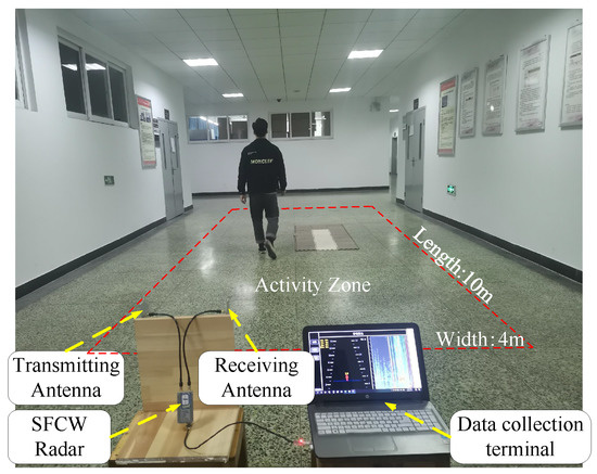
Figure 1.
A photograph of the experimental environment.
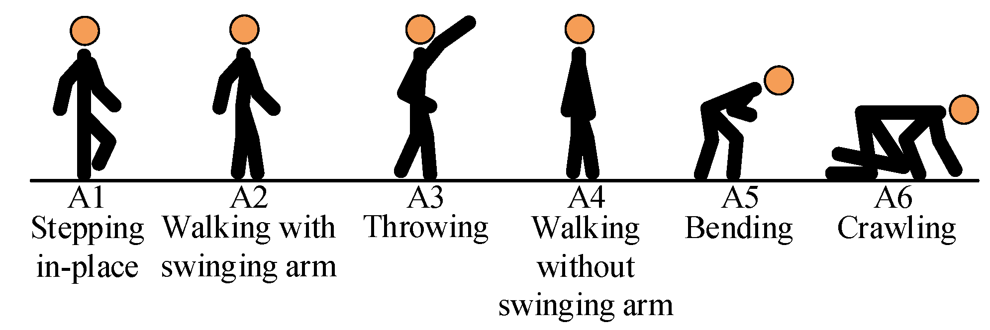
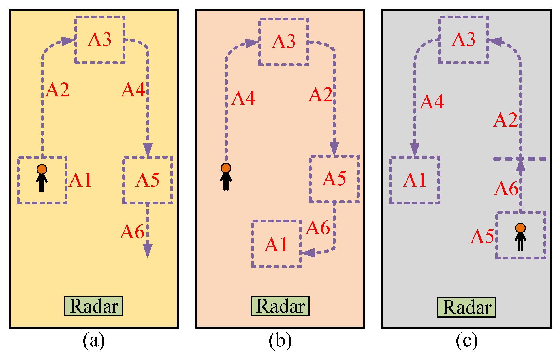
As shown in Figure 2, six typical human activities which occur frequently in real life, namely stepping in-place, walking with swinging arms, throwing, walking without swinging arms, bending and crawling, are considered. For the purposes of simplification, these six activities are represented by A1, A2, A3, A4, A5 and A6, respectively. In the limited region marked by red dotted line box in Figure 1, 11 volunteers continuously performed six activities with three different transitions, namely A1-A2-A3-A4-A5-A6, A4-A3-A2-A5-A6-A1, and A5-A6-A2-A3-A4-A1. For simplification, the three transitions of activity sequences are tagged as S1, S2 and S3. The trajectories of three sequences are shown in Figure 3, where different activities are distributed in different places. In a set of data, each activity lasts several seconds and the average duration of a sequence of six continuous activities is about 30 s. With regard to each sequence of six activities, two streams of data were collected by each volunteer. As a result, a total of 66 data streams were obtained to form the data set for training and testing.
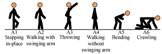
Figure 2.
Six activity models in data collection.
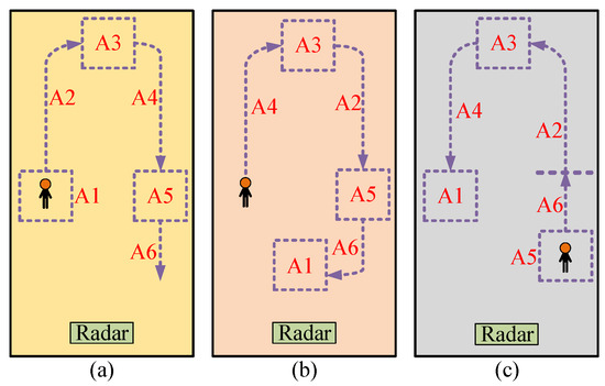
Figure 3.
Trajectory of three groups of motion sequences, (a–c) correspond to S1, S2, and S3.
2.2. Multi-Frequency Spectrogram Formation Based on Frequency-Division Processing
Assuming that a data stream is composed of L periods of SFCW radar echoes for a sequence of six activities, it is represented by a data matrix of 301 rows (frequency number) and L columns (period number) as shown in Figure 4. Obviously, each row of vectors is able to be regarded as a data vector of single-frequency continuous-wave radar. Therefore, from the perspective of rows, the data matrix is considered as data vectors of 301 different frequencies.
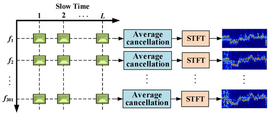
Figure 4.
Diagram of frequency-division processing.
As shown in Figure 4, the proposed frequency-division processing strategy is performed along each row to generate multiple spectrograms at different frequencies. Specifically, in the first step, the strong stationary clutters such as transmitting–receiving direct wave and ground clutters are suppressed by average cancellation which subtracts the mean value of a data row. Then, STFT is adopted to convert the data row into the spectrogram at the corresponding single frequency. For example, corresponding to m-th row of data, the spectrogram at m-th frequency is calculated as
where is the data in the m-th row and the -th column, represents the sliding window function, and N is the length of STFT. In this paper, a Hamming window with a length of is selected and the sliding step is set to 1 (namely the data length of overlapping is 31). After that, a single-frequency spectrogram with the length of is formed.
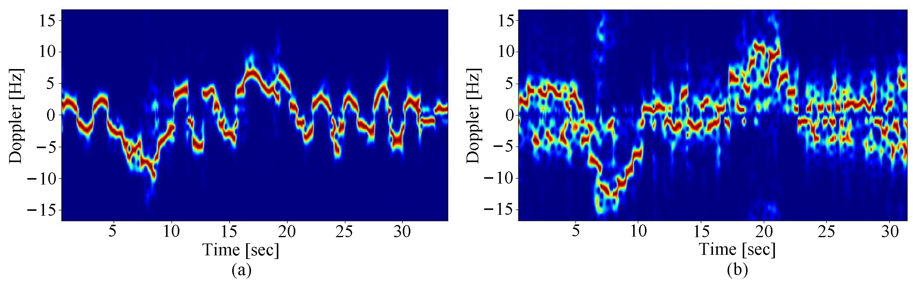
Figure 5a shows the spectrogram obtained by a rigid target. Between 0 and 4 s, the rigid target swings in situ, resulting in the frequency near zero frequency. From 4 to 10 s, the rigid target moves away from the radar, which causes that Doppler frequency shifts to the negative frequency. Within the scope of 10 to 15 s, the rigid target swings greatly in situ far from the starting point, so its frequency varies near zero frequency. The rigid target moves close to the radar between 15 and 20 s, which leads to the positive frequency in this scope. Then, from 20 s to the end, the rigid target swings in situ, causing the frequency changes near zero frequency. Similarly, Figure 5b demonstrates spectrogram of the human doing the same activity sequence. It can be seen that the spectrogram contains more Doppler information as the human body has multiple scattering points.
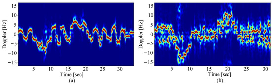
Figure 5.
The spectrogram obtained by (a) a rigid target and (b) a person.
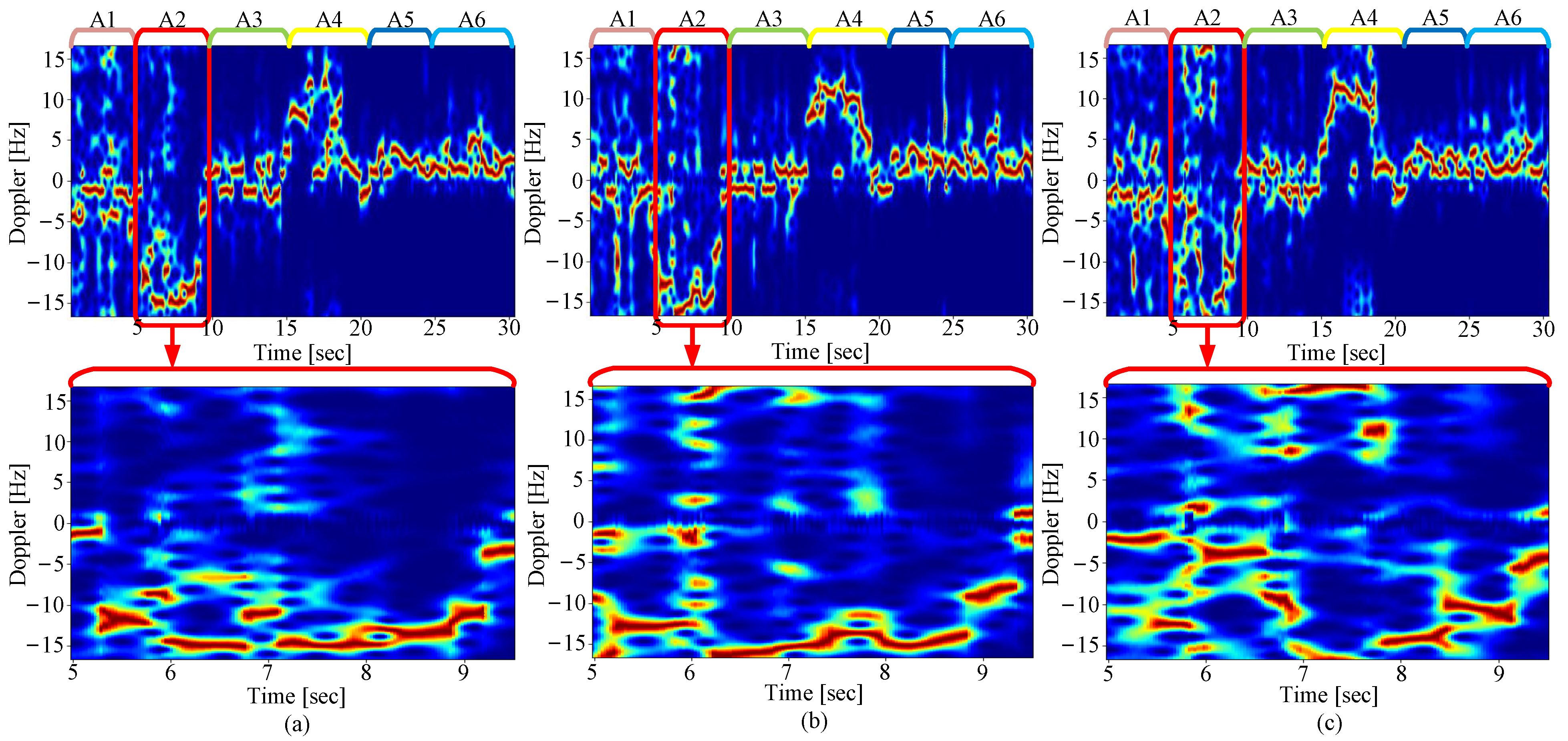
Through the frequency-division processing, a data stream for six continuous activities is transformed into 301 spectrograms at the corresponding 301 frequencies, so a data set including multi-frequency spectrograms is obtained from all the data streams. In order to obtain more clearer and obvious features, each column of the spectrogram is normalized. Figure 6 displays three samples of spectrograms at three different frequencies, namely 1.7 GHz, 1.9 GHz and 2.1 GHz. On the whole, all six activities gives different time-frequency distribution characteristics in the spectrograms of three frequencies, as shown in the top three sub-figures, which has the capability of representing human activity more comprehensively. That is because different frequencies give rise to different scattering features and frequency resolutions in the spectrograms. This phenomenon is signified more clearly from the partially zoomed spectrograms for activity A2 in the bottom three sub-figures.
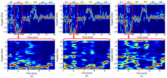
Figure 6.
Spectrograms at (a) 1.7 GHz, (b) 1.9 GHz and (c) 2.1 GHz, where the top three sub-figures are global spectrograms of six continuous activities and the bottom three sub-figures are partially zoomed spectrograms of single activity A2.
3. Model and Method
To take full advantage of the information of the time-frequency spectrogram with multi-frequency obtained above, a parallel LSTM network based on a time-frequency spectrogram with multi-frequency is designed. The network is composed of n sub-networks (each sub-network is a LSTM network based on the time-frequency spectrogram at single frequency), and the overall block diagram of the network is shown in Figure 7, where FC represents the fully connected layer and output PM denotes the output probability matrix.
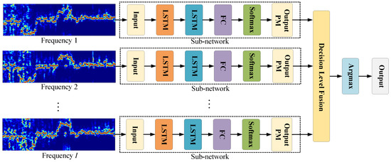
Figure 7.
Diagram of parallel LSTM network.
First of all, the sub-networks are trained with spectrograms at different frequencies, respectively. Subsequently, all sub-networks are merged to obtain the final output of the entire network. The radar spectrogram has different scattering characteristics and spatial resolutions related to human activity at different frequencies. As a result, exploring the information of time-frequency spectrograms with multiple frequencies can reflect the characteristics more completely.
3.1. The Cell Structure of Uni-LSTM and Bi-LSTM
For the purpose of extracting the characteristics in the spectrogram of continuous activity, two neural cells (namely Uni-LSTM and Bi-LSTM) are used in the experiment. Compared with other neural cells, as these two kinds of cells are capable of dealing with the problem of long-term dependence in the sequence commendable, they are particularly suitable for continuous HAR. Additionally, the model outputs a recognition result for each column of the time-frequency spectrogram through LSTM, which makes the method immune to the activity duration, spares from activity segmentation, and has high flexibility and strong adaptability.
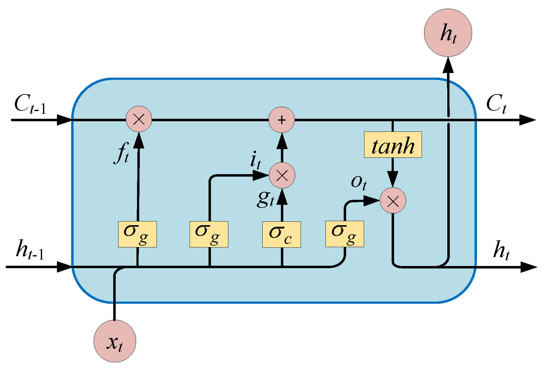
The internal structure of the Uni-LSTM is shown in Figure 8. It consists of forget gate, input gate, output gate, and cell gate, with their corresponding outputs , , and which are given by
in these formulas, represents sigmoid activation function, while is hyperbolic tangent activation function. denotes the output state at the previous moment. indicates the input at current time. W and b stand for the weight matrix and offset matrix, respectively.
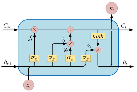
Figure 8.
Structure of Uni-LSTM cell.
In these four parts, the forget gate chooses to keep the useful information in based on and , the input gate and the cell gate are used for extracting the information in and together, and the output gate is applied to determine the output of the cell based on and . According to these four parts, the cell state and output of the Uni-LSTM cell are obtained as
where means the cell state of the previous cell. It can be seen from (6) that the cell state is determined by the and the input at the current moment, and it records all the previous useful information. Therefore, the Uni-LSTM cell has the function of long-term information memory.
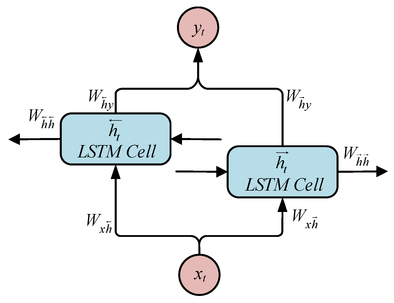
Uni-LSTM cell merely extracts forward information, while Bi-LSTM cells cope with the data in two directions through two separate Uni-LSTM cells. Then, forwarding the output of the two cells to the output layer of the Bi-LSTM unit achieves the extraction of bidirectional information. The cell structure of Bi-LSTM is shown in Figure 9. The forward channel output , the backward channel output , and the output of the whole cell of the Bi-LSTM cell are listed as follows
where the forward and backward arrows denote the parameters of the forward and backward Uni-LSTM cell. represents the weight matrix of the Uni-LSTM cell to the input, symbolizes the weight matrix of the current Uni-LSTM cell to the next cell, represents the weight matrix of the Uni-LSTM cell output to the Bi-LSTM cell, and signifies the hyperbolic tangent activation function. In the end, the output of the Bi-LSTM unit realizes the extraction of bidirectional information by fusing the output of Uni-LSTM in two directions.
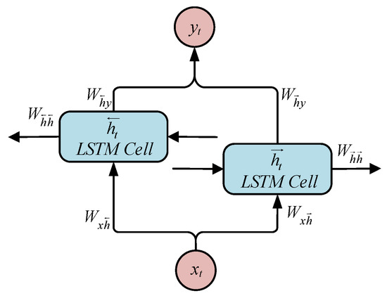
Figure 9.
Structure of Bi-LSTM cell.
3.2. Network Fusion Strategy and Label Recognition Method
For the decision level fusion layer, it is presumed that the total time length of the input data is T, and the input data contains a total of J activities. A probability matrix of size is obtained after inputting the data into the sub-network. For each probability matrix based on the output of a single frequency sub-network, the fusion strategy is
where represents the probability matrix output after the model is fused by the decision level, I is the number of frequencies that the input network fuses, stands for the probability matrix output of the i-th sub-network, and indicates the probability of tag J corresponding to the T-th frame input data of the i-th sub-network.
After the network is merged, a probability matrix whose size is same as that of sub-network is finally output. It is composed of multiple J-dimensional column vectors, and each column vector represents a probability vector output by the network at a time. It can be seen from the fusion strategy that the largest probability component in the probability vector is the label accquired by the model, and the network obtains the classification label of the sequence from the probability matrix as:
where is a vector, which means the identified probability vector by the spectrogram information of a i-th frame. The operation means taking out the row subscript of the maximum value in the vector, and the prediction label from the classifier is obtained by taking out its subscript label. After calculation, a row vector of length T is obtained, which is the prediction label of the sequence.
4. Experimental Results and Analyses
In the procedure of training the proposed parallelism LSTM network, each sub-network is trained independently by inputting the corresponding single-frequency spectrograms. When testing the network, the final recognition result for multi-frequency spectrograms comes from the addition fusion of the recognition result of each sub-network. The experimental results of the single-frequency sub-networks and integrated parallel multi-frequency network are compared to prove the effectiveness of exploiting multi-frequency spectrograms. Moreover, not only the performance of Uni-LSTM and Bi-LSTM networks on continuous HAR but also the performance changes of multi-frequency parallelism Bi-LSTM varying with the number of frequencies are analyzed.
In this paper, the supervised learning method is employed to train all recognition networks. Firstly, spectrograms are fed into the network to obtain the predicted label, and the cross-entropy loss function is applied to calculate the error between the truth label and the predicted label. Subsequently, the network parameters are optimized by Adam optimizer with a learning rate of 0.001, and the drop-out function is used to prevent over-fitting. In order to implement cross-validation, the data set is divided into the training set and the testing set by a ratio of ten to one. The networks are trained on TensorFlow which is an open-source deep-learning toolkit. At the same time, NVIDIA RTX 3090 GPU and CUDA library are utilized to accelerate the training process.
4.1. Uni-LSTM Sub-Network for Single-Frequency Spectrogram
As shown in the Figure 7, the sub-network consists of two cascade Uni-LSTM modules, a fully connected layer and a softmax classifier. The parameters of the sub-network are shown in Table 1.

Table 1.
Parameters and properties of Uni-LSTM sub-network and Bi-LSTM sub-network.
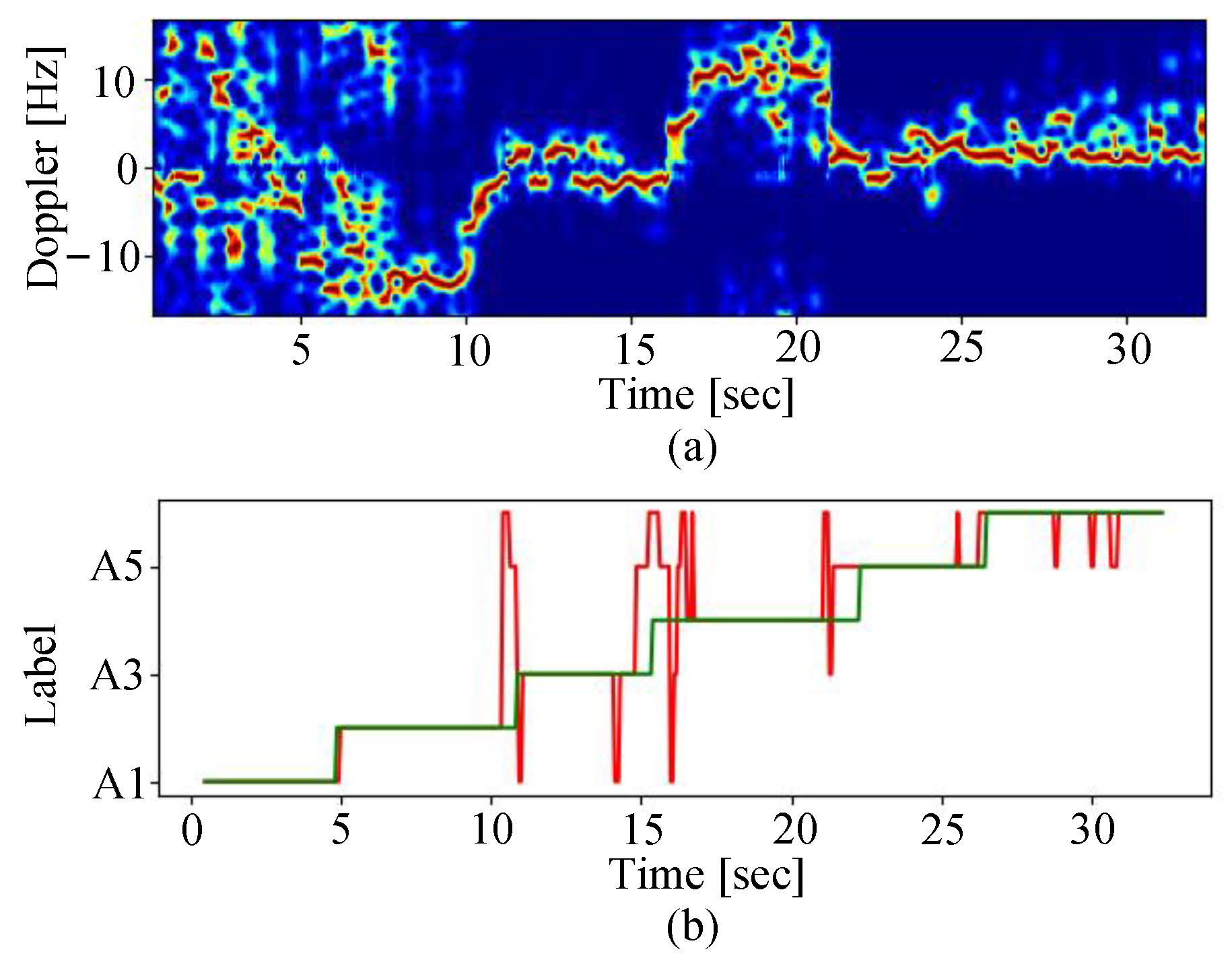
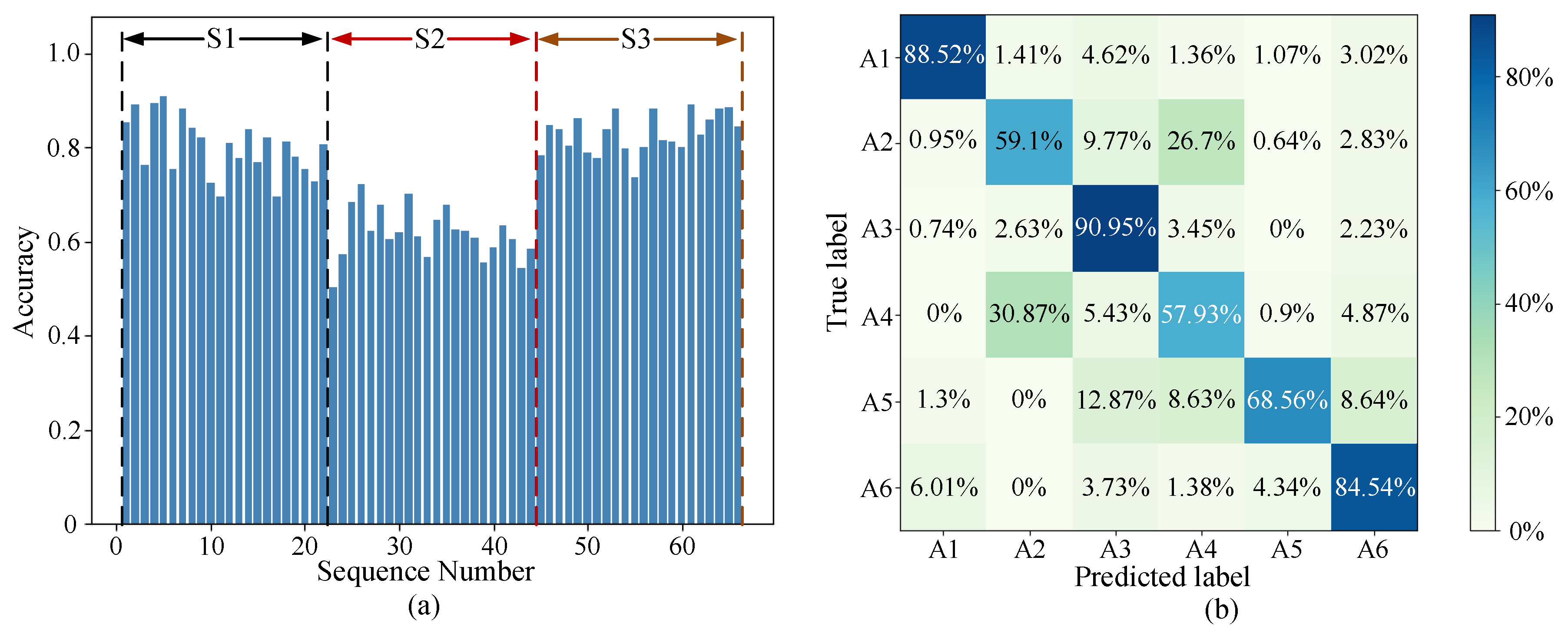
Based on the trained Uni-LSTM sub-network, Figure 10b shows the recognition results of the single-frequency spectrogram at 1.7 GHz, which are displayed in Figure 10a. In this sample, six activities are performed by following the sequence S1 with the transition of A1-A2-A3-A4-A5-A6. In Figure 10b, the red line represents the recognized labels, and the green line denotes the real labels. The overlapping parts are indicated by green, meaning accurate activity recognition. The displacements of the red recognized labels illustrate that the classifier wrongly regards the spectrogram at the corresponding moments as another activity categories. It can be seen that the false recognition mainly occurs in the unstable stage of activity conversion. The recognition accuracy of this sample is 85.5%. Through a cross-validation, the recognition accuracies for all 66 single-frequency spectrograms are shown in Figure 11a, and the average accuracy is calculated as 74.99%.

Figure 10.
(a) The spectrogram of S1 at 1.7 GHz. (b) The corresponding recognition result using a trained Uni-LSTM sub-network, where green and red lines represent real and identified labels.
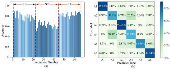
Figure 11.
(a) Recognition performance; (b) confusion matrix of Uni-LSTM sub-network at 1.7 GHz spectrogram.
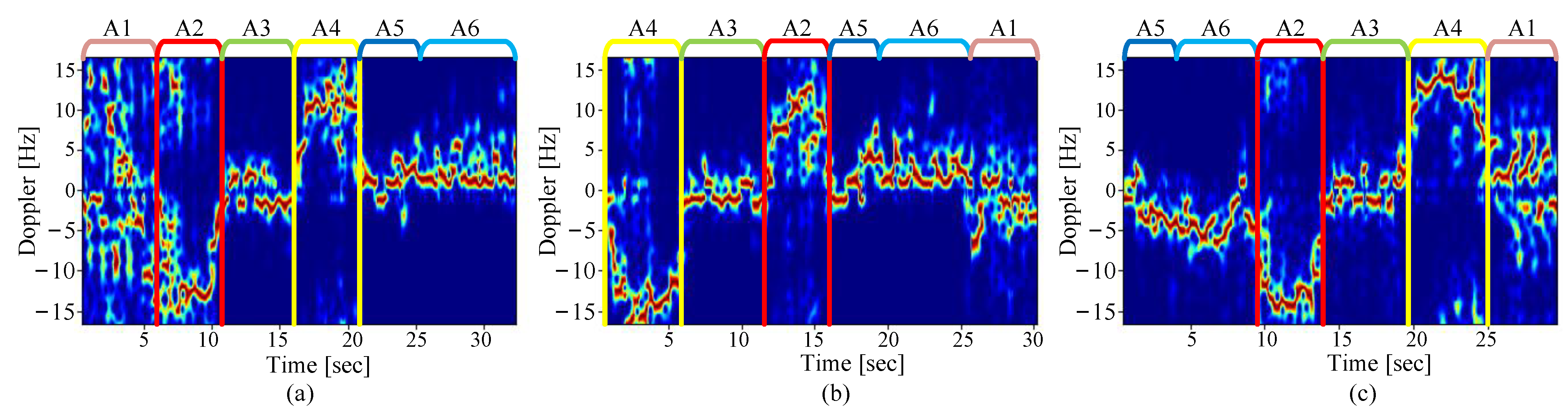
As can be seen from Figure 11a, the recognition accuracy of sequence S2 is much lower than that of S1 and S3. On the one hand, A2 and A4 are difficult to distinguish for their similarity in movement. As there is high similarity of the spectrogram between A2 and A4 shown in Figure 12, and the spectrogram has a low resolution for detailed actions at 1.7 GHz, there is serious confusion between the activities of A2 and A4 which corresponds to Figure 11b. On the other hand, the difference between S1, S3 and S2 also makes A2 and A4 in S2 more confused. Since moving directions of A2 and A4 are opposite to those in S1 and S3, the main frequency of A2 and A4 in S2 are reversed from that in S1 and S3, as shown in Figure 12. As a result, for the total samples training the network, the sample number of A2 in the negative frequency is significantly more than A2 in the positive frequency, while A4 shows a contrary phenomenon. Therefore, the network prefers to recognize A2 with positive frequency in S2 as A4, while regards A4 with negative frequency as A2.

Figure 12.
The spectrogram of the sequences (a) S1, (b) S2 and (c) S3.
4.2. Uni-LSTM Sub-Network Based on Spectrogram of Different Frequencies
As can be seen from Figure 6, there are different characteristic distribution on the spectrograms of different frequencies for the same activity of the same data, which is experessed as different recognition performance. In order to verify this inference, the same method as that in Section 4.1 is exploited to recognize the continuous human activity on the spectrograms of five different frequencies (1.7 GHz, 1.8 GHz, 1.9 GHz, 2.0 GHz and 2.1 GHz) obtained in Section 2.2.
The recognition performance of the network on the spectrogram of five different frequencies is shown in Figure 13. In this figure, five sub-graphs represent the recognition accuracy of the model at five frequencies. It can be seen from the figure that the network exhibits different recognition performances at different frequencies. Table 2 shows the average recognition accuracy of the sub-networks at the five frequencies. After a comprehensive analysis of Figure 13 and Table 2, compared with the two low frequencies, the recognition accuracy at a high frequency on all sequences is more uniform, the average recognition accuracy of a high frequency is about 5% higher than that of a low frequency.
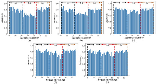
Figure 13.
Recognition performance of Uni-LSTM sub-network on five frequencies, namely (a) 1.7 GHz, (b) 1.8 GHz, (c) 1.9 GHz, (d) 2.0 GHz, (e) 2.1 GHz.
Table 2.
The average accuracy of the LSTM network over 5 frequencies.
4.3. Decision Level Fusion of Parallelism Uni-LSTM
In previous studies, continuous HAR is mainly realized by using single-frequency micro-Doppler features. As is mentioned above, for a single frequency, there is worse confusion in the recognition of the two similar activities. It can be seen from Section 4.2 that the sub-network has different recognition performance on the spectrogram of different frequencies. Therefore, the fusion of the decision level of the parallelism LSTM with a multi-frequency spectrogram is proposed, as shown in Figure 7. At the beginning, spectrograms at five frequencies are employed to train the Uni-LSTM sub-network structure the same as Section 4.1. Then, the output probability matrices of each sub-network are fused by (11) to gain the final probability matrix output. After that, the human activity label is acquired by using (12).
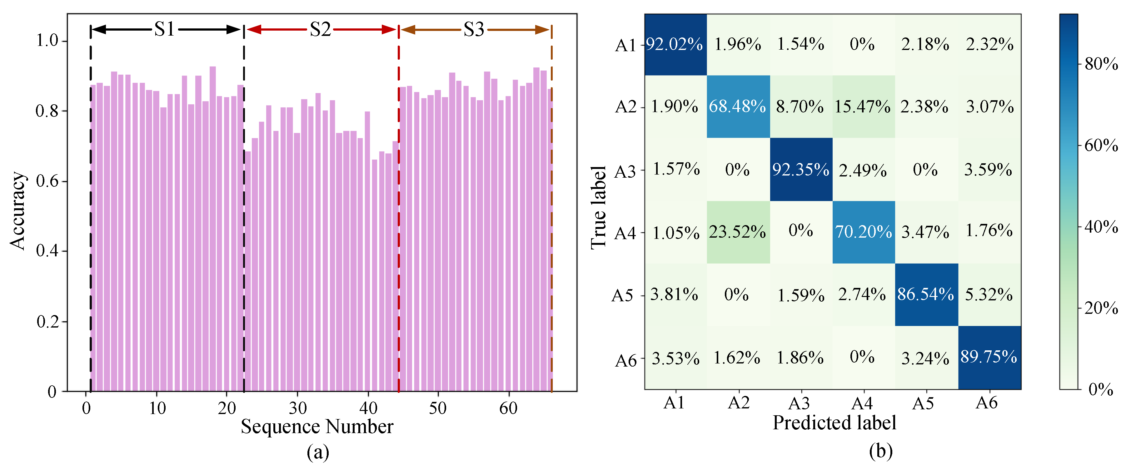
The comparison between the single-frequency Uni-LSTM prediction label and parallelism Uni-LSTM with multi-frequency prediction label is shown in Figure 14, which shows that the method based on fusion significantly achieves higher classification accuracy. Additionally, the recognition accuracy of each sequence after fusion is shown in Figure 15a. After statistics, the average recognition accuracy after fusion reaches 85.41%, which is improved by about 5% compared with the single-frequency sub-network. At the same time, it can be seen from Figure 15b that the fusion has improved the recognition accuracy of action A2 and action A4.
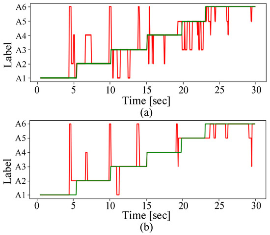
Figure 14.
Comparison of (a) single-frequency Uni-LSTM prediction label and (b) parallelism Uni-LSTM with multi-frequency prediction label.

Figure 15.
(a) The recognition accuracy and (b) confusion matrix of Uni-LSTM after multi-frequency fusion.
4.4. Performance Analysis of Bi-LSTM Network before and after Multi-Frequency Fusion
As described in Section 3.1, compared with the Uni-LSTM network, the Bi-LSTM has an advantage of using forward and backward information for recognition.
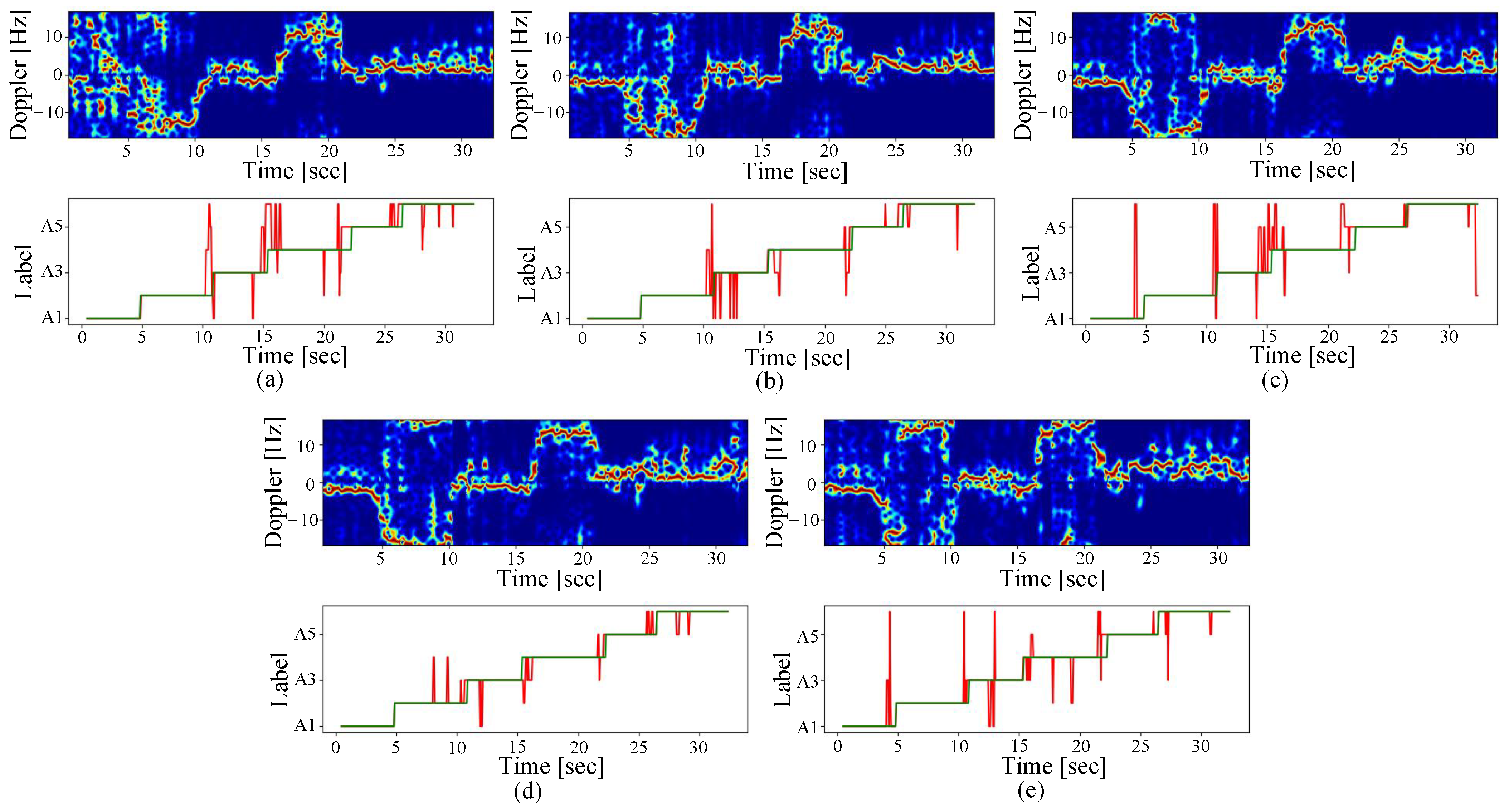
Firstly, the Uni-LSTM cell is replaced by Bi-LSTM in the network model described in Section 4.1 to obtain the Bi-LSTM sub-network based on single-frequency. The parameters of this sub-network are shown in Table 1. Futhermore, the same verification method as before is applied to attest the recognition performance of this model. Figure 16 shows the recognition results of five sub-networks on a set of data of the sequence S1, wherein each sub-graph corresponds to a recognition result on a frequency. It can be seen from the figure that although the Bi-LSTM network utilizes information in both directions for predicting, the model still has misrecognition. The recognition accuracy at the five frequencies shown in the Figure 16 are 87.38%, 91.52%, 89.26%, 92.46% and 91.33%. The test accuracy obtained from the entire data set at each frequency and the average accuracy of Bi-LSTM network are shown in Figure 17 and Table 3.
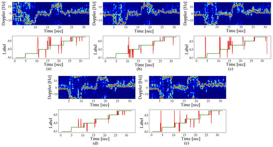
Figure 16.
Bi-LSTM resulted Doppler images and the corresponding labels in sequence S1 at the five frequencies, namely (a) 1.7 GHz, (b) 1.8 GHz, (c) 1.9 GHz, (d) 2.0 GHz, (e) 2.1 GHz.
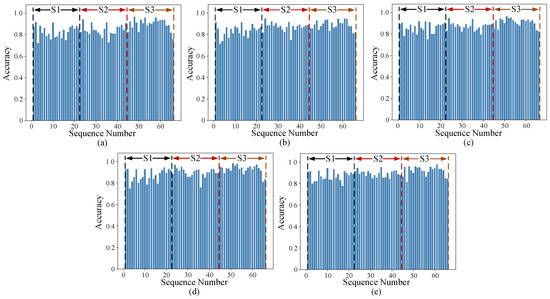
Figure 17.
Recognition accuracy of the Bi-LSTM sub-network on five frequencies, namely (a) 1.7 GHz, (b) 1.8 GHz, (c) 1.9 GHz, (d) 2.0 GHz, (e) 2.1 GHz.
Table 3.
Average recognition accuracy of Bi-LSTM network at five frequencies.
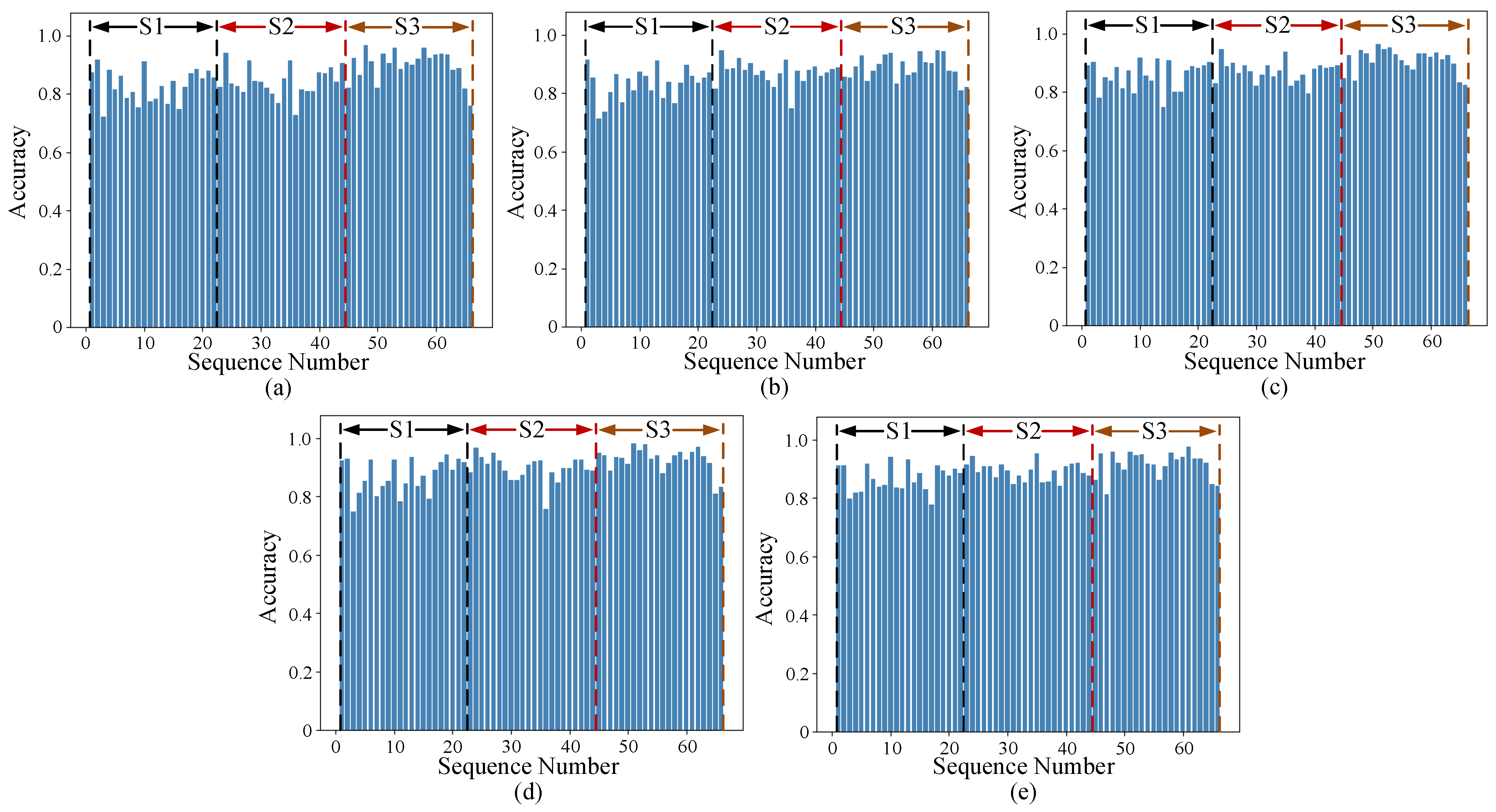
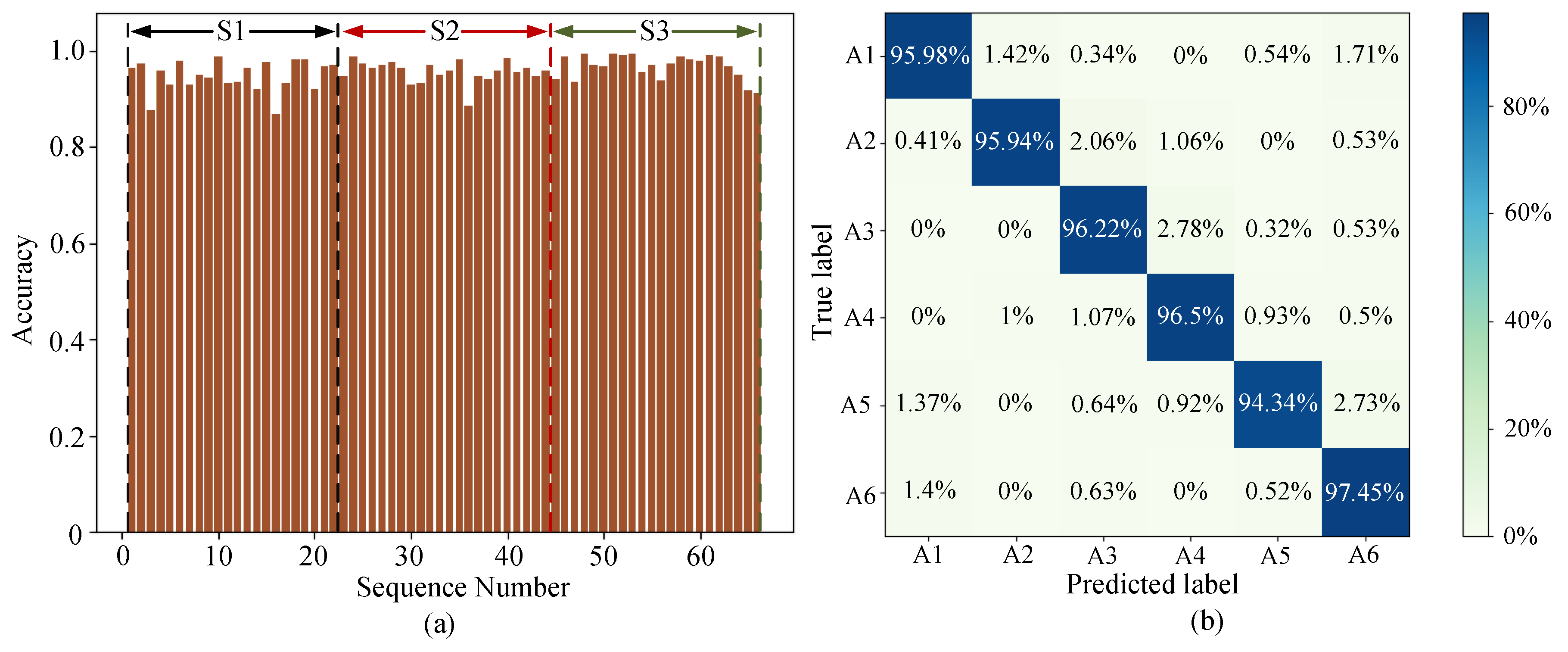
In order to verify the proposed multi-frequency fusion network model based on Bi-LSTM, the same method as Section 4.3 is exploited to realize continuous HAR. The network model is obtained by replacing the Uni-LSTM cell in Figure 7 with a Bi-LSTM cell. Based on the trained Bi-LSTM network, Figure 18 shows the recognition result of a set of data for the sequence S1. Figure 18a shows the recognition result of Bi-LSTM sub-network at 1.7 GHz, and Figure 18b exhibits the identification result of parallel multi-frequency Bi-LSTM network. From the predicted label, it is obvious that the false recognition rate is significantly reduced after multi-frequency fusion. Simultaneously, the recognition rate of the sequence reaches 96.61%. Figure 19 demonstrates the recognition accuracy and confusion matrix of the parallel multi-frequency Bi-LSTM network on the entire data set. As can be seen from Figure 19b, the recognition performance of Bi-LSTM network with multi-frequency fusion is further improved, and the average recognition accuracy of the model reaches 96.15%. Additionally, it is obvious that the network misrecognition is greatly reduced from the confusion matrix of Figure 19b.

Figure 18.
Comparison of (a) single-frequency Bi-LSTM prediction label and (b) parallelism Bi-LSTM with multi-frequency prediction label.
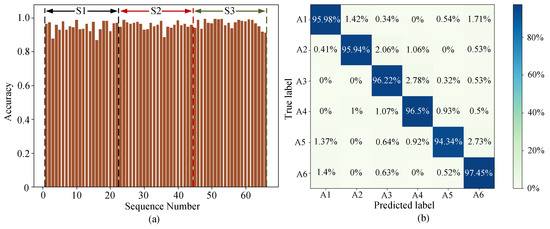
Figure 19.
(a) The recognition accuracy and (b) confusion matrix of Bi-LSTM after multi-frequency fusion.
4.5. Performance Analysis on Variable Numbers of Multi-Frequency Fusion and Variant Learning Rate
Through the above experiments, it can be seen that the utilization of multi-frequency fusion is conducive to effectively improving the accuracy of continuous HAR. In this section, the Bi-LSTM network is used to analyze the specific impact of the number of different frequency spectrograms on the network recognition accuracy.
In Figure 20, for one frequency, 1.7 GHz is selected for experiment, while for multi-frequency fusion, the method of sampling on 301 frequencies with the equal frequency interval is adopted. For example, in the analysis of two frequencies, 1.6 GHz and 2.2 GHz are chosen. When the number of frequency points is three, 1.6 GHz, 1.9 GHz and 2.2 GHz are opted. The experimental results show that when the number of fusion frequencies exceeds 4, the improvement of network performance is not obvious. In addition, with the increase in the number of fusion frequencies, the network structure is becoming more and more complex, and the computation burden is increasing as well. As a result, five frequencies are used for fusion in this paper.

Figure 20.
Accuracy and performance improvement rate of variable numbers of multi-frequency after fusing.
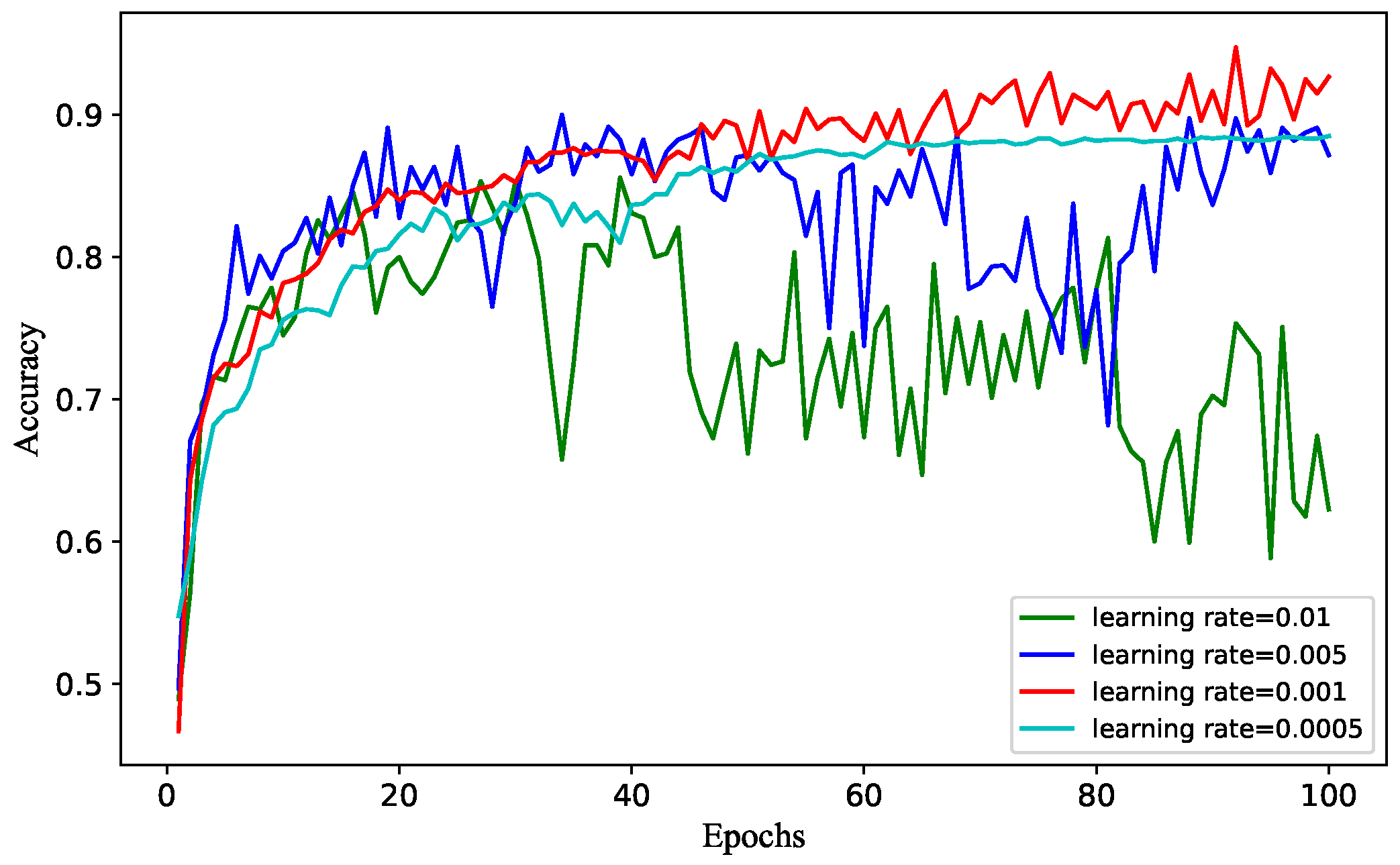
Figure 21 shows the recognition accuracy of Bi-LSTM sub-network trained according to different learning rates on the data set. Its parameters are shown in Table 1. Cross-entropy loss function is utilized to calculate the loss, while Adam is selected as optimizer. The results are obtained by training the network with the learning rates of 0.01, 0.005, 0.001 and 0.0005, respectively. It can be seen from the curves that when the learning rate is large, the accuracy of the network is still unable to improve after multiple rounds of training. If the learning rate is small, the network training becomes slow, and the accuracy fails to be further improved when it reaches a certain value. Therefore, the learning rate used in the experiment is 0.001.
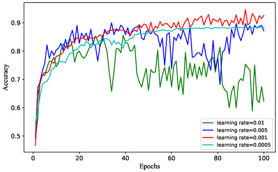
Figure 21.
The recognition accuracy of Bi-LSTM sub-network with different learning rates.
4.6. Performance Comparison of the Three Models
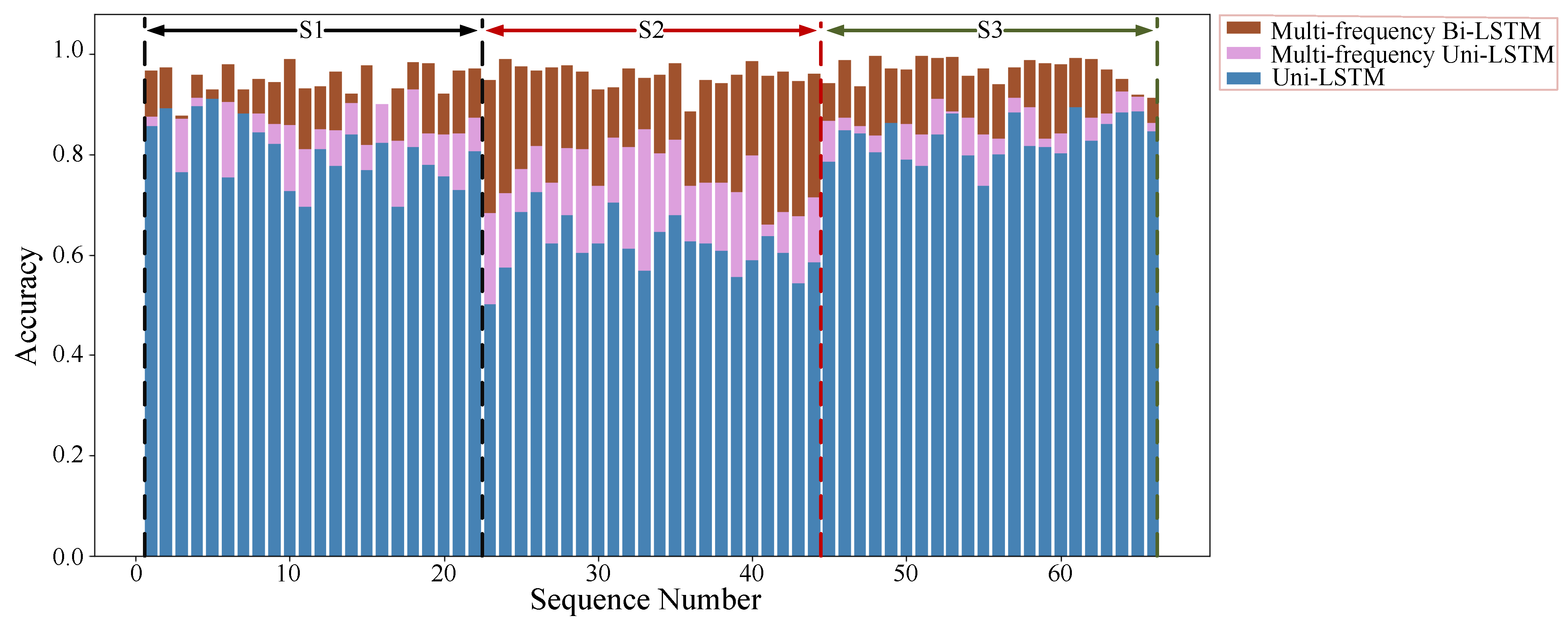
The comparison chart of the test accuracy of the three models on the data set is shown in Figure 22. By comparing the recognition accuracy of the Uni-LSTM and the parallelism Uni-LSTM with multi-frequency spectrograms, it can be observed that the accuracy of fusion is slightly improved in sequence S1 and sequence S3. Additionally, the final prediction accuracy in sequence S2 after fusion greatly improves due to the fusion of multi-frequency spectrograms. Compared with the accuracy at 1.7 GHz, the average accuracy of multi-frequency fusion LSTM is improved by 10.42%. The comparison between the parallelism Uni-LSTM and Bi-LSTM with multi-frequency spectrograms shows that the recognition accuracy of Bi-LSTM network for S1, S2 and S3 has different degrees of optimization and improvement. The overall average recognition accuracy increases by 10.74%.
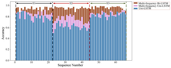
Figure 22.
Comparison of recognition accuracy of the three models.
5. Discussion
HAR is a research focus in the field of machine perception and pattern recognition, which classifies human activity according to the characteristics of input data. In the research of HAR based on radar, the activity required to identify the data types of human activity and the design of the network model have a crucial impact on the recognition performance. Previous studies mostly research the recognition of a single activity, which only extracts the characteristics within single human activity without the information of the conversion between activities. However, as people act freely and continuously in real life, discrete HAR lacks wide application value. Therefore, few studies have began to conduct continuous HAR recently. In [47], a Bi-LSTM network is designed to extract the forward and backward features related to continuous HAR from the time-frequency spectrogram, achieving a satisfactory result. Based on this work, inspired by ensemble learning, and considering frequency-division characteristics of SFCW radar, we design a parallel LSTM network to obtain the feature of a multi-frequency spectrogram, and integrate the outputs of sub-networks to improve the recognition performance.
In the experiment, an SFCW radar is used to collect data of human activity sequence which includes six activities. Firstly, the Uni-LSTM [47] based on the single-frequency data is verified with the highest average recognition accuracy of 80.6%. On this basis, multi-frequency spectrograms are experimented on Uni-LSTM, and the accuracy is 85.41%. Compared with the recognition result of single frequency, the accuracy is improved by 4.81%. Subsequently, the above experiment is repeated under the condition that the layer Uni-LSTM is replaced by Bi-LSTM. The highest average recognition accuracy of Bi-LSTM with single-frequency spectrogram reaches 89.82%, while it is 95.15% with multi-frequency fusion, which indicates that the accuracy improves more than 5%. In summary, as multi-frequency fusion introduces different scattering properties and frequency resolutions, the expression of the human activity feature is more abundant, so that the proposed recognition method significantly improves the accuracy of HAR, which provides a reference for other scholars to research continuous HAR.
In addition, the network mentioned in this paper only verifies the data of six collected activities. In future research work, more activities are needed to further explore radar-based HAR, and the combination of other deep learning models with radar HAR is required to further promote the advance of radar-based HAR [51,52].
6. Conclusions
In this paper, a continuous HAR method based on parallelism LSTM with multi-frequency spectrograms is proposed. Multiple parallel LSTM networks are used to extract and fuse time-frequency features with different scattering characteristics and spatial resolution from a spectrogram at different frequencies, which improves the performance of continuous HAR.
More specifically, two models adopting spectrograms at five frequencies, one based on Uni-LSTM and the other using Bi-LSTM, are proposed in this paper. To prove the effectiveness of multi-frequency fusion, the parallelism LSTM using multi-frequency spectrograms is compared with a single-frequency LSTM. The results illustrate that, for the model based on Uni-LSTM, the introduction of multiple frequencies increases the accuracy by around 5%. At the same time, for the model using Bi-LSTM, the accuracy is 96.15% for the method with multiple frequencies, while it is 89.82% for the model with single frequency. Additionally, the influence of the number of frequencies in multi-frequency fusion is analyzed. The experimental results show that the recognition accuracy tends to be stable when the number of input frequencies reaches four.
There are still some limitations in the proposed method. In practical applications, as the proposed method is based on multi-frequency analysis, it is limited by the type of radar equipment. The radar equipment must have the ability to obtain data at multiple frequencies. In addition, when it is required to recognize a new activity, the relevant data of the new activity are needed for retraining the model. As a result, further research is required in the future to solve those problems for a broader application.
Author Contributions
Conceptualization, C.D. and Y.J.; methodology, C.D. and G.C.; software, validation, formal analysis, C.D. and Y.J.; data curation, writing—original draft preparation, C.D., Y.J. and C.C.; writing—review and editing, funding acquisition, Y.J., G.C., X.Z. and Y.G. All authors have read and agreed to the published version of the manuscript.
Funding
This work is supported financially by Sichuan Science and Technology Program under Grant 2020YFG0170 and 2020YFG0169, and National Natural Science Foundation of China under Grants 61871080 and 41574136.
Data Availability Statement
The data presented in this study are available on request from the corresponding author.
Acknowledgments
The authors acknowledge the above funds for supporting this research and editor and reviewers for their comments and suggestions.
Conflicts of Interest
The authors declare no conflict of interest.
References
- Muhammad, K.; Mustaqeem; Ullah, A.; Imranb, A.S.; Sajjad, M.; Kiran, M.S.; Sannino, G.; de Albuquerque, V.H.C. Human action recognition using attention based LSTM network with dilated CNN features. Future Gener. Comput. Syst. 2021, 125, 820–830. [Google Scholar] [CrossRef]
- Stove, A.G.; Sykes, S.R. A doppler-based automatic target classifier for a battlefield surveillance radar. In Proceedings of the IET Conference Proceedings, Edinburgh, UK, 15–17 October 2002; pp. 419–423. [Google Scholar]
- Yang, X.; Zhang, X.; Ding, Y.; Zhang, L. Indoor Activity and Vital Sign Monitoring for Moving People with Multiple Radar Data Fusion. Remote Sens. 2021, 13, 3791. [Google Scholar] [CrossRef]
- Li, G.; Zhang, R.; Ritchie, M.; Griffiths, H. Sparsity-driven micro-doppler feature extraction for dynamic hand gesture recognition. IEEE Trans. Aerosp. Electron. Syst. 2018, 54, 655–665. [Google Scholar] [CrossRef]
- Mukhopadhyay, S.C. Wearable sensors for human activity monitoring: A review. IEEE Sens. J. 2015, 15, 1321–1330. [Google Scholar] [CrossRef]
- Chaccour, K.; Darazi, R.; El Hassani, A.H.; Andrès, E. From fall detection to fall prevention: A generic classification of fall-related systems. IEEE Sens. J. 2017, 17, 812–822. [Google Scholar] [CrossRef]
- Zhu, C.; Sheng, W. Wearable sensor-based hand gesture and daily activity recognition for robot-assisted living. IEEE Trans. Syst. Man Cybern.-Part A Syst. Humans 2011, 41, 569–573. [Google Scholar] [CrossRef]
- Luo, F.; Poslad, S.; Bodanese, E. Human activity detection and coarse localization outdoors using micro-doppler signatures. IEEE Sens. J. 2019, 19, 8079–8094. [Google Scholar] [CrossRef]
- Wang, H.; Zhang, D.; Wang, Y.; Ma, J.; Wang, Y.; Li, S. RT-Fall: A real-time and contactless fall detection system with commodity WiFi devices. IEEE Trans. Mob. Comput. 2017, 16, 511–526. [Google Scholar] [CrossRef]
- Amin, M.G.; Zhang, Y.D.; Ahmad, F.; Ho, K.C.D. Radar signal processing for elderly fall detection: The future for in-home monitoring. IEEE Signal Process. Mag. 2016, 33, 71–80. [Google Scholar] [CrossRef]
- Alfuadi, R.; Mutijarsa, K. Classification method for prediction of human activity using stereo camera. In Proceedings of the 2016 International Seminar on Application for Technology of Information and Communication (ISemantic), Semarang, Indonesia, 5–6 August 2016; pp. 51–57. [Google Scholar]
- Zin, T.T.; Tin, P.; Hama, H.; Toriu, T. Unattended object intelligent analyzer for consumer video surveillance. IEEE Trans. Consum. Electron. 2011, 57, 549–557. [Google Scholar] [CrossRef]
- Li, Z.; Jin, T.; Dai, Y.; Song, Y. Through-Wall Multi-Subject Localization and Vital Signs Monitoring Using UWB MIMO Imaging Radar. Remote Sens. 2021, 13, 2905. [Google Scholar] [CrossRef]
- Narayanan, R.M.; Zenaldin, M. Radar micro-Doppler signatures of various human activities. IET Radar Sonar Navig. 2015, 9, 1205–1215. [Google Scholar] [CrossRef]
- Kumar, D.; Sarkar, A.; Kerketta, S.R.; Ghosh, D. Human activity classification based on breathing patterns using IR-UWB radar. In Proceedings of the 2019 IEEE 16th India Council International Conference (INDICON), Rajkot, India, 13–15 December 2019; pp. 1–4. [Google Scholar]
- Sasakawa, D.; Honma, N.; Nakayama, T.; Iizuka, S. Human activity identification by height and doppler RCS information detected by MIMO radar. IEICE Trans. Commun. 2019, E102.B, 1270–1278. [Google Scholar] [CrossRef]
- Lee, D.; Park, H.; Moon, T.; Kim, Y. Continual learning of micro-Doppler signature-based human activity classification. IEEE Geosci. Remote. Sens. Lett. 2021, 1–5. [Google Scholar] [CrossRef]
- Kim, Y.; Ling, H. Human activity classification based on micro-Doppler signatures using a support vector machine. IEEE Trans. Geosci. Remote Sens. 2009, 47, 1328–1337. [Google Scholar]
- Lin, Y.; Le Kernec, J. Performance analysis of classification algorithms for activity recognition using micro-Doppler feature. In Proceedings of the 2017 13th International Conference on Computational Intelligence and Security (CIS), Hong Kong, China, 15–18 December 2017; pp. 480–483. [Google Scholar]
- Markopoulos, P.P.; Zlotnikov, S.; Ahmad, F. Adaptive radar-based human activity recognition with L1-Norm linear discriminant analysis. IEEE J. Electromagn. RF Microwaves Med. Biol. 2019, 3, 120–126. [Google Scholar] [CrossRef]
- Li, X.; He, Y.; Jing, X. A survey of deep learning-based human activity recognition in radar. Remote Sens. 2019, 11, 1068. [Google Scholar] [CrossRef] [Green Version]
- Jokanovic, B.; Amin, M.; Ahmad, F. Radar fall motion detection using deep learning. In Proceedings of the 2016 IEEE Radar Conference (RadarConf), Philadelphia, PA, USA, 2–6 May 2016; pp. 1–6. [Google Scholar]
- Vandersmissen, B.; Knudde, N.; Jalalvand, A.; Couckuyt, I.; Dhaene, T.; De Neve, W. Indoor human activity recognition using high-dimensional sensors and deep neural networks. Neural Comput. Appl. 2020, 32, 12295–12309. [Google Scholar] [CrossRef]
- Qiao, X.; Shan, T.; Tao, R. Human identification based on radar micro-Doppler signatures separation. Electron. Lett. 2020, 56, 155–156. [Google Scholar] [CrossRef]
- Kim, Y.; Moon, T. Human detection and activity classification based on micro-Doppler signatures using deep convolutional neural networks. IEEE Geosci. Remote Sens. Lett. 2016, 13, 8–12. [Google Scholar] [CrossRef]
- Li, X.; He, Y.; Yang, Y.; Hong, Y.; Jing, X. LSTM based human activity classification on radar range profile. In Proceedings of the 2019 IEEE International Conference on Computational Electromagnetics (ICCEM), Shanghai, China, 20–22 March 2019; pp. 1–2. [Google Scholar]
- Wang, M.; Zhang, Y.D.; Cui, G. Human motion recognition exploiting radar with stacked recurrent neural network. Digit. Signal Process. 2019, 87, 125–131. [Google Scholar] [CrossRef]
- Zhu, J.; Chen, H.; Ye, W. A hybrid CNN–LSTM network for the classification of human activities based on micro-Doppler radar. IEEE Access. 2020, 8, 24713–24720. [Google Scholar] [CrossRef]
- Shrestha, A.; Murphy, C.; Johnson, I.; Anbulselvam, A.; Fioranelli, F.; Kernec, J.L.; Gurbuz, S.Z. Cross-frequency classification of indoor activities with DNN transfer learning. In Proceedings of the 2019 IEEE Radar Conference (RadarConf), Boston, MA, USA, 22–26 April 2019; pp. 1–6. [Google Scholar]
- Seyfioglu, M.S.; Erol, B.; Gurbuz, S.Z.; Amin, M.G. DNN transfer learning from diversified micro-Doppler for motion classification. IEEE Trans. Aerosp. Electron. Syst. 2019, 55, 2164–2180. [Google Scholar] [CrossRef] [Green Version]
- Seyfioğlu, M.S.; Özbayoğlu, A.M.; Gürbüz, S.Z. Deep convolutional autoencoder for radar-based classification of similar aided and unaided human activities. IEEE Trans. Aerosp. Electron. Syst. 2018, 54, 1709–1723. [Google Scholar] [CrossRef]
- Li, X.; Jing, X.; He, Y. Unsupervised domain adaptation for human activity recognition in radar. In Proceedings of the 2020 IEEE Radar Conference (RadarConf20), Florence, Italy, 21–25 September 2020; pp. 1–5. [Google Scholar]
- Du, H.; Jin, T.; Song, Y.; Dai, Y. Unsupervised adversarial domain adaptation for micro-Doppler based human activity classification. IEEE Geosci. Remote Sens. Lett. 2020, 17, 62–66. [Google Scholar] [CrossRef]
- Mi, Y.; Jing, X.; Mu, J.; Li, X.; He, Y. DCGAN-based scheme for radar spectrogram augmentation in human activity classification. In Proceedings of the 2018 IEEE International Symposium on Antennas and Propagation & USNC/URSI National Radio Science Meeting, Atlanta, GA, USA, 7–12 July 2018; pp. 1973–1974. [Google Scholar]
- Alnujaim, I.; Oh, D.; Kim, Y. Generative adversarial networks to augment micro-Doppler signatures for the classification of human activity. In Proceedings of the IGARSS 2019 - 2019 IEEE International Geoscience and Remote Sensing Symposium, Yokohama, Japan, 28 July–2 August 2019; pp. 9459–9461. [Google Scholar]
- Jokanović, B.; Amin, M. Fall detection using deep learning in range-Doppler radars. IEEE Trans. Aerosp. Electron. Syst. 2018, 54, 180–189. [Google Scholar] [CrossRef]
- Hernangómez, R.; Santra, A.; Stańczak, S. Human activity classification with frequency modulated continuous wave radar using deep convolutional neural networks. In Proceedings of the 2019 International Radar Conference (RADAR), Toulon, France, 23–27 September 2019; pp. 1–6. [Google Scholar]
- Jia, Y.; Guo, Y.; Wang, G.; Song, R.; Cui, G.; Zhong, X. Multi-frequency and multi-domain human activity recognition based on SFCW radar using deep learning. Neurocomputing 2020, 444, 274–287. [Google Scholar] [CrossRef]
- Ye, W.; Chen, H.; Li, B. Using an end-to-end convolutional network on radar signal for human activity classification. IEEE Sens. J. 2019, 19, 12244–12252. [Google Scholar] [CrossRef]
- Chen, W.; Ding, C.; Zou, Y.; Zhang, L.; Gu, C.; Hong, H.; Zhu, X. Non-contact human activity classification using DCNN based on UWB radar. In Proceedings of the 2019 IEEE MTT-S International Microwave Biomedical Conference (IMBioC), Nanjing, China, 6–8 May 2019; pp. 1–4. [Google Scholar]
- Song, Y.; Jin, T.; Dai, Y.; Zhou, X. Through-wall human pose reconstruction via UWB MIMO radar and 3D CNN. Remote Sens. 2021, 13, 241. [Google Scholar] [CrossRef]
- Adib, F.; Hsu, C.; Mao, H.; Katabi, D.; Durand, F. Capturing the human figure through a wall. ACM Trans. Graph. 2015, 34, 219. [Google Scholar] [CrossRef]
- Zhao, M.; Liu, Y.; Raghu, A.; Zhao, H.; Li, T.; Torralba, A.; Katabi, D. Through-wall human mesh recovery using radio signals. In Proceedings of the 2019 IEEE/CVF International Conference on Computer Vision (ICCV), Seoul, Korea, 27–28 October 2019; pp. 10112–10121. [Google Scholar]
- Li, H.; Shrestha, A.; Heidari, H.; Kernec, J.L.; Fioranelli, F. Activities recognition and fall detection in continuous data streams using radar sensor. In Proceedings of the 2019 IEEE MTT-S International Microwave Biomedical Conference (IMBioC), Nanjing, China, 6–8 May 2019; pp. 1–4. [Google Scholar]
- Guendel, R.G.; Fioranelli, F.; Yarovoy, A. Derivative target line (DTL) for continuous human activity detection and recognition. In Proceedings of the 2020 IEEE Radar Conference (RadarConf20), Florence, Italy, 21–25 September 2020; pp. 1–6. [Google Scholar]
- Ding, C.; Hong, H.; Zou, Y.; Chu, H.; Zhu, X.; Fioranelli, F.; Kernec, J.L.; Li, C. Continuous human motion recognition with a dynamic range-Doppler trajectory method based on FMCW radar. IEEE Trans. Geosci. Remote Sens. 2019, 57, 6821–6831. [Google Scholar] [CrossRef]
- Shrestha, A.; Li, H.; Le Kernec, J.; Fioranelli, F. Continuous human activity classification from FMCW radar with Bi-LSTM networks. IEEE Sens. J. 2020, 20, 13607–13619. [Google Scholar] [CrossRef]
- Li, H.; Shrestha, A.; Heidari, H.; Le Kernec, J.; Fioranelli, F. Bi-LSTM Network for multimodal continuous human activity recognition and fall detection. IEEE Sens. J. 2020, 20, 1191–1201. [Google Scholar] [CrossRef] [Green Version]
- Vaishnav, P.; Santra, A. Continuous human activity classification with unscented kalman filter tracking using FMCW radar. IEEE Sens. Lett. 2020, 4, 1–4. [Google Scholar] [CrossRef]
- Shrestha, A.; Li, H.; Fioranelli, F.; Le Kernec, J. Activity recognition with cooperative radar systems at C and K band. J. Eng. 2019, 20, 7100–7104. [Google Scholar] [CrossRef]
- Mustaqeem; Kwon, S. Att-Net: Enhanced emotion recognition system using lightweight self-attention module. Appl. Soft Comput. 2021, 102, 107101. [Google Scholar] [CrossRef]
- Mustaqeem; Kwon, S. Optimal feature selection based speech emotion recognition using two-stream deep convolutional neural network. Int. J. Intell. Syst. 2021, 36, 5116–5135. [Google Scholar] [CrossRef]


Publisher’s Note: MDPI stays neutral with regard to jurisdictional claims in published maps and institutional affiliations. |
© 2021 by the authors. Licensee MDPI, Basel, Switzerland. This article is an open access article distributed under the terms and conditions of the Creative Commons Attribution (CC BY) license (https://creativecommons.org/licenses/by/4.0/).