Abstract
Radar systems have been widely explored as a monitoring tool able to assess the subject’s vital signs remotely. However, their implementation in real application scenarios is not straightforward. Received signals encompass parasitic reflections that occur in the monitoring environment. Generally, those parasitic components, often treated as a complex DC (CDC) offsets, must be removed in order to correctly extract the bio-signals information. Fitting methods can be used, but their implementation were revealed to be challenging when bio-signals are weak or when these parasitic reflections arise from non-static targets, changing the CDC offset properties over time. In this work, we propose a dynamic digital signal processing algorithm to extract the vital signs from radar systems. This algorithm includes a novel arc fitting method to estimate the CDC offsets on the received signal. The method revealed being robust to weaker signals, presenting a success rate of , irrespective of the considered monitoring conditions. Furthermore, the proposed algorithm is able to adapt to slow changes in the propagation environment.
1. Introduction
The non-contact monitoring of vital signs through a radar system uses electromagnetic waves to evaluate the chest-wall displacement during the cardiopulmonary activity. This system, from now on referred to as the Bio-Radar system, can be used not only as a tool to help with diagnosis in the medical context, avoiding the direct contact with patients in critical or contagious conditions, but it can also contribute to our lifestyle improvement, allowing a comfortable and continuous monitoring.
Firstly proposed in the 1970s decade by Lin et al. [1,2,3,4], the bio-radar system has been seen as a new research topic within the scientific community, where several solutions have been proposed for its implementation. For instance, the is literature that indicates that it can be operated using different carrier frequencies [5,6] and with different radar front-ends, from Continuous-Wave (CW) or Frequency-Modulated Continuous-Wave (FMCW), to pulsed radars as the ones operating in the Ultrawide Band (UWB) [7].
CW radars are the simplest alternative regarding the hardware perspective, since they require a reduced bandwidth and always allow operation within the Industrial, Scientific, and Medical (ISM)-dedicated band. The ISM bands were defined by the International Telecommunication Union Radio communication sector (ITU-R), as specific frequency bands within the Table of Frequency Allocations [8] that may be available for the operation of certain applications framed in the ISM areas. For instance, 2.4 GHz–2.5 GHz and the 5.725 GHz–5.875 GHz, are two frequency bands available worldwide. The operation outside the ISM bands might be subjected to limited emission masks [7], as might be the case with FMCW and UWB radars, hence leading to a limited range.
The usage of CW radars also allows the use of reduced bandwidth, increasing the flexibility for the antenna selection and design [6]. Furthermore, the usage of CW radars allows the vital signs esstimation through phase measurements, which provides high precision results according to [9]. However, the selection of this front-end comes with inherent challenges that should be overcome in order to extract the vital signs accurately.
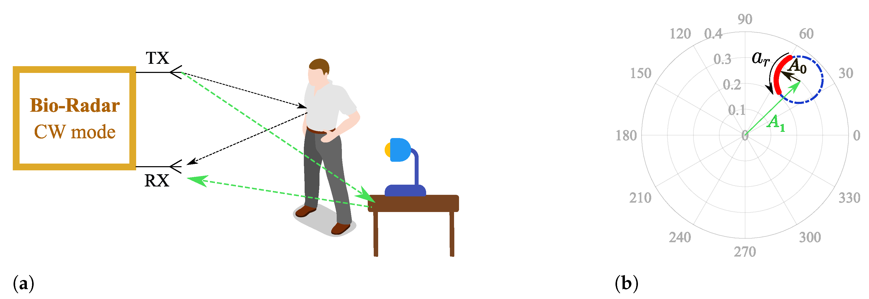
Figure 1a depicts the operation principle of a CW bio-radar. A sinusoidal signal is continuously transmitted towards the subject’s chest wall, and its reflection is received by the radar front-end. The chest wall moves periodically due to respiration and heart beating, changing the traveled path of the electromagnetic wave. Thus, these chest motions perform a phase modulation on the received signal, and vital signs can then be inferred after extracting this phase information.
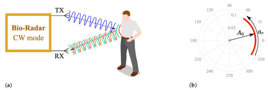
Figure 1.
CW bio-radar operating principle, where TX is the transmitting antenna and RX is the receiving antenna: (a) Illustration of an ideal scenario, (b) Resulting baseband signal in the complex plane for an ideal scenario.
Generally, Radio Frequency (RF) front-ends have quadrature receivers; hence, the baseband signals are processed as complex signals. Considering an ideal monitoring scenario, without any parasitic reflections, vital signs are perceived as an arc projected in the complex plane, as depicted in Figure 1b, where corresponds to the received signal amplitude and the phase variation proportional to the amplitude of the chest-wall motion. This arc disposition is related to the carrier frequency used [5]. With lower frequency carriers, the chest-wall displacement is lower in relation to the wavelength. On the other hand, if higher frequency carriers are used, the wavelength decreases and the chest-wall motion could be equivalent to several wavelengths. In this case, full circles are produced in the complex plane instead of arcs.
Considering that low frequency carriers are used, and knowing that ideal scenarios do not exist, the monitoring surrounding conditions must be accounted for when developing algorithms for vital signs extraction. Since CW radars are not able to measure the distance between the subject and the radar [7], the reflection from the chest cannot be isolated. Therefore, the received signal is a sum of the desired signal with other parasitic reflections that occur in stationary objects located within the monitoring scenario.
Parasitic reflections can be referred to as complex DC (CDC) offsets due to two main reasons: they increase the spectral component magnitude of 0 Hz, and they cause a misalignment of the phase signal in relation to the complex plane origin, as depicted in Figure 2, where corresponds to the parasitic component amplitude.

Figure 2.
Illustration of the effect of a static scenario in the complex plane: (a) Reflections schematics on the monitoring environment, (b) Equivalent projection of the received signal on the complex plane.
Thus, the CDC offsets must be removed to guarantee a proper phase demodulation for vital signs extraction, and several solutions have been reported in the literature.
The CDC offset removal can be performed through either software or hardware approaches. On the hardware side, antennas with high directivity can be advantageous, since they enable a focused steering on the desired area, enhancing the Signal-to-Noise Ratio (SNR) and reducing the parasitic reflections acquisition [10,11,12,13]. Nonetheless, the antennas’ size must increase in order to achieve directivity. While horn antennas are bulky [13], microstrip antenna arrays can be used as a more flat alternative. High directivity can be achieved using more microstrip patch elements, which not only increases the antenna size but also leads to the occurrence of side lobes able to equally acquire parasitic reflections. Furthermore, high directivity implies a perfect alignment between the subject and the antennas [13]. In this sense, the antenna design selection must respect a balanced trade-off and might not be sufficient to compensate the CDC offsets.
Thus, the CDC offsets compensation performed through signal processing might be more suitable for its simplicity and flexibility. For this latter case, the most direct solution would be the usage of a high-pass filter [14,15]. Although it would be a straightforward approach, filtering reduces the amplitude of vital signs [14] or could even cause distortion according to [16]. Moreover, filters can be used to remove the DC information related to the target’s position, which is necessary for the phase demodulation [16,17]. Some authors suggested a prior calibration, by measuring the CDC offsets of the environment without the target present in the room [18]. This solution is not practical, since it requires a calibration every time the system is used and is not effective if the monitoring scenario changes. In addition, other body parts can also be seen as static targets, and hence, they produce more parasitic reflections. Due to this fact, Park et al. [17] proposed another solution exclusively focused on the baseband arc shape. This solution is based on the arc center estimation and subsequent subtraction from the original signal. As a result, the arc position is re-established around the origin and the arctangent method [18] can be applied to recover the vital signs waveform. Currently, the center estimation approach is widely used in the literature [16,17,19,20,21,22], where circle or ellipse fitting methods are the most common.
Nonetheless, the estimation of the arc center can be compromised when signals have a low amplitude [20,23], especially if circle fitting methods are used. In fact, low-amplitude signals could be recurring for several reasons, such as multipath signal degradation, or when the vital signs are acquired in an alternate chest-wall position such as sideways rather than in front [24], or finally when the subject has lower chest-wall displacement. In [25], a relation is established between the sex of the subject and the amplitude of the chest motion. It is highlighted that women produce lower chest motions, since they also have a lower chest volume. This fact leads to received signals that are weaker but have useful information that can be extracted.
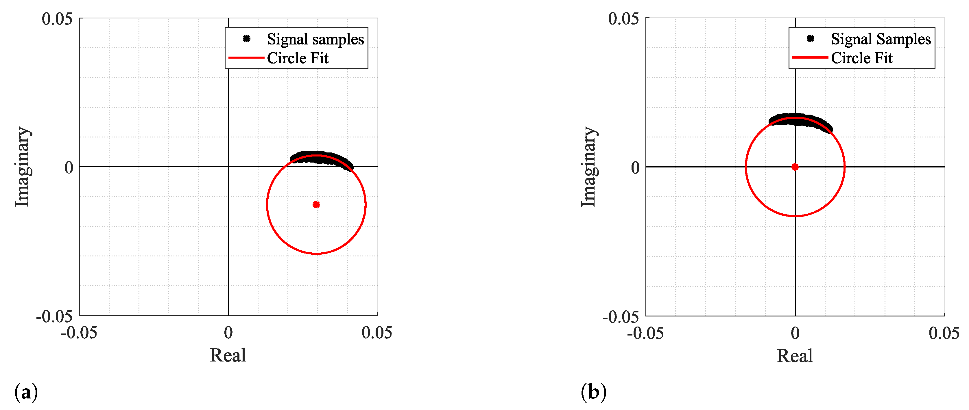
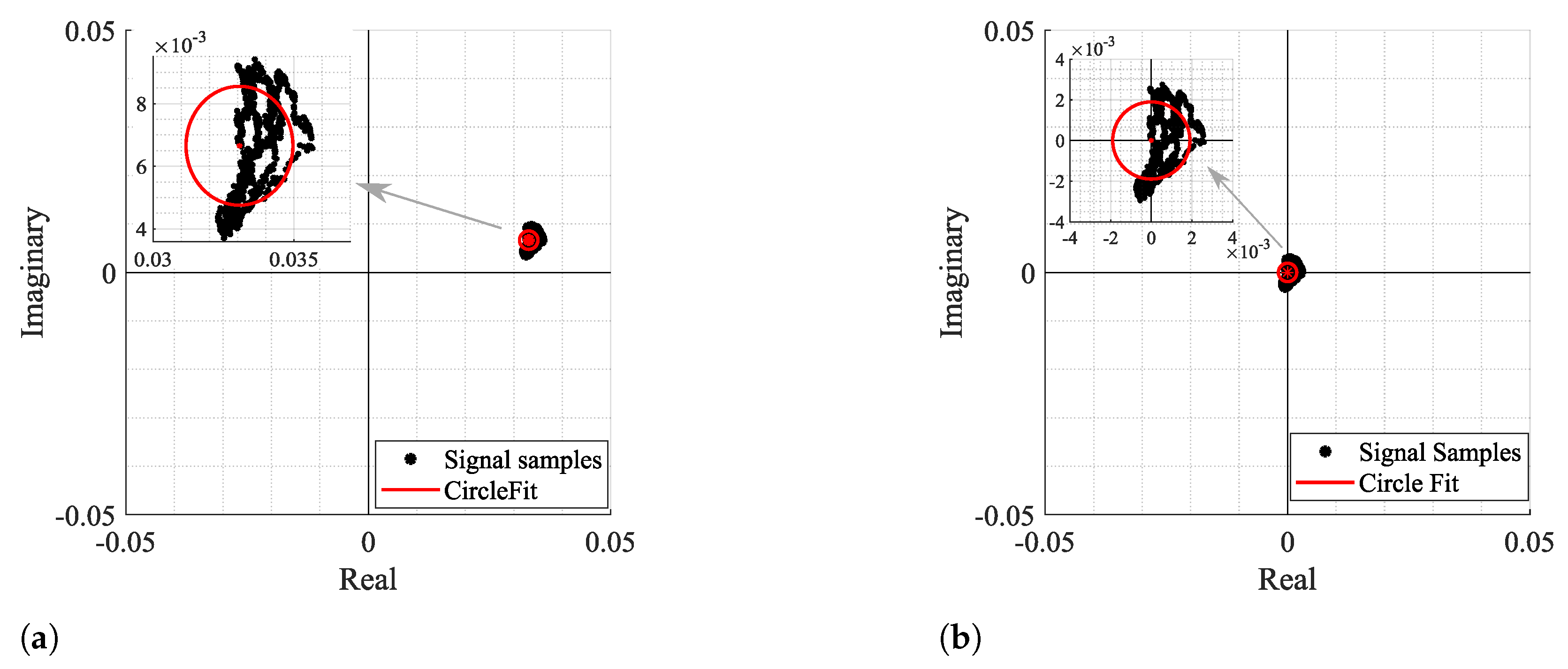
Figure 3 and Figure 4 show two examples of the possible signal arcs. Specifically, Figure 3 presents a well-defined arc corresponding to a received signal with high amplitude , and Figure 4 presents a case where is severely decreased, as well as its arc length . This consists of a weak signal case, since it has either low amplitude and the overall signal consists of several arcs dispersed rather than being concentrated in a defined area. In order to demonstrate the impact of the signal quality in the circle fitting performance, Figure 3 and Figure 4 also show the CDC estimation and removal results, using the Kasa method [26] as an example. In Figure 3, the center estimation can be easily inferred. On the other hand, in Figure 4, due to its lack of resolution, circle fitting algorithms consider that the overall sample cluster fits a circle, where its center is in between the radar samples, neglecting the supposed arc shape. Hence, the desired fitting is compromised and the center estimation is misleading. The case depicted in Figure 4a presents the result of a circle fitting with radius r close to 0, which in practice forces the arc to oscillate in the complex origin after the CDC offsets removal, later leading to incorrect arctangent results. Thus, for the CDC offset removal, the radar sample fitting must be performed correctly, by leaving a standard space between the arc and its estimated center; i.e., the arc radius r must be .

Figure 3.
Example of how fitting methods can provide an accurate center estimation: (a) Circle fitting result, (b) Arc disposition after removing the CDC offsets.
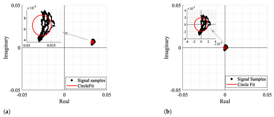
Figure 4.
Example of how fitting methods can provide an inaccurate center estimation, when there is a lack of data resolution, with its zoomed version on the right: (a) Circle fitting result, (b) Arc disposition after removing the CDC offsets.
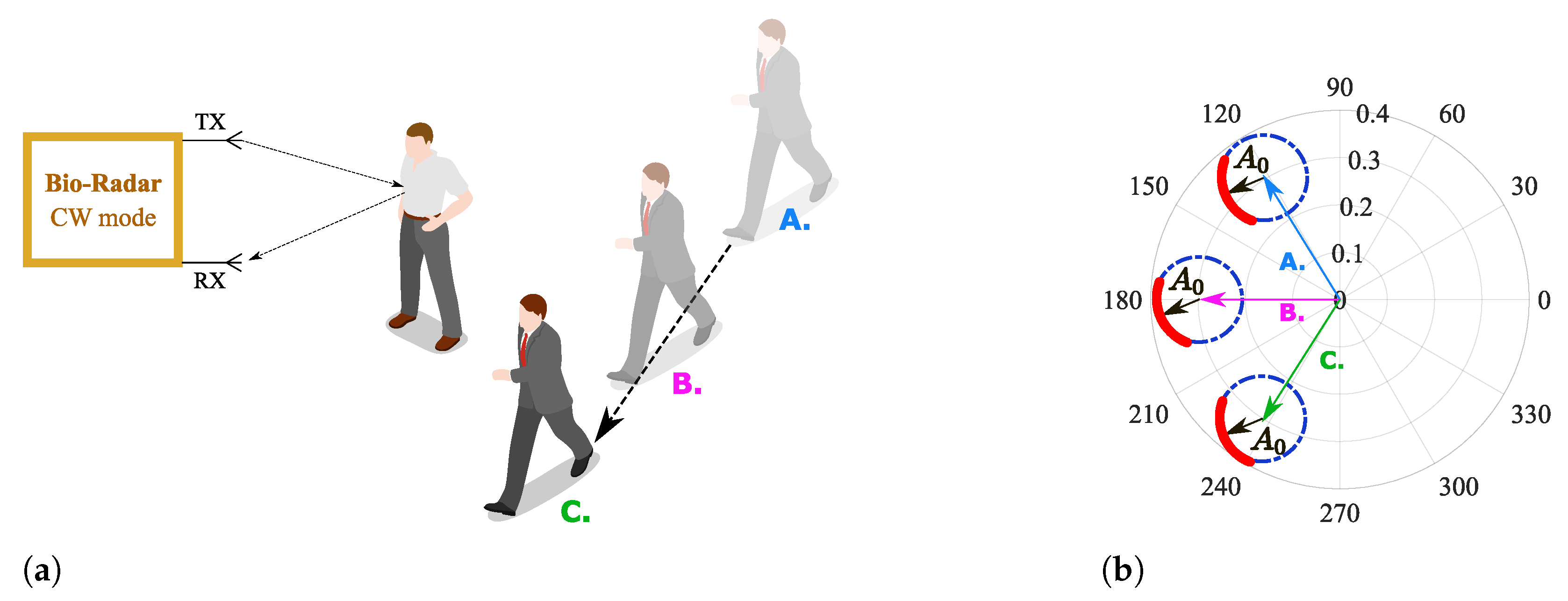
As in cases similar to or worse than the one presented in Figure 4, the formed arcs are not sufficient to estimate the corresponding fitting circle, and exploratory techniques can be implemented to search for more information in order to enhance the CDC offsets estimation. For instance, in [20,23], authors present approaches where multiarcs are induced to gather more CDC information by changing purposely the target’s distance in relation to the radar before starting the vital signs acquisition [20] or by tuning the local oscillators with different angles during the down-conversion of the received signal [23]. Nonetheless, real case scenarios present other challenges, which have a direct impact on the arc center estimation. Long-term monitoring applications should encompass slight motions from the subject when it is highly difficult to remain totally still during longer acquisition periods. Considering that these motions are not significant in the recovered signal, they can still uncover new objects located in the monitoring scenario, producing different CDC offset values. This situation can be worse when the monitoring scenario is not fully static. For instance, if other subjects move around in the same room, even out of the radar range, the parasitic reflections’ behavior changes accordingly, as figuratively depicted in Figure 5. Therefore, the arc center estimation must be performed over time, in order to encompass such changes smoothly [22]. This means that in offline signal processing, the CDC offsets removal cannot be performed using the full signal at once. The solutions presented in [20,23] were developed assuming that the scenario is fully static or that the signal’s characteristics, such as its amplitude, do not change over time. On the other hand, [22] uses a dynamic CDC offset cancellation with the goal to account for such environment changes. However, the authors only present signals from short acquisitions, with maximum 5 minutes duration. Moreover, the authors do not provide information regarding the algorithm’s effectiveness with low-amplitude signals.

Figure 5.
Illustration of the effect of a non-static scenario in the complex plane: (a) Reflection schematics on the monitoring environment, (b) Equivalent projection of the received signal on the complex plane.
In this paper, we propose a dynamic Digital Signal Processing (DSP) algorithm to remove the CDC offsets successfully over time, for every type of signal regardless of quality. This algorithm is robust to the impairments derived from the bio-radar handle in real contexts, where the monitoring environment might not be fully static and the subject’s signal characteristics might change over time. In this sense, signals from-long term acquisitions were used (with 25 minutes duration approximately). The algorithm is composed of the following features:
- It performs a robust removal of the CDC offsets coordinates, using a novel arc fitting algorithm, which is more effective even for low-amplitude signals;
- After removing the CDC offsets, the arc position is changed in the complex plane, to ease the vital signs’ extraction and rate computation;
- The full algorithm is implemented dynamically, through a windowing approach, in order to encompass wide environment changes;
- The dynamic implementation is smoothed, so the signal coherency and integrity are preserved.
The novel fitting method proposed herein was developed to be used in CW front-ends operating within the 5.8 GHz ISM band, where it can be assumed that the radar samples form an arc in the complex plane. Taking this fact as prior knowledge, and in order to avoid situations su h as the one depicted in Figure 4a, the algorithm is forced to search for an optimal arc center solution outside the radar samples. The optimization stage is not required, saving computational resources and enabling real time implementation.
After its development, the algorithm was tested using signals acquired in harsh conditions, in order to test its performance limits. Therefore, four case studies were considered, which included non-static acquisition environments, low-amplitude signals and portions of body motion. The algorithm effectiveness is directly related with the successful estimation of the arc center; therefore, its validation was conducted by comparing our novel fitting method with state-of-the-art approaches.
This paper is divided as follows: In Section 2 the proposed algorithm is described, with a special focus on the arc fitting algorithm and its dynamic implementation. Section 3 describes the set-up used and the evaluation metrics considered to test the algorithm performance and its limits. Results are discussed in Section 4, and Section 5 presents the algorithm’s behavior in cases where other body motions occur. Finally, conclusions are presented in Section 6.
2. Digital Signal Processing Algorithm
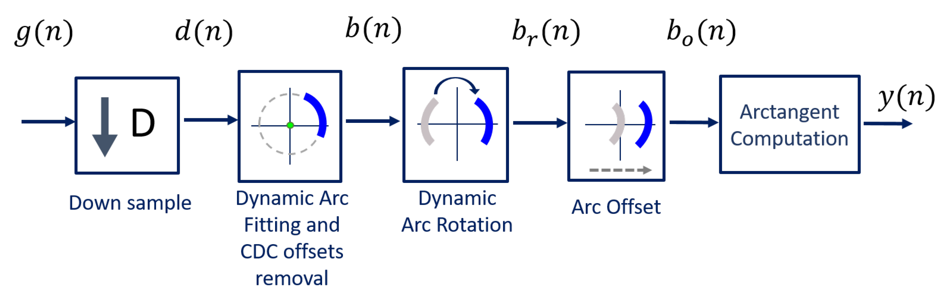
The algorithm was developed to be implemented with a CW radar operating at 5.8 GHz, considering the inherent issues that arise during its handling. The block diagram presented in Figure 6 sums up the algorithm working principle.
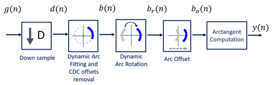
Figure 6.
DSP algorithm for extraction of vital signs.
Usually, signals are acquired by quadrature receivers in CW radars, with a high sampling rate due to front-end restrictions [27]. The front-end output consists of a complex baseband signal , which was acquired with a sampling rate equal to 100 kHz. Firstly, this signal is downsampled, since vital signs are low-pass signals. In our case, the decimated signal presents a sampling rate equal to 100 Hz, embracing both respiratory and heart signal characteristics.
Afterwards, the CDC offsets are estimated using our novel arc fitting method, and subsequently removed from the decimated signal , resulting in signal . In this stage, two concerns were noted:
- The CDC offsets should be correctly estimated, with ;
- The CDC changes should be tracked and accounted for, which can be accomplished by estimating the offset values dynamically over time through a windowing approach.
The novel arc fitting and its dynamic implementation are detailed in Section 2.1 and Section 2.2, respectively. After the CDC removal, the arcs can be located in any position in the complex plane. All arcs are rotated accordingly to oscillate around the 0 value, resulting in signal . One should note the advantages that the arc rotation stage provides: first, it prevents the oscillation around the value and avoids the wraps occurrence. Secondly, its rotation for a specific angle eases an automatic implementation. Furthermore, it also eases the computation of the vital signs rate. Since is a phase signal, the location of the arc in other quadrants would increase the magnitude of the spectral component in 0 Hz. After the rotation step, the average angle is approximately , which enables the automatic computation of the vital signs rate through the identification of the spectral component with higher magnitude. The arc rotation is also performed dynamically, and this procedure is also detailed in Section 2.2.
Then, and as one will see later, if the implementation of the algorithm fails to remove the CDC offsets successfully, there will be samples crossing the origin. In those cases, a small offset can be added to push them away, resulting in signal .
Finally, the vital signs information can be correctly extracted using the arctangent method [18], thus obtaining signal . In this case, we applied this method to complex signals, using the angle function from MATLAB.
2.1. Arc-Fitting Algorithm
In order to remove the CDC offsets in bio-radar signals, the literature usually presents fitting algorithms that aim to search for a circle that fits the radar complex samples, finding its radius and center coordinates, which are used afterwards to remove the CDC offsets. Least Squares Fitting (LSF) is a common example of this approach [28]. Moreover, in cases where the data are well distributed, the literature suggests that the Gauss–Newton method with the Levenberg–Marquardt correction (LM) is an LSF -robust solver, which is quite stable, reliable, and fast-converging [21,28]. It uses a cost function and identifies the possible solutions by finding the parameters that lead to minimization of the cost function [21]. For instance, in [22], a circle fitting method is implemented to remove the CDC offsets using a cost function minimization. The center coordinates are identified when the radius variance is minimized. Nonetheless, both LM and [22] methods require an optimization stage, which consumes an unknown process time to achieve the desired solutions. Additionally, algorithms based on LSF are sensitive to outliers [29] and hence might not be effective in cases where the data are noisy or lack in resolution, which is a common case in the bio-radar context, as demonstrated previously in Figure 4.
Other impairment of the circle-fitting methods usage for bio-radar CDC removal relies on the dependence of the circle radius as an optimization parameter. Badly formed arcs with low lengths and wide thicknesses can drive the algorithm to provide center solutions within the radar signal samples, as demonstrated in Figure 4. The algorithm is forced to search for a circle that fits all points, assigning the radius that enables this fitting. In these situations, the cost-function’s minimum zone is located within the radar data points, which correspond to the center of such circle. For instance, Figure 7 presents a case where the considered optimization starting point was the radar signal mean value, which was already located in a minimum zone. Under these circumstances, it was impossible to find a proper center point outside the data samples, even if the number of iterations is increased or the boundary conditions are wider.
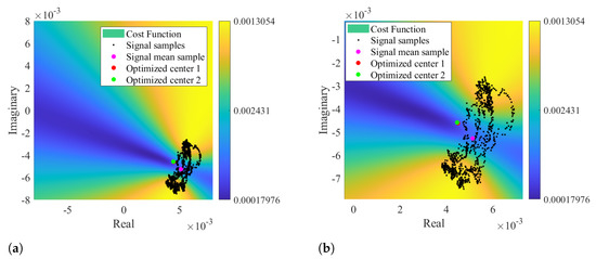
Figure 7.
Color map of the cost function result using signal mean value as optimization starting point: (a) Representation of the optimized solution, (b) Zoomed visualization of the optimized solution.
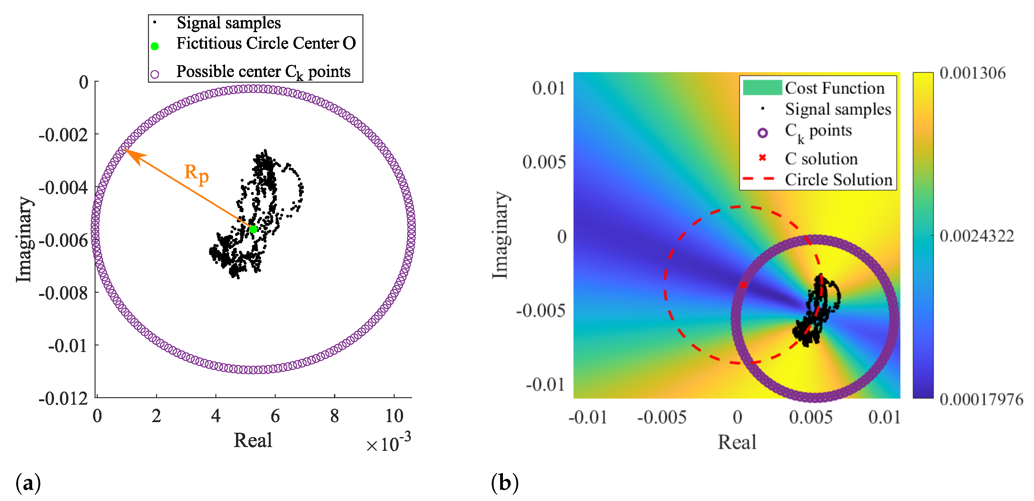
By taking as prior knowledge that the radar samples are disposed according to an arc rather than a circle, it is possible to set the searching zone already outside the signal samples, since the minimum zone extends on the arc’s forward area. In this sense, we developed a novel arc-fitting method that aims to determine the most appropriate center of the arc formed by the radar samples. This new method, from now on referred to as Optimized Cost (OC), is also based in a cost-function minimization. The searching area is limited to the arc sideways zones, avoiding the center solutions within the radar samples. For this purpose, a set of circularly distributed points were defined as possible arc center points, as depicted in Figure 8a.

Figure 8.
Illustration of the novel arc fitting method: (a) definition of the possible Ck solutions, (b) cost function result with the selected C solution.
Those points form a fictitious circle with radius , selected to push the estimation away from the radar samples. The radius is expressed by Equation (1):
where is an arbitrary scale factor, denotes the median value, P is the radar samples, and O is the center of such fictitious circle, given by Equation (2):
where is the median of the complex number P, performed separately in the real and imaginary parts of P, respectively. The scaling factor dictates how much larger the searching area should be, considering the arc length. In order to guarantee that the selected center C is not within the arc samples, the scaling factor should be . In the context of this work, the value was selected empirically, and it was used the same value for all signals.
The arc center solution C is obtained through the cost function minimization, calculated with each and given by Equation (3).
where is the considered k point, are the radar samples and r is the radius of the arc. In contrast to the aforementioned methods, r is not an optimization parameter, once it is subsequently estimated using the median computation on Equation (4):
Therefore, r depends on the solution, avoiding the tendency to provide solutions within the data points. The median operation was used in Equations (1), (2) and (4), as it is a robust estimator in case of outliers [29].
After obtaining the points and evaluating the function for each, the final C solution is the that allows to be minimum. Therefore, C can be written as (5):
Since the searching area is already limited outside the radar sample points, the solution is direct and does not require any optimization stage. This procedure is depicted Figure 8b, where the most suitable arc center is marked with a red cross.
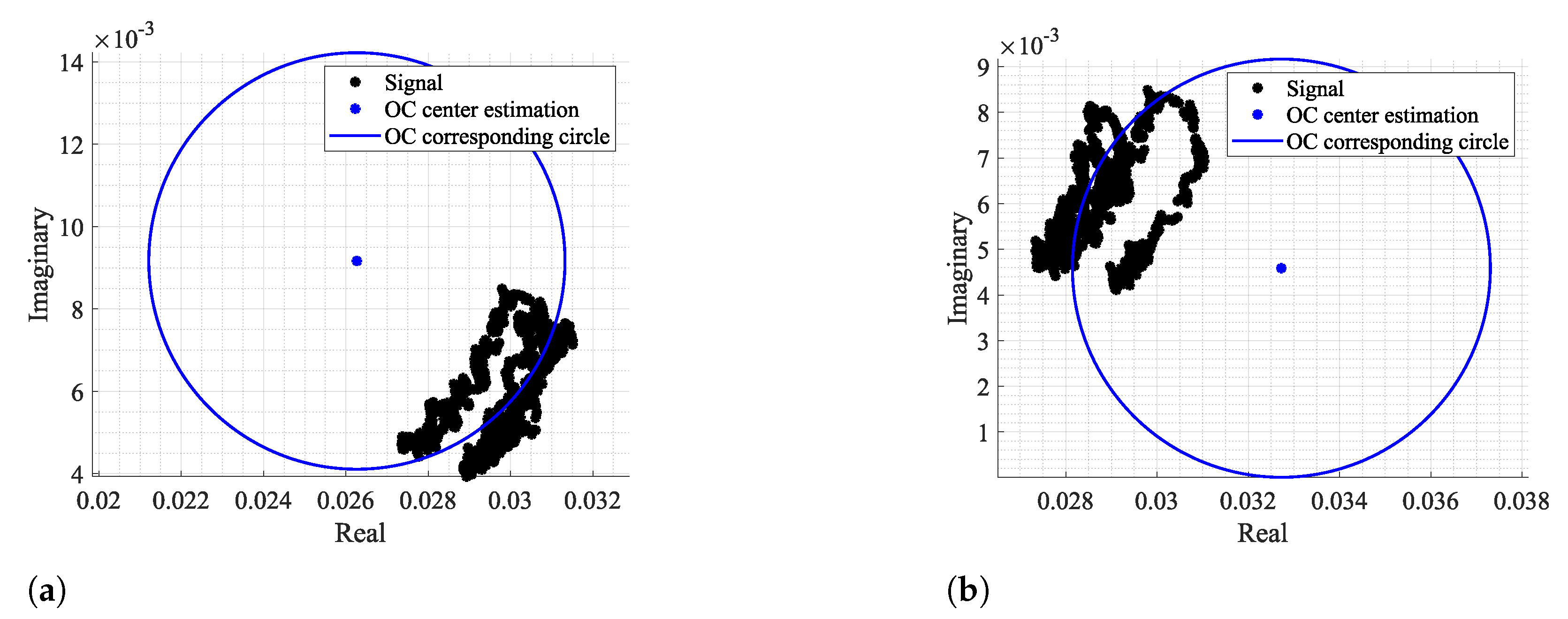
One should note that the OC algorithm presents three limitations. First of all, the S minimum zones can occur in both arc sides, i.e., inside and outside its concavity, as can be observed in Figure 8b with the location of the dark blue zones. The next sub-section explains the dynamic implementation of this algorithm to accommodate CDC changes over time. Such implementation requires the CDC estimation of overlapped windows in order to provide a progressive and coherent CDC estimation over time. When signals are especially weak, successive windows might present C solutions at opposite sides of the arc, as depicted in Figure 9, adding an undesired variability degree to the overall center estimation.

Figure 9.
Center estimations in opposite arc sides in consecutive windows, using as an example: (a) the window n° 74, (b) the window n° 75.
In order to avoid this issue, the distance between the current window center C and the last acceptable window center was included as a new cost in the cost function. Therefore, Equation (3) should be re-written as Equation (6):
where represents a weight and is the last acceptable center estimation. The center is selected and updated if it is located far from the radar samples P.
This new term reduces estimate transitions in successive windows by giving to a fair value, keeping in mind that lower values allow more transitions and higher values avoid necessary transitions, when the arc orientation changes. In this case, the term was set to 1.
The second limitation regards the vital signs’ amplitude, after performing the arctangent method. The searching area is set outside the radar sample points by giving a considerable value to the scale factor. This value must be selected while keeping in mind that it should always provide estimates outside the radar data samples. However, a special care should be given, since larger values push the arc away from the complex plane origin, reducing the angle variation range. Therefore, higher amplitude vital signs are obtained if the arc is located close to the origin, but its amplitude can slightly decrease if they are too distant. This also means that the final signal amplitude might not be the original one. The amplitude variation over the original signal can indicate changes in the subject’s psychophysiological state. Therefore, one should use the same for all signal windows in order to try to preserve the maximum possible eventual signal amplitude variations.
Finally, as mentioned previously, in order implement this algorithm, the radar samples must be disposed according to an arc, which is only valid when low-frequency carriers are being used. Higher carriers induce full circles instead of arcs, and in these cases, the traditional circle-fitting algorithms are indeed more appropriate.
2.2. Dynamic CDC Removal and Arc Position Adjustment
As seen previously, long-term monitoring periods could embrace CDC offset changes over time, not only due to any eventual subject body motion, but mostly due to changes in the scenario disposition during the monitoring period. Thus, the DSP algorithm should encompass such changes dynamically as their occur in order to preserve the arc information.
The CDC offsets can be removed and compensated over time by performing the arc fitting with a windowing approach, enabling an implementation for both offline signal processing (which is the case of this work) or in a real-time application (with the proper adjustments to maximize the algorithms’ performance).
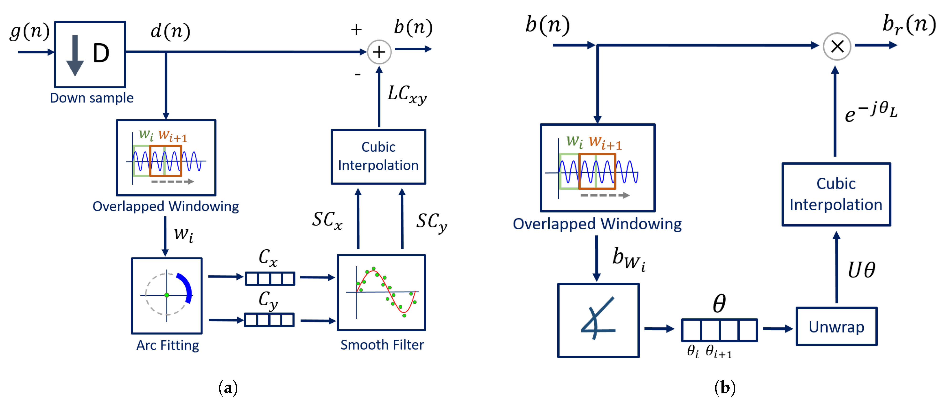
The implementation of the dynamic CDC removal is depicted in Figure 10a. The decimated signal is divided into windows with 1000 samples length and with overlap while moving forward. This window length was selected considering our sampling frequency (equal to 100 Hz after downsampling) and the possible respiratory rates across the population. Healthy subjects generally breathe at a rate around 0.2 Hz (12 breaths/min) [30], but it is also possible to reach lower values such as 0.1 Hz (6 breaths/min) [31]. Under these circumstances, 10 seconds is required to obtain a full arc, leading to a minimum of 1000 samples and thus always guaranteeing that a complete arc is obtained. The same approach was used in [22].
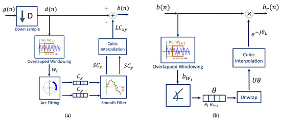
Figure 10.
DSP dynamical implementation: (a) Dynamic CDC removal, (b) Dynamic arc rotation.
The arc fitting method is applied to each window , and the center C coordinates are stored in two vectors, one for the real coordinates and other for the imaginary ones . As we will see later, our proposed method is relatively stable, when comparing with other well-known fitting methods. Nonetheless, after inspecting all signal windows, a smooth filter was applied to the each vector in order to prevent outliers. The selected smooth filter was a 1st-order Savitzky–Golay filter with a frame length equal to 31, resulting in smoothed vectors and . Then, the vectors are interpolated using the shape-preserving piecewise cubic interpolation, resulting in the vectors and , which form the complex number . The cubic interpolation was selected for providing a smooth interpolated vector and for having a good approximation behavior on the vector extremes [32]. Finally, the interpolated vector is subtracted from the decimated signal , resulting in signal (from Figure 6).
After removing the CDC component, the arc position in relation to the complex plane should be adjusted in order to avoid wraps that can occur when the arc is located between the second and the third quadrants, crossing the value. The CDC change over time also affects the arc orientation in relation to the origin. Therefore, this rotation step must also be implemented dynamically over time by dividing the signal in windows again. This procedure is depicted in Figure 10b. The goal is to rotate all window arcs until they oscillate around the angle. This is performed by computing, for each window, the necessary angle required to rotate the arc. This is accomplished using Equation (7):
where is the necessary angle to rotate the arc from window i. Similarly to the CDC offsets’ window estimations, an angle vector is created with all values. The vector is unwrapped and interpolated using the same interpolation used for the CDC offsets. Then, the full signal is evenly rotated by applying Equation (8), resulting in signal :
where is the full signal without CDC offsets and is the angle vector, unwrapped and interpolated.
After properly centering the arc around the origin, weaker signals might require an additional step. The implementation of Equation (6) in the arc-fitting stage decreases the number of estimation transitions, but does not solve them all. When there are transitions in successive iterations, it affects the overall estimation in that signal portion by considering the mean of those consecutive values, and the arc is pushed to the origin after the CDC offsets’ removal. In these cases, it is necessary to shift the arc position slightly away from the complex origin. For this purpose, a small offset can be added to the full complex signal, resulting in signal . This offset can also be computed automatically: when the final arc is centered in the origin, there are samples with a negative values on the real component. Therefore, the signal with an offset can be obtained by applying Equation (9):
where denotes the minimal value of the real component of signal.
3. Algorithm Testing
After the algorithm development, its limitations and performance were tested, considering real application scenarios. This section presents the set-up used to acquire the vital signs, the monitoring conditions, and the metrics considered for the efficiency evaluation.
3.1. Front-End Description
In order to acquire the subject’s vital signs, a bio-radar prototype was used operating in CW mode at 5.8 GHz and with 7 dBm as the transmitted power. The set-up was composed by an RF front-end, namely the USRP B210 board from Ettus ResearchTM [27]. The transmission and reception antennas were antenna arrays, with crossed circular polarization, to avoid the mutual coupling and to improve the path gain [33]. Both antennas have a gain equal to 12.2 dBi and half-power beamwidth of approximately. The subjects were seated in front of the antennas at a distance of half a meter.
Bio-radar signals were acquired using the GNU Radio Companion software, with a sampling frequency equal to 100 kHz. Then, the algorithms mentioned herein were applied offline using MATLAB software.
3.2. Evaluation Metrics Description
In order to test the proposed algorithm, the vital signs of three different subjects were acquired within approximately 25 min. Each subject represents a different case study with specific acquisition conditions, embracing both problems mentioned herein: the CDC offsets changing over time and the lack of arc resolution, which hampers the arc center estimation. Vital signs were acquired in two different monitoring scenarios and using subjects with different genders, in order to provide unequal chest-wall displacement amplitudes according to [25]. The considered case studies are described in Table 1, and the corresponding baseband signals can be observed in Figure 11.

Table 1.
Case studies description.
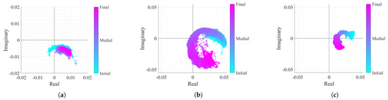
Figure 11.
Real/Imaginary plots of the considered case study baseband signals: (a) Case 1, (b) Case 2, (c) Case 3.
The first case signal, shown in Figure 11a, represents a reference case study, with a high displacement amplitude acquired in a static environment. In Figure 11a, it can be seen that the arc center rarely moved. Nonetheless, a slight displacement might be justified with eventual motions that the subject did, since it is difficult to remain completely still for such period of time. In the second case (Figure 11b), the CDC variation challenge is introduced. In this case, it is possible to observe that the arcs are changing their position over time. Finally, the last case study in Figure 11c represents the worst case scenario, where besides the CDC variation, the signal presents a lower amplitude derived from a lower chest-wall motion.
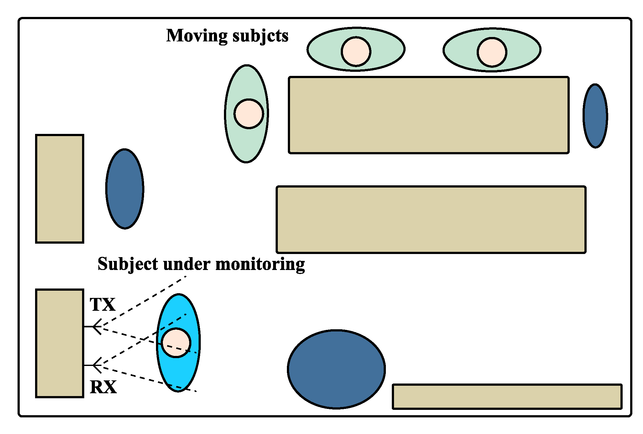
The scenario schematics used on these experiments is depicted in Figure 12. In order to induce the non-static scenario for cases 2 and 3, the vital signs were acquired in a room with other subjects inside, who moved slightly and sporadically. The moving subjects were located outside the antennas beam and hence did not interfere on the received signal directly. The static scenario used the same layout as the one shown in Figure 12, but without the additional moving subjects.

Figure 12.
Schematics of the monitoring scenario used for the experiment.
For all cases, the algorithm presented in Figure 6 was equally applied. Since the window length was equal to 1000 samples and signals were processed with a sampling rate equal to 100 Hz, more than 420 windows were analyzed per case study. The results presented in this work are mainly focused on the arc-fitting performance. The final aspect of each case study signal after the DSP algorithm implementation is also shown.
Regarding the arc-fitting analysis, this stage was performed using either the OC algorithm or any of the state-of-the-art circle fitting algorithms, namely the LM algorithm [28,34], the Kasa (KA) algorithm [26,34], the Taubin (TAU) algorithm [34,35]. The LM algorithm required an initial guess for the arc center coordinates C to further optimize. Hence, a fair comparison could be performed using as starting coordinates the estimation provided by OC.
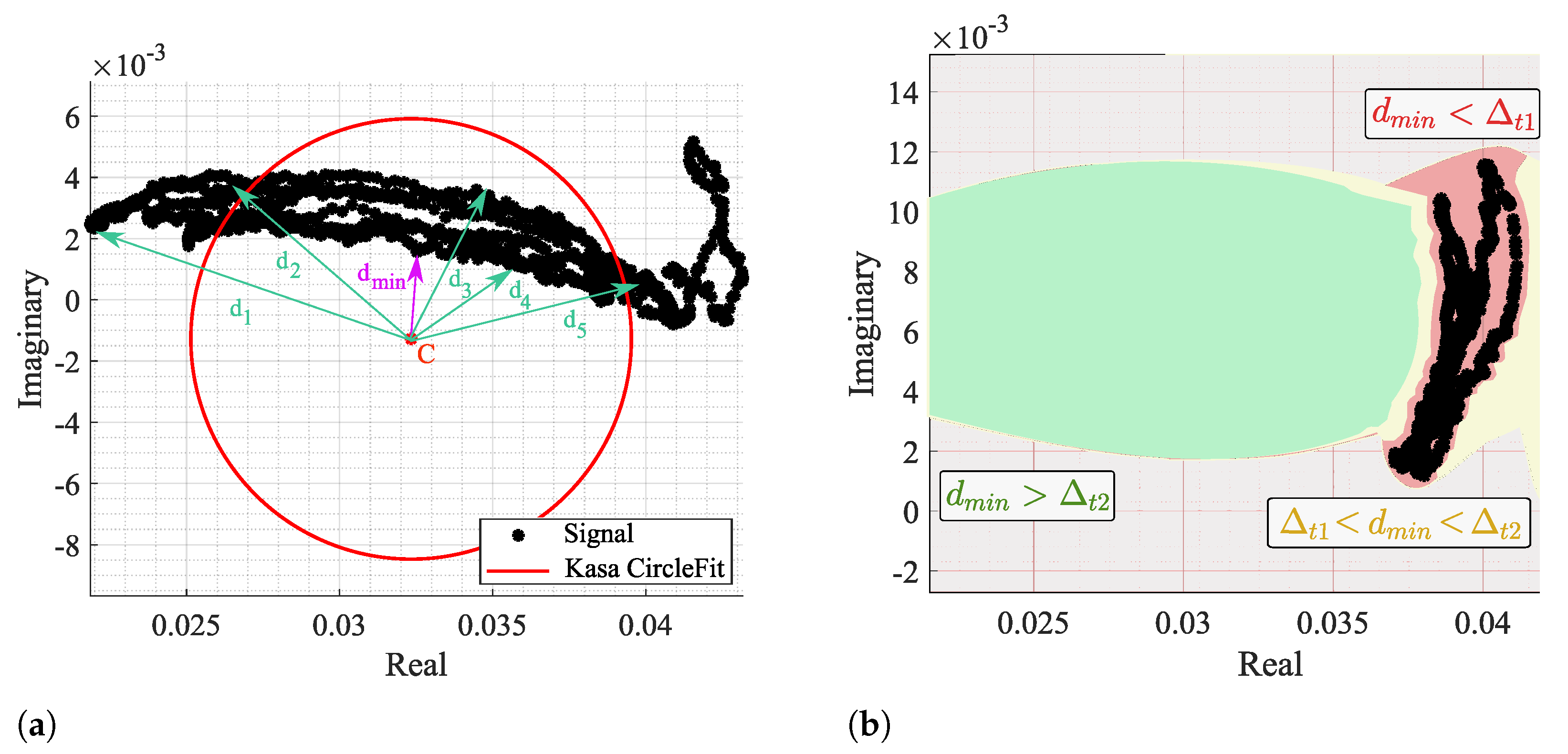
The fitting results were analyzed through the CDC offsets estimation for each algorithm in all signal windows, more specifically the location of C in relation to radar samples. It is considered a failure case when the C estimation is within the arc data samples, as previously presented in Figure 4. In order to identify a failure case, the distance between C and all signal samples was computed for all windows, as shown in Figure 13a.

Figure 13.
Identification of a failure case: (a) Illustration of the distance computation and identification, (b) Color map of the defined thresholds—red zone is defined when , yellow zone is defined when , and the green zone is defined when .
Then, the minimum distances of all windows were analyzed, and two thresholds were defined: and , as depicted in Figure 13b. When , it means that C is located in the red zone, within the arc data samples, and this is a clear failure case. On the other hand, if , it means that C is out of the arc samples yet too close, being in the yellow zone. The cases above the threshold are in the green zone and can be considered admissible, since it already allows the correct angle estimation and further arc rotation. However, the cases near this limit also require the offset addition shown in Figure 6.
When the fitting is applied dynamically, the CDC offsets estimate must not vary significantly, so as to guarantee a successful interpolation and smooth DC removal in the overall signal. Therefore, it is also crucial that the selected fitting algorithm provides stable estimates among the different signal windows.
In sum, the considered metrics to evaluate the arc fitting performance are:
- The behavior of estimations over time, obtained through the first difference of consecutive C estimations - .
- The standard deviation of consecutive C estimations (), where is computed in the complex form;
- The percentage of failure cases () for each case study;
- The percentage of cases that can be critical to the algorithms performance () for each case study;
- The average run time that each algorithm takes to provide a windowed estimation.
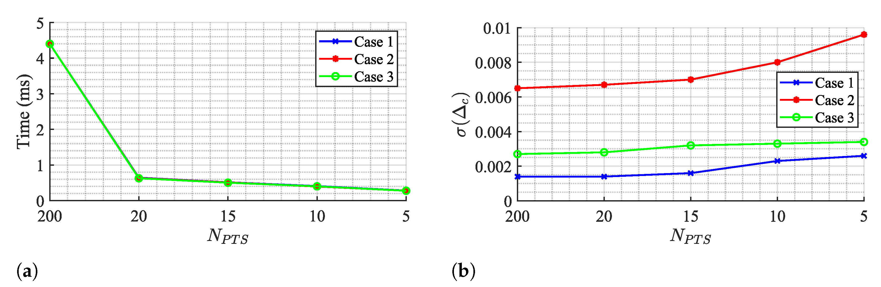
Although the OC algorithm do not require an optimization stage, the number of points used in the fictitious circle (from now on referred as ) have an impact on the computational time. For starters, the fictitious circle has been a total of 200 points, which respects a balanced trade-off between resolution and time consumption. Results are also presented with a lower number of points, so as to verify the impact in computational time and in the algorithm performance.
Additionally, and since the algorithm presented herein applies a Golay filter on the vector containing the CDC estimations (before interpolating it), the smoothed vector version is the one used for the removal of CDC offsets rather than the original estimation provided directly by the OC algorithm. This means that the method can actually fail and the arc can reach the complex origin, which is undesired. Therefore, the performance evaluation also includes the number of failure cases after removing the CDC offsets using the OC method. For this purpose, the signal was again divided in windows and the same metrics are used, where is now related to the minimal distance between the arc samples and the complex origin, refers to the estimation variation after applying the Golay filter, and the run time now regards to the CDC estimation and removal using the OC method. This evaluation was only performed for 200 points, which represents the most optimistic case.
4. Results and Discussion
In general, different estimations of the C coordinates were obtained by the different algorithms. Case study 1 was the one that provided more similar results, and case study 3 represented a limit case, where all algorithms presented a worse performance.
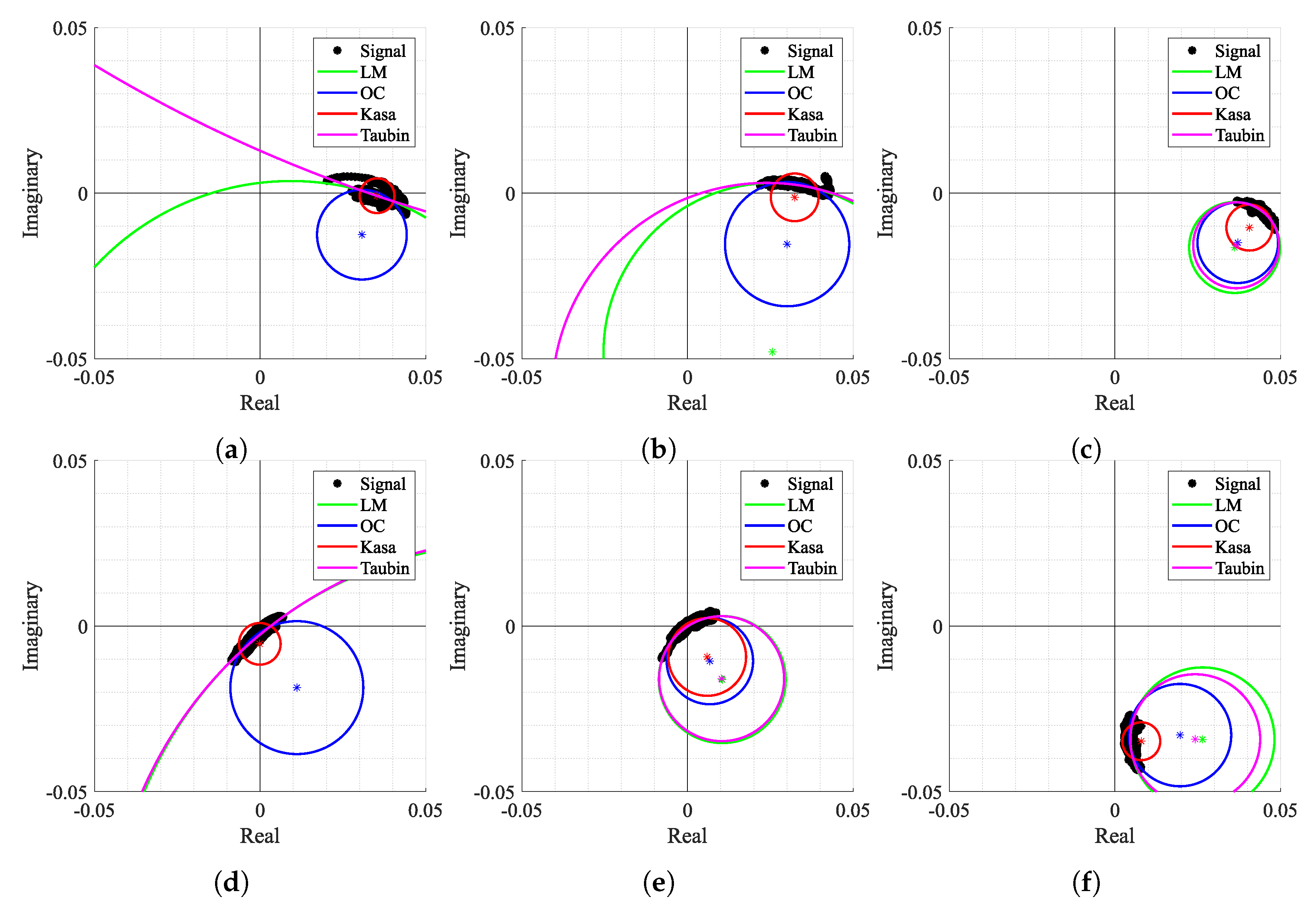
Since case study 2 includes a wide variation of the CDC offsets over time, but with a high chest-wall motion amplitude, it was possible to observe the most common estimation behaviors for all the tested algorithms. Figure 14 shows some examples of the estimation results throughout the signal, using the crescent order of window number. The first aspect that should be noticed is the arc position over the complex plane and its orientation. If signals were obtained in a static environment, the arc would barely move and would keep the same orientation over time. In this case, the contrary was observed as expected, since the motion of the moving subjects induce CDC changes. This arc position variation, along the windows, indicates the urge to perform both arc fitting and arc rotation dynamically.
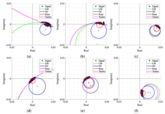
Figure 14.
Circle fitting result over time for case 2: (a) Window n° 2, (b) Window n° 4, (c) Window n° 35, (d) Window n° 318, (e) Window n° 327, (f) Window n° 413.
Secondly, Figure 14 also shows how some algorithms provided discrepant estimates for C coordinates. For instance, in Figure 14a,b,d, the LM and TAU algorithms provided estimations out of the arc range, which were seen as outliers. This fact also contributed to an increase in variability of the provided solutions over time. Moreover, in Figure 14a,d,f, the KA algorithm failed since its estimation lay within the arc samples. On the other hand, Figure 14c,e present some cases where all algorithms provided approximate estimations without any failure. It is also important to notice that the OC algorithm presented a stable estimation for all the aforementioned examples without any failure cases.
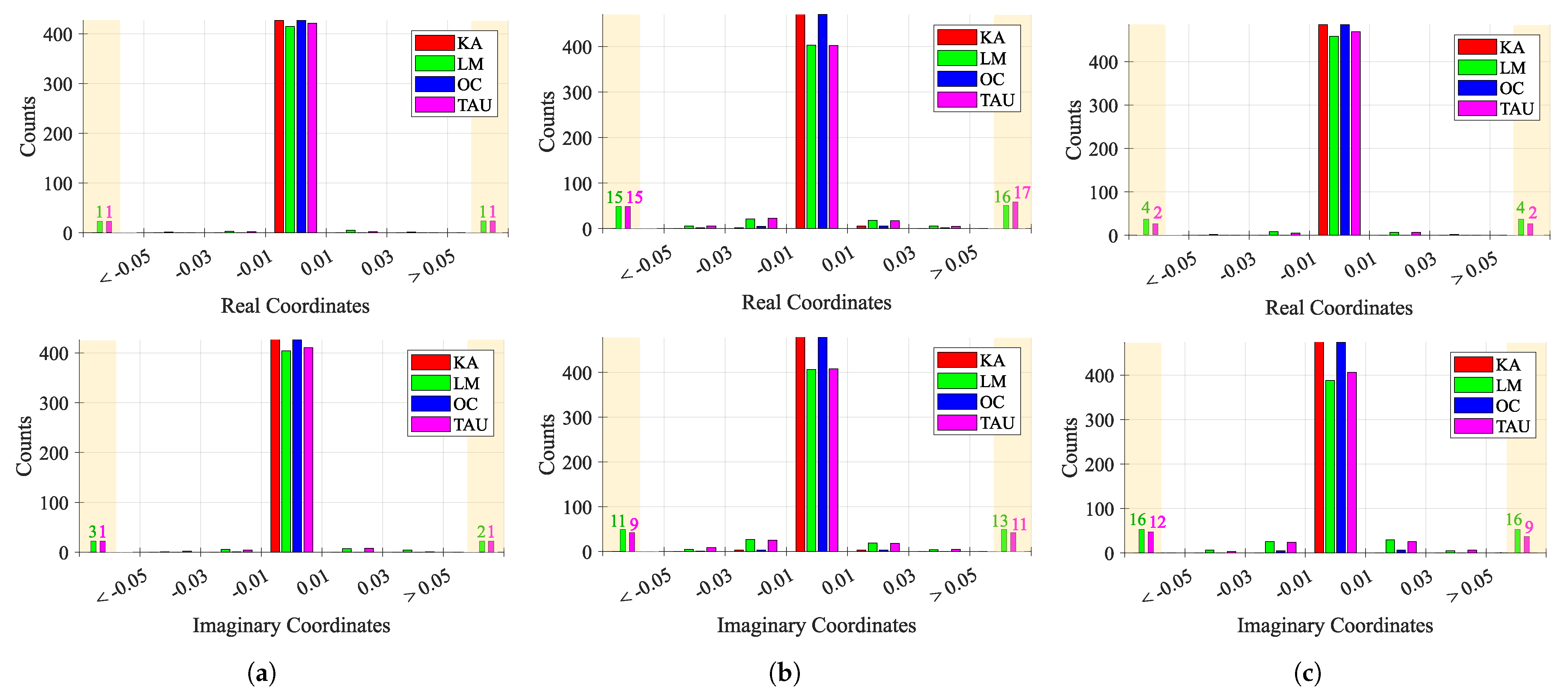
Figure 15 shows the behavior of consecutive estimations over time, for each case study. Considering that a perfect case would be one that presents more values near 0, which means that the consecutive estimations are the same, the first case study presented the lowest variation among all case studies, as expected. However, while KA and OC presented a stable estimation over time, LM and TAU algorithms provided few outlier estimations. The second and third case studies presented an increased variability, justified with the induced CDC change over time. In these cases, the estimations must track the CDC change over time, which justifies the overall variability. Once again, KA and OC were the more stable algorithms, when compared with LM and TAU, whose behavior worsened, showing a higher number of outliers greater than 0.05 and less than −0.05, respectively.
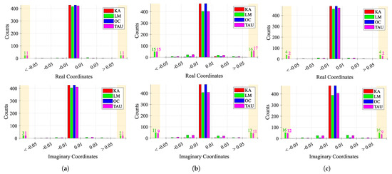
Figure 15.
Histogram of the behavior of consecutive estimations ΔC over time: (a) Case 1, (b) Case 2, (c) Case 3.
The overall fitting algorithms performance results are presented in Table 2, Table 3 and Table 4, for each case study, respectively. These tables contain the results relative to the estimations of the CDC offsets for all methods. Additionally, the final results of the arc location in relation to the complex origin are presented for the OC method.
Table 2.
Fitting results for case study 1.
Table 3.
Fitting results for case study 2.
Table 4.
Fitting results for case study 3.
Starting with the evaluation of the CDC offset estimations, for the first case study, all algorithms present a low percentage of failure cases. This was expected, since the first case is related to a chest motion with higher amplitude, acquired in a static environment. However, the KA method presents the worst performance, with of failure cases. On the other hand, the LM and TAU methods presented a higher estimation variation, with the highest value of . The OC algorithm is the one with the best performance, not only because it does not present any failure or any case within the critical limit, but also because it provided more stable results among all the signal windows. Regarding the run time, the KA and TAU are quicker, and this can be justified by the fact that they do not require any optimization stage (as the LM case), nor do they use a high number of points to search the solution (as the OC method), using in contrast algebraic computations for that purpose [26,35]. Nonetheless, if a lower number of fictitious circle points is used in the OC method, the run time of the OC method decreases considerably, and the algorithm performance is barely affected, as can be seen by the estimation variation and the same number of failure cases obtained.
For the second case study, it is possible to infer that the overall CDC offsets varied, since all values increased. One should note the sudden increase in for the LM method. This happened due to some outliers provided by the method, causing this high variation. The number of failure and critical cases barely changed for all methods, which might be related with the arc length of this signal. Once again, the OC method stands out with the best performance; however the number of critical cases increased slightly, if few circle points are considered.
Finally, the third case study served as a limit test. In general, a higher percentage of failure cases was observed for all methods due to the severe decrease on the arc length, excepting the OC method. The OC method kept a high performance, since we are searching outside the data points, rather than the other methods, which search for a fitting circle considering all data points. Thus, the KA presented the worst performance, with of failure cases and of critical cases. The remain algorithms, presented failure percentages above . The OC algorithm presented the same performance observed for the second case study, with 0 failure cases and only 0.2% of critical cases, regardless of the number of circle points used.
In fact, it can be seen from the results in Table 2, Table 3 and Table 4 that the impact of the number of circle points on the OC algorithm performance is weak, since parameter barely moved. Figure 16 shows the OC algorithm performance if points are even lower, by evaluating the run time and the , respectively.
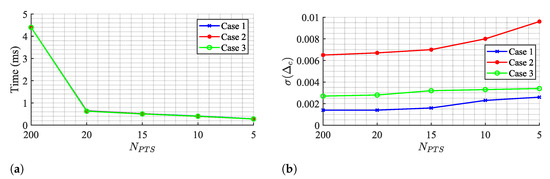
Figure 16.
OC algorithm performance for few Ck points: (a) Run time, (b) Estimation variability .
The run time decreases if the number of points is reduced, achieving a minimum value of 0.28 ms for a total of 5 points. However, this value is still above the TAU and KA algorithms and it comes with a cost of increasing estimation variability. Therefore, the selection of 20 points seems to respect a balanced trade-off between estimation stabilization over time and a decreased run time as possible.
Considering now the performance of the CDC offset removal using the OC method, a smoothed version of all the window estimations is used. This could lead to arcs ending close to the complex origin anyway, even if the initial estimation pushed it away. This was only observed in case 3, with of failed cases and of critical cases. Cases 1 and 2 remained with a high rate of success, presenting no failed cases after the CDC removal. On the other hand, the smoothing filter application highly decreased the estimation variability, as can be seen on the parameter for all cases. Finally, the implementation of the algorithm proposed herein, namely the CDC estimation using windowing, the smooth filter application, interpolation, and CDC removal takes approximately 2 s, regardless of the case study.
After removing the CDC offsets with the OC method and adjusting the arc position dynamically, all case studies should present equally optimal conditions for performing the arctangent demodulation. The only expected difference lies in the arcs amplitude, as can be seen in Figure 17.
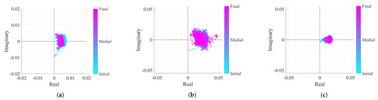
Figure 17.
Real/Imaginary plots of the considered case study signals after the DSP algorithm implementation: (a) Case 1, (b) Case 2, (c) Case 3.
5. Impact of the Body Motion on the Algorithm Performance
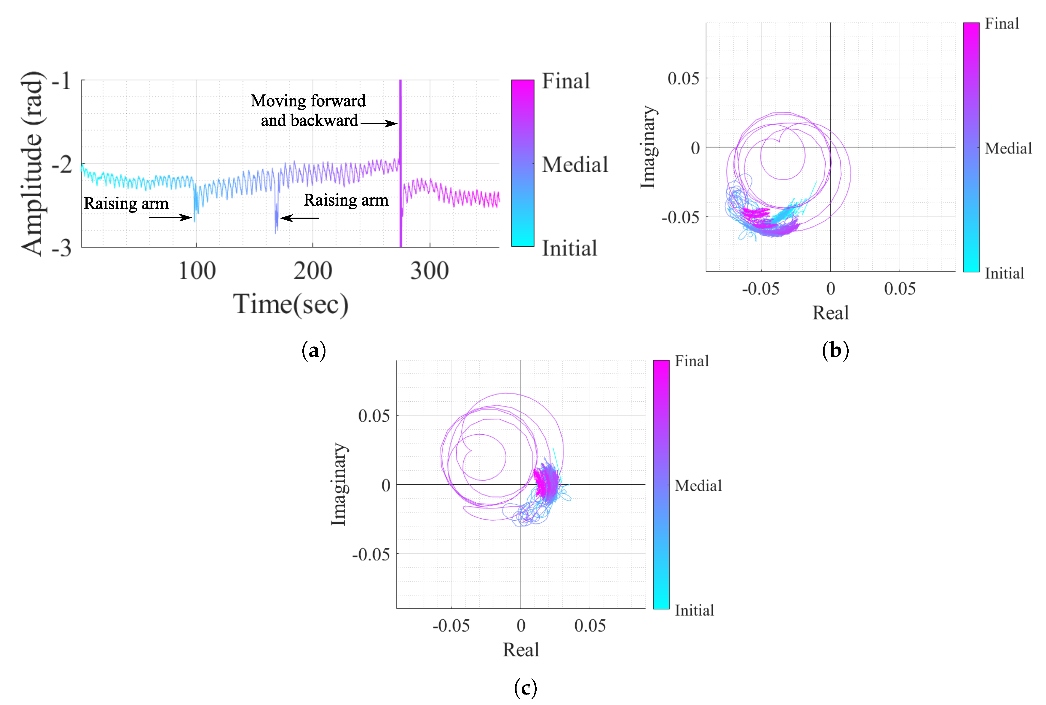
As mentioned previously, the OC method is more suitable for the acquired signals perceived as arcs in the complex plane. However, real case scenarios might contain signal portions with wide arcs or even full circles if the subject under monitoring moves their body during the monitoring period. In order to verify the performance of the algorithm proposed herein under conditions of random body motion, an additional case study was considered. The vital signs of a subject were acquired over 6 minutes, and the subject was asked to perform three specific motions: raising the arm and touching the head, raising the arm and touching the chest, and moving forward and backward in relation to the radar. Figure 18 shows the resulting signal in both time domain and the equivalent projection in the complex plane, before and after the implementation of the proposed algorithm.
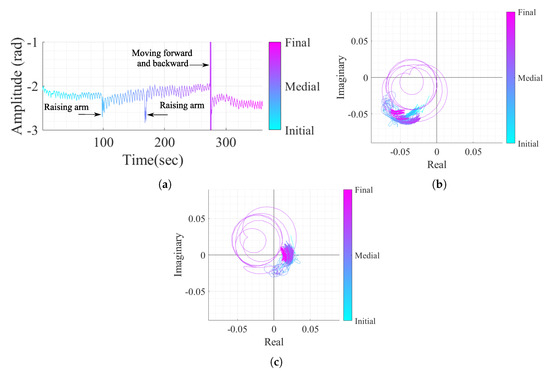
Figure 18.
Case study 4 containing vital signs with body motion: (a) Time domain signal with CDC offsets, (b) Real/Imaginary plots with CDC offsets, (c) Real/Imaginary plots after the DSP algorithm (without the CDC offsets).
By comparing Figure 18b,c, it is possible to verify that the algorithm is robust to sudden and sporadic motions, even if they present full circles in the complex plane. The algorithm was able to remove the CDC offsets successfully, regardless the presence of high amplitude motion and this fact can be justified by three features of the algorithm. Firstly, the usage of overlapped windows can address the motions smoothly by separating the motion into different windows. Secondly, the additional cost applied in the OC method (referred to in Equation (6)) is used to prevent estimation transitions and is also useful when motions occur, because the estimated CDC offsets stay in the same zone. Finally, the Golay filtering usage over the windows estimations before the interpolation also helped with the attenuation of eventual outlier estimations.
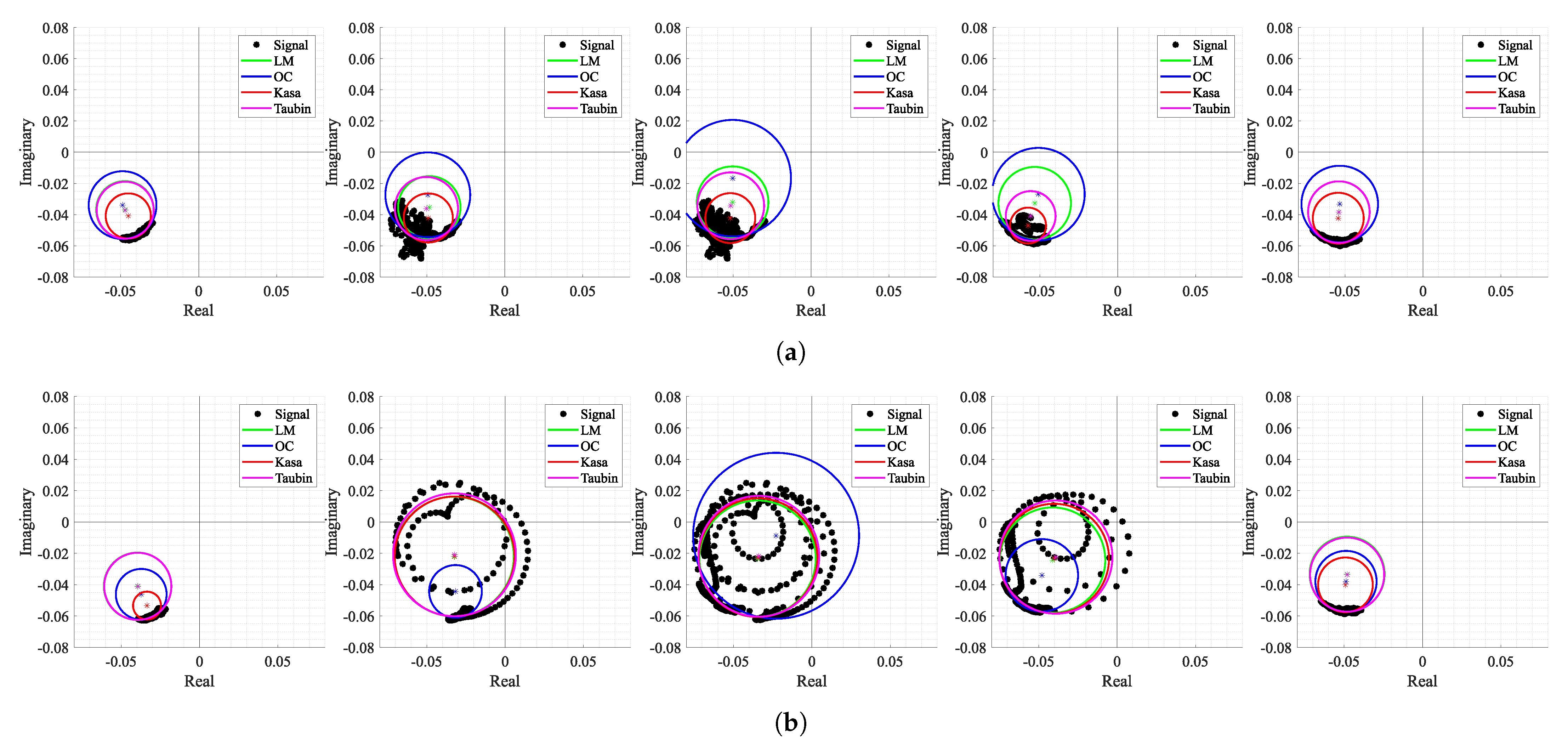
Figure 19 shows the corresponding shapes of arcs when the motions occurred and how all the tested algorithms behave under these circumstances. The first aspect that can be highlighted is the fact that not all types of motion generate full circles in the complex plane. For instance, raising the arm in front of the radar (see Figure 19a) generated a cluster of dispersed samples around what was supposed to be the arc. In this case, the OC method searches for a solution out of those samples, which is often close to the one obtained in the previous window. On the other hand, moving towards and backwards from the radar (see Figure 19b) generates complete circles, since the motion amplitude is equivalent to more than one wavelength, and the OC method kept the same behavior. Regarding the remaining algorithms, the LM was the most stable in the cases of both motions and the KA failed in the arm motion due to the wide cluster shape. As expected, both KA and LM algorithms seemed to provide accurate estimations of the exact values of CDC offsets when applied to full circles. Thus, the potential of the algorithm proposed herein might be enhanced if combined with the usage of traditional circle fitting methods, when a motion is detected. The motion of other body parts, which have been mostly seen as interference in bio-radar signals until now, can be used as additional information to accurately estimate the CDC offsets in parallel while monitoring vital signs, as previously proven in [36].
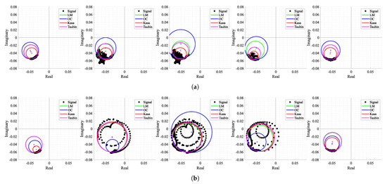
Figure 19.
Circle fitting result over time for case 4: (a) Windows 18 to 22 containing the motion of an arm raising up to the head, (b) Windows 53 to 57 containing the motion of the body moving forward and backward with respect to the radar.
6. Conclusions
In this work, a DSP algorithm is proposed to accurately recover the vital signs from a baseband bio-radar signal. This algorithm is robust enough to encompass two issues that arise when operating bio-radar systems in real applications: the CDC offsets change over time, when the monitoring scenario is not fully static, and the lack of arc resolution due to low-amplitude chest-wall motion.
For this purpose, the OC method was developed as an arc fitting algorithm and iapplied dynamically through a windowing approach. This method is based on a cost-function minimization that only depends on the arc center estimation. Circle-fitting algorithms presented in the literature, such as as the LM or KA methods, consider the circle radius as another variable in the minimization process. Furthermore, algorithms based on LSF optimization are highly sensitive to outliers, leading to center estimations within the signal samples. Herein, the OC method starts searching for a suitable solution outside the data points and is demonstrated to be robust in signals with low resolution.
Different fitting algorithms were tested using three case studies, where one served as a limit test embracing both issues aforementioned. The CDC component from a total of 1400 windows was analyzed using the OC algorithm as the proposed method and the LM, the KA and the TAU algorithms for comparison purposes. The proposed method did not present any cases of failure among all windows and presented only of cases in a critical situation. These results could be achieved using a lower number of searching points, reducing the run time. Additionally, it provides stable estimations over the full signal, as demonstrated by the standard deviation of the estimated CDC offsets. The remain methods present higher variability and a higher number of failure cases.
Nonetheless, the smoothed filter applied to the OC estimations led to nearly of failure cases after removing the CDC offsets, which resulted in some signal portions oscillating in the complex origin. The OC method also presented another limitation that requires a careful verification and eventual solution. Since the algorithm forces the arc center to be at a specific distance from the arc samples, the final signal amplitude can be altered from the original one. Further inspection on this issue is required, in order to verify if the method has any influence on the subject’s final breathing pattern by changing it in comparison with the original one.
After the CDC offsets removal, a dynamic arc rotation was performed to force the arcs to oscillate around the . This arc rotation presented several advantages, since it is thus possible to avoid the occurrence of wraps and enables easily computing the signals’ rate. Although the DSP algorithm was implemented and tested using offline signals, its flow allows a real-time implementation, taking a run time of 2 s to process full 25 min signals.
The effectiveness of the OC method in conditions of body motion was also tested, and it was successful in the case of sudden and sporadic motions. However, a more detailed study is required to understand the algorithm’s limits in terms of body motion duration and body motion types. As future work, we suggest exploring solutions that combine the DSP algorithm proposed herein with the usage of traditional circle-fitting methods, such as the KA one, when random body motion is detected. For that purpose, body motion should be classified into different levels according to amplitude and duration, and thus it should accordingly be decided which fitting method is more suitable.
Author Contributions
Conceptualization, D.A., C.G.; methodology, D.A., C.G.; software, D.A., C.G.; validation, C.G., D.A., J.V., P.P.; formal analysis, C.G.; investigation, C.G., D.A., J.V., P.P.; data curation, C.G.; writing—original draft preparation, C.G.; writing—review and editing, C.G., D.A., J.V., P.P.; supervision, D.A., J.V., P.P.; funding acquisition, C.G., D.A., J.V., P.P. All authors have read and agreed to the published version of the manuscript.
Funding
This work is funded by the Fundação para a Ciência e Tecnologia (FCT) through Fundo Social Europeu (FSE) and by Programa Operacional Regional do Centro under the PhD grant SFRH/BD/139847/2018, and under the project UIDB/05583/2020. Furthermore, we would like to thank the Research Centre in Digital Services (CISeD) and the Polytechnic of Viseu for their support.
Institutional Review Board Statement
Not applicable.
Informed Consent Statement
Informed consent was obtained from all subjects involved in the study.
Data Availability Statement
The data presented in this study are available on request from the corresponding author.
Conflicts of Interest
The authors declare no conflict of interest. The funders had no role in the design of the study; in the collection, analyses, or interpretation of data; in the writing of the manuscript; or in the decision to publish the results.
Abbreviations
The following abbreviations are used in this manuscript:
| CDC | Complex DC |
| CW | Continuous-Wave |
| DSP | Digital Signal Processing |
| FMCW | Frequency-Modulated Continuous-Wave |
| ISM | Industrial, Scientific and Medical |
| KA | Kasa |
| LM | Levenberg–Marquardt |
| LSF | Least Squares Fitting |
| OC | Optimized Cost |
| RF | Radio Frequency |
| SNR | Signal-to-Noise Ratio |
| TAU | Taubin |
| UWB | Ultrawide band |
References
- Lin, J. Non-invasive microwave measurement of respiration. Proc. IEEE 1975, 63, 1530. [Google Scholar] [CrossRef]
- Lin, J.; Dawe, E.; Majcherek, J. A non-invasive microwave apnea detector. In Proceedings of the San Diego Biomedical Symposium; Academic Press: New York, NY, USA, 1977; Volume 16, p. 441. [Google Scholar]
- Lin, J.; Kiernicki, J.; Kiernicki, M.; Wollschlaeger, P. Microwave apexcardiography. IEEE Trans. Microw. Theory Tech. 1979, 27, 618–620. [Google Scholar] [CrossRef]
- Chan, K.; Lin, J. Microprocessor-based cardiopulmonary rate monitor. Med. Biol. Eng. Comput. 1987, 25, 41–44. [Google Scholar] [CrossRef] [PubMed]
- Li, C.; Xiao, Y.; Lin, J. Design guidelines for radio frequency non-contact vital sign detection. In Proceedings of the 29th Annual International Conference of the IEEE Engineering in Medicine and Biology Society, Lyon, France, 23–26 August 2007; pp. 1651–1654. [Google Scholar]
- Gouveia, C.; Loss, C.; Pinho, P.; Vieira, J. Different Antenna Designs for Non-Contact Vital Signs Measurement: A Review. Electronics 2019, 8, 1294. [Google Scholar] [CrossRef] [Green Version]
- Pisa, S.; Pittella, E.; Piuzzi, E. A survey of radar systems for medical applications. IEEE Aerosp. Electron. Syst. Mag. 2016, 31, 64–81. [Google Scholar] [CrossRef]
- Union, I.T. Radio Regulations—Edition of 2016. Available online: https://itu.tind.io/record/25397?ln=en (accessed on 10 September 2021).
- Wang, G.; Munoz-Ferreras, J.M.; Gu, C.; Li, C.; Gomez-Garcia, R. Application of linear-frequency-modulated continuous-wave (LFMCW) radars for tracking of vital signs. IEEE Trans. Microw. Theory Tech. 2014, 62, 1387–1399. [Google Scholar] [CrossRef]
- Das, V.; Boothby, A.; Hwang, R.; Nguyen, T.; Lopez, J.; Lie, D. Antenna evaluation of a non-contact vital signs sensor for continuous heart and respiration rate monitoring. In Proceedings of the IEEE Topical Conference on Biomedical Wireless Technologies, Networks, and Sensing Systems (BioWireleSS), Santa Clara, CA, USA, 15–18 January 2012; pp. 13–16. [Google Scholar]
- Hsu, T.; Tseng, A. Compact 24 GHz Doppler Radar Module for Non-Contact Human Vital Sign Detection. In Proceedings of the International Symposium on Antennas and Propagation, Okinawa, Japan, 24–28 October 2016; pp. 994–995. [Google Scholar]
- Nosrati, M.; Tavassolian, N. Experimental Study of Antenna Characteristic Effects on Doppler Radar Performance. In Proceedings of the IEEE International Symposium on Antennas and Propagation & USNC/URSI National Radio Science Meeting, San Diego, CA, USA, 9–14 July 2017; pp. 209–211. [Google Scholar]
- Alemaryeen, A.; Noghanian, S.; Fazel-Rezai, R. Antenna effects on respiratory rate measurement using a UWB radar system. IEEE J. Electromagn. RF Microw. Med. Biol. 2018, 2, 87–93. [Google Scholar] [CrossRef]
- Droitcour, A.D.; Boric-Lubecke, O.; Lubecke, V.M.; Lin, J.; Kovacs, G.T. Range correlation and I/Q performance benefits in single-chip silicon Doppler radars for noncontact cardiopulmonary monitoring. IEEE Trans. Microw. Theory Tech. 2004, 52, 838–848. [Google Scholar] [CrossRef]
- Kim, J.Y.; Park, J.H.; Jang, S.Y.; Yang, J.R. Peak detection algorithm for vital sign detection using doppler radar sensors. Sensors 2019, 19, 1575. [Google Scholar] [CrossRef] [Green Version]
- Park, B.K.; Vergara, A.; Boric-Lubecke, O.; Lubecke, V.M.; Høst-Madsen, A. Quadrature Demodulation with DC Cancellation for a Doppler Radar Motion Detector. Available online: http://www-ee.eng.hawaii.edu/madsen/Anders_Host-Madsen/Publications_2.html (accessed on 10 September 2021).
- Park, B.K.; Lubecke, V.; Boric-Lubecke, O.; Host-Madsen, A. Center tracking quadrature demodulation for a Doppler radar motion detector. In Proceedings of the IEEE/MTT-S International Microwave Symposium, Honolulu, HI, USA, 3–8 June 2007; pp. 1323–1326. [Google Scholar]
- Park, B.K.; Boric-Lubecke, O.; Lubecke, V.M. Arctangent demodulation with DC offset compensation in quadrature Doppler radar receiver systems. IEEE Trans. Microw. Theory Tech. 2007, 55, 1073–1079. [Google Scholar] [CrossRef]
- Gao, X.; Singh, A.; Yavari, E.; Lubecke, V.; Boric-Lubecke, O. Non-contact displacement estimation using Doppler radar. In Proceedings of the Engineering in Medicine and Biology Society (EMBC), 2012 Annual International Conference of the IEEE, San Diego, CA, USA, 28 August–1 September 2012; pp. 1602–1605. [Google Scholar]
- Gao, X.; Xu, J.; Rahman, A.; Lubecke, V.; Boric-Lubecke, O. Arc shifting method for small displacement measurement with quadrature CW doppler radar. In Proceedings of the IEEE MTT-S International Microwave Symposium (IMS), Honolulu, HI, USA, 4–9 June 2017; pp. 1003–1006. [Google Scholar]
- Zakrzewski, M.; Raittinen, H.; Vanhala, J. Comparison of center estimation algorithms for heart and respiration monitoring with microwave Doppler radar. IEEE Sens. J. 2011, 12, 627–634. [Google Scholar] [CrossRef]
- Hu, W.; Zhao, Z.; Wang, Y.; Zhang, H.; Lin, F. Noncontact Accurate Measurement of Cardiopulmonary Activity Using a Compact Quadrature Doppler Radar Sensor. IEEE Trans. Biomed. Eng. 2014, 61, 725–735. [Google Scholar] [CrossRef] [PubMed]
- Park, J.H.; Yang, J.R. Multiphase Continuous-Wave Doppler Radar With Multiarc Circle Fitting Algorithm for Small Periodic Displacement Measurement. IEEE Trans. Microw. Theory Tech. 2020. [Google Scholar] [CrossRef]
- Loss, C.; Gouveia, C.; Salvado, R.; Pinho, P.; Vieira, J. Textile Antenna for Bio-Radar Embedded in a Car Seat. Materials 2021, 14, 213. [Google Scholar] [CrossRef] [PubMed]
- LoMauro, A.; Aliverti, A. Sex differences in respiratory function. Breathe 2018, 14, 131–140. [Google Scholar] [CrossRef] [PubMed] [Green Version]
- Kåsa, I. A circle fitting procedure and its error analysis. IEEE Trans. Instrum. Meas. 1976, 8–14. [Google Scholar] [CrossRef]
- Research, E. USRP Hardware Driver and USRP Manual. Available online: https://files.ettus.com/manual/ (accessed on 10 September 2021).
- Chernov, N.; Lesort, C. Least squares fitting of circles. J. Math. Imaging Vis. 2005, 23, 239–252. [Google Scholar] [CrossRef]
- De Guevara, I.L.; Muñoz, J.; De Cózar, O.; Blázquez, E.B. Robust fitting of circle arcs. J. Math. Imaging Vis. 2011, 40, 147–161. [Google Scholar] [CrossRef]
- Yuan, G.; Drost, N.A.; McIvor, R.A. Respiratory rate and breathing pattern. McMaster Univ. Med. J. 2013, 10, 23–28. [Google Scholar]
- Van Diest, I.; Verstappen, K.; Aubert, A.E.; Widjaja, D.; Vansteenwegen, D.; Vlemincx, E. Inhalation/exhalation ratio modulates the effect of slow breathing on heart rate variability and relaxation. Appl. Psychophysiol. Biofeedback 2014, 39, 171–180. [Google Scholar] [CrossRef] [Green Version]
- Akima, H. A new method of interpolation and smooth curve fitting based on local procedures. J. ACM (JACM) 1970, 17, 589–602. [Google Scholar] [CrossRef]
- Kim, J.G.; Sim, S.H.; Cheon, S.; Hong, S. 24 GHz circularly polarized Doppler radar with a single antenna. In Proceedings of the European Microwave Conference, Paris, France, 4–6 October 2005; Volume 2, p. 4. [Google Scholar]
- Chernov, N. MATLAB Code for Circle Fitting Algorithms. Available online: https://people.cas.uab.edu/~mosya/cl/MATLABcircle.html (accessed on 10 September 2021).
- Taubin, G. Estimation of planar curves, surfaces, and nonplanar space curves defined by implicit equations with applications to edge and range image segmentation. IEEE Comput. Archit. Lett. 1991, 13, 1115–1138. [Google Scholar] [CrossRef] [Green Version]
- Gouveia, C.; Vieira, J.; Pinho, P. Motion Detection Method for Clutter Rejection in the Bio-Radar Signal Processing. Int. J. Electron. Commun. Eng. 2018, 12, 518–526. [Google Scholar]


Publisher’s Note: MDPI stays neutral with regard to jurisdictional claims in published maps and institutional affiliations. |
© 2021 by the authors. Licensee MDPI, Basel, Switzerland. This article is an open access article distributed under the terms and conditions of the Creative Commons Attribution (CC BY) license (https://creativecommons.org/licenses/by/4.0/).