
A Remote Sensing Approach for Surface Urban Heat Island Modeling in a Tropical Colombian City Using Regression Analysis and Machine Learning Algorithms


Abstract
:1. Introduction
2. Materials and Methods
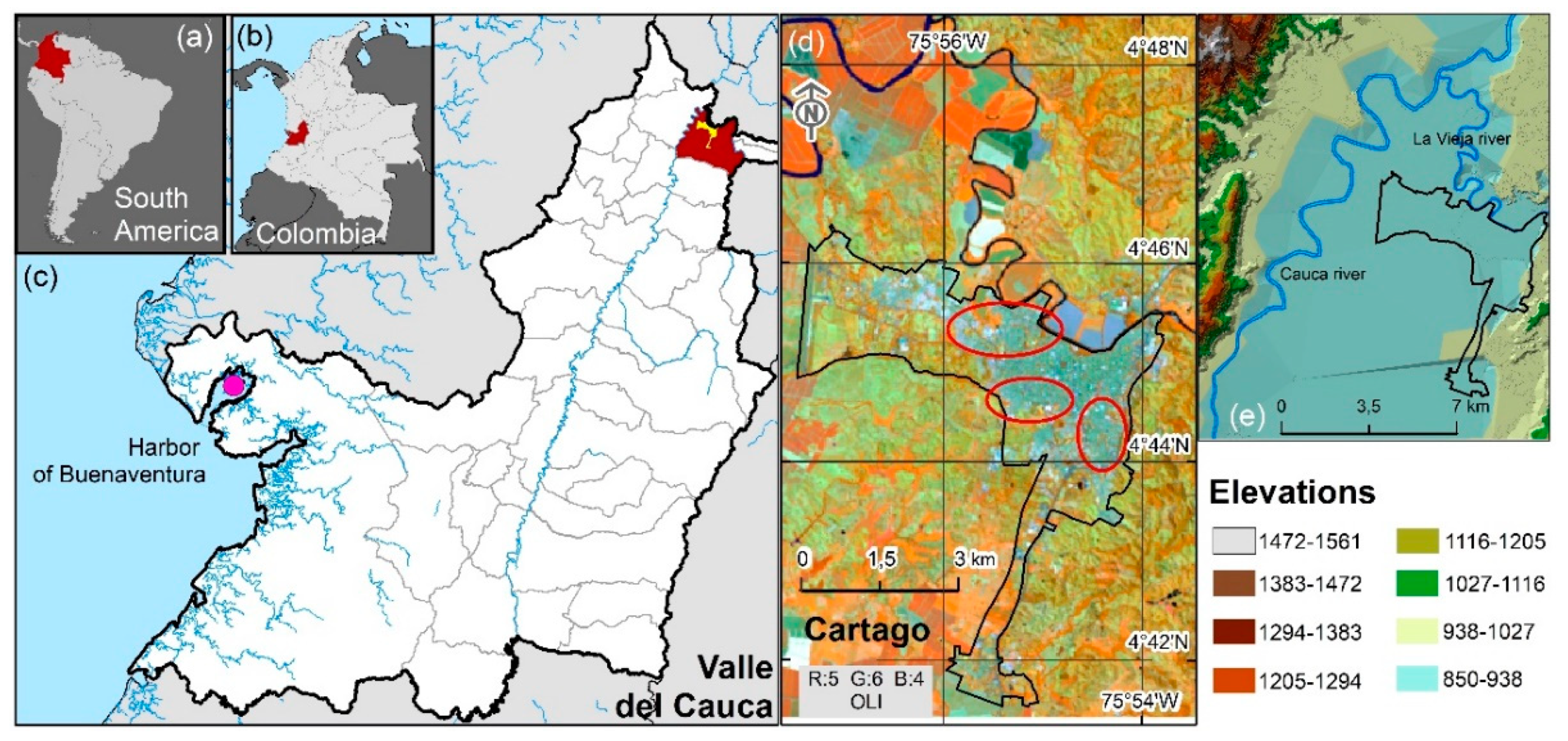
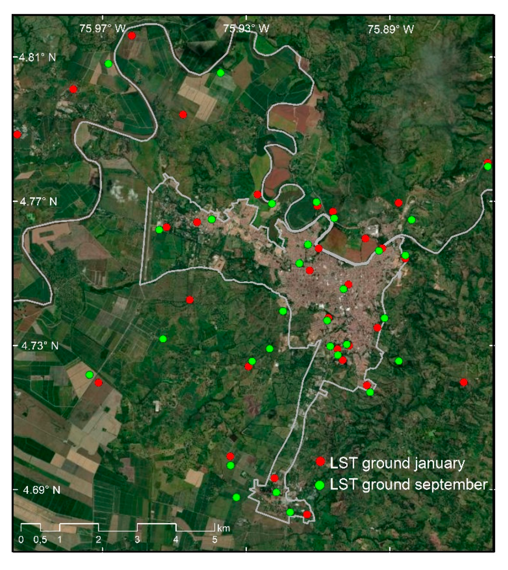
2.1. Study Area
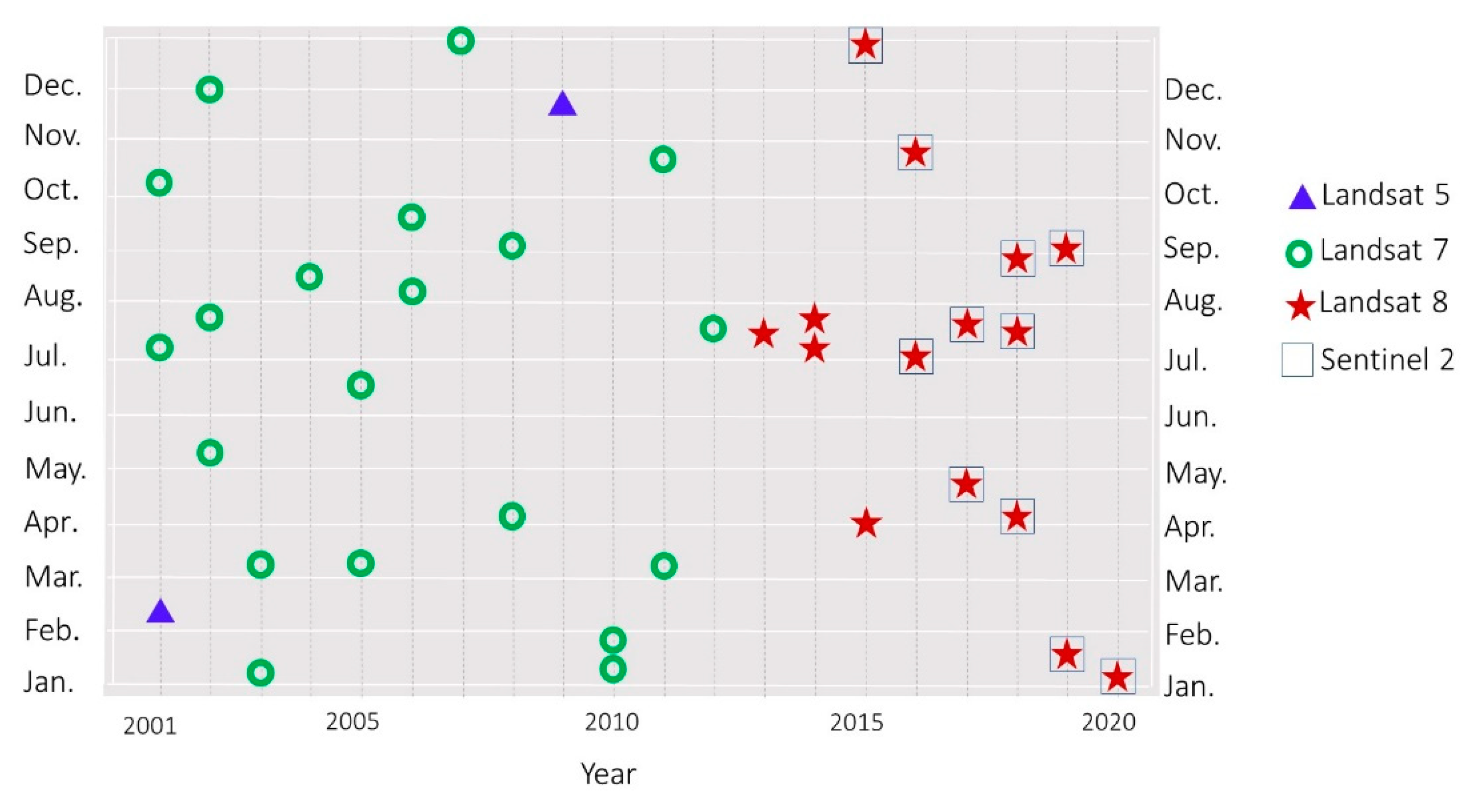
2.2. Data
2.3. Methods
2.3.1. Data Calibration
2.3.2. Definition and Extraction of Contributing Factors
- Energy exchange between latent and sensible heat is related to NDBI, since it detects impervious surfaces that reduce humidity and increase the average temperature of the environment [48].
- Temperature and vegetation maintain a spatially dependent relationship [49]. Vegetation reduces surface irradiation and increases humidity through physiological processes that allow energy exchange, while producing a cooling effect. In this sense, an index for measuring this photosynthetic activity is the NDVI.
- The presence of water bodies has a cooling effect on urban temperature [50]. In this scheme, the NDWI quantifies the water content in the vegetation, while suggesting a significant effect in reducing SUHI. Likewise, rivers play an important role as thermal regulators of urban climate, increasing the cooling potential through evaporation and facilitating airflow. Given that the urban center is the main point for the development of socioeconomic activities, two additional variables were considered to describe the expression of the proximity, i.e., the proximity map of the water body (PW) and the proximity map (PW) and the city center (PUC). A greater distance would imply a lower thermal intensity [51]. The proximity indices are computed by means of a Euclidean distance using the inverse weight distance operator in ArcGIS® (https://esri.com/, accessed on 20 October 2021).
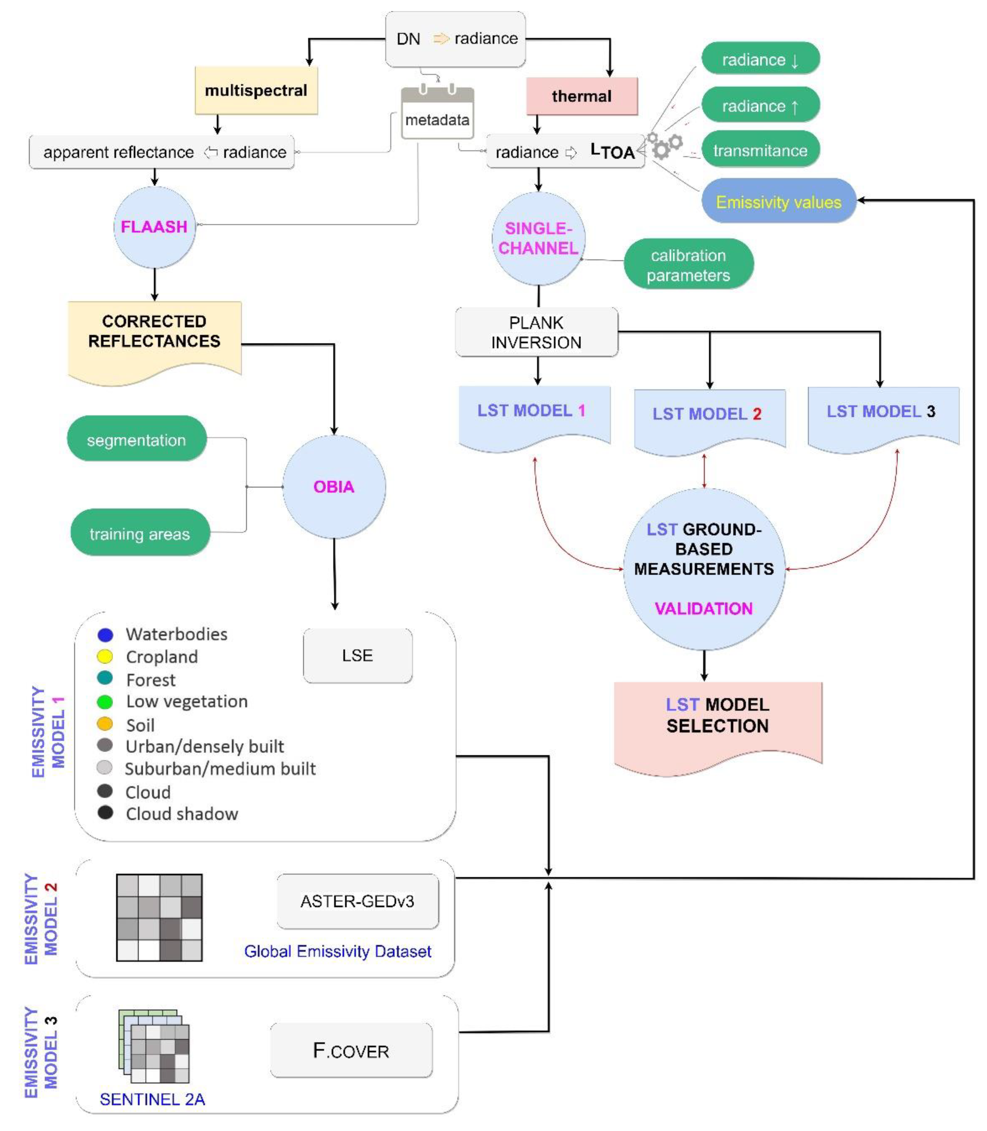
2.3.3. Estimation of Land Surface Temperature and Emissivity

| Land Cover | Emissivity | Reference |
|---|---|---|
| Waterbodies | 0.992 | FROM-GLC cited by [64] |
| Cropland | 0.971 | FROM-GLC cited by [64] |
| Forest | 0.995 | FROM-GLC cited by [64] |
| Low vegetation | 0.986 | Tan et al. [65] |
| Soil | 0.972 | Tan et al. [65] |
| Urban/densely built | 0.973 | FROM-GLC cited by [64] |
| Suburban/medium built | 0.971 | Tan et al. [65] |
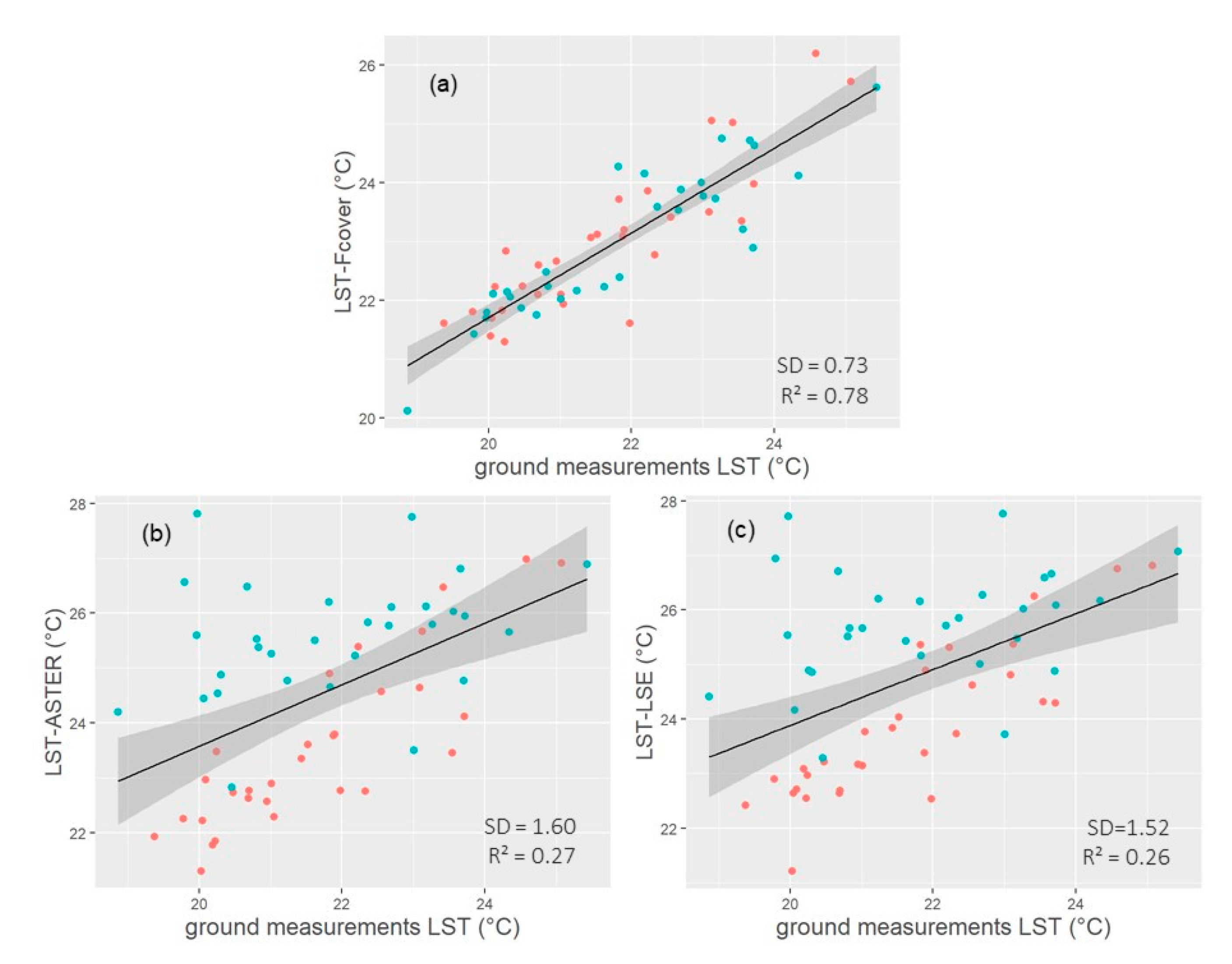
2.3.4. Assessment of the Land Surface Temperature Retrieved from L8TIRS B10
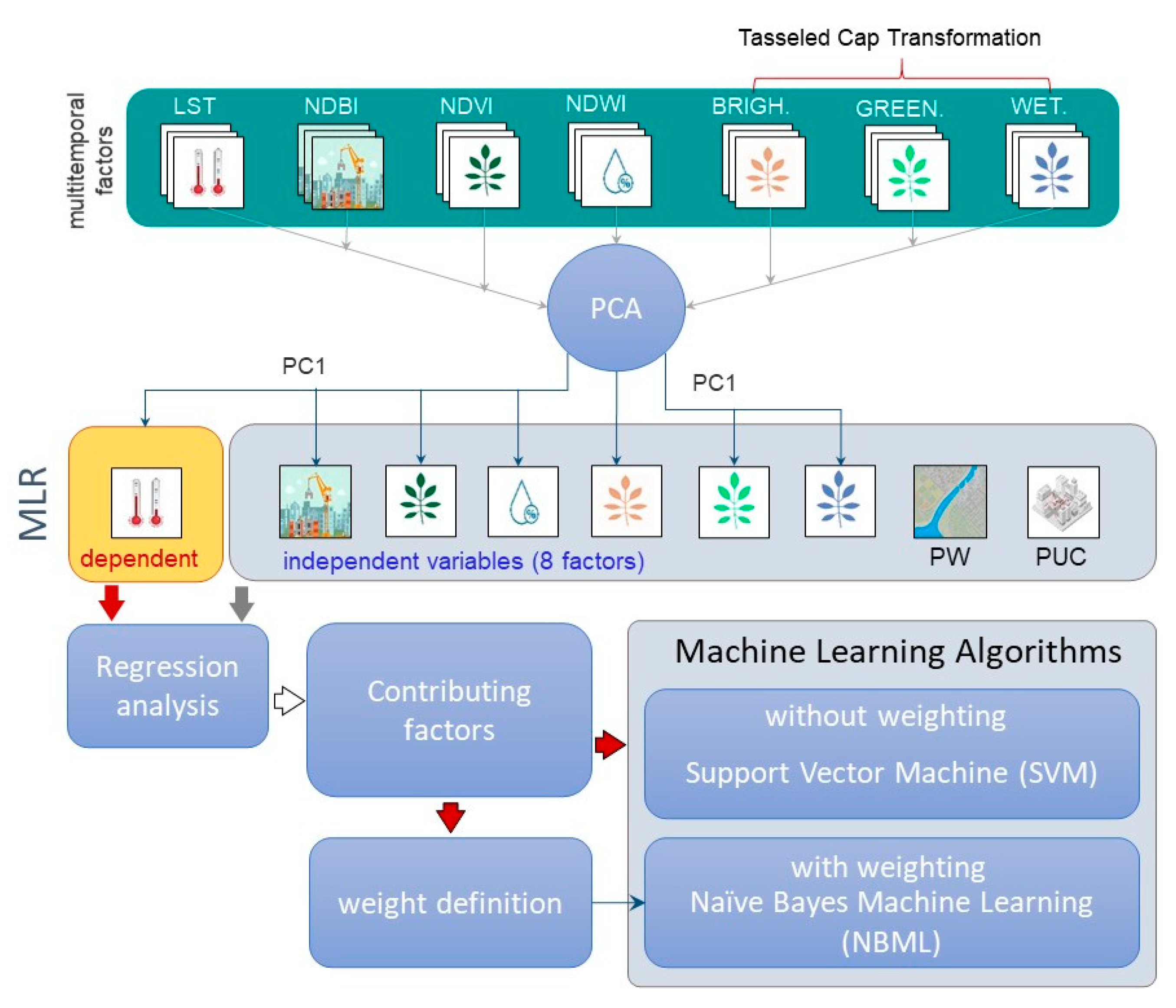
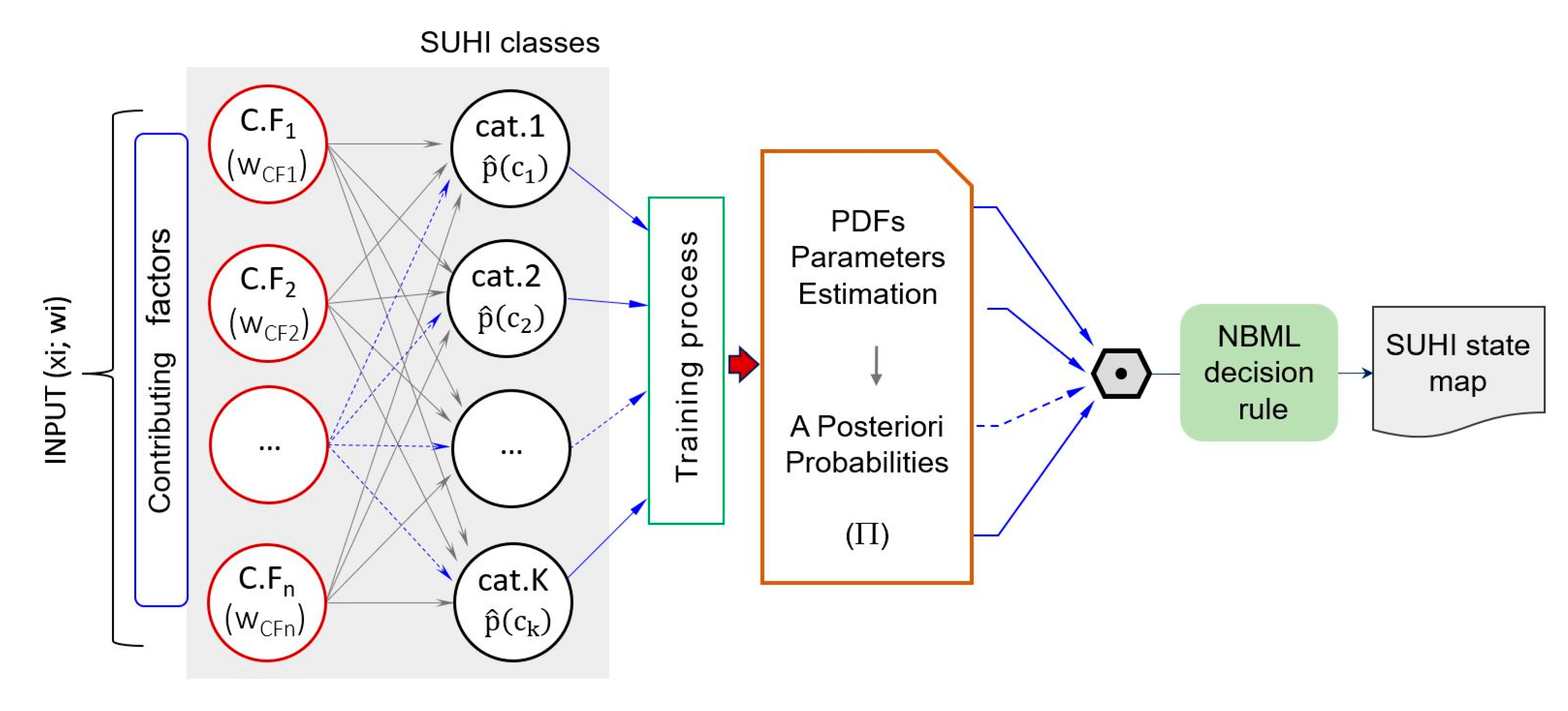
2.3.5. Modelling the SUHI Phenomenon
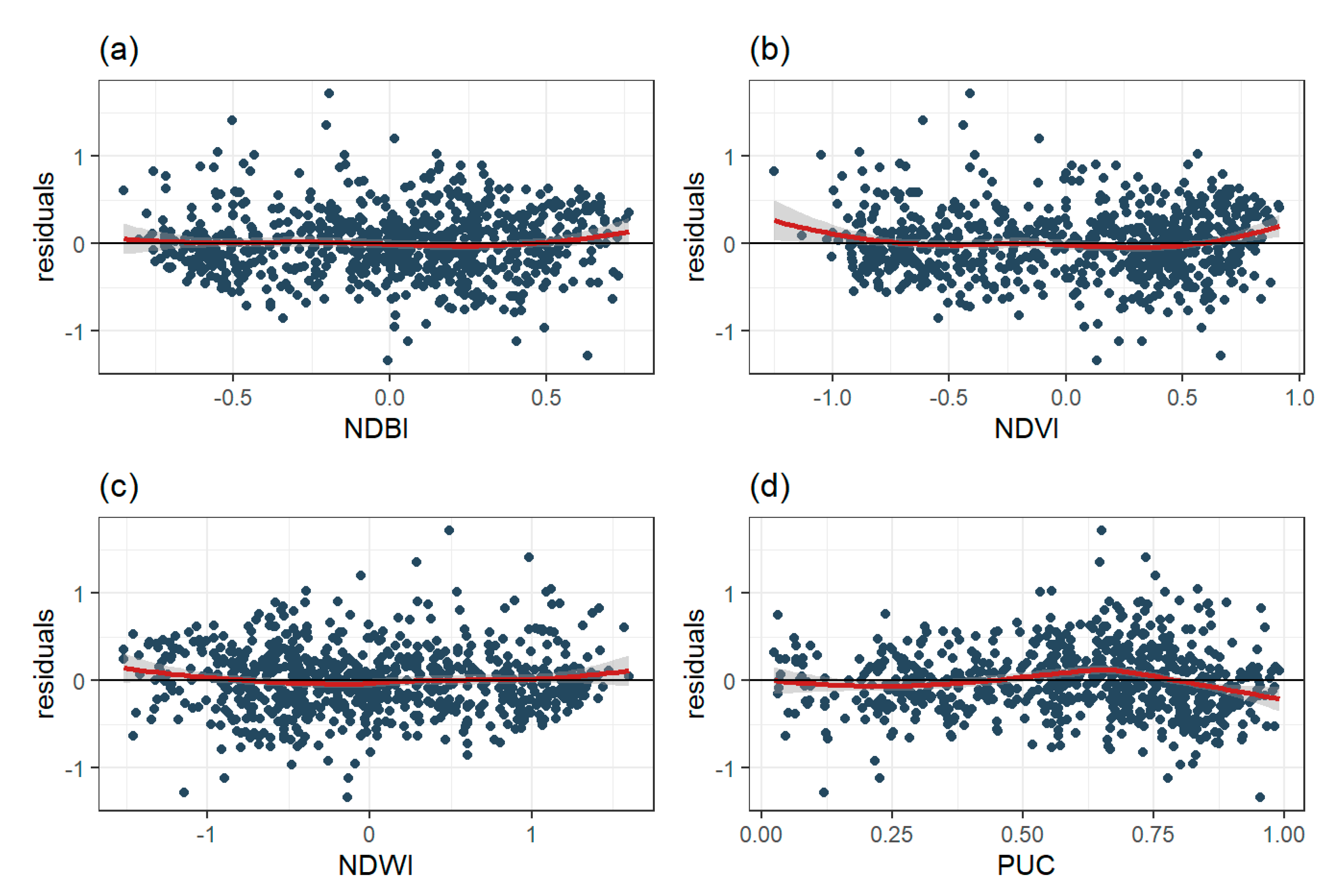
- Autocorrelation of a variable represents its self-dependence and implies redundant information that makes the estimator lose efficiency. The Durbin-Watson statistic is used to measure autocorrelation [75].
- The normality of a residuals guarantees a satisfactory representation of the model.
- Multicollinearity occurs when the predictor variables are highly correlated. Multicollinearity increases the variance, causing instability of the regression and thus increasing the standard error [76]. Multicollinearity is measured with the Variance Inflation Factor (VIF).
3. Results
3.1. Land Surface Temperature
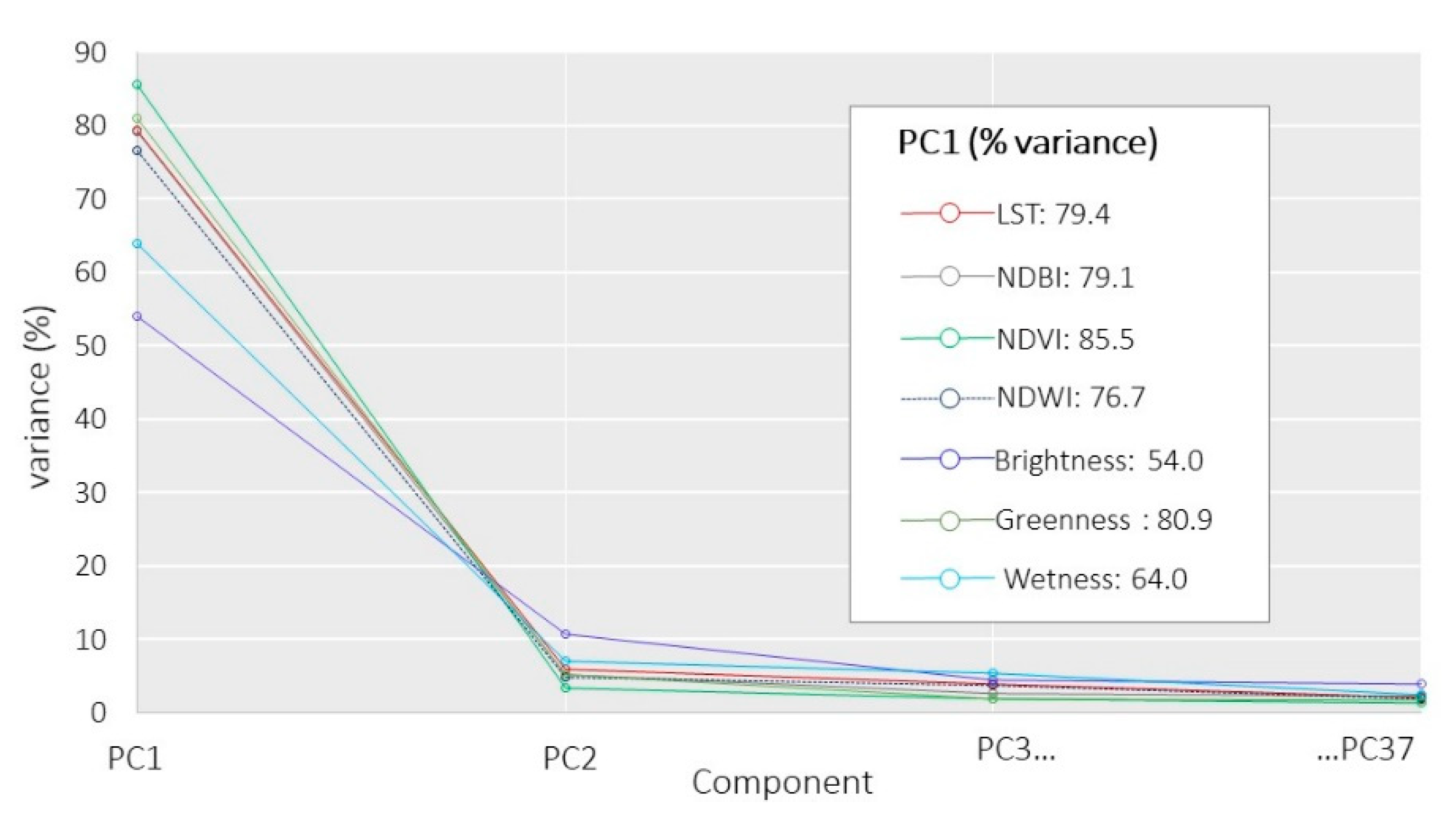
3.2. Principal Component Analysis
3.3. Multiple Linear Regression
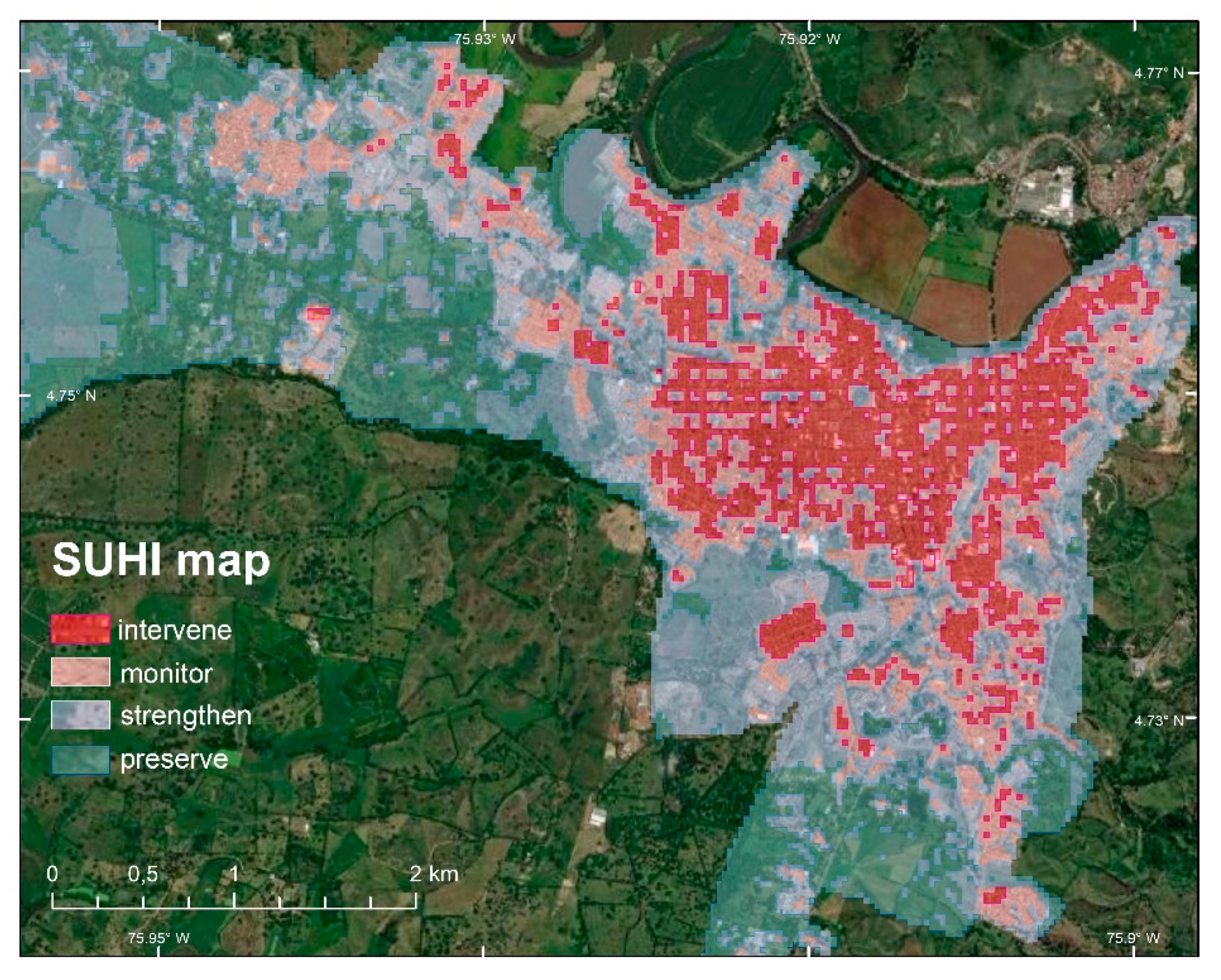
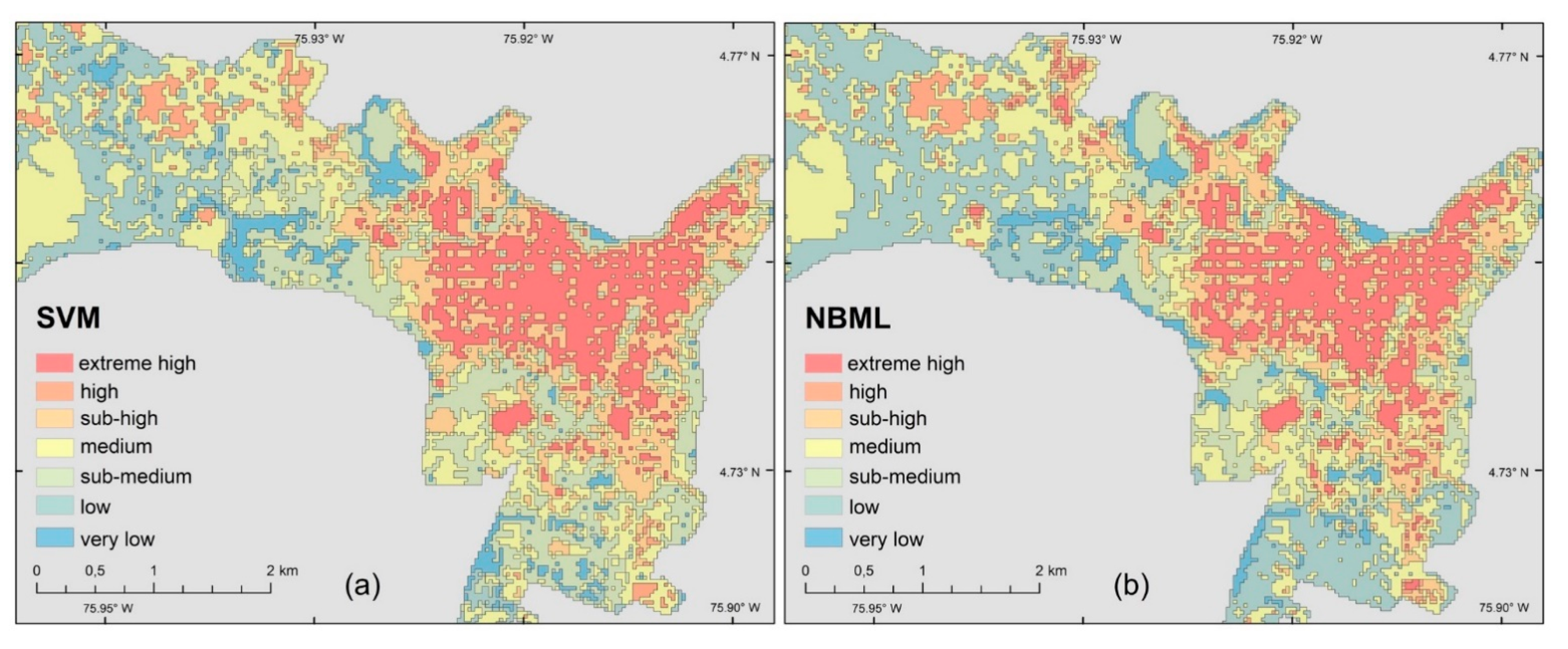
3.4. SUHI Modeling
4. Discussion
4.1. Sensitivity Analysis
4.2. Statistical Analyses
4.3. The SUHI Model
5. Conclusions
Author Contributions
Funding
Institutional Review Board Statement
Informed Consent Statement
Data Availability Statement
Conflicts of Interest
References
- Oke, T.R. The energetic basis of the urban heat island. Q. J. R. Meteorol. Soc. 1982, 108, 1–24. [Google Scholar] [CrossRef]
- Voogt, J.A.; Oke, T.R. Thermal remote sensing of urban climates. Remote Sens. Environ. 2003, 86, 370–384. [Google Scholar] [CrossRef]
- Schwarz, N.; Schlink, U.; Franck, U.; Großmann, K. Relationship of land surface and air temperatures and its implications for quantifying urban heat island indicators—An application for the city of Leipzig (Germany). Ecol. Indic. 2012, 18, 693–704. [Google Scholar] [CrossRef]
- Gubler, M.; Christen, A.; Remund, J.; Brönnimann, S. Evaluation and application of a low-cost measurement network to study intra-urban temperature differences during summer 2018 in Bern, Switzerland. Urban Clim. 2021, 37, 100817. [Google Scholar] [CrossRef]
- Chakraborty, T.C.; Lee, X.; Ermida, S.; Zhan, W. On the land emissivity assumption and Landsat-derived surface urban heat islands: A global analysis. Remote Sens. Environ. 2021, 265, 112682. [Google Scholar] [CrossRef]
- Sobrino, J.A.; Oltra-Carrió, R.; Sòria, G.; Jiménez-Muñoz, J.C.; Franch, B.; Hidalgo, V.; Mattar, C.; Julien, Y.; Cuenca, J.; Romaguera, M.; et al. Evaluation of the surface urban heat island effect in the city of Madrid by thermal remote sensing. Int. J. Remote Sens. 2013, 34, 3177–3192. [Google Scholar] [CrossRef]
- WMO Essential Climate Variables. Available online: https://public.wmo.int/en/programmes/global-climate-observing-system/essential-climate-variables (accessed on 18 October 2019).
- Zhou, D.; Xiao, J.; Bonafoni, S.; Berger, C.; Deilami, K.; Zhou, Y.; Frolking, S.; Yao, R.; Qiao, Z.; Sobrino, J.A. Satellite remote sensing of surface urban heat islands: Progress, challenges, and perspectives. Remote Sens. 2019, 11, 48. [Google Scholar] [CrossRef] [Green Version]
- Sekertekin, A.; Zadbagher, E. Simulation of future land surface temperature distribution and evaluating surface urban heat island based on impervious surface area. Ecol. Indic. 2021, 122, 107230. [Google Scholar] [CrossRef]
- Li, S.; Zhao, Z.; Miaomiao, X.; Wang, Y. Investigating spatial non-stationary and scale-dependent relationships between urban surface temperature and environmental factors using geographically weighted regression. Environ. Model. Softw. 2010, 25, 1789–1800. [Google Scholar] [CrossRef]
- Mei, C.-L.; Wang, N.; Zhang, W.X. Testing the importance of the explanatory variables in a mixed geographically weighted regression model. Environ. Plan. A 2006, 38, 587–598. [Google Scholar] [CrossRef]
- Senanayake, I.P.; Welivitiya, W.D.D.P.; Nadeeka, P.M. Remote sensing based analysis of urban heat islands with vegetation cover in Colombo city, Sri Lanka using Landsat-7 ETM + data. Urban Clim. 2013, 5, 19–35. [Google Scholar] [CrossRef]
- Bokaie, M.; Zarkesh, M.K.; Arasteh, P.D.; Hosseini, A. Assessment of Urban Heat Island based on the relationship between land surface temperature and Land Use/Land Cover in Tehran. Sustain. Cities Soc. 2016, 23, 94–104. [Google Scholar] [CrossRef]
- Chen, X.; Zhang, Y. Impacts of urban surface characteristics on spatiotemporal pattern of land surface temperature in Kunming of China. Sustain. Cities Soc. 2017, 32, 87–99. [Google Scholar] [CrossRef] [Green Version]
- Hereher, M.E. Effect of land use/cover change on land surface temperatures—The Nile Delta, Egypt. J. Afr. Earth Sci. 2017, 126, 75–83. [Google Scholar] [CrossRef]
- Shi, Y.; Xiang, Y.; Zhang, Y. Urban design factors influencing surface urban heat island in the high-density city of guangzhou based on the local climate zone. Sensors 2019, 19, 3459. [Google Scholar] [CrossRef] [PubMed] [Green Version]
- Song, J.; Wang, J.; Xia, X.; Lin, R.; Wang, Y.; Zhou, M.; Fu, D. Characterization of urban heat islands using city lights: Insights from modis and viirs dnb observations. Remote Sens. 2021, 13, 3180. [Google Scholar] [CrossRef]
- Parmentier, B. Characterization of land transitions patterns from multivariate time series using seasonal trend analysis and principal component analysis. Remote Sens. 2014, 6, 12639–12665. [Google Scholar] [CrossRef] [Green Version]
- Firozjaei, M.K.; Alavipanah, S.K.; Liu, H.; Sedighi, A.; Mijani, N.; Kiavarz, M.; Weng, Q. A PCA-OLS model for assessing the impact of surface biophysical parameters on land surface temperature variations. Remote Sens. 2019, 11, 2094. [Google Scholar] [CrossRef] [Green Version]
- Lemus-Canovas, M.; Martin-Vide, J.; Moreno-Garcia, M.C.; Lopez-Bustins, J.A. Estimating Barcelona’s metropolitan daytime hot and cold poles using Landsat-8 Land Surface Temperature. Sci. Total Environ. 2020, 699, 134307. [Google Scholar] [CrossRef]
- Shams, S.R.; Jahani, A.; Kalantary, S.; Moeinaddini, M.; Khorasani, N. Artificial intelligence accuracy assessment in NO2 concentration forecasting of metropolises air. Sci. Rep. 2021, 11, 1805. [Google Scholar] [CrossRef]
- Wicki, A.; Parlow, E. Multiple regression analysis for unmixing of surface temperature data in an urban environment. Remote Sens. 2017, 9, 684. [Google Scholar] [CrossRef] [Green Version]
- Zheng, Y.; Li, Y.; Hou, H.; Murayama, Y.; Wang, R.; Hu, T. Quantifying the cooling effect and scale of large inner-city lakes based on landscape patterns: A case study of hangzhou and nanjing. Remote Sens. 2021, 13, 1526. [Google Scholar] [CrossRef]
- Deng, Y.; Chen, R.; Xie, Y.; Xu, J.; Yang, J.; Liao, W. Exploring the impacts and temporal variations of different building roof types on surface urban heat island. Remote Sens. 2021, 13, 2840. [Google Scholar] [CrossRef]
- Oliveira, A.; Lopes, A.; Niza, S.; Soares, A. An urban energy balance-guided machine learning approach for synthetic nocturnal surface Urban Heat Island prediction: A heatwave event in Naples. Sci. Total Environ. 2022, 805, 150130. [Google Scholar] [CrossRef] [PubMed]
- Hassan, T.; Zhang, J.; Prodhan, F.A.; Pangali Sharma, T.P.; Bashir, B. Surface urban heat islands dynamics in response to lulc and vegetation across south asia (2000–2019). Remote Sens. 2021, 13, 3177. [Google Scholar] [CrossRef]
- Núñez-Peiró, M.; Mavrogianni, A.; Symonds, P.; Sánchez-Guevara Sánchez, C.; Neila González, F.J. Modelling long-term urban temperatures with less training data: A comparative study using neural networks in the city of Madrid. Sustainability 2021, 13, 8143. [Google Scholar] [CrossRef]
- Kwak, Y.; Park, C.; Deal, B. Discerning the success of sustainable planning: A comparative analysis of urban heat island dynamics in Korean new towns. Sustain. Cities Soc. 2020, 61, 102341. [Google Scholar] [CrossRef]
- Yoo, S. Investigating important urban characteristics in the formation of urban heat islands: A machine learning approach. J. Big Data 2018, 5, 2. [Google Scholar] [CrossRef] [Green Version]
- Voelkel, J.; Shandas, V. Towards systematic prediction of urban heat islands: Grounding measurements, assessing modeling techniques. Climate 2017, 5, 41. [Google Scholar] [CrossRef] [Green Version]
- Zumwald, M.; Knüsel, B.; Bresch, D.N.; Knutti, R. Mapping urban temperature using crowd-sensing data and machine learning. Urban Clim. 2021, 35, 100739. [Google Scholar] [CrossRef]
- Kafy, A.-A.; Faisal, A.A.; Rahman, M.S.; Islam, M.; Al Rakib, A.; Islam, M.A.; Khan, M.H.H.; Sikdar, M.S.; Sarker, M.H.S.; Mawa, J.; et al. Prediction of seasonal urban thermal field variance index using machine learning algorithms in Cumilla, Bangladesh. Sustain. Cities Soc. 2021, 64, 102542. [Google Scholar] [CrossRef]
- Shi, H.; Xian, G.; Auch, R.; Gallo, K.; Zhou, Q. Urban Heat Island and its regional impacts using remotely sensed thermal data—A review of recent developments and methodology. Land 2021, 10, 867. [Google Scholar] [CrossRef]
- Alves, E.; Anjos, M.; Galvani, E. Surface urban heat island in middle city: Spatial and temporal characteristics. Urban Sci. 2020, 4, 54. [Google Scholar] [CrossRef]
- Chakraborty, T.; Hsu, A.; Manya, D.; Sheriff, G. A spatially explicit surface urban heat island database for the United States: Characterization, uncertainties, and possible applications. ISPRS J. Photogramm. Remote Sens. 2020, 168, 74–88. [Google Scholar] [CrossRef]
- Wang, H.; Zhang, Y.; Tsou, J.Y.; Li, Y. Surface urban heat island analysis of shanghai (China) based on the change of land use and land cover. Sustainability 2017, 9, 1538. [Google Scholar] [CrossRef] [Green Version]
- DANE Departamento Administrativo Nacional de Estadística. Available online: https://www.dane.gov.co/ (accessed on 12 December 2020).
- Municipio de Cartago Valle del Cauca—Alcaldía de Cartago. Available online: http://www.cartago.gov.co/pot-vigente (accessed on 15 January 2018).
- Sobrino, J.A.; Raissouni, N.; Li, Z. A Comparative study of land surface emissivity retrieval from NOAA data. Remote Sens. Environ. 2001, 75, 256–266. [Google Scholar] [CrossRef]
- Valor, E.; Caselles, V. Mapping land surface emissivity from NDVI: Application to European, African, and South American areas. Remote Sens. Environ. 1996, 57, 167–184. [Google Scholar] [CrossRef]
- USGS Landsat 8 (L8) Data Users Handbook. Available online: https://www.usgs.gov/media/files/landsat-8-data-users-handbook (accessed on 7 January 2020).
- Tarawally, M.; Xu, W.; Hou, W.; Mushore, T.D. Comparative analysis of responses of land surface temperature to long-term land use/cover changes between a coastal and Inland City: A case of Freetown and Bo Town in Sierra Leone. Remote Sens. 2018, 10, 112. [Google Scholar] [CrossRef] [Green Version]
- Kaufman, Y.J.; Tanré, D.; Gordon, H.R.; Nakajima, T.; Lenoble, J.; Frouin, R.; Grassl, H.; Herman, B.M.; King, M.D.; Teillet, P.M. Passive remote sensing of tropospheric aerosol and atmospheric correction for the aerosol effect. J. Geophys. Res. Atmos. 1997, 102, 16815–16830. [Google Scholar] [CrossRef] [Green Version]
- Zha, Y.; Gao, J.; Ni, S. Use of normalized difference built-up index in automatically mapping urban areas from TM imagery. Int. J. Remote Sens. 2003, 24, 583–594. [Google Scholar] [CrossRef]
- Tucker, C.J. Red and photographic infrared linear combinations for monitoring vegetation. Remote Sens. Environ. 1979, 8, 127–150. [Google Scholar] [CrossRef] [Green Version]
- Gao, B.-C. Naval Research Laboratory, 4555 Overlook Ave. Remote Sens. Environ. 1996, 58, 257–266. [Google Scholar] [CrossRef]
- Baig, M.H.A.; Zhang, L.; Shuai, T.; Tong, Q. Derivation of a tasselled cap transformation based on Landsat 8 at-satellite reflectance. Remote Sens. Lett. 2014, 5, 423–431. [Google Scholar] [CrossRef]
- Zhang, Y.; Odeh, I.O.A.; Han, C. Bi-temporal characterization of land surface temperature in relation to impervious surface area, NDVI and NDBI, using a sub-pixel image analysis. Int. J. Appl. Earth Obs. Geoinf. 2009, 11, 256–264. [Google Scholar] [CrossRef]
- Karnieli, A.; Ohana-Levi, N.; Silver, M.; Paz-Kagan, T.; Panov, N.; Varghese, D.; Chrysoulakis, N.; Provenzale, A. Spatial and seasonal patterns in vegetation growth-limiting factors over Europe. Remote Sens. 2019, 11, 2406. [Google Scholar] [CrossRef] [Green Version]
- Yang, C.; He, X.; Yu, L.; Yang, J.; Yan, F.; Bu, K.; Chang, L.; Zhang, S. The cooling effect of urban parks and its monthly variations in a snow climate city. Remote Sens. 2017, 9, 1066. [Google Scholar] [CrossRef] [Green Version]
- Hathway, E.A.; Sharples, S. The interaction of rivers and urban form in mitigating the Urban Heat Island effect: A UK case study. Build. Environ. 2012, 58, 14–22. [Google Scholar] [CrossRef] [Green Version]
- Olioso, A. Simulating the relationship between thermal emissivity and the Normalized Difference Vegetation Index. Int. J. Remote Sens. 1995, 16, 3211–3216. [Google Scholar] [CrossRef]
- Wittich, K.-P. Some simple relationships between land-surface emissivity, greenness and the plant cover fraction for use in satellite remote sensing. Int. J. Biometeorol. 1997, 41, 58–64. [Google Scholar] [CrossRef]
- Mallick, J.; Singh, C.K.; Shashtri, S.; Rahman, A.; Mukherjee, S. Land surface emissivity retrieval based on moisture index from LANDSAT TM satellite data over heterogeneous surfaces of Delhi city. Int. J. Appl. Earth Obs. Geoinf. 2012, 19, 348–358. [Google Scholar] [CrossRef]
- Bacour, C.; Baret, F.; Béal, D.; Weiss, M.; Pavageau, K. Neural network estimation of LAI, fAPAR, fCover and LAI × Cab, from top of canopy MERIS reflectance data: Principles and validation. Remote Sens. Environ. 2006, 105, 313–325. [Google Scholar] [CrossRef]
- Weiss, M.; Baret, F. S2ToolBox Level 2 Products: LAI, FAPAR, FCOVER Version 1.1. 2016. Available online: https://step.esa.int/docs/extra/ATBD_S2ToolBox_L2B_V1.1.pdf (accessed on 15 December 2019).
- USGS Landsat 8 Thermal Infrared Sensor (TIRS) Calibration Notices. Available online: https://www.usgs.gov/land-resources/nli/landsat/landsat-8-oli-and-tirs-calibration-notices (accessed on 18 June 2020).
- Sekertekin, A.; Bonafoni, S. Land surface temperature retrieval from Landsat 5, 7, and 8 over rural areas: Assessment of different retrieval algorithms and emissivity models and toolbox implementation. Remote Sens. 2020, 12, 294. [Google Scholar] [CrossRef] [Green Version]
- Barsi, J.A.; Schott, J.R.; Palluconi, F.D.; Hook, S.J. Validation of a web-based atmospheric correction tool for single thermal band instruments. In Proceedings of the Earth Observing Systems X, SPIE, San Diego, CA, USA, 22 August 2005; Volume 5882, p. 58820E. [Google Scholar]
- Yue, W.; Xu, J.; Tan, W.; Xu, L. The relationship between land surface temperature and NDVI with remote sensing: Application to Shanghai Landsat 7 ETM + data. Int. J. Remote Sens. 2007, 28, 3205–3226. [Google Scholar] [CrossRef]
- Hulley, G.C.; Hook, S.J.; Abbott, E.; Malakar, N.; Islam, T.; Abrams, M. The aster global emissivity dataset (ASTER GED): Mapping Earth’s emissivity at 100 meter spatial scale. Geophys. Res. Lett. 2015, 42, 7966–7976. [Google Scholar] [CrossRef]
- Park, J.; Jang, S.; Hong, R.; Suh, K.; Song, I. Development of land cover classification model using AI based fusionnet network. Remote Sens. 2020, 12, 3171. [Google Scholar] [CrossRef]
- Lu, D.; Hetrick, S.; Moran, E. Land cover classification in a complex urban-rural landscape with quickbird imagery. Photogramm. Eng. Remote Sens. 2010, 76, 1159–1168. [Google Scholar] [CrossRef] [Green Version]
- Du, C.; Ren, H.; Qin, Q.; Meng, J.; Zhao, S. A practical split-window algorithm for estimating land surface temperature from landsat 8 data. Remote Sens. 2015, 7, 647–665. [Google Scholar] [CrossRef] [Green Version]
- Tan, K.; Liao, Z.; Du, P.; Wu, L. Land surface temperature retrieval from Landsat 8 data and validation with geosensor network. Front. Earth Sci. 2017, 11, 20–34. [Google Scholar] [CrossRef]
- Hulley, G.C.; Hook, S.J. Generating consistent land surface temperature and emissivity products between ASTER and MODIS data for earth science research. IEEE Trans. Geosci. Remote Sens. 2011, 49, 1304–1315. [Google Scholar] [CrossRef]
- Sobrino, J.A.; Jiménez-Muñoz, J.C.; Sòria, G.; Romaguera, M.; Guanter, L.; Moreno, J.; Plaza, A.; Martínez, P. Land surface emissivity retrieval from different VNIR and TIR sensors. IEEE Trans. Geosci. Remote Sens. 2008, 46, 316–327. [Google Scholar] [CrossRef]
- Jiménez-Muñoz, J.C.; Sobrino, J.A.; Skokovi, D.; Mattar, C.; Cristóbal, J.; Bands, A.L.-T. Land surface temperature retrieval methods from Landsat-8 thermal infrared sensor data. IEEE Geosci. Remote Sens. Lett. 2014, 11, 1840–1843. [Google Scholar] [CrossRef]
- Carlson, T.N.; Ripley, D.A. On the relation between NDVI, fractional vegetation cover, and leaf area index. Remote Sens. Environ. 1997, 62, 241–252. [Google Scholar] [CrossRef]
- Jiménez-Muñoz, J.C.; Cristobal, J.; Sobrino, J.A.; Sòria, G.; Ninyerola, M.; Pons, X. Revision of the single-channel algorithm for land surface temperature retrieval from landsat thermal-infrared data. IEEE Trans. Geosci. Remote Sens. 2009, 47, 339–349. [Google Scholar] [CrossRef]
- Li, Z.-L.; Tang, B.-H.; Wu, H.; Ren, H.; Yan, G.; Wan, Z.; Trigo, I.F.; Sobrino, J.A. Satellite-derived land surface temperature: Current status and perspectives. Remote Sens. Environ. 2013, 131, 14–37. [Google Scholar] [CrossRef] [Green Version]
- Rasul, A.; Balzter, H.; Smith, C.; Remedios, J.; Adamu, B.; Sobrino, J.; Srivanit, M.; Weng, Q. A review on remote sensing of urban heat and cool islands. Land 2017, 6, 38. [Google Scholar] [CrossRef] [Green Version]
- Machidon, A.L.; Del Frate, F.; Picchiani, M.; Machidon, O.M.; Ogrutan, P.L. Geometrical approximated principal component analysis for hyperspectral image analysis. Remote Sens. 2020, 12, 1698. [Google Scholar] [CrossRef]
- Adame-Campos, R.L.; Ghilardi, A.; Gao, Y.; Paneque-Gálvez, J.; Mas, J.F. Variables selection for aboveground biomass estimations using satellite data: A comparison between relative importance approach and stepwise Akaike’s information criterion. ISPRS Int. J. Geo-Inf. 2019, 8, 245. [Google Scholar] [CrossRef] [Green Version]
- Hanssens, D.M.; Parsons, L.J.; Schultz, R.L. Parameter estimation and model testing. In International Series in Quantitative Marketing; Springer: Boston, MA, USA, 2002; pp. 183–248. [Google Scholar]
- Harrell, F. Regression Modeling Strategies: With Applications to Linear Models, Logistic and Ordinal Regression and Survival Analysis, 2nd ed.; Springer: Berlin/Heidelberg, Germany, 2015; ISBN 9783319194240. [Google Scholar]
- Rahman, S.M.A.K.; Sathik, M.M.; Kannan, K.S. Multiple linear regression models in outlier detection. Int. J. Res. Comput. Sci. 2012, 2, 23–28. [Google Scholar] [CrossRef]
- Zhao, X.; Zhang, Y.; Xie, S.; Qin, Q.; Wu, S.; Luo, B. Outlier detection based on residual histogram preference for geometric multi-model fitting. Sensors 2020, 20, 3037. [Google Scholar] [CrossRef]
- Wilks, D.S. Statistical Methods in the Atmospheric Sciences, 4th ed.; Elsevier: Amsterdam, The Netherlands, 2019; ISBN 9780128158234. [Google Scholar]
- Noi, P.T.; Kappas, M. Comparison of random forest, k-nearest neighbor, and support vector machine classifiers for land cover classification using Sentinel-2 Imagery. Sensors 2017, 18, 18. [Google Scholar] [CrossRef] [Green Version]
- Barca, E.; Castrignanò, A.; Ruggieri, S.; Rinaldi, M. A new supervised classifier exploiting spectral-spatial information in the Bayesian framework. Int J. Appl Earth Obs. Geoinf. 2020, 86, 101990. [Google Scholar] [CrossRef]
- Tian, S.; Zhang, X.; Tian, J.; Sun, Q. Random forest classification of wetland landcovers from multi-sensor data in the arid region of Xinjiang, China. Remote Sens. 2016, 8, 954. [Google Scholar] [CrossRef] [Green Version]
- Lv, Z.Y.; He, H.; Benediktsson, J.A.; Huang, H. A generalized image scene decomposition-based system for supervised classification of very high resolution remote sensing imagery. Remote Sens. 2016, 8, 814. [Google Scholar] [CrossRef] [Green Version]
- Park, D. Image classification using naïve bayes classifier. Int. J. Comput. Sci. Electron. Eng. 2016, 4, 135–139. [Google Scholar]
- Judah, A.; Hu, B. The integration of multi-source remotely-sensed data in support of the classification of wetlands. Remote Sens. 2019, 11, 1537. [Google Scholar] [CrossRef] [Green Version]
- Zhang, H.; Jiang, L.; Yu, L. Class-specific attribute value weighting for Naive Bayes. Inf. Sci. 2020, 508, 260–274. [Google Scholar] [CrossRef]
- Jenks, G.F. The data model concept in statistical mapping. Int. Yearb. Cartogr. 1967, 7, 186–190. [Google Scholar]
- Szymanowski, M.; Kryza, M. Local regression models for spatial interpolation of urban heat island-an example from Wrocław, SW Poland. Theor. Appl. Climatol. 2012, 108, 53–71. [Google Scholar] [CrossRef] [Green Version]
- Ogashawara, I.; Bastos, V. A quantitative approach for analyzing the relationship between Urban Heat Islands and Land Cover. Remote Sens. 2012, 4, 3596–3618. [Google Scholar] [CrossRef] [Green Version]
- Zhang, X.; Estoque, R.C.; Murayama, Y. An urban heat island study in Nanchang City, China based on land surface temperature and social-ecological variables. Sustain. Cities Soc. 2017, 32, 557–568. [Google Scholar] [CrossRef]
- Guha, S.; Govil, H.; Diwan, P. Analytical study of seasonal variability in land surface temperature with normalized difference vegetation index, normalized difference water index, normalized difference built-up index, and normalized multiband drought index. J. Appl. Remote Sens. 2019, 13, 024518. [Google Scholar] [CrossRef] [Green Version]
- Cruz, J.A.; Santos, J.A.; Blanco, A. Spatial disaggregation of Landsat-derived land surface temperature over a heterogeneous urban landscape using planetscope image derivatives. Int. Arch. Photogramm. Remote Sens. Spat. Inf. Sci. 2020, 43, 115–122. [Google Scholar] [CrossRef]
- Duan, S.-B.; Li, Z.-L.; Wang, C.; Zhang, S.; Tang, B.-H.; Leng, P.; Gao, M.F. Land-surface temperature retrieval from Landsat 8 single-channel thermal infrared data in combination with NCEP reanalysis data and ASTER GED product. Int. J. Remote Sens. 2018, 40, 1763–1778. [Google Scholar] [CrossRef]
- Malakar, N.K.; Hulley, G.C.; Hook, S.J.; Laraby, K.; Cook, M.; Schott, J.R. An operational land surface temperature product for landsat thermal data: Methodology and validation. IEEE Trans. Geosci. Remote Sens. 2018, 56, 5717–5735. [Google Scholar] [CrossRef]
- Liu, C.; Li, Y. Spatio-temporal features of urban heat island and its relationship with land use/cover in mountainous city: A case study in Chongqing. Sustainability 2018, 10, 1943. [Google Scholar] [CrossRef] [Green Version]
- Nill, L.; Ullmann, T.; Kneisel, C.; Sobiech-Wolf, J.; Baumhauer, R. Assessing spatiotemporal variations of landsat land surface temperature and multispectral indices in the Arctic Mackenzie Delta Region between 1985 and 2018. Remote Sens. 2019, 11, 2329. [Google Scholar] [CrossRef] [Green Version]
- Dos-Santos, A.R.; de Oliveira, F.S.; da Silva, A.G.; Gleriani, J.M.; Gonçalves, W.; Moreira, G.L.; Silva, F.G.; Branco, E.R.F.; Moura, M.M.; da Silva, R.G.; et al. Spatial and temporal distribution of urban heat islands. Sci. Total Environ. 2017, 605–606, 946–956. [Google Scholar] [CrossRef]
- Guha, S.; Govil, H.; Dey, A.; Gill, N. Analytical study of land surface temperature with NDVI and NDBI using Landsat 8 OLI and TIRS data in Florence and Naples city, Italy. Eur. J. Remote Sens. 2018, 51, 667–678. [Google Scholar] [CrossRef]
- Ibrahim, G.R.F. Urban land use land cover changes and their effect on land surface temperature: Case study using Dohuk City in the Kurdistan Region of Iraq. Climate 2017, 5, 13. [Google Scholar] [CrossRef] [Green Version]
- Bonafoni, S.; Keeratikasikorn, C. Land surface temperature and urban density: Multiyear modeling and relationship analysis using modis and landsat data. Remote Sens. 2018, 10, 1471. [Google Scholar] [CrossRef] [Green Version]
- Molina, I.; Martinez, E.; Morillo, C.; Velasco, J.; Jara, A. Assessment of data fusion algorithms for earth observation change detection processes. Sensors 2016, 16, 1621. [Google Scholar] [CrossRef] [PubMed] [Green Version]
- Renard, F.; Alonso, L.; Fitts, Y.; Hadjiosif, A.; Comby, J. Evaluation of the effect of urban redevelopment on surface urban heat islands. Remote Sens. 2019, 11, 299. [Google Scholar] [CrossRef] [Green Version]
- Alshayeb, M.J.; Chang, J.D. Variations of PV panel performance installed over a vegetated roof and a conventional black roof. Energies 2018, 11, 1110. [Google Scholar] [CrossRef] [Green Version]
- Grilo, F.; Pinho, P.; Aleixo, C.; Catita, C.; Silva, P.; Lopes, N.; Freitas, C.; Santos-reis, M.; Mcphearson, T.; Branquinho, C. Using green to cool the gre: Modelling the cooling effect of green spaces with a high spatial resolution. Sci. Total Environ. 2020, 724, 138182. [Google Scholar] [CrossRef] [PubMed]
- U.S. Environmental Protection Agency. “Cool Pavements”. Reducing Urban Heat Islands: Compendium of Strategies. 2012. Available online: https://www.epa.gov/heat-islands/heat-island-compendium (accessed on 1 June 2021).


| Temperature Grade | Range |
|---|---|
| Extreme high temperature (EHT) | TS > Ta + 2SD |
| High temperature (HT) | Ta + SDTS ≤ Ta + 2SD |
| Sub-high temperature (SHT) | Ta + SD/2TS ≤ Ta + SD |
| Medium temperature (MT) | Ta − SD/2TS ≤ Ta + SD/2 |
| Sub-medium temperature (SMT) | Ta − SDTS ≤ Ta − SD/2 |
| Low temperature (LT) | Ta − 2SDTS ≤ Ta − SD |
| Sub-low temperature (SLT) | TS < Ta + 2SD |
| Factors | Estimate | SD | t Value | p (>t |0.05|) |
|---|---|---|---|---|
| (Intercept) | 0.29 | 0.01 | 34.79 | <0.001 |
| NDBI | 0.48 | 0.05 | 9.91 | <0.001 |
| NDVI | 0.21 | 0.02 | 13.21 | <0.001 |
| NDWI | −0.61 | 0.03 | −23.65 | <0.001 |
| PUC | −0.51 | 0.01 | −39.60 | <0.001 |
| Autocorrelation | Normality | Multicollinearity (VIF) | |||||
|---|---|---|---|---|---|---|---|
| D-W | p-Value | K-S | p-Value | NDBI | NDVI | NDWI | PUC |
| 2.00 | 0.80 | 0.02 | <0.001 | 45.03 | 9.12 | 45.75 | 1.26 |
| Factor | Standardized Coefficients | Weighted Contribution (%) |
| NDBI | 0.21 | 21.38 |
| NDVI | 0.13 | 12.84 |
| NDWI | −0.51 | 51.46 |
| PUC | −0.14 | 14.32 |
| Algorithm | Kappa Index | Overall Accuracy |
|---|---|---|
| SVM | 0.88 | 0.88 |
| NBML | 0.94 | 0.95 |
Publisher’s Note: MDPI stays neutral with regard to jurisdictional claims in published maps and institutional affiliations. |
© 2021 by the authors. Licensee MDPI, Basel, Switzerland. This article is an open access article distributed under the terms and conditions of the Creative Commons Attribution (CC BY) license (https://creativecommons.org/licenses/by/4.0/).
Share and Cite
Garzón, J.; Molina, I.; Velasco, J.; Calabia, A. A Remote Sensing Approach for Surface Urban Heat Island Modeling in a Tropical Colombian City Using Regression Analysis and Machine Learning Algorithms. Remote Sens. 2021, 13, 4256. https://doi.org/10.3390/rs13214256
Garzón J, Molina I, Velasco J, Calabia A. A Remote Sensing Approach for Surface Urban Heat Island Modeling in a Tropical Colombian City Using Regression Analysis and Machine Learning Algorithms. Remote Sensing. 2021; 13(21):4256. https://doi.org/10.3390/rs13214256
Chicago/Turabian StyleGarzón, Julián, Iñigo Molina, Jesús Velasco, and Andrés Calabia. 2021. "A Remote Sensing Approach for Surface Urban Heat Island Modeling in a Tropical Colombian City Using Regression Analysis and Machine Learning Algorithms" Remote Sensing 13, no. 21: 4256. https://doi.org/10.3390/rs13214256
APA StyleGarzón, J., Molina, I., Velasco, J., & Calabia, A. (2021). A Remote Sensing Approach for Surface Urban Heat Island Modeling in a Tropical Colombian City Using Regression Analysis and Machine Learning Algorithms. Remote Sensing, 13(21), 4256. https://doi.org/10.3390/rs13214256