Riverbed Mapping with the Usage of Deterministic and Geo-Statistical Interpolation Methods: The Odra River Case Study

Abstract

In this contribution, interpolation methods were assessed to build the bathymetry of 200 km of the Odra River in South Poland. The River Bed Mapping (RBM) was carried out surveying the depth of several reaches of the canalized part of the river using an Global Navigation Satellite System (GNSS) with an echo sounder as well as two navigation schemes. The values from the interpolation were compared with the data from a classical cross-sectional survey as part of the ISOK (Polish acronym for Information System of Country Protection Against Extraordinary Hazards) project. Two statistical errors between the interpolation values and the ISOK information were estimated, namely, the Mean Absolute Error (MAE) and the Root Mean Square Error (RMSE). Thanks to the presented analysis, it was possible to compare and analyze which interpolation method fits the best for the batymetric surveying of a shallow river. For this specific case study, the TIN (Triangular Irregular Network) and the NN (Natural Neighbor) methods generates the most accurate RBM.

1. Introduction

Bathymetric data are essential for hydraulic numerical modeling and monitoring of sediment transport. Digital Bathymetric Modeling (DiBM) integrated with LIDAR (Light Detection and Ranging) data can provide the geometry for 2-D models. The bathymetric survey described in this paper concerns the creation of a digital bathymetric model of the Odra Cascade (from the barrage “Koźle” to the barrage “Malczyce”), which is 201.9 km long [1]. This model enabled hydraulic modeling and helped to identify areas with depth deficits in terms of inland navigation. It is an extensive task, which requires a method that can be time and cost effective, but also that can provide accurate results, also in less accessible areas, such as bays, narrow channels, groyne fields, as well as shallow waters terrains. In this paper, we demonstrate the method of obtaining good quality bathymetry data with the use of easily accessible equipment such as a fish finder echosounder combined with RTK-GNSS receiver, and compare several interpolation methods to choose those that are the most adequate for the object (narrow, placid river) and data collection method (parallel to the riverbanks motorboat navigation).

1.1. Fish Finders Echosounder

Using fish finders (single beam echosounder with transducers and display, commonly used for recreational purposes) for bathymetry surveying became a widely used method in research [2,3], sediment monitoring [4,5,6], lake [7] and river bathymetry [8], or safety of underwater aggregate extraction [9]. Additional information that can be provided by echo sounders is the bottom hardness. Moreover, depending on the strength of the sonar return and the second echo return, one can observe the difference in the density and roughness of the sediments [10].

The main limitation of this equipment, originally intended for recreational purposes, is the low precision of GPS receivers; especially the large vertical error makes this instrument useless in shallow water with varying tables, such as long sections of a river. Goluch et al. [11] evaluated the accuracy of such equipment and proposed using an additional RTK-GPS receiver and limiting the vessel speed to improve the accuracy of measurements to about 0.13 m.

Bio et al. [3] presented a method of coupling data from a sonar and Trimble Global Navigation Satellite System (GNSS) receiver without a physical connection, using the time of measurement to couple data from both receivers in the postprocessing. At the time of sonar measurement, the position was interpolated from the GNSS. The time difference between both devices was calculated using minimization of the root mean square, and after applying this time correction, both data were combined to obtain a 10 m cell raster model.

During the bathymetry survey on a 128 km reach of the Drava River in Hungary, Halmai et al. [8], apart from a single beam echo sounder, they used a sidescan sonar. They used the NMEA (National Marine Electronics Association) 0183 connector for acquisition of data from GNSS devices and developed their own software for the processing of a Lowrance (fish finder) output to read and export to GIS format both downscan and sidescan data. The output was a Database Management (DbM) with a 1m resolution raster created with the ANUDEM ArcGIS procedure. Okabe & Kato [4] used the microcube data logger to use GNSS and one single beam sonar data. During the described survey, data from the HDS was complemented by data from a GNSS receiver. For the present contribution, during the data collection, the information of the river depth was obtained from an echo sounder and transmitted to a Topcon GNSS receiver that automatically logged the exact position and elevation of the river bed.

1.2. River Bed Mapping

The process of mapping bathymetry (River Bed Mapping—RBM) of shallow rivers can be defined as the application of remote sensing techniques for collection river bed elevations and later on to use this information and interpolation techniques to build a Digital Elevation Model (DEM) or the DbM of the surveyed area. There are several studies concerning interpolation methods between river surveyed cross-sections; nonetheless, the usefulness of these techniques in the present study is limited as the riverbed varies in another manner in the perpendicular and parallel direction. The TIN method was used by Milne & Sear [12] for channel bathymetry. Song et al. [13] used the cubic spline method with coordinate system transformation to improve the accuracy of the interpolation. Channel-oriented coordinates have been also used by Dysarz [14], who developed and ArcGIS toolbox for riverbed interpolation based on surveyed cross-sections. Wu et al. [15] compared several methods from the group of Radial Basis Functions (RBF), Ordinary Kriging (OK), as well as Inverse Distance Weighted (IDW). They had chosen RBF and OK as the methods that produce the best results for bathymetry models for the Mississippi-Missouri river. Apart from the fact that they used data from cross-sections (not from parallel navigation); the Mississippi-Missouri River is incomparable with the Odra River due to its depth and width. Kruger et al. [16] agreed with Glenn [17] and Heritage [18], that more important than the choice of the interpolation method is the acquisition strategy. Although, they suggested that the Kriging interpolation is the best performing method.

Among the researchers who used similar data collection methods (continuous navigation with the use of an echo sounder), IDW and Kriging seem to be the most popular interpolation methods, but in some research, the spline and Natural Neighbor (NN) method is also being used. Bio et al. [3] tested the empirical Bayesian Kriging and the NN approach. They found that both methods led to higher mean depth and slightly flattened data, but the NN method gave a smoother and more realistic bottom surface pattern. On the other hand, Šilijeg et al. [19] recommended Kriging for the bathymetry of the port. Dumpis and Lagzdiņš [7] used open GIS software (GRASS GIS and QGIS) with bicubic interpolation method to create the bathymetric map of the Zebrus Lake in Latvia. Genchi et al. [20] compared four interpolation methods (IDW, Kriging, Natural Neighbor, and Minimum Curvature) for the topobathymetry of Bahía Blanca estuary (Argentina), using a zigzag trajectory with two paralel lines near to the banks. They identified IDW as the most accurate of the tested methods and MC as the least accurate in terms of RMSE, MAE, and R${}^2$. Ferreira et al. [21] compared Kriging and IDW as the most popular interpolators (while several researchers choose either IDW or Kriging as the best interpolation approach, without reaching a consensus) on an area of 66x150m of the Sao Bartolomeu stream in Brasil, recommending at last the Kriging method. Arseni et al. [22] tested IDW, RBF, completely regularized spline, simple Kriging, and the Topo to Raster procedure for the bathymetry of the Siret River, Romania, recomending Topo to Raster as the most accurate technique.

In this contribution, the authors assessed different interpolation methods to build the bathymetry of 200 km of the Odra River in South Poland as part of the project “Research and Development Conception on the modernization of the canalized reach of the Odra River into a navigable waterway of class Va” [1]. Thanks to the presented analysis, it was possible to compare and analyze which interpolation method fits the best for the batymetric surveying of a shallow river with an economical echo sounder.

2. Materials and Methods

The total area of the Odra River Basin covers 118,861 km${}^2$, where 105,786 km${}^2$ belongs to the Polish territory and the rest of the surface belongs to Germany and Czechia (former Czech Republic). The Odra river basin is divided in three subbasins, namely [1]:

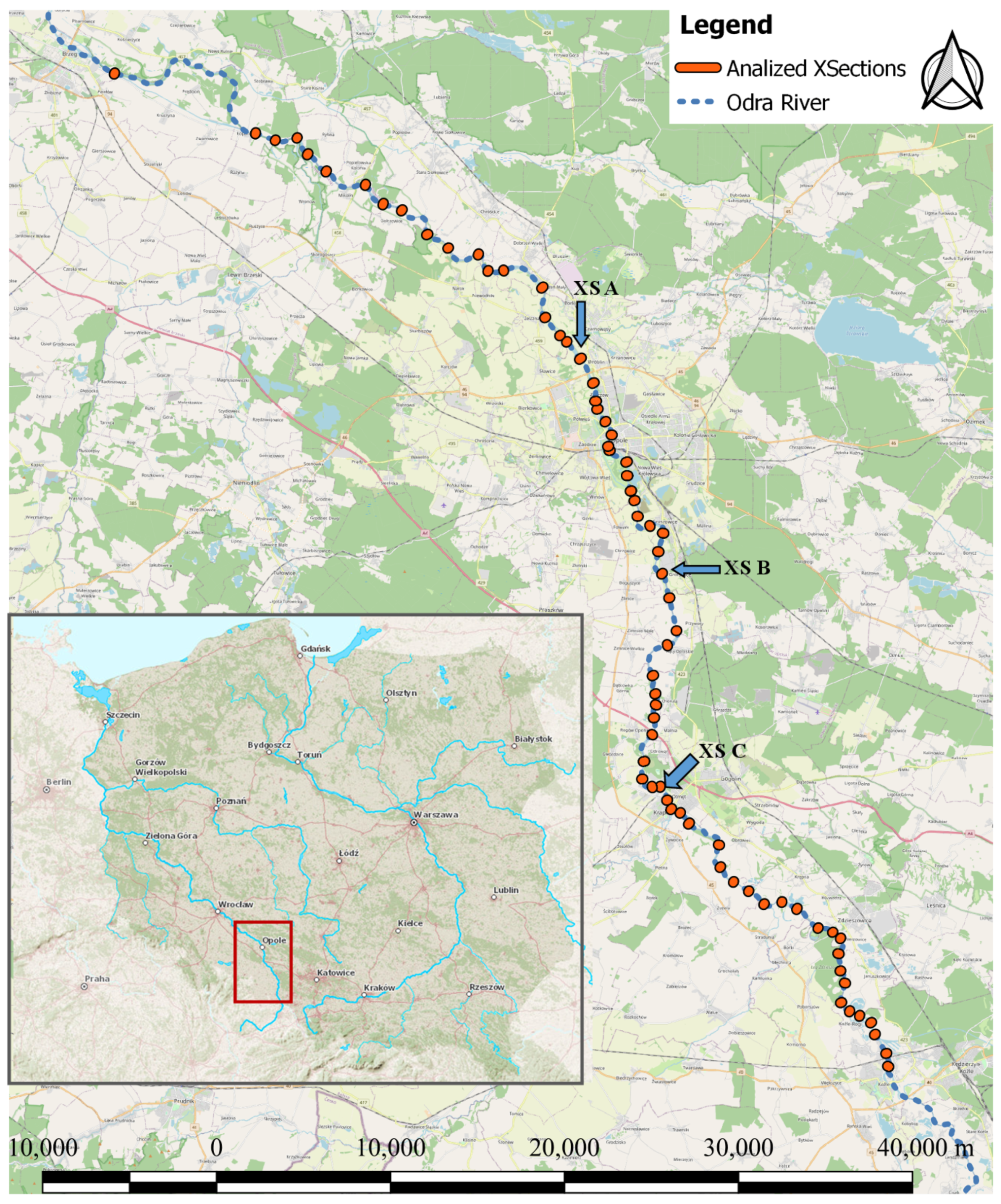
• The Upper Odra: From the source in Czequia of the river up to the city of Kędzierzyn-Koźle with a total length of 202 km;
• The Middle Odra: From Kędzierzyn-Koźle, up to the discharge of the river Warta (the main tributary of the Odra) with a total length of 522 km;
• The Lower Odra: from the river Warta up to the Dąbie lake with a length of around 130 km.

The actual Odra River along its canalized part is located in the southern part of Poland (within the Middle Odra subbasin) and is classified as a waterway of regional importance. Twenty-five low head barrages compose this part of the Odra River (the Odra Cascade) [23].

According to the legislation for the operation of inland waterways, the minimal and maximal operational [24] shall be established on the basis of two operational flow rates, namely, Q${}_{276}$ and Q${}_{14}$, respectively. The subscript 276 represents the number of days in a year that the water flowing along the Odra is higher than Q${}_{276}$ (minimal operational value) and the subscript 14 represents the number of days in a year that the water flowing along the Odra is lower than Q${}_{14}$ (maximal operational value). Within the analyzed reach (the Odra Cascade), the values of Q${}_{276}$ vary from 21.1 [m${}^3$ s${}^{-1}$] to 64.5 [m${}^3$ s${}^{-1}$], while for Q${}_{14}$, its values vary from 233 [m${}^3$ s${}^{-1}$] to 459 [m${}^3$ s${}^{-1}$] [24].

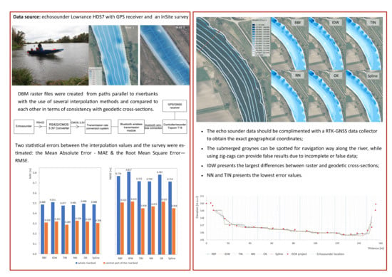
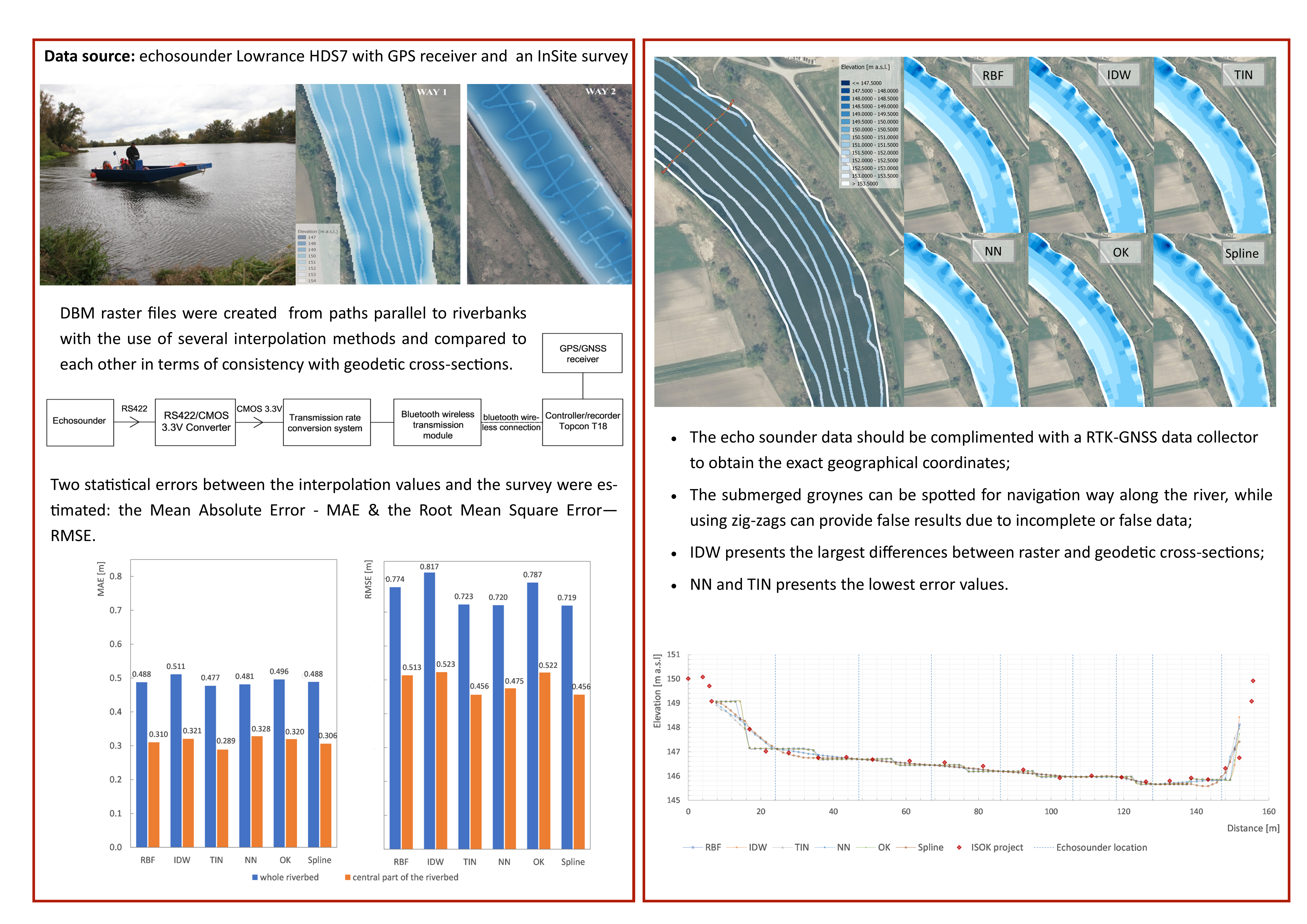
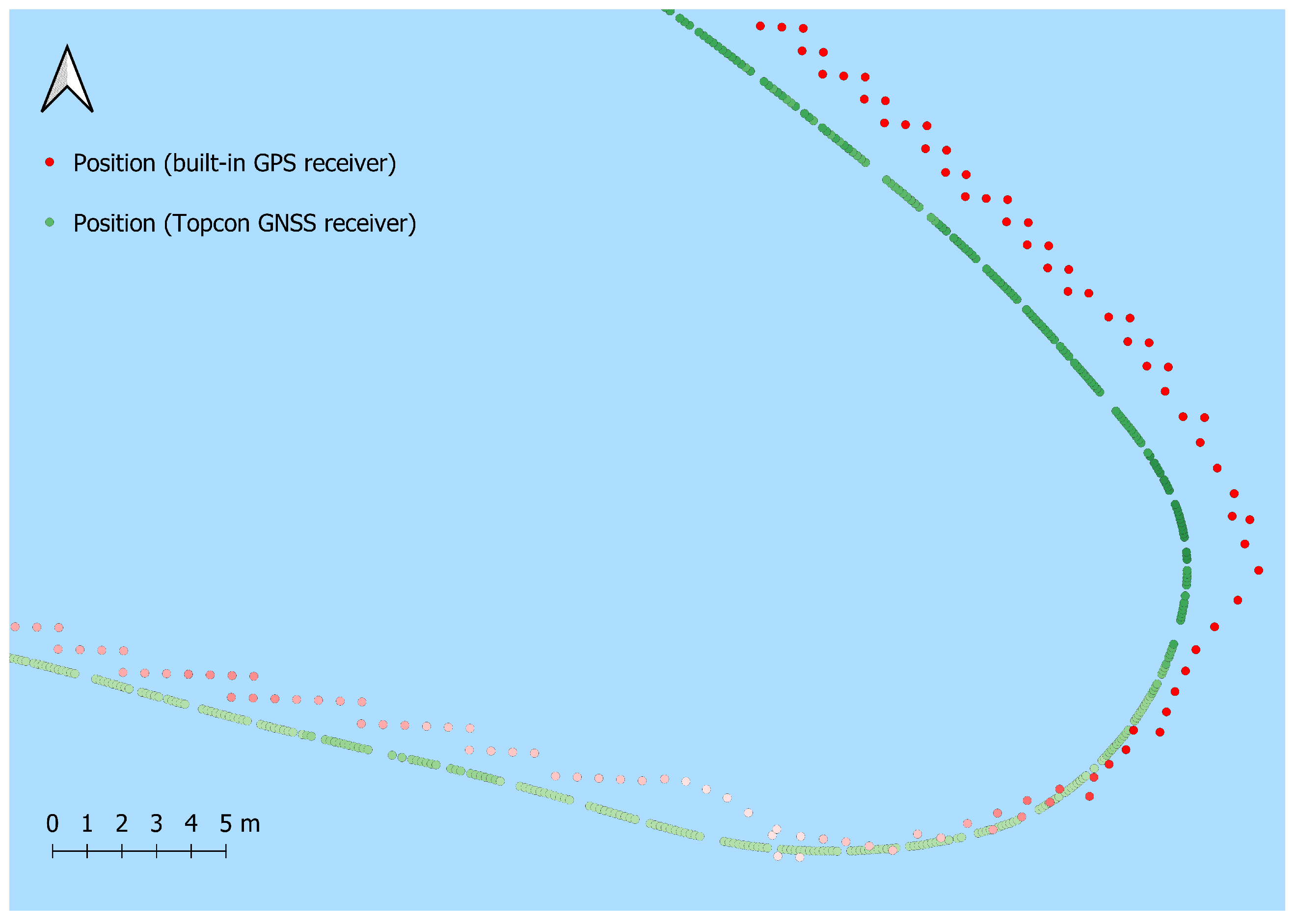
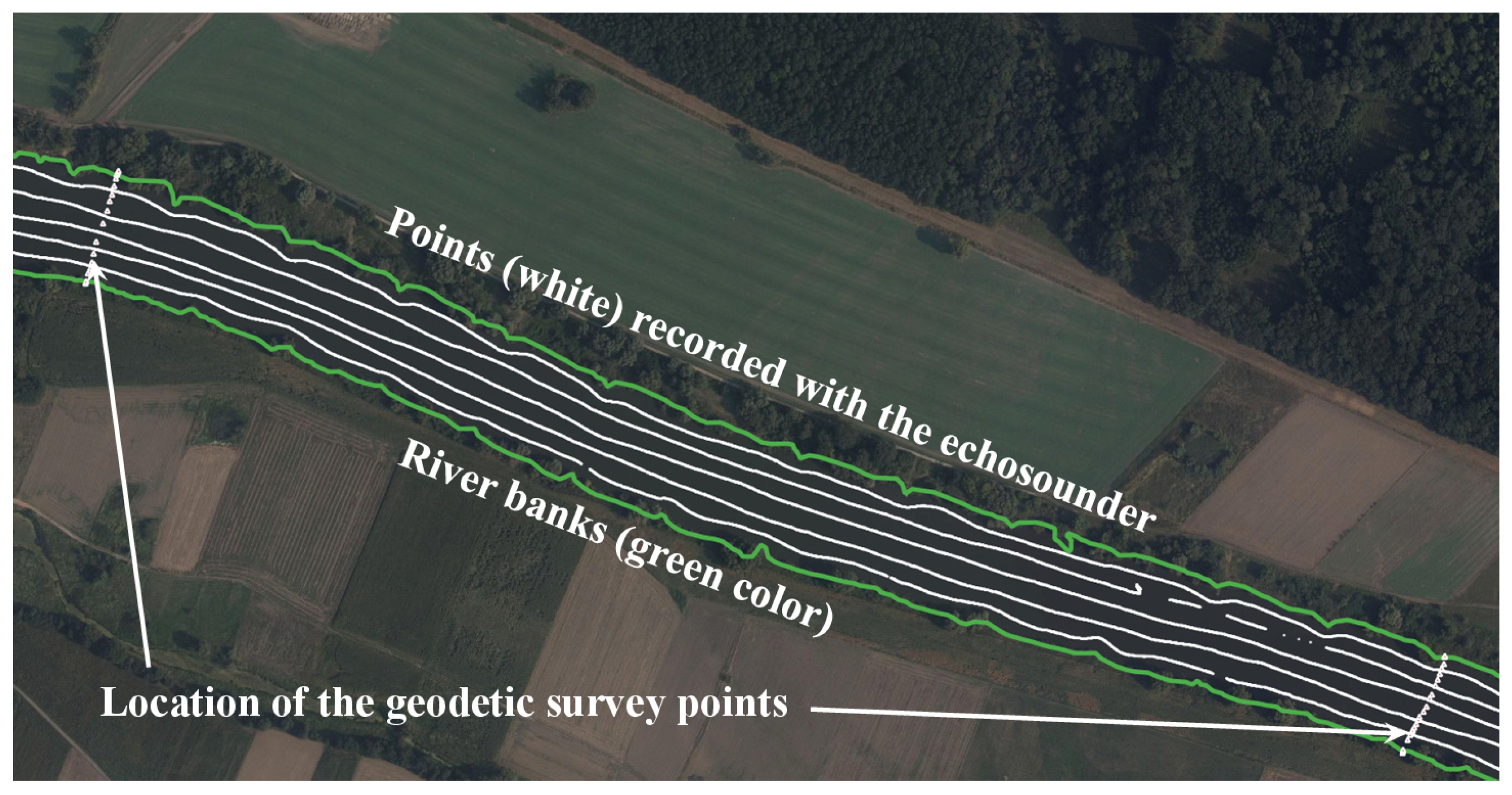
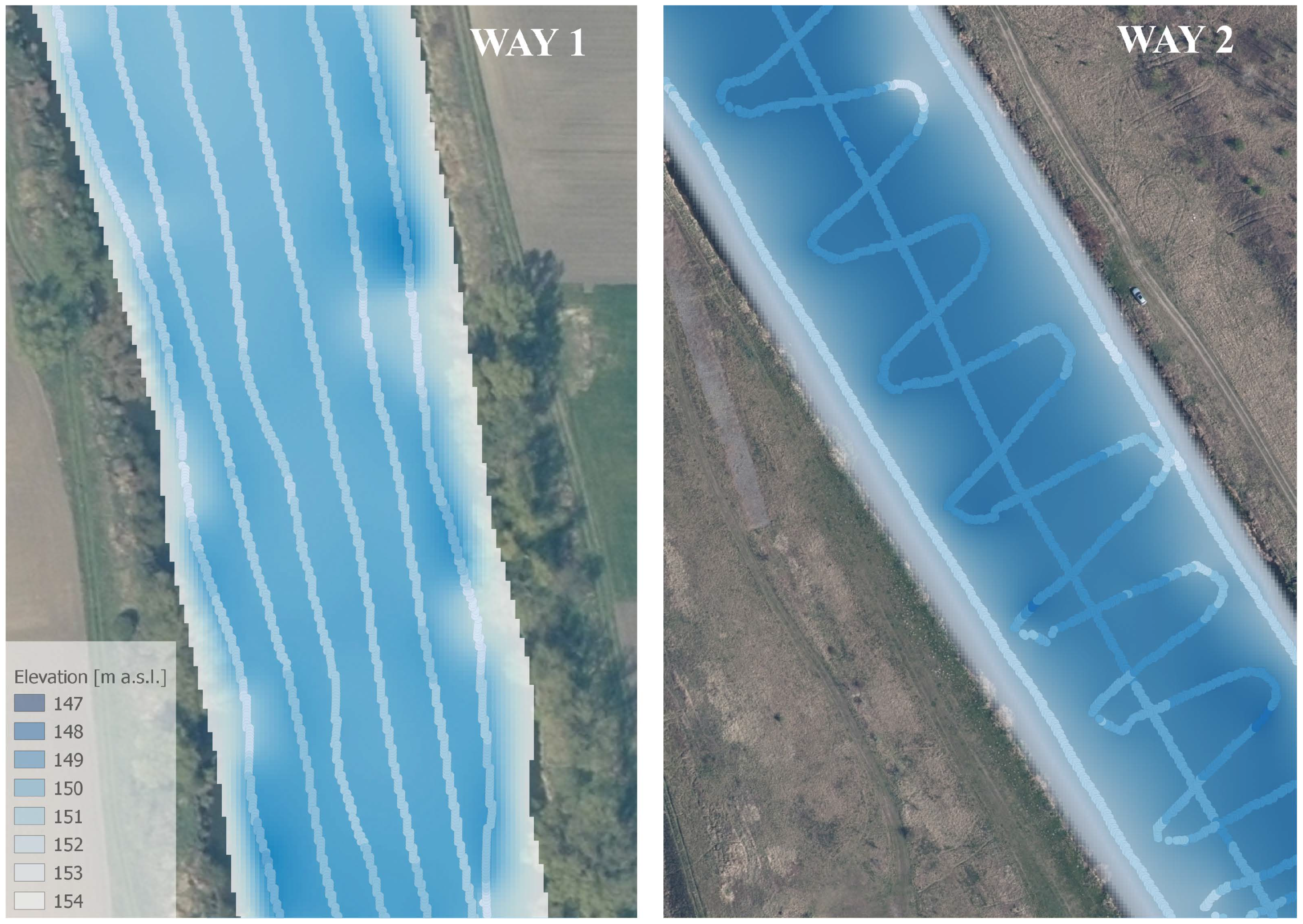
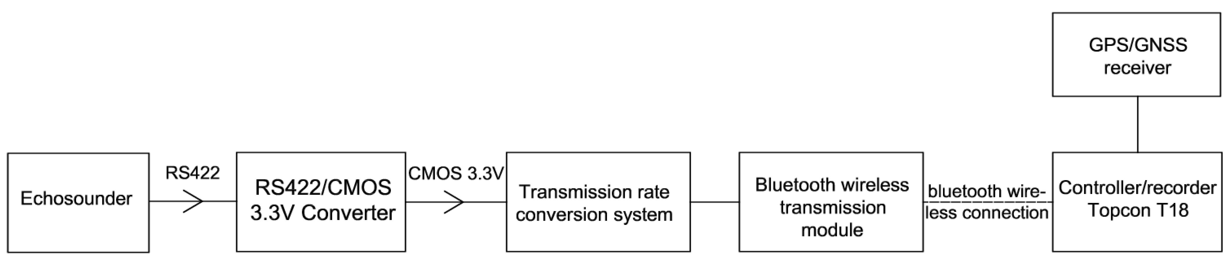
2.1. Surveying and Data Collection

The data used for this research were obtained from the bathymetric survey on the Odra river [1]. The point data were collected using an acoustic sonar together with an integrated GPS receiver, which enabled obtaining the location of the surveyed points of the riverbed; nonetheless, the geographical location of the surveyed points was corrected with the integration of a Topcon GNSS with the echo sounder during the survey.

The used equipment (Lowrance HDS) employs CHIRP (Compressed High Intensity Radar Pulse), which is an improved version of sonar technology, using a combination of different ultrasound frequencies instead of one. It enables spotting objects of various consistency, responding to different sonar frequencies and improves bottom tracking as adjacent objects are separated. Typical CHIRP frequencies are 28/51 kHz (Low), 85/155 kHz (Medium), or 140/250 kHz (High). During the survey, we used med/high CHIRP frequency, which is appropriate for shallow water.

The correction of the geographical points thanks to the mentioned HDS7-GNSS connection is observable and depicted in Figure 1. The red dots display the geographical location obtained from the GPS receiver of the HDS7 while the green dots depict the geographical location from the Topcon GNSS. GNSS receiver enabled the correction of the water table, which varies along and across [25] the river. This equipment was installed in a small motorboat, which allowed collecting data even in shallow waters (with a minimal 1 m water depth) near to the riverbanks [26].

The survey was also conducted along several paths parallel to the riverbanks at an interval of around 10 to 20 m depending on the total width of the river. Figure 2 depicts some typical routes (white lines parallel to the river path) that were used for collecting data (with the purpose of building the DiBMs) showing the geodetic survey points (perpendicular white dash lines of Figure 2) that were carried out previously within the framework of the ISOK project. The river bank lines (depicted in green in Figure 2) were also defined on the basis of the previously mentioned ISOK project.

Figure 3 depicts the location of the cross-sections (orange) that were analyzed (around seventy in total, from which forty were selected, where the river bed did not show significant differences from the time of the geodetic survey and the time of the data collection due to natural hydromorphological changes) in this contribution along the canalized part of the Odra River and their geographical location in Poland.

As depicted in Figure 4, two navigation schemes were tested for data collection to carry out the survey in shorter periods of time. One main problem was identified: The boat inclination during the turns where the riverbed is shallow can provide larger or shorter water depth values, so the boat turn shall be very slow, or the obtained data must be deleted. The two ways of navigation consume a similar amount of time. For surveying river reaches of around 8 km length, at least 6–7 h were necessary. Way 1 (parallel lines along the river path) results in less error and submerged groynes can be spotted. Way 2 (3 parallel paths and one “zig-zag” path), results in false results (larger “white spots”) because of lack of data.

As it was shown in Figure 4, the most problematic area with the largest values of error is the part of the riverbed, where it is shallow (near the banks). Using way 2, data from these points are not as reliable as data from navigation way 1. Moreover, at least 2 paths parallel to the banks (closest to the bank as possible) were needed to collect data without errors caused by the tilt of the turn. Since on the central part of riverbed the data error values are small, in the case of long river sections, navigation only along the river is sufficient, as the perpendicular path consumes a lot of time—which can be better used by increasing the number of paths along the river and careful navigation as close to the bank as possible. For this contribution, way 1 of navigation was used for the survey and analysis of interpolation methods is carried out for this configuration.

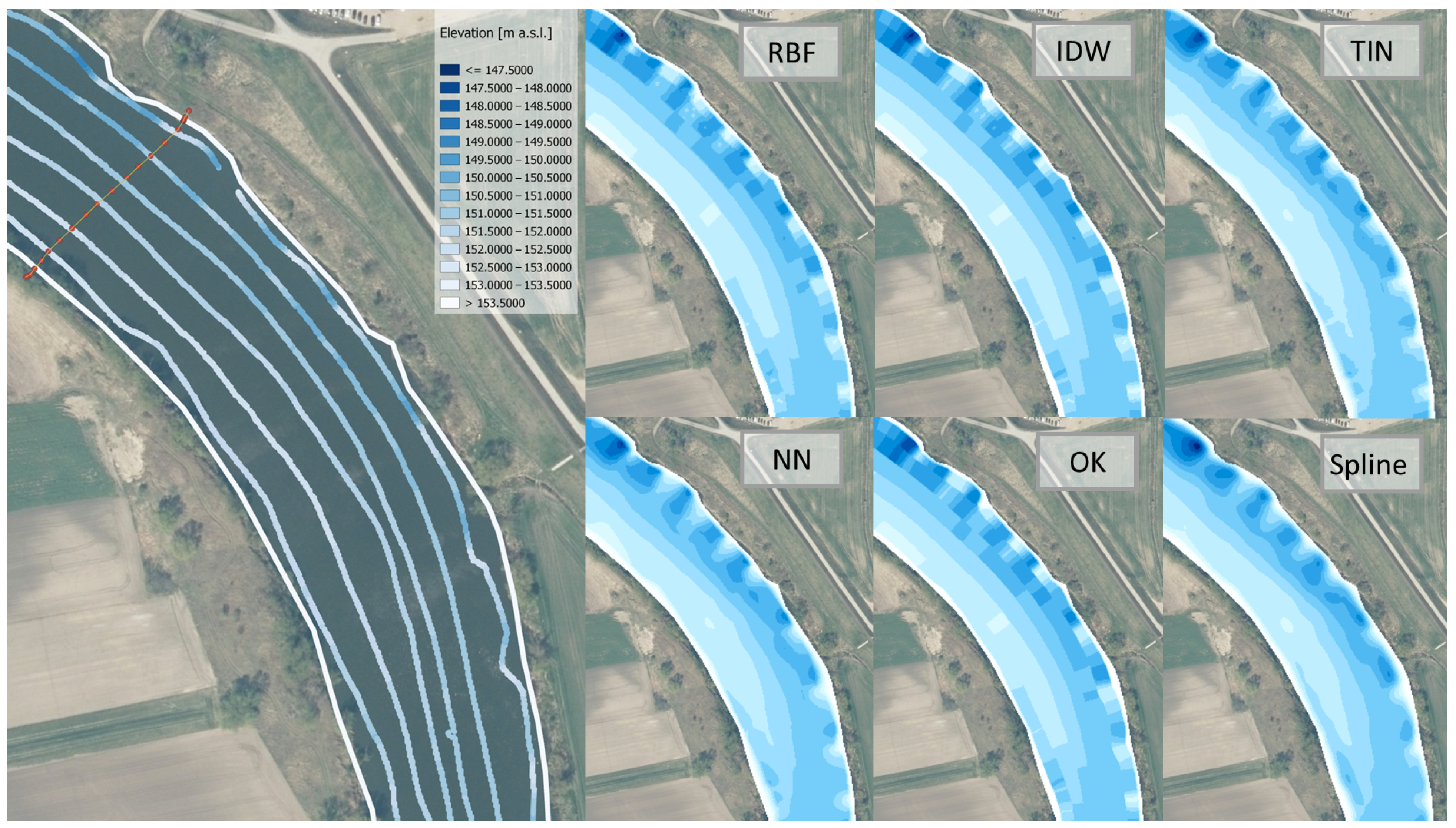
2.2. Data Processing and Interpolation Methods

To obtain the exact position and elevation of the riverbed data points, the depth data from the echo sounder have to be collected together with its precise location. As fish finders are equipment, which do not pair with RTK (Real Time Kinematic)-GPS, to obtain the connection that allows the precise position recording, first depth data in NMEA0183-compliant format have been transmitted from the transducer through a built-in RS422 port. To match the requirements of the Topcon T18 controller, the data has been then converted to CMOS 3.3V signal and transmitted at the rate acceptable by the controller via Bluetooth. Finally, the combined data from the echo sounder and GPS/GNSS receiver was recorded on a memory card by the Topcon controller. The connection scheme describing this procedure is depicted in Figure 5.

The set of data points in format (x, y, elevation) for one path (usually 6–10 km long) has been recorded as one file (sl2). Files for one reach between the barrages were collected and complemented with the riverbanks location, obtained from the ISOK information. Once the data were processed, the DiBMs were created using mainly three programs, namely, reefmaster, QGIS, and ArcGIS. After a GIS database of paths containing the surveying points was built, the next step was to carry out the interpolation procedure for the raster map creation. Spatial interpolation methods are generally divided between deterministic and statistical methods. Among the popular deterministic methods are TIN, IDW, NN, Spline, and RBF. Statistical methods are based on the Kriging method.

After preliminary tests [26], the following methods were compared in terms of usefulness for riverbed bathymetry:

• TIN: this method where a Triangulated Irregular Network is created with the use of the Delaunay Triangulation procedure and the values are calculated from three vertices of a given triangle;
• Spline: this method uses functions minimizing the overall surface curvature and yields a smooth surface. Paramasivam & Venkatramanan [27] recommend using this method for gently varying surfaces, such as elevation, water table height, or pollution;
• IDW: it is considered as the simplest interpolation method [27]. Its interpolated value is a weighted average of point values in the neighborhood with inverse distance as weight;
• Multiquadric RBF: it is a group of deterministic methods, giving a smooth surface passing through the data points, with the possibility of obtaining values that are out of the measured range;
• NN: it is a method of interpolation based on Voronoi polygons—only neighboring polygons contribute to the interpolated value, with the weight depending of cut area;
• Kriging: it is a family geostatistical methods, where weights depend on the spatial correlation between the datapoints, described by the semivariogram. The method used for this contribution is the ordinary Kriging (OK), assuming an unknown, but constant mean.

According to the cited papers [3,20,21,22], it is unclear how to determine which method is the best to prepare a proper DEM of river bathymetry in the case of parallel navigation (surveying). On the one hand, popular methods such as IDW and Kriging seem to be preferred by most researchers [15,19,20,21]. On the other hand, some researchers suggest TIN or NN [3,12]. Another criterion for choosing a method of interpolation should also be the performance during merging with DEM to create a proper geometry for numerical modeling purposes. In this contribution, different interpolation (deterministic and stochastic) methods were assessed to build the bathymetry of fourteen reaches of the channelized part of the river Odra in South Poland, which represents a case study for river bed mapping of a shallow river.

The following software were used for building the database and postprocessing:

• Reefmaster: a commercial GIS software dedicated for Lowrance fish finders. Being easy to use enables raster creation with TIN interpolation with Gaussian smoothing and enables the correction of the distance between the GPS antenna and the position of the echo sounder. The smoothing option can be minimized, but not turned off, therefore the peak values are lost. It enables the export of data points [28];
• SonarViewer: free software which enables reading the .slg and .sl2 files from the HDS7 echo sounder and data export for further processing;
• ArcGIS/QGIS: these programs were used for the creation of rasters (DBM).

3. Results

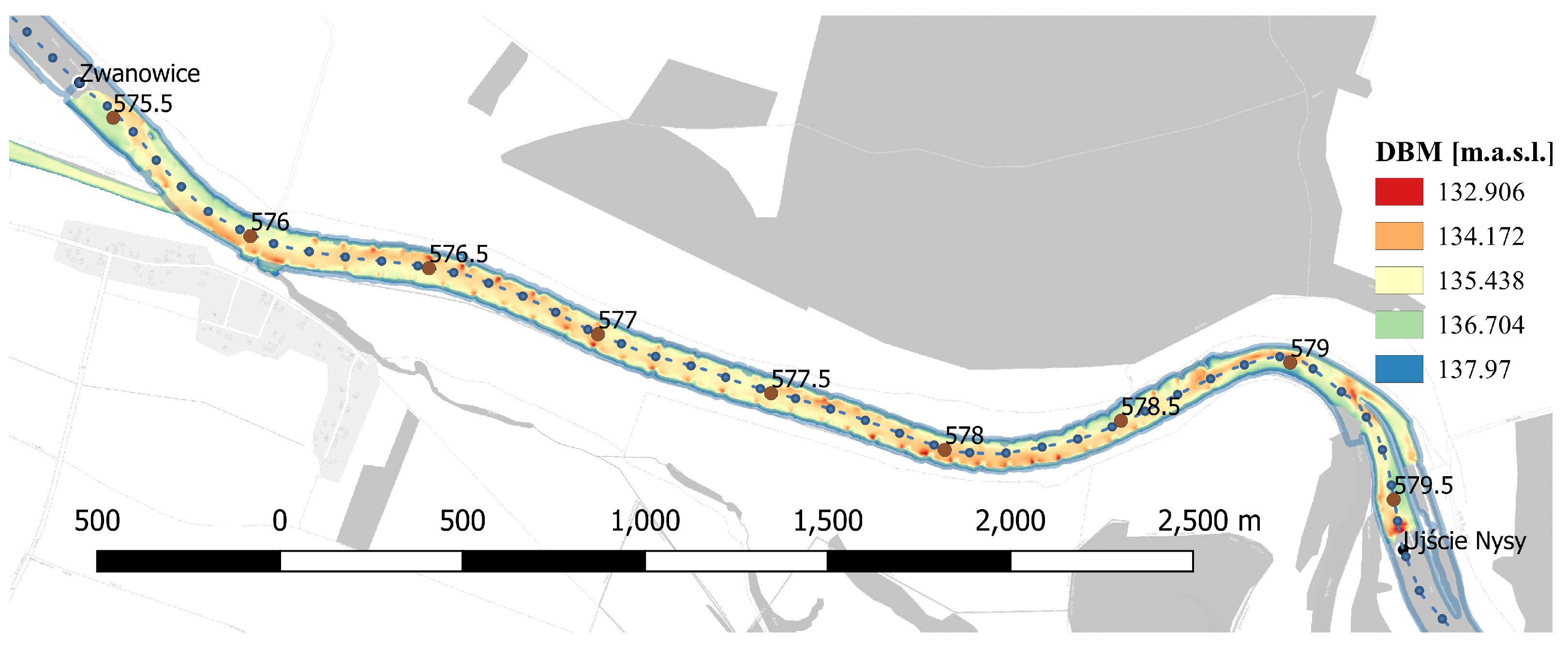
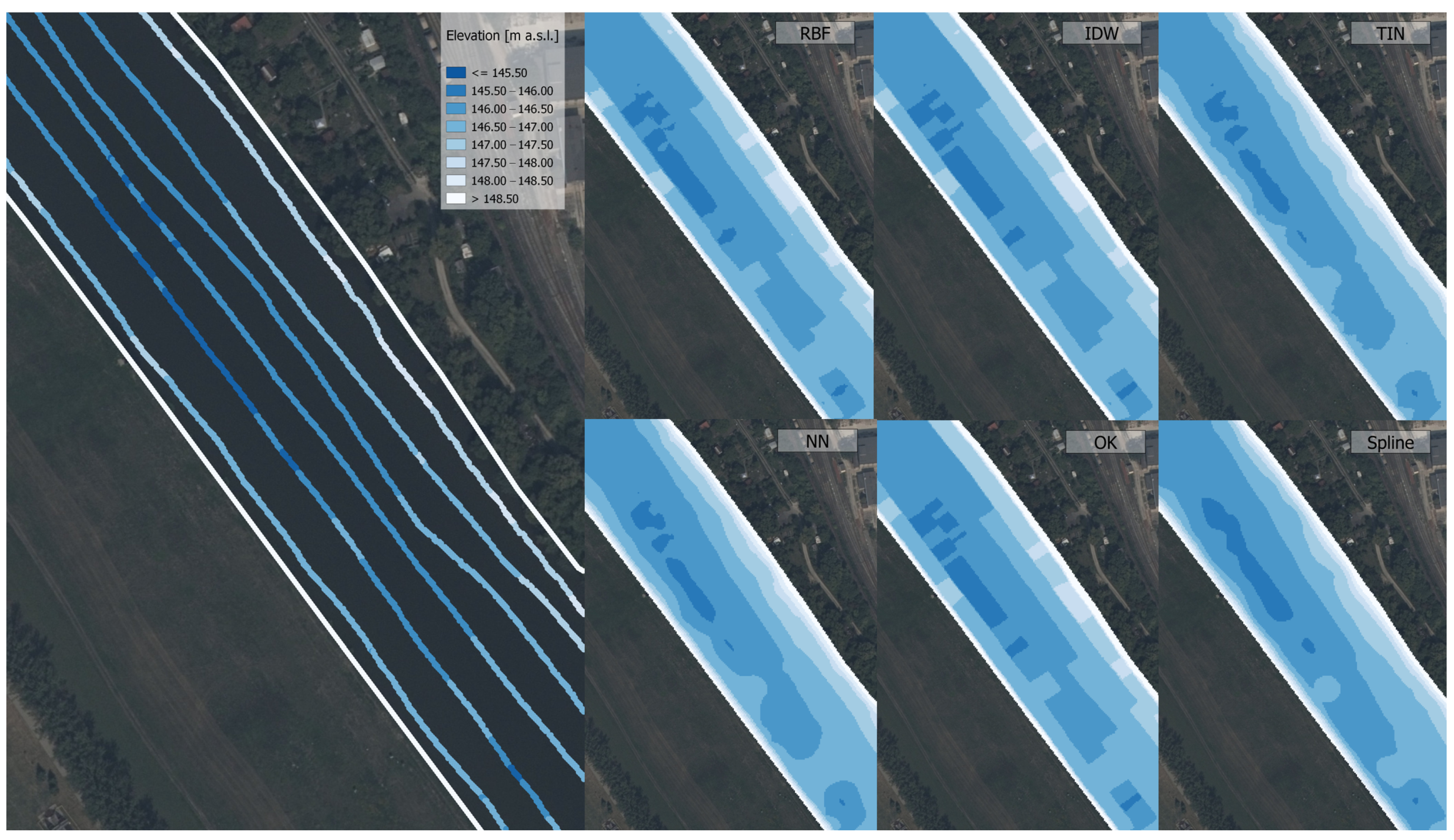
3.1. River Bed Mapping

In Figure 6, the DiBM of the reach from the barrage “Ujście Nysy” to the Barrage “Zwanowice” is depicted. This RBM was created using the interpolation method within the software Reefmaster for data acquisition from Lowrance echo sounders.

For this contribution, six interpolation methods were used for the comparison of the RBM/DiBM generation along the Odra Cascade, namely: RBF, IDW, TIN, NN, OK, and Spline. In Figure 7, the generation of six different bathymetric models is depicted for a short nonstraight reach, while in Figure 8, the DiBMs are depicted for a straight reach.

In the next section, the data of several cross-sections derived from the DiBMs and the onsite geodetic surveyed data are compared.

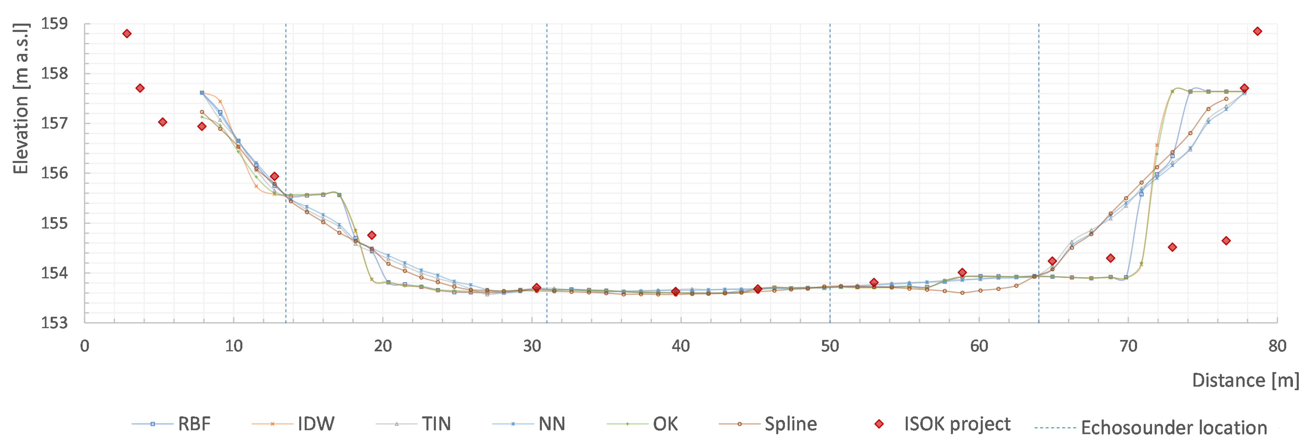
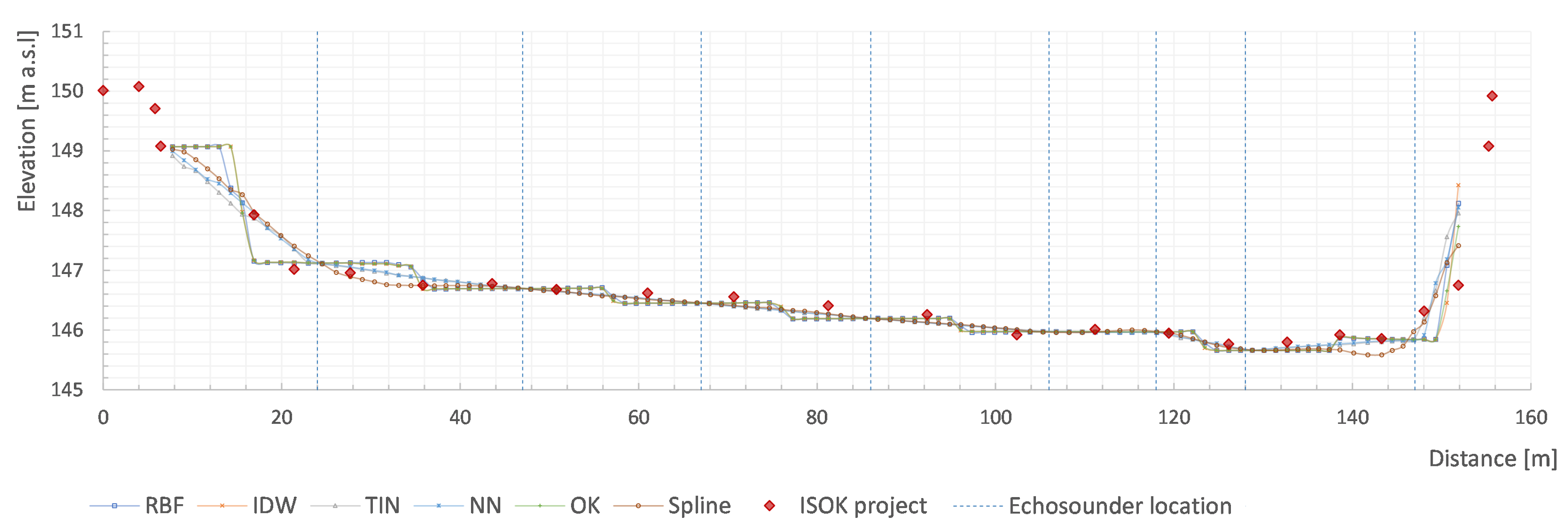
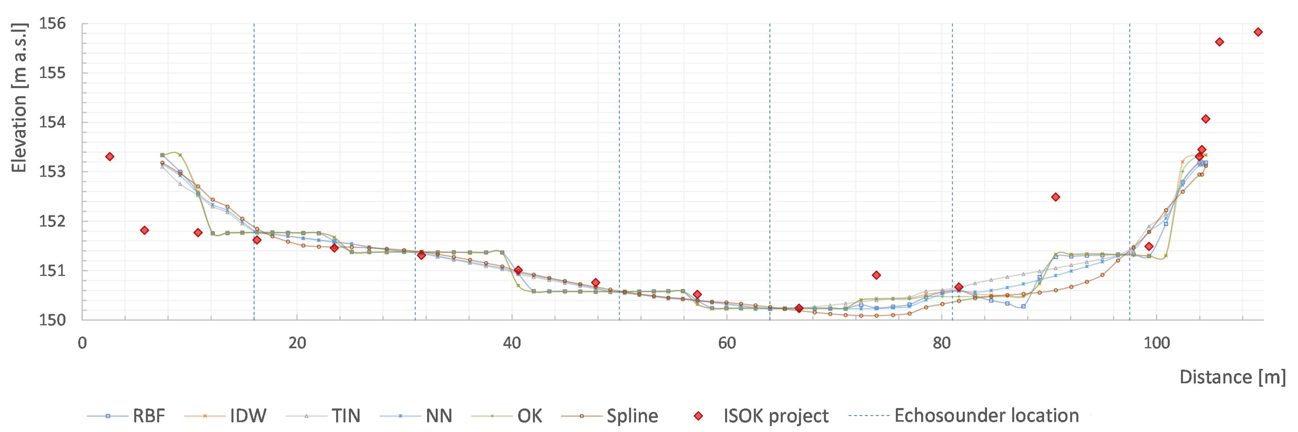
3.2. Comparison of Cross Section Data

Below, some typical cross-sections are presented, with the identification of accuracy issues. The location of the presented charts is displayed in Figure 3. The different methods are displayed using continuous colored lines, while the information from the geodetic survey (ISOK data) is depicted with a red bold diamond. The dashed blue lines represent the axis of the boat (survey lines) where the data were collected with the echo sounder. For the interpretation of the results, the first survey line is located closest to the left river bank.

As observable in cross-section C (Figure 9, chainage 125 + 200), although the data points obtained from the echo sounder fit the ISOK data in the zones near to the river banks, where the navigation possibility was constrained, it is possible to observe large discrepancies (a similar problem was pointed out by Arseni et al. [22]). The interpolated profile is smooth when the NN, TIN, or Spline method was used, while the RBF, OK, and IDW methods generated steep profiles. Large gaps between the values obtained in the central part of the riverbed are less problematical than those obtained close to the river banks.

As observable in cross-section B (Figure 10, chainage 141 + 500), apart from a discrepancy near to the left riverbank, there is a large error between the 5th and and 6th survey lines, and a smaller between 4th and 5th lines (in this case, those lines fit almost perfectly the ISOK data). Such events are hard to be forecast by any interpolation method as they are unexpected. The only proposed solution is to add more data points/survey lines that would help to resolve this issue. Nonetheless, even with additional data points, still some uncertainty may occur.

As observable in cross-section A (Figure 11, chainage 157 + 020), the survey lines were dense (more data collection); on the right side there was the possibility to navigate near to the bank (no groynes), so the interpolated riverbed profile of this part is exceptionally well shaped. Moreover, one can observe the differences resulting from the methods of interpolation; apart from the differences between the steep profile of the RBF/IDW/OK methods and the smooth shapes of the NN/Spline/TIN methods (previously described); in the zone of deflection, the spline method reaches unrealistic minimum values.

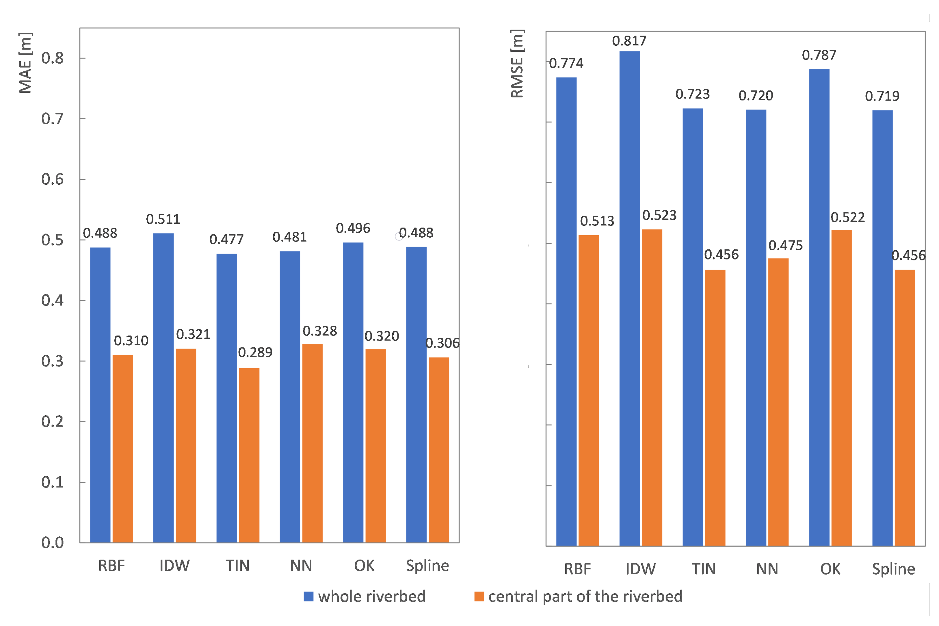
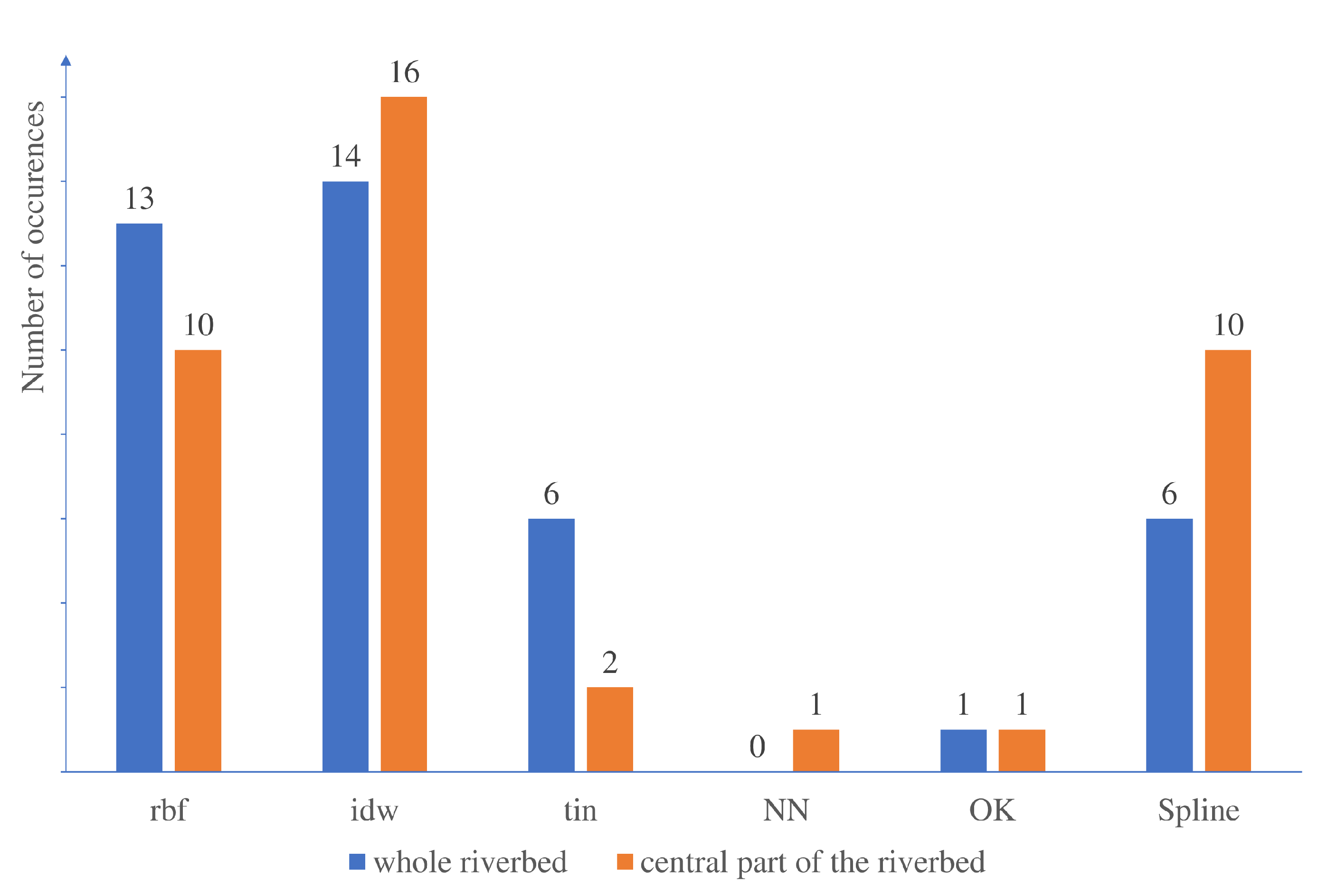
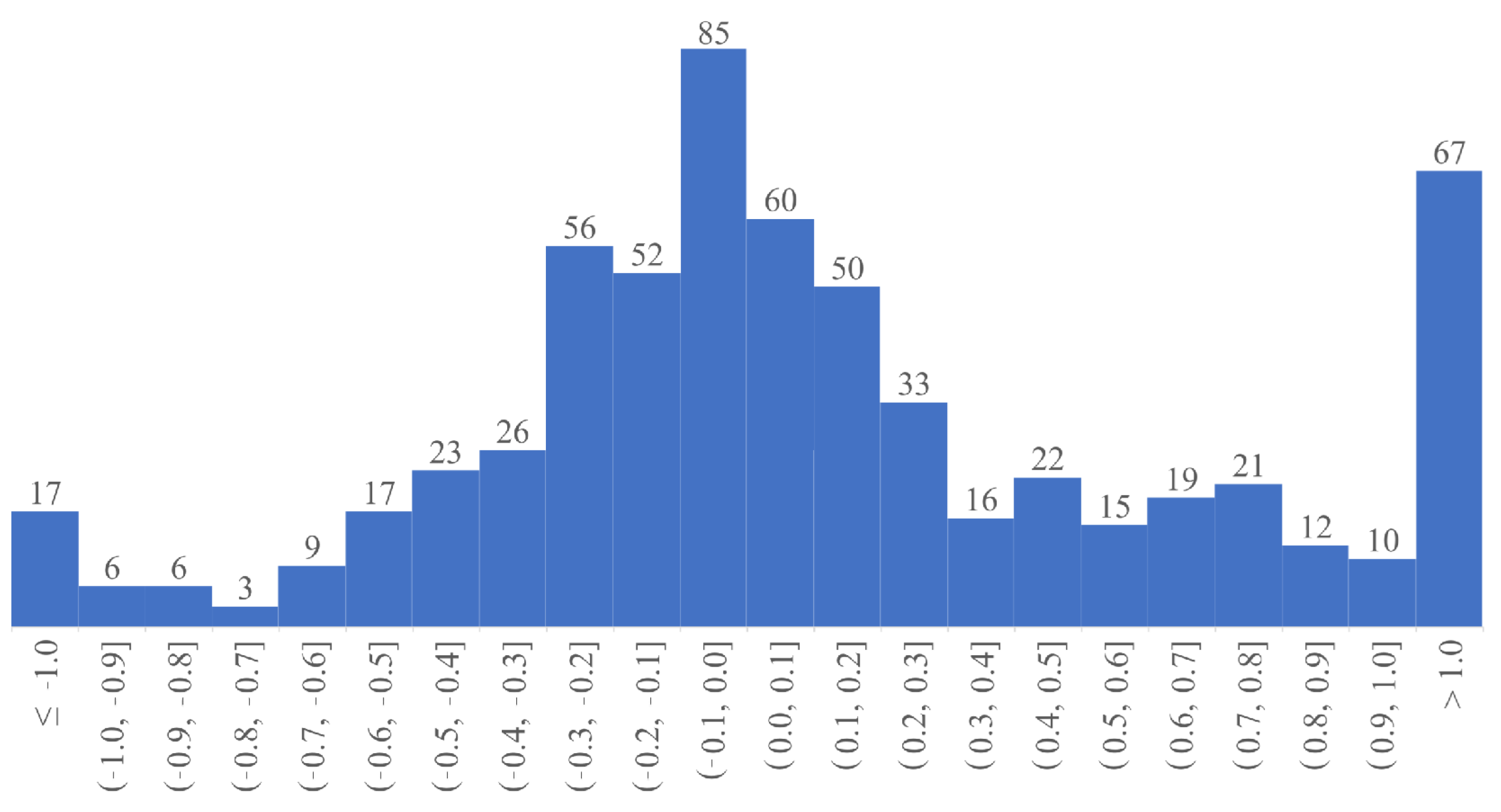
3.3. Analysis of Statistical Errors

Forty cross-sections (611 survey points) were analyzed in terms of the difference between the obtained values from ISOK and the values from the interpolation procedure. These cross-sections were selected on the basis of the identified sections with a more developed armored bed layer [29] to guaranty the reliability of the comparison. The difference between these two values we call later in this text “error”.

The mean error (ME) was calculated for all analyzed data points. This measure can provide useful information as it can consider the direction of the errors. However, the results must be interpreted carefully, as the error values with different signs can cancel out themselves. The MAE is defined as

$$\mathrm{MAE}=\frac{1}{n}\sum _{i=1}^n\left|z{i}_i-z{s}_i\right|$$

(1)

where n is a number of points, $zi$ is the value obtained from interpolation, and $zs$ is the value obtained from the geodetic survey, is a popular error measure. It does not consider the direction of errors, given their average magnitude. In this method, all errors have equal weight. Furthermore, the Root Mean Square Error (RMSE) was calculated.

$$\mathrm{RMSE}=\sqrt{\frac{1}{n}\sum _{i=1}^n{\left(z{i}_i-z{s}_i\right)}^2}$$

(2)

RMSE is another popular error measure giving an absolute value, but due to squaring of errors, it gives higher weight to larger errors. RMSE is always larger than or equal to the MAE (RMSE = MAE, when all errors have the same magnitude); the greater the difference between RMSE and MAE, the greater the variance of errors.

As an additional indicator for finding the most proper method of interpolation, for every method in every cross-section, a point with the maximum error value was found, and the method resulting with the highest error value in the given cross-section was identified. Then, the occurrences of the maximum error value in cross-section were summed up, resulting in the number of occurrences of the maximal error value in all analyzed cross-sections.

The comparisons of the errors are summarized in

Table 1. Summary of the statistical parameters for the six interpolation methods.

	dim	RBF	IDW	TIN	NN	OK	Spline
Whole Cross-Section
RMSE	[m]	0.774	0.817	0.723	0.720	0.787	0.719
MAE	[m]	0.488	0.511	0.477	0.481	0.496	0.488
ME	[m]	0.173	0.187	0.160	0.165	0.170	0.126
Median	[m]	0.012	0.031	0.039	0.049	0.030	−0.006
#Max	[-]	13	14	6	0	1	6
Central Part of Riverbed
RMSE	[m]	0.513	0.523	0.456	0.475	0.522	0.456
MAE	[m]	0.310	0.321	0.289	0.328	0.320	0.306
ME	[m]	0.041	0.047	0.043	0.041	0.045	-0.022
Median	[m]	−0.027	−0.026	−0.029	−0.028	−0.027	−0.076
#Max	[-]	10	16	2	1	1	10

and compared in Figure 12 and Figure 13.

In Figure 12, one can compare MAE and RMSE values for the whole riverbed, including areas near to the banks in the middle section of the riverbed.

Maximum error values were identified for every cross-section. Both for the whole riverbed and its central part, the maximum errors occurred most frequently for the IDW interpolation method. As can be observable from the results of Figure 12 and Figure 13, the least frequency of maximum error in the cross-section is given by the NN and OK methods.

The histogram of error is shown in Figure 14—the difference between histograms is small, so the histogram for the TIN method was chosen as the example.

4. Discussion

The largest values of errors can be observed in the parts of the riverbed by the banks—they can be minimized by careful navigation near to the banks (right bank on the Figure 11), but it is not always possible, due to groynes and submerged objects in this area.

Santillan et al. [30] stated that the parallel method of navigation gives less accurate results than cross-sections and zig-zags, but their results concern a wide reservoir (not a shallow river) and the dataset contains only three paths (and less data points than the other compared methods). Of course, a set of orthogonal cross-sections as dense as parallel lines would improve the accuracy of the interpolation, but such method of navigation may consume a lot of time and it is inconvenient for surveying long river reaches. This conclusion is compatible with the statement of Kruger et al. [16] that one must choose a strategy based not only on the accuracy, but also on the workload and costs.

Since the errors are large for all methods, RMSE and MAE were calculated also for the central part of the riverbed—the error values were smaller (Table 1) but still significant—from the comparison of RMSE/MAE can be seen, that although the values are smaller, large errors still play a big role; however, we should remember that the ISOK survey was carried out a few years earlier (2012) [31], so there could be changes in the riverbed (cross-sections, where data about dredging were available, were not analyzed, but during this time, natural changes could also occur due to sediment transport). Another source of error was the fact that the distance between the paths was up to 20m, and some of the morphological details could be omitted (Figure 10). The differences resulting from the interpolation method are 13–15% of RMSE and 12–13% of MAE for the central part of the riverbed.

From the cross-sections (Figure 9, Figure 10 and Figure 11) and the values of Table 1, it is possible to notice that the methods that are producing rough surfaces (caused by the dataset composed of clustered points [32]), such IDW, OK, and RBF, also give larger values of mean errors: RMSE 0.513–0.522 m and MAE 0.310–0.321 m. The second group of methods, producing smooth surfaces (TIN, NN, and Spline) perform better: RMSE 0.456–0.475 m and MAE 0.289–328 m (for the central part of riverbed). The compared methods of interpolation vary significantly in zones near the river banks giving maximum values of error in these locations. From the charts of Figure 12 and Figure 13, one can observe that both RMSE and MAE values for the whole riverbed are 1.5 to 1.6 times larger than those for the central part of the river. This fact is because of large errors in the data collection near to the banks, where the boat could not navigate due to the rapidly decreasing depth (in many cases because of the presence of groynes). This part of the riverbed is the most problematic for the bathymetry map creation.

For all interpolation methods, the mean error values are positive, but the median values are close to zero. The mean values are affected by the outliers on the positive error side; this is confirmed by the histogram of Figure 14, from which we can observe that most of the error values concentrate near to the 0 value and the number of positive and negative errors is similar but there are slightly more negative errors—that could result from the method accuracy and/or the fact, that the surveys were not carried out at the same time. However, the values of negative errors are usually small, while there are a lot of outliers on the positive side (parts of the riverbed near to the banks).

Most of the cited research was focused on the comparison of methods such Kriging, IDW, and RBF [15,19,20,21]. These methods perform in a similar way, creating rough surfaces. The authors can agree with [15,21] that the Kriging method performs slightly better than IDW. However, more interesting seem to be the results derived from the NN and spline methods, which created a smooth surface (more realistic as the bottom surface), as was noticed by Bio et al. [3], which merges better with DEM. Furthermore, as smooth surfaces, these methods do not need smoothing procedures for isoline creation. These methods also have slightly lower error values than IDW or OK. For the NN method, the maximum value of error was never estimated along the cross-sections, and in general the $RMSE$ values for these methods (NN and Spline) are lower than these obtained for the IDW/OK/RBF methods. The main disadvantage of the Spline method is the fact that it gives unrealistic minimum values in the inflection area. In terms of $MAE$, the best performing method is TIN (it also performs nearly as well as spline/NN in terms of $RMSE$). The TIN method, although it is very simple, performs remarkably well in terms of errors both for the cross-section and the middle part of the riverbed, preserving the original values. After smoothing, the data are flattened, but the performance in terms of errors is still very good and allows for realistic RBM creation.

5. Conclusions

As described in the Section “Materials and Methods”, during the survey of the present study, a fish finder echosounder with a med/high CHIRP frequency was used. According to Horta et al. [33], the accuracy of such kind of instrumentation is around 1 mm. Nonetheless, the accuracy of the measurements depends on several factors such as the velocity of the boat during the survey, bottom composition, or water cleanliness [11] resulting that the accuracy of the measurements was 100 times smaller than the accuracy of the instrumentation. However, with the implementation of proper corrections during the survey, the error can be reduced and the instrumentation is reliable for the creation of RBM.

Using a single-beam echo sounder for large-scale bathymetry survey can be a fast, economical, and reliable method after some improvements, e.g., the built-in GPS receiver is useless for determining the elevation and significantly imprecise in determining the geographical coordinates. Therefore, the echo sounder data should be complimented with a RTK-GNSS data collector to obtain the exact geographical coordinates. Another issue is the choice of the navigation scheme (way) when the time or budget is limited; longitudinal (parallel to the water path) navigation along the river performs sufficiently well as additional cross-sections (zig-zags) are time-demanding and impractical, especially for a narrow river such as the Odra. Apart from depth in the central part of the river, an important issue is the spotting of submerged groynes as it was depicted in Figure 4. The submerged groynes can be spotted for navigation way along the river (way 1), while using zig-zags can provide false results due to incomplete or false data.

References

1. Kostecki, S.; Machajski, J.; Herrera-Granados, O.; Uciechowska-Grakowicz, A.K.; Maniecki, Ł.; Sawicki, E. Project on the Enhancement of the Navigability of the Odra River. Reports and Recomendations. Part 1A; Tech. Reports of the Faculty of Civil Engineering; Wrocław University of Science and Technology: Wrocław, Poland, 2019. (In Polish) [Google Scholar]
2. Yamasaki, S.; Tabusa, T.; Iwasaki, S.; Hiramatsu, M. Acoustic water bottom investigation with a remotely operated watercraft survey system. Prog. Earth Planet. Sci. 2017, 4, 25. [Google Scholar] [CrossRef] [Green Version]
3. Bio, A.; Gonçalves, J.A.; Magalhães, A.; Pinheiro, J.; Bastos, L. Combining Low-Cost Sonar and High-Precision Global Navigation Satellite System for Shallow Water Bathymetry. Estuaries Coasts 2020. [Google Scholar] [CrossRef]
4. Okabe, T.; Kato, S. Temporal changes in the ebb-tidal delta bathymetry of Imagire-guchi inlet in Japan. Coast. Eng. J. 2018, 60, 437–448. [Google Scholar] [CrossRef]
5. Molenda, T.; Czajka, A.; Czaja, S.; Spyt, B. Rapid River Bed Recovery after the In-Channel Mining: The Case of Vistula River, Poland. Water 2021, 13, 623. [Google Scholar] [CrossRef]
6. Pacina, J.; Lend’Áková, Z.; Štojdl, J.; Grygar, T.M.; Dolejš, M. Dynamics of sediments in reservoir inflows: A case study of the skalka and nechranice reservoirs, Czech Republic. ISPRS Int. J. Geo-Inf. 2020, 9, 258. [Google Scholar] [CrossRef] [Green Version]
7. Dumpis, J.; Lagzdiņš, A. Methodology for Bathymetric Mapping Using Open-Source Software. Environ. Clim. Technol. 2020, 24, 239–248. [Google Scholar] [CrossRef]
8. Halmai, Á; Gradwohl-Valkay, A.; Czigány, S.; Ficsor, J.; Liptay, Z.Á; Kiss, K.; Pirkhoffer, E. Applicability of a recreational-grade interferometric sonar for the bathymetric survey and monitoring of the Drava River. ISPRS Int. J. Geo-Inf. 2020, 9, 149. [Google Scholar] [CrossRef] [Green Version]
9. Madusiok, D. A bathymetric unmanned surface vessel for effective monitoring of underwater aggregate extraction from the perspective of engineering facilities protection. Arch. Min. Sci. 2019, 64, 375–384. [Google Scholar] [CrossRef]
10. Osadczuk, A. Geofizyczne metody badań osadów dennych. Stud. Limnol. Telmatologica 2007, 1, 25–32. [Google Scholar]
11. Gołuch, P.; Kaplon, J.; Dombek, A. Evaluation of data accuracy obtained from batymetric measurement using the fishfinder LOWRANCE LMS-527C DF iGPS. Arch. Fotogram. Kartogr. Teledetekcji 2010, 21, 109–118. (In Polish) [Google Scholar]
12. Milne, J.A.; Sear, D.A. Modelling river channel topography using GIS. Int. J. GIS 1997, 11, 499–519. [Google Scholar] [CrossRef]
13. Song, Y.; Huang, J.; Toorman, E.; Yang, G. Reconstruction of river topography for 3d hydrodynamic modelling using surveyed cross-sections: An improved algorithm. Water 2020, 12, 3539. [Google Scholar] [CrossRef]
14. Dysarz, T. Development of RiverBox-An ArcGIS toolbox for river bathymetry reconstruction. Water 2018, 10, 1266. [Google Scholar] [CrossRef] [Green Version]
15. Wu, C.Y.; Mossa, J.; Mao, L.; Almulla, M. Comparison of different spatial interpolation methods for historical hydrographic data of the lowermost Mississippi River. Ann. GIS 2019, 25, 133–151. [Google Scholar] [CrossRef]
16. Kruger, R.; Karrash, P.; Bernard, L. Evaluating Spatial Data Acquisition and Interpolation Strategies for River Bathymetries. In Geospatial Technologies for All; Springer: Cham, Switzerland, 2018; pp. 189–209. [Google Scholar] [CrossRef]
17. Glenn, J.; Tonina, D.; Morehead, M.D.; Fiedler, F.; Benjankar, R. Effect of transect location, transect spacing and interpolation methods on river bathymetry accuracy. Earth Surf. Process. Landforms 2016, 41, 1185–1198. [Google Scholar] [CrossRef]
18. Heritage, G.L.; Milan, D.J.; Large, A.R.G.; Fuller, I.C. Influence of survey strategy and interpolation model on DEM quality. Geomorphology 2009, 112, 334–344. [Google Scholar] [CrossRef]
19. Šiljeg, A.; Cavric, B.; Marić, I.; Barada, B. GIS modelling of bathymetric data in the construction of port terminals—An example of Vlaška channel in the Port of Ploče, Croatia. Int. J. Eng. Model. 2019, 32, 17–31. [Google Scholar]
20. Genchi, S.A.; Vitale, A.J.; Perillo, G.M.E.; Seitz, C.; Delrieux, C.A. Mapping Topobathymetry in a Shallow Tidal Environment Using Low-Cost Technology. Remote Sens. 2020, 12, 1394. [Google Scholar] [CrossRef]
21. Ferreira, I.O.; Rodrigues, D.D.; dos Santos, G.R.; Rosa, L.M.F. Em superficies batimétricas: IDW ou krigagem? Bol. Cienc. Geod. 2017, 23, 493–508. [Google Scholar] [CrossRef] [Green Version]
22. Arseni, M.; Voiculescu, M.; Georgescu, L.P.; Iticescu, C.; Rosu, A. Testing Different Interpolation Methods Based on Single Beam Echosounder River Surveying. Case Study: Siret River. ISPRS Int. J. Geo-Inf. 2019, 8, 507. [Google Scholar] [CrossRef] [Green Version]
23. Herrera-Granados, O. Numerical analysis of filling/emptying operation proposals for ship-locks chambers used for inland navigation. In River-Flow 2020, Proceedings of the of the 10th Conference on Fluvial Hydraulics, Delft, The Netherlands, 7–10 July 2020; Uijttewaal, W., Franca, M.J., Valero, D., Chavarrias, V., Arbós, C.Y., Schielen, R., Crosato, A., Eds.; CRC Press/Balkema: Delft, The Netherlands, 2020; pp. 2350–2357. [Google Scholar]
24. Dybkowska-Stefek, D. Methodology to estimate the minimum and maximum water level for inland navigation after the modernization of the Odra waterway. Biuro OdrzańSkiej Drog. Wodnej 2018. [Google Scholar]
25. Dimitriadis, P.; Tegos, A.; Oikonomou, A.; Pagana, V.; Koukouvinos, A.; Mamassis, N.; Koutsoyiannis, D.; Efstratiadis, A. Comparative evaluation of 1D and quasi-2D hydraulic models based on benchmark and real-world applications for uncertainty assessment in flood mapping. J. Hydrol. 2016, 534, 478–492. [Google Scholar] [CrossRef]
26. Uciechowska-Grakowicz, A.K.; Herrera-Granados, O. Usage of geostatistical interpolation methods for riverbed mapping and digital bathymetric modelling. In 6th IAHR Europe Congress. Book of Abstracts; Kalinowska, M., Rowiński, P., Okruszko, T., Nines, M., Eds.; PAS Publications: Warsaw, Poland, 2020. [Google Scholar]
27. Paramasivam, C.R.; Venkatramanan, S. An introduction to various spatial analysis techniques. GIS Geostat. Tech. Groundw. Sci. 2019, 20–30. [Google Scholar] [CrossRef]
28. Reefmaster. Reference Manual V2.0. 2017. Available online: https://reefmaster.com.au/reference2/index.htm (accessed on 1 December 2018).
29. Ferdowsi, B.; Ortiz, C.P.; Houssais, M.; Jerolmack, D.J. River-bed armouring as a granular segregation phenomenon. Nat. Commun. 2017, 8, 1363. [Google Scholar] [CrossRef] [PubMed]
30. Santillan, J.R.; Serviano, R.; Makinano-Santillan, J.L.; Marqueso, M. Influence of river bed elevation survey configurations and interpolation methods on the accuracy of lidar dtm-based river flow simulations. ISPRS Arch. 2016, 42, 225–235. [Google Scholar] [CrossRef] [Green Version]
31. Kostecki, S.; Machajski, J.; Banasiak, R.; Herrera-Granados, O.; Uciechowska-Grakowicz, A.K.; Maniecki, Ł; Sawicki, E. Project on the Enhancement of the Navigability of the Odra River. Reports and Recomendations. Part C; Tech. Reports of the Faculty of Civil Engineering; Wrocław University of Science and Technology: Wrocław, Poland, 2019. (In Polish) [Google Scholar]
32. Hagemen, J.; Bennett, D.A. Construction of Digital Elevation Models for Archaeological Applications. In Practical Applications of GIS for Archaeologists; Westcott, K.L., Brandon, R.J., Eds.; Taylor & Francis: Abingdon, UK, 2000. [Google Scholar]
33. Horta, J.; Pacheco, A.; Moura, D.; Ferreira, Ó. Can recreational echosounder-chartplotter systems be used to perform accurate nearshore bathymetric surveys? Ocean Dyn. 2014, 64, 1555–1567. [Google Scholar] [CrossRef]
Figure 1. Correction of the survey (red dots) points’ geographical location, obtained from the instrument GPS receiver, using the Topcon GNSS (green dots).
Remotesensing 13 04236 g001
Figure 2. Aerial view of one small river reach showing the points that were recorded with the echo sounder HDS7.
Remotesensing 13 04236 g002
Figure 3. Geographical location of the analyzed cross-sections. Source of background maps: Open Street Map and the ISOK project.
Remotesensing 13 04236 g003
Figure 4. Comparison of two navigation ways: Way 1: parallel lines and Way 2: parallel lines and zigzag.
Remotesensing 13 04236 g004
Figure 5. Scheme of the surveying procedure and data collection.
Remotesensing 13 04236 g005
Figure 6. DBM of the reach from the barrage “Ujście Nysy” to the Barrage “Zwanowice”.
Remotesensing 13 04236 g006
Figure 7. Example of RBMs generated for a small non-straight part of the Odra Cascade (reach from the barrage “Kąty” to the barrage “Groszowice”) using six different interpolation methods.
Remotesensing 13 04236 g007
Figure 8. Example of RBMs generated for a small straight part of the Odra Cascade (reach from the barrage “Opole” to the barrage “Wróblin”) using six different interpolation methods.
Remotesensing 13 04236 g008
Figure 9. Cross-section of the km 125 + 200. Cross-section C (XS C) displayed in Figure 3.
Remotesensing 13 04236 g009
Figure 10. Cross-section of the km 141 + 500. Cross-section B (XS B) displayed in Figure 3.
Remotesensing 13 04236 g010
Figure 11. Cross-section of the km 157 + 020. Cross-section A (XS A) displayed in Figure 3.
Remotesensing 13 04236 g011
Figure 12. Values of MEA and RMSE [m] estimated for the six interpolation methods.
Remotesensing 13 04236 g012
Figure 13. Number of occurrences of maximum error [m] in cross-sections estimated for the six interpolation methods.
Remotesensing 13 04236 g013
Figure 14. Histogram of the number of occurrences of the error values [m] for the TIN method.
Remotesensing 13 04236 g014