
Assessment of Shoreline Transformation Rates and Landslide Monitoring on the Bank of Kuibyshev Reservoir (Russia) Using Multi-Source Data

 ,
,  ,
,  ,
,  ,
, 
 and
and 
Abstract
1. Introduction
1.1. Research Methods for Landslide Processes
1.1.1. Traditional Geodetic Methods for Studying Landslide Processes
1.1.2. Ground-Based Laser Scanning
1.1.3. The Use of UAVs
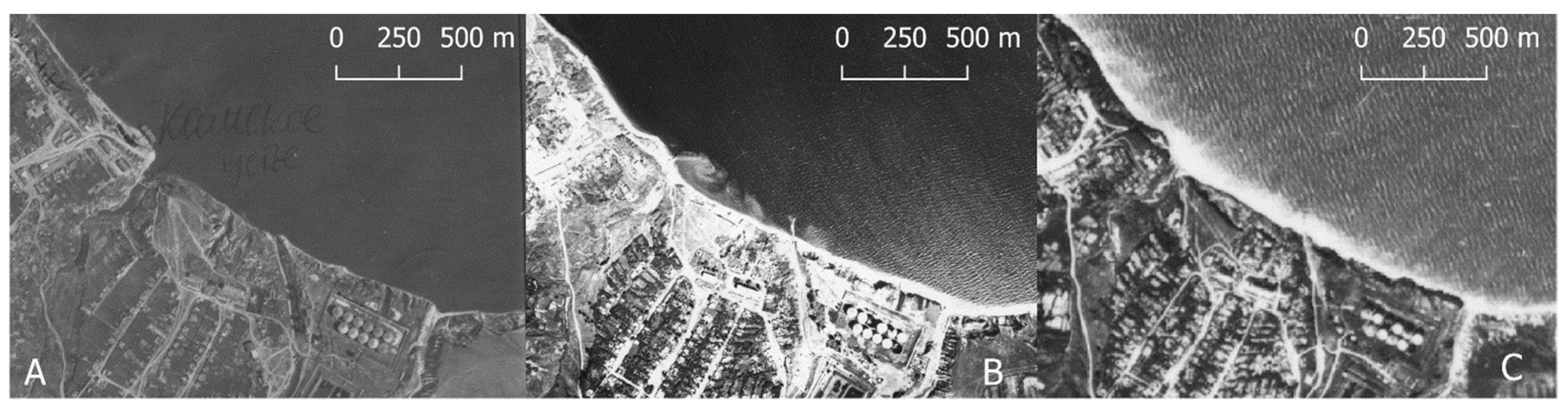
2. Study Area
3. Materials and Methods
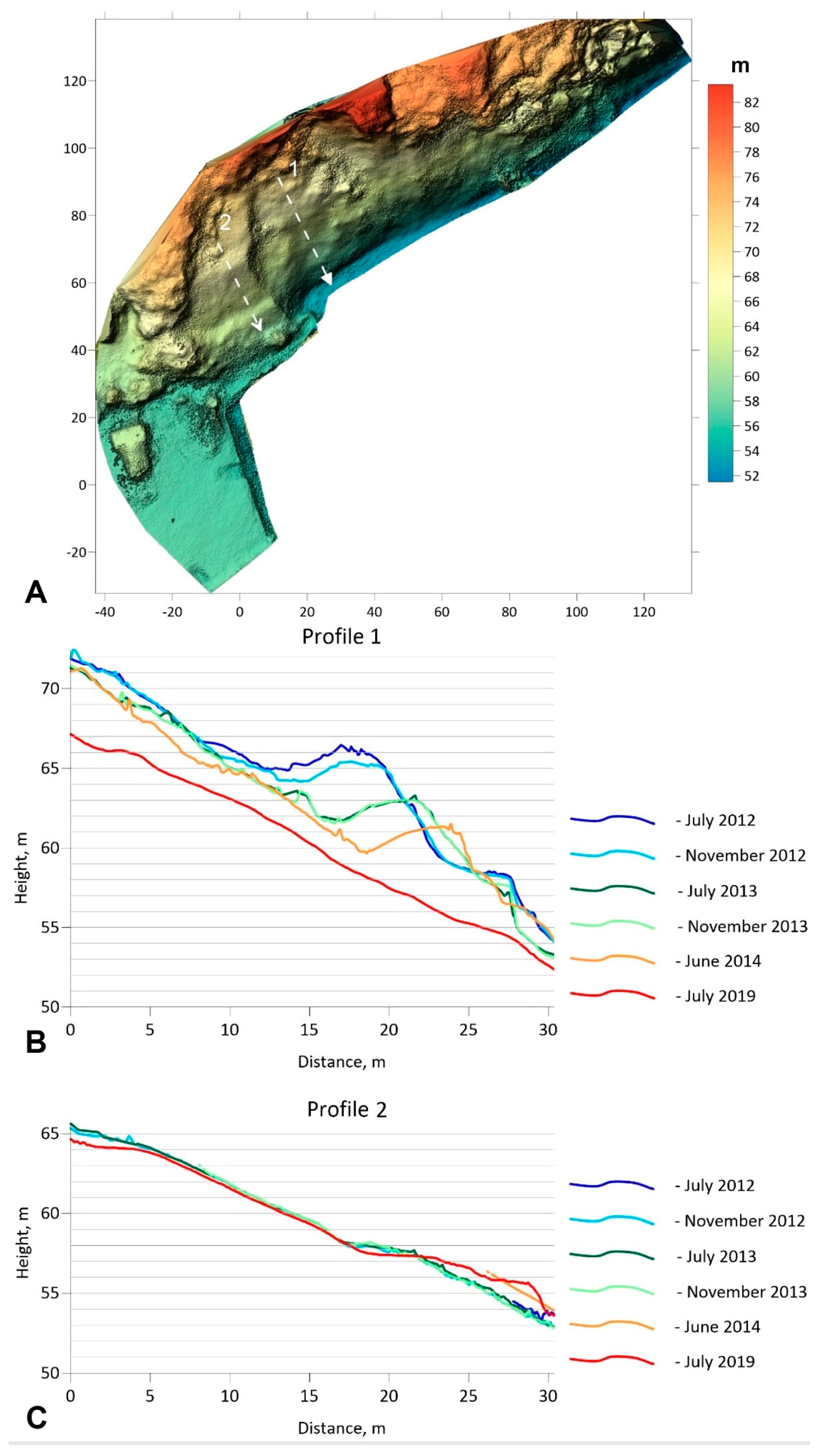
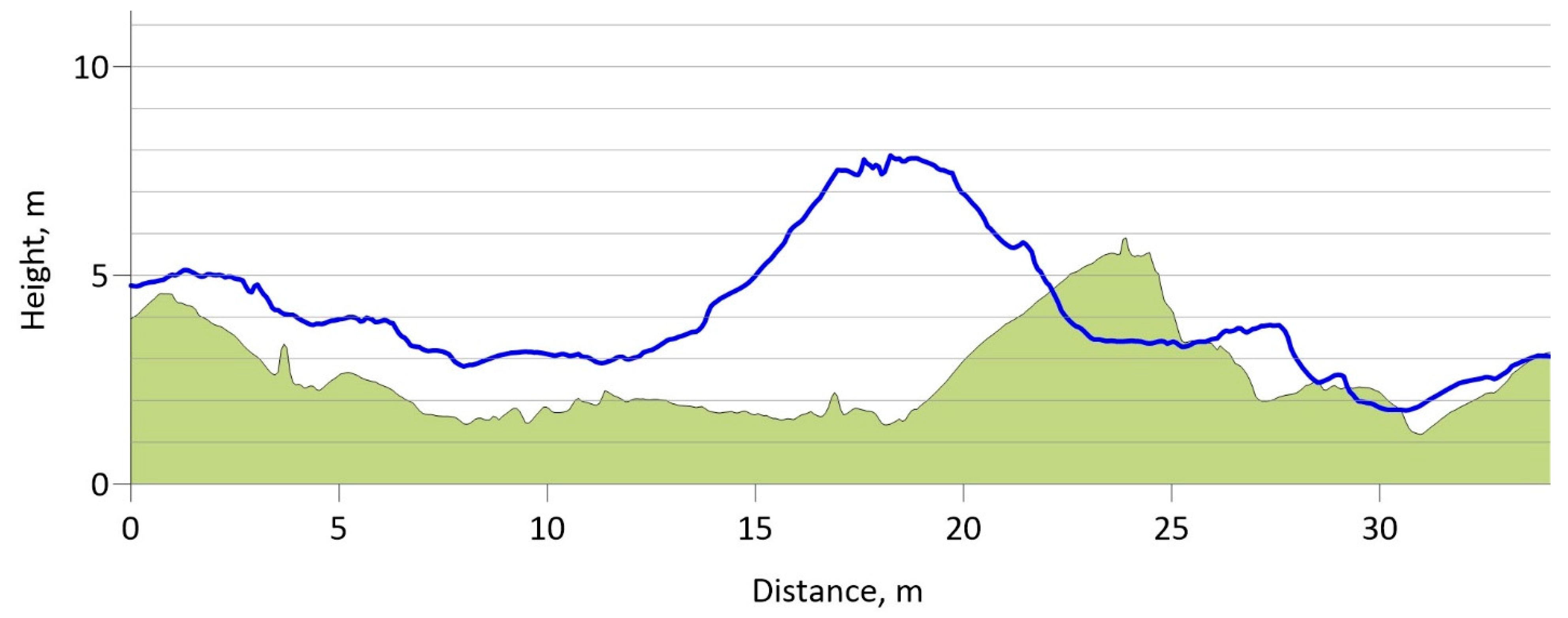
3.1. Site 1
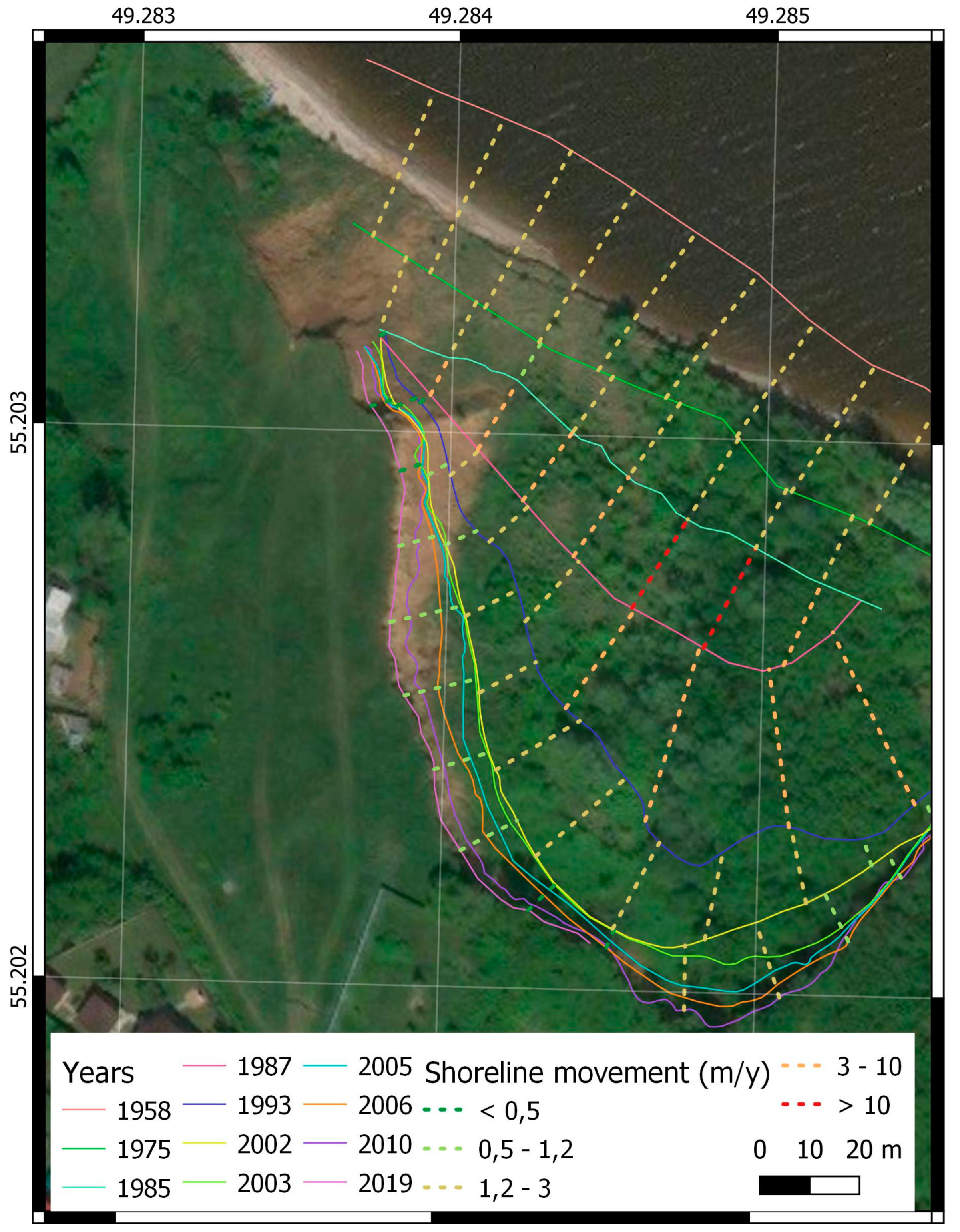
3.2. Site 2
4. Results
4.1. Observations at Site 1
4.2. Observations at Site 2
5. Discussion
6. Conclusions
Author Contributions
Funding
Data Availability Statement
Conflicts of Interest
References
- Yermolaev, O.; Usmanov, B. The basin approach to the anthropogenic impact assessment in oil-producing region. In Proceedings of the International Multidisciplinary Scientific GeoConference Surveying Geology and Mining Ecology Management, SGEM, Albena, Bulgaria, 17–26 June 2014; Volume 2, pp. 681–688. [Google Scholar]
- Yermolaev, O.; Usmanov, B.; Muharamova, S.S. The basin approach and mapping to the anthropogenic impact assessment on the east of the russian plain. Int. J. Appl. Eng. Res. 2015, 10, 41178–41184. [Google Scholar]
- Nicu, I.; Usmanov, B.; Gainullin, I.; Galimova, M. Shoreline dynamics and evaluation of cultural heritage sites on the shores of large reservoirs: Kuibyshev reservoir, russian federation. Water 2019, 11, 591. [Google Scholar] [CrossRef]
- Yermolaev, O.; Mukharamova, S.; Vedeneeva, E. River runoff modeling in the european territory of Russia. Catena 2021, 203, 105327. [Google Scholar] [CrossRef]
- Usmanov, B.; Nicu, I.C.; Gainullin, I.; Khomyakov, P. Monitoring and assessing the destruction of archaeological sites from kuibyshev reservoir coastline, Tatarstan Republic, Russian Federation. A Case Study. J. Coast. Conserv. 2018, 22, 417–429. [Google Scholar] [CrossRef]
- Gafurov, A.M.; Yermolayev, O.P. Automatic gully detection: Neural networks and computer vision. Remote Sens. 2020, 12, 1743. [Google Scholar] [CrossRef]
- Degraff, J.; Olson, E. Landslide monitoring techniques for wildland management. J. Soil Water Conserv. 1980, 35, 241–242. [Google Scholar]
- Scaioni, M. Modern Technologies for Landslide Monitoring and Prediction; Springer: Berlin/Heidelberg, Germany, 2015; ISBN 978-3-662-45930-0. [Google Scholar]
- Savvaidis, P. Existing landslide monitoring systems and techniques. Stars Earth Cult. 2003, 242–258. [Google Scholar]
- Tsai, Z.-X.; You, G.J.-Y.; Lee, H.-Y.; Chiu, Y.-J. Use of a total station to monitor post-failure sediment yields in landslide sites of the Shihmen Reservoir Watershed, Taiwan. Geomorphology 2012, 139–140, 438–451. [Google Scholar] [CrossRef]
- Pradhan, B. Laser Scanning Applications in Landslide Assessment; Springer International Publishing: Cham, Switzerland, 2017; ISBN 978-3-319-55341-2. [Google Scholar]
- Gafurov, A.M.; Rysin, I.I.; Golosov, V.N.; Grigoryev, I.I.; Sharifullin, A.G. Estimation of the recent rate of gully head retreat on the southern megaslope of the East European Plain using a set of instrumental methods. Vestn. Mosk. Univ. Seriya 5 Geogr. 2018, 61–71. [Google Scholar]
- Gupta, S.K.; Shukla, D.P. Application of drone for landslide mapping, dimension estimation and its 3D reconstruction. J. Indian Soc. Remote Sens. 2018, 46, 903–914. [Google Scholar] [CrossRef]
- Mertens, K.; Jacobs, L.; Maes, J.; Poesen, J.; Kervyn, M.; Vranken, L. Disaster risk reduction among households exposed to landslide hazard: A crucial role for self-efficacy? Land Use Policy 2018, 75, 77–91. [Google Scholar] [CrossRef]
- Casagli, N.; Frodella, W.; Morelli, S.; Tofani, V.; Ciampalini, A.; Intrieri, E.; Raspini, F.; Rossi, G.; Tanteri, L.; Lu, P. Spaceborne, UAV and ground-based remote sensing techniques for landslide mapping, monitoring and early warning. Geoenvironmental Disasters 2017, 4, 9. [Google Scholar] [CrossRef]
- Yang, I.T.; Park, J.K.; Kim, D.M. Monitoring the symptoms of landslide using the non-prism total station. KSCE J. Civ. Eng. 2007, 11, 293–301. [Google Scholar] [CrossRef]
- Bertacchini, E.; Capitani, A.; Capra, A.; Corsini, A.; Dubbini, M. Integrated surveying system for landslide monitoring, Valoria Landslide (Appennines of Modena, Italy). In Proceedings of the FIG Working Week, FIG Federation Internationale des Geometres, Eilat, Israel, 3–8 May 2009; Volume TS3F-n. 3343, p. 11. [Google Scholar]
- Barbarella, M.; Fiani, M. Monitoring of large landslides by terrestrial laser scanning techniques: Field data collection and processing. Eur. J. Remote Sens. 2013, 46, 126–151. [Google Scholar] [CrossRef]
- Chigira, M.; Duan, F.; Yagi, H.; Furuya, T. Using an Airborne laser scanner for the identification of shallow landslides and susceptibility assessment in an area of ignimbrite overlain by permeable pyroclastics. Landslides 2004, 1, 203–209. [Google Scholar] [CrossRef]
- Monserrat, O.; Crosetto, M. Deformation measurement using terrestrial laser scanning data and least squares 3d surface matching. ISPRS J. Photogramm. Remote Sens. 2008, 63, 142–154. [Google Scholar] [CrossRef]
- Dunning, S.A.; Massey, C.I.; Rosser, N.J. Structural and geomorphological features of landslides in the bhutan himalaya derived from terrestrial laser scanning. Geomorphology 2009, 103, 17–29. [Google Scholar] [CrossRef]
- Viero, A.; Teza, G.; Massironi, M.; Jaboyedoff, M.; Galgaro, A. Laser scanning-based recognition of rotational movements on a deep seated gravitational instability: The Cinque Torri case (North-Eastern Italian Alps). Geomorphology 2010, 122, 191–204. [Google Scholar] [CrossRef]
- Vaaja, M.; Hyyppä, J.; Kukko, A.; Kaartinen, H.; Hyyppä, H.; Alho, P. Mapping topography changes and elevation accuracies using a mobile laser scanner. Remote Sens. 2011, 3, 587–600. [Google Scholar] [CrossRef]
- Altuntas, C.; Karabork, H.; Tusat, E. Georeferencing of ground-based LIDAR data using continuously operating reference stations. Opt. Eng. 2014, 53, 1–8. [Google Scholar] [CrossRef][Green Version]
- Oppikofer, T.; Jaboyedoff, M.; Blikra, L.; Derron, M.-H.; Metzger, R. Characterization and monitoring of the Aknes rockslide using terrestrial laser scanning. Nat. Hazards Earth Syst. Sci. 2009, 9, 1003–1019. [Google Scholar] [CrossRef]
- Usmanov, B.; Yermolaev, O.; Gafurov, A. Estimates of slope erosion intensity utilizing terrestrial laser scanning. Proc. Int. Assoc. Hydrol. Sci. 2015, 367, 59–65. [Google Scholar] [CrossRef]
- Barbarella, M.; Fiani, M.; Lugli, A. Landslide monitoring using multitemporal terrestrial laser scanning for ground displacement analysis. Geomat. Nat. Hazards Risk 2015, 6, 398–418. [Google Scholar] [CrossRef]
- Gafurov, A.M.; Yermolaev, O.P.; Usmanov, B.M. Assessment of the intensity of slope erosion using terrestrial laser scanning. Int. J. Pharm. Technol. 2016, 8, 14822–14832. [Google Scholar]
- Gruen, A.; Akca, D. Least squares 3D surface and curve matching. ISPRS J. Photogramm. Remote Sens. 2005, 59, 151–174. [Google Scholar] [CrossRef]
- Pesci, A.; Teza, G.; Casula, G.; Loddo, F.; De Martino, P.; Dolce, M.; Obrizzo, F.; Pingue, F. Multitemporal laser scanner-based observation of the Mt. vesuvius crater: Characterization of overall geometry and recognition of landslide events. ISPRS J. Photogramm. Remote Sens. 2011, 66, 327–336. [Google Scholar] [CrossRef]
- Kociuba, W.; Kubisz, W.; Zagórski, P. Use of terrestrial laser scanning (TLS) for monitoring and modelling of geomorphic processes and phenomena at a small and medium spatial scale in polar environment (Scott River—Spitsbergen). Geomorphology 2014, 212, 84–96. [Google Scholar] [CrossRef]
- Michoud, C.; Carrea, D.; Costa, S.; Derron, M.-H.; Jaboyedoff, M.; Delacourt, C.; Maquaire, O.; Letortu, P.; Davidson, R. Landslide Detection and monitoring capability of boat-based mobile laser scanning along Dieppe Coastal Cliffs, Normandy. Landslides 2015, 12, 403–418. [Google Scholar] [CrossRef]
- Palenzuela, J.A.; Jiménez-Perálvarez, J.D.; El Hamdouni, R.; Alameda-Hernández, P.; Chacón, J.; Irigaray, C. Integration of LiDAR data for the assessment of activity in diachronic landslides: A case study in the Betic Cordillera (Spain). Landslides 2016, 13, 629–642. [Google Scholar] [CrossRef]
- Franz, M.; Carrea, D.; Abellán, A.; Derron, M.-H.; Jaboyedoff, M. Use of targets to track 3D displacements in highly vegetated areas affected by landslides. Landslides 2016, 13, 821–831. [Google Scholar] [CrossRef]
- Yermolaev, O.P.; Gafurov, A.M.; Usmanov, B.M. Evaluation of erosion intensity and dynamics using terrestrial laser scanning. Eurasian Soil Sci. 2018, 51, 814–826. [Google Scholar] [CrossRef]
- Spreafico, M.C.; Perotti, L.; Cervi, F.; Bacenetti, M.; Bitelli, G.; Girelli, V.A.; Mandanici, E.; Tini, M.A.; Borgatti, L. Terrestrial remote sensing techniques to complement conventional geomechanical surveys for the assessment of landslide hazard: The San Leo case study (Italy). Eur. J. Remote Sens. 2015, 48, 639–660. [Google Scholar] [CrossRef]
- Wang, X.; Pedrycz, W.; Niu, R. Spatio-temporal analysis of quaternary deposit landslides in the Three Gorges. Nat. Hazards 2015, 75, 2793–2813. [Google Scholar] [CrossRef]
- Zhang, Y.; Zhu, S.; Tan, J.; Li, L.; Yin, X. The influence of water level fluctuation on the stability of landslide in the Three Gorges reservoir. Arab. J. Geosci. 2020, 13, 845. [Google Scholar] [CrossRef]
- Guo, Z.; Chen, L.; Yin, K.; Shrestha, D.P.; Zhang, L. Quantitative risk assessment of slow-moving landslides from the viewpoint of decision-making: A case study of the Three Gorges reservoir in China. Eng. Geol. 2020, 273, 105667. [Google Scholar] [CrossRef]
- Starodubtsev, V.M. Impact of Bugun’ water reservoir on coast for 50 years. Arid Ecosyst. 2012, 2, 132–138. [Google Scholar] [CrossRef]
- Babicheva, V.A.; Rzetala, M.A. The main types of banks of Angara water reservoirs: Overview of the problem. Int. Multidiscip. Sci. GeoConference SGEM 2013, 1, 195–202. [Google Scholar] [CrossRef]
- Kalinin, V.G.; Nazarov, N.N.; Pyankov, S.V.; Simirenov, S.A.; Tynyatkin, D.G. activity of the landslide on the bank of the Kamskoe Storage reservoir according to stationary measurements and GIS-technology application. Geomorphol. RAS 2015, 55–62. [Google Scholar] [CrossRef]
- Bondur, V.G.; Zakharova, L.N.; Zakharov, A.I.; Chimitdorzhiev, T.N.; Dmitriev, A.V.; Dagurov, P.N. Monitoring of landslide processes by means of L-band radar interferometric observations: Bureya River bank caving case. Issled. Zemli Iz Kosmosa 2019, 3–14. [Google Scholar] [CrossRef]
- Mazaeva, O.; Babicheva, V.; Kozyreva, E. Geomorphological process development under the impact of man-made reservoir operation, a case study: Bratsk Reservoir, Baikal-Angara hydroengineering system, Russia. Bull. Eng. Geol. Environ. 2019, 78, 4659–4672. [Google Scholar] [CrossRef]
- Nikonorova, I.V.; Petrov, N.F.; Gumenyuk, A.E.; Ilyin, V.N. Sustainable use of natural resources in a hazardous landslide slopes of Cheboksary reservoir (River Volga). In Proceedings of the International Conference on Extraction, Transport, Storage and Processing of Hydrocarbons and Minerals, Tyumen, Russia, 19–20 August 2019; Volume 663, p. 012043. [Google Scholar] [CrossRef]
- Marzolff, I.; Poesen, J. The potential of 3D gully monitoring with GIS using high-resolution aerial photography and a digital photogrammetry system. Geomorphology 2009, 111, 48–60. [Google Scholar] [CrossRef]
- Marzolff, I.; Ries, J.B.; Poesen, J. Short-term versus medium-term monitoring for detecting gully-erosion variability in a mediterranean environment. Earth Surf. Process. Landf. 2011, 36, 1604–1623. [Google Scholar] [CrossRef]
- Gafurov, A.M. Possible use of unmanned aerial vehicle for soil erosion assessment. Uchenye Zap. Kazan. Univ.-Seriya Estestv. Nauki 2017, 159, 654–667. [Google Scholar]
- Eker, R.; Aydın, A.; Hübl, J. Unmanned aerial vehicle (UAV)-based monitoring of a landslide: Gallenzerkogel landslide (Ybbs-Lower Austria) case study. Environ. Monit. Assess. 2018, 190, 28. [Google Scholar] [CrossRef]
- Agisoft PhotoScan User Manual—Professional Edition, version 1.4; Agisoft LLC: St. Petersburg, Russia, 2018.
- Bradski, G.; Kaehler, A. Learning OpenCV: Computer Vision with the OpenCV Library, Software that Sees, 1st ed.; O’Reilly: Sebastopol, CA, USA, 2011; ISBN 978-0-596-51613-0. [Google Scholar]
- D’Oleire-Oltmanns, S.; Marzolff, I.; Peter, K.D.; Ries, J.B.; Hssaïne, A.A. Monitoring soil erosion in the Souss Basin, Morocco, with a multiscale object-based remote sensing approach using UAV and satellite data. In Proceedings of the 1st World Sustainability Forum, Basel, Switzerland, 1–15 November 2011; pp. 1–13. [Google Scholar]
- D’Oleire-Oltmanns, S.; Marzolff, I.; Peter, K.; Ries, J. Unmanned aerial vehicle (UAV) for monitoring soil erosion in Morocco. Remote Sens. 2012, 4, 3390–3416. [Google Scholar] [CrossRef]
- Fritz, A.; Kattenborn, T.; Koch, B. UAV-based photogrammetric point clouds—Tree stem mapping in open stands in comparison to terrestrial laser scanner point clouds. In Proceedings of the International Archives of the Photogrammetry, Remote Sensing and Spatial Information Sciences, Rostock, Germany, 4–6 September 2013; Volume V XL-1/W2, pp. 141–146. [Google Scholar] [CrossRef]
- Vasuki, Y.; Holden, E.-J.; Kovesi, P.; Micklethwaite, S. Semi-automatic mapping of geological structures using UAV-based photogrammetric data: An image analysis approach. Comput. Geosci. 2014, 69, 22–32. [Google Scholar] [CrossRef]
- Savin, I.; Prudnikova, E.; Chendev, Y.; Bek, A.; Kucher, D.; Dokukin, P. Detection of changes in arable chernozemic soil health based on landsat TM archive data. Remote Sens. 2021, 13, 2411. [Google Scholar] [CrossRef]
- Terekhin, E.A. Spectral response of abandoned arable lands in various climate and environmental conditions of European Russia. Sovrem. Probl. Distantsionnogo Zondirovaniya Zemli Kosmosa 2021, 18, 169–181. [Google Scholar] [CrossRef]
- Gruszczyński, W.; Matwij, W.; Ćwiąkała, P. Comparison of low-altitude uav photogrammetry with terrestrial laser scanning as data-source methods for terrain covered in low vegetation. ISPRS J. Photogramm. Remote Sens. 2017, 126, 168–179. [Google Scholar] [CrossRef]
- Gafurov, A.M. Small catchments DEM creation using unmanned aerial vehicles. In Proceedings of the 3rd International Conference Environment and Sustainable Development of Territories: Ecological Challenges of the 21st Century, Kazan, Russia, 27–29 September 2017; Volume 107, p. 012005. [Google Scholar] [CrossRef]
- Lucieer, A.; Turner, D.; King, D.H.; Robinson, S.A. Using an unmanned aerial vehicle (UAV) to capture micro-topography of Antarctic Moss Beds. Int. J. Appl. Earth Obs. Geoinformation 2014, 27, 53–62. [Google Scholar] [CrossRef]
- Richter, N.; Favalli, M.; de Zeeuw-van Dalfsen, E.; Fornaciai, A.; da Silva Fernandes, R.M.; Pérez, N.M.; Levy, J.; Victória, S.S.; Walter, T.R. Lava flow hazard at Fogo Volcano, Cabo Verde, before and after the 2014–2015 eruption. Nat. Hazards Earth Syst. Sci. 2016, 16, 1925–1951. [Google Scholar] [CrossRef]
- Müller, D.; Walter, T.R.; Schöpa, A.; Witt, T.; Steinke, B.; Gudmundsson, M.T.; Dürig, T. High-resolution digital elevation modeling from TLS and UAV campaign reveals structural complexity at the 2014/2015 Holuhraun Eruption Site, Iceland. Front. Earth Sci. 2017, 5, 59. [Google Scholar] [CrossRef]
- Cawood, A.J.; Bond, C.E.; Howell, J.A.; Butler, R.W.H.; Totake, Y. LiDAR, UAV or Compass-clinometer? Accuracy, coverage and the effects on structural models. J. Struct. Geol. 2017, 98, 67–82. [Google Scholar] [CrossRef]
- James, M.R.; Robson, S. Mitigating systematic error in topographic models derived from UAV and ground-based image networks. Earth Surf. Process. Landf. 2014, 39, 1413–1420. [Google Scholar] [CrossRef]
- Udin, W.S.; Ahmad, A. Assessment of photogrammetric mapping accuracy based on variation flying altitude using unmanned aerial vehicle. In Proceedings of the 8th International Symposium of the Digital Earth, Kuching, Malaysia, 26–29 August 2014; Volume 18, pp. 1–7. [Google Scholar] [CrossRef]
- Uysal, M.; Toprak, A.S.; Polat, N. DEM generation with UAV photogrammetry and accuracy analysis in Sahitler Hill. Measurement 2015, 73, 539–543. [Google Scholar] [CrossRef]
- Gindraux, S.; Boesch, R.; Farinotti, D. Accuracy assessment of digital surface models from unmanned aerial vehicles’ imagery on glaciers. Remote Sens. 2017, 9, 186. [Google Scholar] [CrossRef]
- Benassi, F.; Dall’Asta, E.; Diotri, F.; Forlani, G.; Morra di Cella, U.; Roncella, R.; Santise, M. Testing accuracy and repeatability of UAV blocks oriented with GNSS-supported aerial triangulation. Remote Sens. 2017, 9, 172. [Google Scholar] [CrossRef]
- Turner, D.; Lucieer, A.; Watson, C. An automated technique for generating georectified mosaics from ultra-high resolution unmanned aerial vehicle (UAV) imagery, based on structure from motion (SfM) point clouds. Remote Sens. 2012, 4, 1392–1410. [Google Scholar] [CrossRef]
- Gafurov, A. The methodological aspects of constructing a high-resolution DEM of large territories using low-cost UAVs on the example of the sarycum aeolian complex, Dagestan, Russia. Drones 2021, 5, 7. [Google Scholar] [CrossRef]
- Agüera-Vega, F.; Carvajal-Ramírez, F.; Martínez-Carricondo, P.; Sánchez-Hermosilla López, J.; Javier Mesas-Carrascosa, F.; García-Ferrer, A.; Juan Pérez-Porras, F. Reconstruction of extreme topography from UAV structure from motion photogrammetry. Measurement 2018, 121, 127–138. [Google Scholar] [CrossRef]
- Yermolaev, O.P. Geoinformation Mapping of soil erosion in the Middle Volga region. Eurasian Soil Sci. 2017, 50, 118–131. [Google Scholar] [CrossRef]
- Cruden, D.; Varnes, D. Landslide Types and Processes; Special Report; National Academy Press: Washington, DC, USA, 1996; Dalam: Turner, AK Landslides Investigation and Mitigation. [Google Scholar]
- Peppa, M.V.; Mills, J.P.; Moore, P.; Miller, P.E.; Chambers, J.E. Accuracy assessment of a UAV-based landslide monitoring system. ISPRS—Int. Arch. Photogramm. Remote Sens. Spat. Inf. Sci. 2016, XLI-B5, 895–902. [Google Scholar] [CrossRef]
- Zang, Y.; Yang, B.; Li, J.; Guan, H. An accurate TLS and UAV image point clouds registration method for deformation detection of chaotic hillside areas. Remote Sens. 2019, 11, 647. [Google Scholar] [CrossRef]
- Himmelstoss, E.A.; Henderson, R.; Kratzmann, M.; Farris, A. Digital Shoreline Analysis System; Version 5; Reston, VA, USA, 2018. [Google Scholar]
- Oyedotun, T.D.T. Shoreline geometry: DSAS as a tool for historical trend analysis. Geomorphol. Tech. Online Ed. 2014, 3, 1–12. [Google Scholar]
- Nicu, I.C. Is digital shoreline analysis system “Fit” for gully erosion assessment? CATENA 2021, 203, 105307. [Google Scholar] [CrossRef]
- Ragozin, A.L.; Burova, V.N. A method for approximate forecast of reservoir bank destruction. J. Gidrotekhnicheskoe Stroit. 1993, 10, 20–26. [Google Scholar]
- Broeckx, J.; Maertens, M.; Isabirye, M.; Vanmaercke, M.; Namazzi, B.; Deckers, J.; Tamale, J.; Jacobs, L.; Thiery, W.; Kervyn, M.; et al. Landslide susceptibility and mobilization rates in the Mount Elgon Region, Uganda. Landslides 2019, 16, 571–584. [Google Scholar] [CrossRef]
- Broeckx, J.; Rossi, M.; Lijnen, K.; Campforts, B.; Poesen, J.; Vanmaercke, M. Landslide mobilization rates: A global analysis and model. Earth-Sci. Rev. 2020, 201, 102972. [Google Scholar] [CrossRef]
- Devoto, S.; Macovaz, V.; Mantovani, M.; Soldati, M.; Furlani, S. Advantages of using UAV digital photogrammetry in the study of slow-moving coastal landslides. Remote Sens. 2020, 12, 3566. [Google Scholar] [CrossRef]
- Gili, J.A.; Corominas, J.; Rius, J. Using global positioning system techniques in landslide monitoring. Eng. Geol. 2000, 55, 167–192. [Google Scholar] [CrossRef]
- Burova, V.N. Abrasion risk assessment on the coasts of seas and water reservoirs. Geod. List 2020, 74, 185–198. [Google Scholar]
- Ovchinnikov, G.I.; Maksimishina, Y.S. The importance of geological-geomorphological factors in the development of abrasion processes on the coasts of the Bratsk Reservoir, in the SE part of Russia. Landf. Anal. 2002, 3. [Google Scholar]
- Middle Volga. Geomorphological Guidebook; Dedkov, A.P., Ed.; in Russian; Publishing House of Kazan University: Kazan, Russia, 1991. [Google Scholar]
- Kotlyakov, A.V.; Shumakova, E.M.; Artem’ev, S.A. Dynamics of the coastal zone of the Kuibyshev and Saratov reservoirs in the Tolyatti Area and Its correlation with the operation regime of the Zhigulevskaya HPP. Water Resour. 2007, 34, 657–662. [Google Scholar] [CrossRef]
- Gaynullin, I.; Sitdikov, A.; Usmanov, B. Destructive abrasion processes study in archaeological sites placement (Kuibyshev and Nizhnekamsk Reservoirs, Russia). In Proceedings of the International Multidisciplinary Scientific Conference on Social Sciences & Arts SGEM, Albena, Bulgaria, 2–7 September 2014; pp. 339–346. [Google Scholar]
- Gaynullin, I.I.; Sitdikov, A.G.; Usmanov, B.M. Abrasion processes of Kuibyshev Reservoir as a factor of destruction of archaeological site Ostolopovo (Tatarstan, Russia). Adv. Environ. Biol. 2014, 8, 1027–1030. [Google Scholar]
- Bespalova, K.V.; Selezneva, A.V.; Seleznev, V.A. Influence of the water discharge of the Kuibyshev reservoir on the dynamics of the ecosystem of the Seredysh and Bakhilovsky Islands, the Volga River, Russia. In Proceedings of the 4th Conference on Actual problems of specially protected natural areas, Togljatti, Russia, 17–18 September 2020; Volume 607, p. 012017. [Google Scholar] [CrossRef]


| Scan Date | Site 1 (#) |
|---|---|
| July 2012 | 1,847,951 |
| November 2012 | 2,271,130 |
| July 2013 | 850,394 |
| November 2013 | 1,509,131 |
| June 2014 | 1,550,689 |
| Year—Month | Type of Measurement |
|---|---|
| 2012-July, November | Laser Scan |
| 2013-July, November | Laser Scan |
| 2014-June | Laser scanning |
| 2019-August | UAV |
| Point № | Manual Point Selection | Iterative Closest Point Method (ICP) | ||||
|---|---|---|---|---|---|---|
| X (m) | Y (m) | Z (m) | X (m) | Y (m) | Z (m) | |
| 1 | 0.09 | −0.18 | 0.63 | −0.05 | 0.11 | −0.20 |
| 2 | −0.45 | 0.09 | 0.18 | 0.10 | 0.00 | 0.01 |
| 3 | 0.09 | 0.27 | −0.36 | 0.00 | 0.16 | 0.12 |
| 4 | 0.27 | −0.36 | 0.45 | −0.04 | 0.10 | −0.19 |
| 5 | 0.36 | 0.45 | −0.54 | −0.11 | −0.28 | −0.16 |
| 6 | 0.54 | 0.27 | 0.09 | 0.06 | −0.13 | 0.07 |
| 7 | −0.18 | 0.09 | 0.09 | −0.03 | −0.06 | 0.03 |
| Total | 0.28 | 0.24 | 0.33 | 0.06 | 0.12 | 0.11 |
| Year | Source Data |
|---|---|
| 1958 | Aerial image |
| 1975 | “Corona” satellite image |
| 1985 | Aerial image |
| 1987 | Aerial image |
| 1993 | Aerial image |
| 2002 | Total Station Survey |
| 2003 | Total Station Survey |
| 2005 | Total Station Survey |
| 2006 | Total Station Survey |
| 2010 | Roscosmos satellite image |
| 2019 | UAV data |
| Observation Period | Abrasion Scarp | Upper Part of the Slope V− S−1, m3 m−2 | |
|---|---|---|---|
| V− S−1 *, m3 m−2 | V+ S−1 *, m3 m−2 | ||
| 06/2012–11/2012 | 0.08 | 0.25 | 0.06 |
| 11/2012–06/2013 | 0.67 | 0.06 | 0.2 |
| 06/2012–07/2013 ** | 0.54 | 0.05 | 0.25 |
| 07/2013–11/2013 | 0.02 | 0.02 | 0.08 |
| 11/2013–06/2014 | 0.03 | 0.69 | 0.08 |
| 07/2013–06/2014 | 0.07 | 0.61 | 0.17 |
| Observation Period | V+ S−1 *, m3 m−2 | V− S−1 *, m3 m−2 | ΔV S−1 m3 m−2 |
|---|---|---|---|
| 06/2012–11/2012 | 0.008 | 0.017 | −0.009 |
| 11/2012–7/2013 | 0.014 | 0.036 | −0.023 |
| 06/2012–07/2013 ** | 0.012 | 0.044 | −0.033 |
| 7/2013–11/2013 | 0.003 | 0.022 | −0.019 |
| 11/2013–6/2014 | 0.014 | 0.026 | −0.012 |
| 07/2013–06/2014 | 0.009 | 0.040 | −0.031 |
| 6/2014–8/2019 | 0.000 | 0.038 | −0.038 |
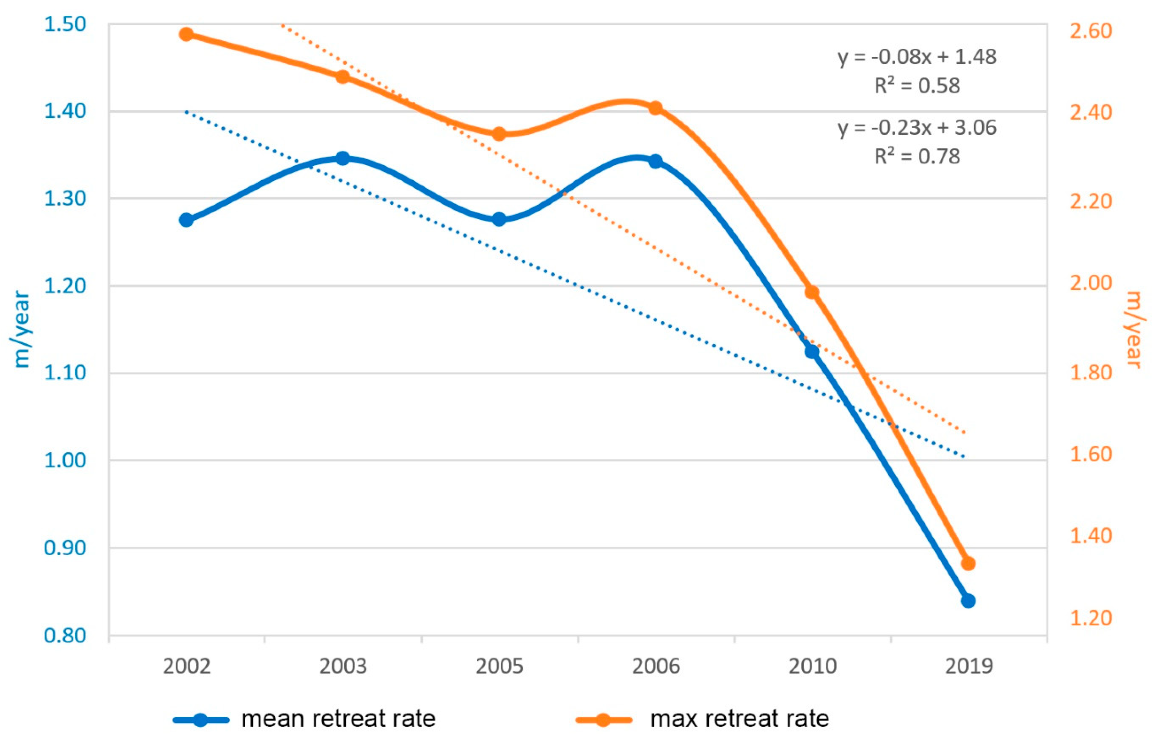
| Year | Retreat Rate (m yr−1) | |
|---|---|---|
| Mean | Maximum | |
| 1975 | 1.89 | 2.12 |
| 1985 | 1.45 | 1.92 |
| 1987 | 8.73 | 11.29 |
| 1993 | 3.50 | 6.38 |
| 2002 | 1.28 | 2.67 |
| 2003 | 1.35 | 2.57 |
| 2005 | 1.28 | 2.43 |
| 2006 | 1.34 | 2.49 |
| 2010 | 1.12 | 2.04 |
| 2019 | 0.84 | 1.38 |
Publisher’s Note: MDPI stays neutral with regard to jurisdictional claims in published maps and institutional affiliations. |
© 2021 by the authors. Licensee MDPI, Basel, Switzerland. This article is an open access article distributed under the terms and conditions of the Creative Commons Attribution (CC BY) license (https://creativecommons.org/licenses/by/4.0/).
Share and Cite
Yermolaev, O.; Usmanov, B.; Gafurov, A.; Poesen, J.; Vedeneeva, E.; Lisetskii, F.; Nicu, I.C. Assessment of Shoreline Transformation Rates and Landslide Monitoring on the Bank of Kuibyshev Reservoir (Russia) Using Multi-Source Data. Remote Sens. 2021, 13, 4214. https://doi.org/10.3390/rs13214214
Yermolaev O, Usmanov B, Gafurov A, Poesen J, Vedeneeva E, Lisetskii F, Nicu IC. Assessment of Shoreline Transformation Rates and Landslide Monitoring on the Bank of Kuibyshev Reservoir (Russia) Using Multi-Source Data. Remote Sensing. 2021; 13(21):4214. https://doi.org/10.3390/rs13214214
Chicago/Turabian StyleYermolaev, Oleg, Bulat Usmanov, Artur Gafurov, Jean Poesen, Evgeniya Vedeneeva, Fedor Lisetskii, and Ionut Cristi Nicu. 2021. "Assessment of Shoreline Transformation Rates and Landslide Monitoring on the Bank of Kuibyshev Reservoir (Russia) Using Multi-Source Data" Remote Sensing 13, no. 21: 4214. https://doi.org/10.3390/rs13214214
APA StyleYermolaev, O., Usmanov, B., Gafurov, A., Poesen, J., Vedeneeva, E., Lisetskii, F., & Nicu, I. C. (2021). Assessment of Shoreline Transformation Rates and Landslide Monitoring on the Bank of Kuibyshev Reservoir (Russia) Using Multi-Source Data. Remote Sensing, 13(21), 4214. https://doi.org/10.3390/rs13214214