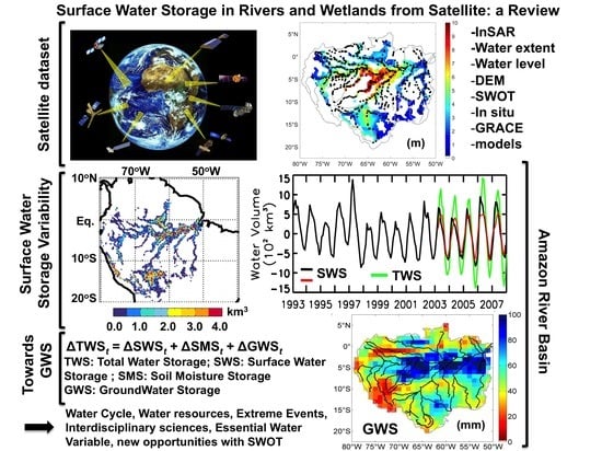
Surface Water Storage in Rivers and Wetlands Derived from Satellite Observations: A Review of Current Advances and Future Opportunities for Hydrological Sciences

Abstract

Surface water storage (SWS), the amount of freshwater stored in rivers/wetlands/floodplains/lakes, and its variations are key components of the water cycle and land surface hydrology, with strong feedback and linkages with climate variability. They are also very important for water resources management. However, it is still very challenging to measure and to obtain accurate estimates of SWS variations for large river basins at adequate time/space sampling. Satellite observations offer great opportunities to measure SWS changes, and several methods have been developed combining multisource observations for different environments worldwide. With the upcoming launch in 2022 of the Surface Water and Ocean Topography (SWOT) satellite mission, which will provide, for the first time, direct estimates of SWS variations with an unprecedented spatial resolution (~100 m), it is timely to summarize the recent advances in the estimates of SWS from satellite observations and how they contribute to a better understanding of large-scale hydrological processes. Here, we review the scientific literature and present major results regarding the dynamic of surface freshwater in large rivers, floodplains, and wetlands. We show how recent efforts have helped to characterize the variations in SWS change across large river basins, including during extreme climatic events, leading to an overall better understanding of the continental water cycle. In the context of SWOT and forthcoming SWS estimates at the global scale, we further discuss new opportunities for hydrological and multidisciplinary sciences. We recommend that, in the near future, SWS should be considered as an essential water variable to ensure its long-term monitoring.

1. Introduction

Freshwater is crucial to terrestrial life, ecosystem environments, biodiversity, and human societies [1,2,3,4,5]. Freshwater on land is stored in various reservoirs, unevenly distributed across climates and geophysical environments [6,7,8]. About 70% of global freshwater is stored in reservoirs with relatively long retention periods, namely, ice caps, glaciers, permanent snow, aquifers, and other geological formations [9,10]. Freshwater stored with much shorter retention times is found in seasonal snow, soil moisture of the root zone (the upper few meters of the soil where the plants absorb water and nutrients or the unsaturated zone), shallow groundwater, and surface waters. The latter includes rivers, lakes, wetlands, floodplains and inundated areas, and manmade reservoirs [11]. All these components are continuously exchanging mass by vertical and horizontal motions with the atmosphere and the oceans, making them an integral part of the global water cycle [12,13,14]. They are also key players in the climate system with major links and feedback with climate variability [6,8] and water resources [15].

Freshwater availability is generally highly seasonal, strongly driven by local or remote rainfall, and it is subject to strong variability across time scales [16], from daily to interannual and decadal changes [17], often modulated by alternate periods of floods or droughts [18,19]. In the last few decades, the impacts of climate change and anthropogenic pressure, such as the increasing demand for freshwater supply worldwide, have made freshwater availability a current major global concern [17,20,21,22,23,24,25,26]. In several regions, water management is problematic due to the growing demands for a continually increasing population and needs for the agriculture, energy, and industrial sectors [27,28,29], with major consequences for water quality [30].

Therefore, understanding the flow, spatial distribution, and storage of freshwater on land is key for characterizing the terrestrial branch of the global water cycle [11,31,32], as well as for an effective management of water resources [33], and an improved description of the components of the continental water cycle is now recognized as being of major importance. However, the distribution and spatiotemporal variations in terrestrial water storage are still poorly known at a regional to global scale, leaving open several fundamental questions regarding the land water storage budget: How much freshwater is stored at the surface and subsurface of continents? What are the spatial and temporal dynamics of terrestrial water storage? How do they interact with climate variability and anthropogenic pressure?

The terrestrial water balance equation [34], as applied to a river basin, can be written as

P − E = Q + ΔTWS,

(1)

where P and E represent the basin-averaged precipitation and evapotranspiration, respectively, Q is the discharge across the basin boundary (including river and groundwater discharge), and TWS is the total water storage, encompassing total surface and subsurface storages (sum of soil moisture, snow water content, surface water storage, vegetation water content, groundwater, and glaciers [35]). In most cases, each quantity is available only with a large uncertainty [32,36,37], and the estimation of the storage change term is particularly problematic, limiting our ability to understand its impacts on evapotranspiration, infiltration, and runoff. Quantifying water storage globally over long time periods, with consideration of surface and subsurface water volume dynamics, is fundamental [32]. For instance, surface water remains the main contributor to storage variability in large-scale water budgets at seasonal and interannual scales [38,39].

Historically, our knowledge of the spatiotemporal variations of continental water height, extent, and storage relies on in situ observations. In situ gauge measurements indeed help quantify the movement of water discharge in river channels but provide comparatively little information about the spatial dynamics of terrestrial water in floodplains and wetlands or groundwater, largely because of the prohibitive cost and complexity of monitoring large systems such as floodplains and aquifers. In addition, in situ networks are sparse, and the availability of ground-based gauge information has dramatically decreased during the last decades [31], particularly in remote areas with difficult access. In some cases, public access to data for several important rivers is restricted and not available to the scientific community, often due to political situations or transboundary water sharing conditions [40]. Until recently, lacking spatial measurements of inundation/wetland locations, sizes, and water volume changes limited the development of hydrologic models, which are often unable to properly partition precipitation (minus evapotranspiration) among the several freshwater components and represent their effects on river discharge at continental to global scales [31,41,42,43]. Despite several recent advances [44,45], our ability to measure, to monitor, and to forecast supplies of freshwater using hydrological models is still facing difficulties, at least at large scales [46,47].

In this context, spatial remote sensing techniques are a cost-effective method for monitoring the terrestrial water cycle, with high temporal coverage and reasonable accuracy. The large-scale coverage of areas by the satellite data helps in particular to understand the spatiotemporal variations of freshwater stored on land [48,49]. Since 2002, the Gravity Recovery and Climate Experiment (GRACE) provides, for the first time, precise measurements of the spatiotemporal variations in total terrestrial water storage (TWS) at basin scales [50]. Long-term time series enable us to study changes at the global scale and depict emerging trends in TWS changes linked to environmental or human disturbances [17,51,52,53]. TWS change results from the contribution of changes in the other water storage compartments [54], including groundwater storage (GWS), soil moisture storage (SMS), surface water storage (SWS), and ice and snow storage (ISS) changes, such that over a period of time (t), the change in TWS can be decomposed as

ΔTWS_t = ΔSWS_t + ΔSMS_t + ΔISS_t + ΔGWS_t.

(2)

Individually, the variations and changes in each of these reservoirs can also be estimated from remote sensing observations. For instance, snow water equivalent, the volume of water contained in the snowpack, has long been monitored in snow-covered regions throughout the world [55], especially in vast boreal regions [56], providing time series since 1978 following the launch of passive microwave sensors such as the Scanning Multichannel Microwave Radiometer (SMMR), Special Sensor Microwave/Imager (SSM/I), and Special Sensor Microwave Imager/Sounder (SSMIS) instruments. Soil moisture storage has also long been monitored and has even benefited from the launch of dedicated satellite missions, such as the Soil Moisture and Ocean Salinity (SMOS) [57] or Soil Moisture Active Passive (SMAP) [58] missions. Despite some limitations, these quantities and their variations are nevertheless fairly known, to some extent, from local to global scale.

Surprisingly, SWS, despite its importance, still suffers from a limited knowledge of its variations and changes, and the spatiotemporal variations of the surface freshwater reservoir are still widely unknown, at least from regional to global scale [59,60]. This is even more striking since, already more than a decade ago, Ref. [11] pointed out that, “given societies’ basic need for freshwater, perhaps the most important hydrologic observations that can be made are of the temporal and spatial variations in water stored in rivers, lakes, reservoirs, floodplains, and wetlands”. The lack of information regarding the amount of water stored and moving through the surface water bodies of large river basins prevents progress to understand the role of wetlands in the carbon balance, and how surface water affects biogeochemical and trace gas fluxes between the land and atmosphere and transport to the oceans [61,62]. The amount of water transported through large floodplains and wetlands is also key to understand the dissolved and particulate material (sediment and organic matter) exchanges with the main river channel [63,64], as well as the effect they have on the local climate by modulating atmospheric temperatures and contributing to increased evaporation [65,66]. They also impact basin hydrology due to storage effects along channel reaches, by regulating the size and timing of the annual flood wave, thus serving as a driver of ecology and biotic communities [67,68]. Human activities can alter the ecological services of floodplains by modifying channel and floodplain connectivity and reducing the role of storage in modulating fluxes of waters, sediment, and nutrients, with strong impacts on the environment [69].

Additionally, as mentioned above, accurate partitioning of GRACE-derived TWS into the different water storage contributions is needed, especially to quantify GWS variations [70]. Several approaches using auxiliary information on the other components of TWS, from either in situ observations or land-surface models, have been used to produce a time series of groundwater storage anomalies [51,71,72], especially in regions where human pressure on GWS is important, such as northern India [73,74] or in Bangladesh [75]. However, as the contribution of SWS to TWS can be substantial, sometimes up to 50%, especially in humid environments and in monsoon-dominated river basins [39,76,77,78], the lack of quantification of SWS changes prevents accurate GWS estimates from GRACE data.

Surface hydrology studies traditionally use remote sensing to map the extent and elevation of water bodies and their changes over time [11,30]. Since the late 1990s, radar altimetry missions provide monitoring of water levels of lakes, large rivers, and floodplains [79]. Today, radar altimetry potentially provides long-term monitoring of surface water elevation over almost three decades at thousands of Virtual Stations (VS). Additionally, lidar and interferometric synthetic aperture radar (InSAR) have been deployed on airborne and satellite platforms to measure elevations of water bodies [80]. In parallel, many developments, using satellite observations, made in a wide range of the electromagnetic spectrum (visible, infrared, and microwave), have been carried to monitor the extent and dynamics of surface water bodies, with varying degrees of success [30,81,82,83]. Multi-satellite remote sensing techniques also provide important information on the spatial and temporal variations of land surface waters at the global scale [84,85,86].

Combining such satellite-derived observations on surface water extent and elevation, efforts have been undertaken to quantify the variations of SWS, from seasonal to interannual time scales, for some large river basins. Curiously, there is a lack of review articles presenting these various developments and achievements made during the last two decades, especially regarding the technical and scientific advances from space. Here, we propose to review the scientific literature and present the major advances and results, as well as future opportunities regarding SWS and hydrological sciences, currently fostered by the forthcoming launch of the dedicated surface hydrology satellite mission SWOT [87]. One of the new capabilities of SWOT, along with the monitoring of surface water elevation, extent, and discharge, will be to provide SWS variations on a global scale with an unprecedented spatial resolution (~100 m).

In this review, we do not deal with water storage in lakes and manmade reservoirs; for this specific and very important topic, we refer to other publications and reviews [88,89,90,91]. Here, we mainly focus on water storage in rivers, floodplains, and wetlands.

Section 2 provides the methodology applied to select the studies to be included in the present review. Section 3 reviews the various methodologies and recent advances in measuring SWS from space, including InSar methodology and multi-satellite techniques. Section 4 discusses scientific advances in understanding the dynamics of surface freshwater in large river basins, the contribution of SWS to basin hydrology, and how SWS is used toward the estimates of subsurface and groundwater storage. Section 5 presents the new opportunities with the upcoming SWOT mission, as well as for multidisciplinary approaches. Lastly, conclusions, perspectives, and recommendations are presented in Section 6.

2. Literature Review on Surface Water Storage: Method, Criteria, and Article Selection

In order to review and analyze the various methodologies developed to measure SWS from space and the recent scientific advances they fostered, we performed a systematic literature review with a search for articles published for the period January 1990–September 2021 using the Clarivate Analytics Web of Science (WoS, webofscience.com, last accessed on 13 October 2021). The search was performed by looking for research and scientific articles containing the groups of words «surface water storage», «surface freshwater storage», or «surface water volume» in their abstract/title/keywords. We then refined the search by keeping categories/disciplines relevant to our review, e.g., «water resources», «environmental sciences», «geosciences multidisciplinary», «remote sensing», «civil engineering», «meteorology and atmospheric sciences», «geophysics», «geography», «geochemistry», and «ecology». Articles in categories/disciplines with less relevance to the subject of this review, such as «economy» or «green technology» were not considered. The search returned approximately 200 articles, showing a clear temporal increase in publications related to SWS studies over the last 30 years. Whereas, during the decade 1990–1999, an average of 1.5 studies were published each year, this rose to almost four publications per year during 2000–2009 and reached more than 15 publication per year on average during the last decade 2010–2019, with a peak of 25 papers in 2019. Note that, because of the engine search we used, the results do not include reports and other non-research articles and activities. We then filtered the obtained database manually to only consider the publications that explored methodologies to derive SWS or that reported qualitative and/or quantitative findings regarding SWS. For instance, a study could mention SWS in its abstract simply because SWS is a major component in hydrology, without reporting significant findings on SWS retrievals or processes. Therefore, such a study was filtered out from the results. In addition, since the present review does not deal with water storage in lakes and manmade reservoirs but is mainly focused on water storage in rivers, floodplains, and wetlands, articles dealing exclusively with SWS in lakes and reservoirs were excluded. Lastly, a few articles of notable relevance were missing with the proposed search framework and were further included manually. The overall process and the application of the selected criteria yielded ~70 studies, with a large number of them being published after 2005.

Most of the studies dealt with large-scale analysis, from basin-scale to regional and global applications. By far, the Amazon basin and its sub-catchments were the most studied area worldwide in terms of SWS. Many of these studies considered the Amazon basin as a test region to develop proof-of-concept methodologies to derive SWS changes and understand the links with the hydrological dynamic. This is justified by the global relevance of the Amazon system for the water cycle and climate, the large dimensions of its rivers and floodplains, and the large variations, at several temporal scales, of its various hydrological components. These developments were of benefit to studies that explored other rivers basins in the tropics or in northern latitudes.

From the results of the search, remote sensing clearly emerged as the most widely used tool to characterize SWS changes, especially the use of multi-satellite techniques, often merging water levels derived from satellite altimetry with satellite-derived information on surface water extent. These estimates were generally used to understand the dynamics of surface freshwater in large rivers, as well as quantify the seasonal and interannual variations of SWS changes and the impacts of extreme event on surface water hydrology. Many studies also combined SWS estimates with other remote sensing-based observations, such as GRACE TWS, or hydrological modeling to estimate the relative contributions of SWS changes to TWS variations and further provide subsurface and groundwater variations.

3. Surface Water Storage from Space: Methods and Advances

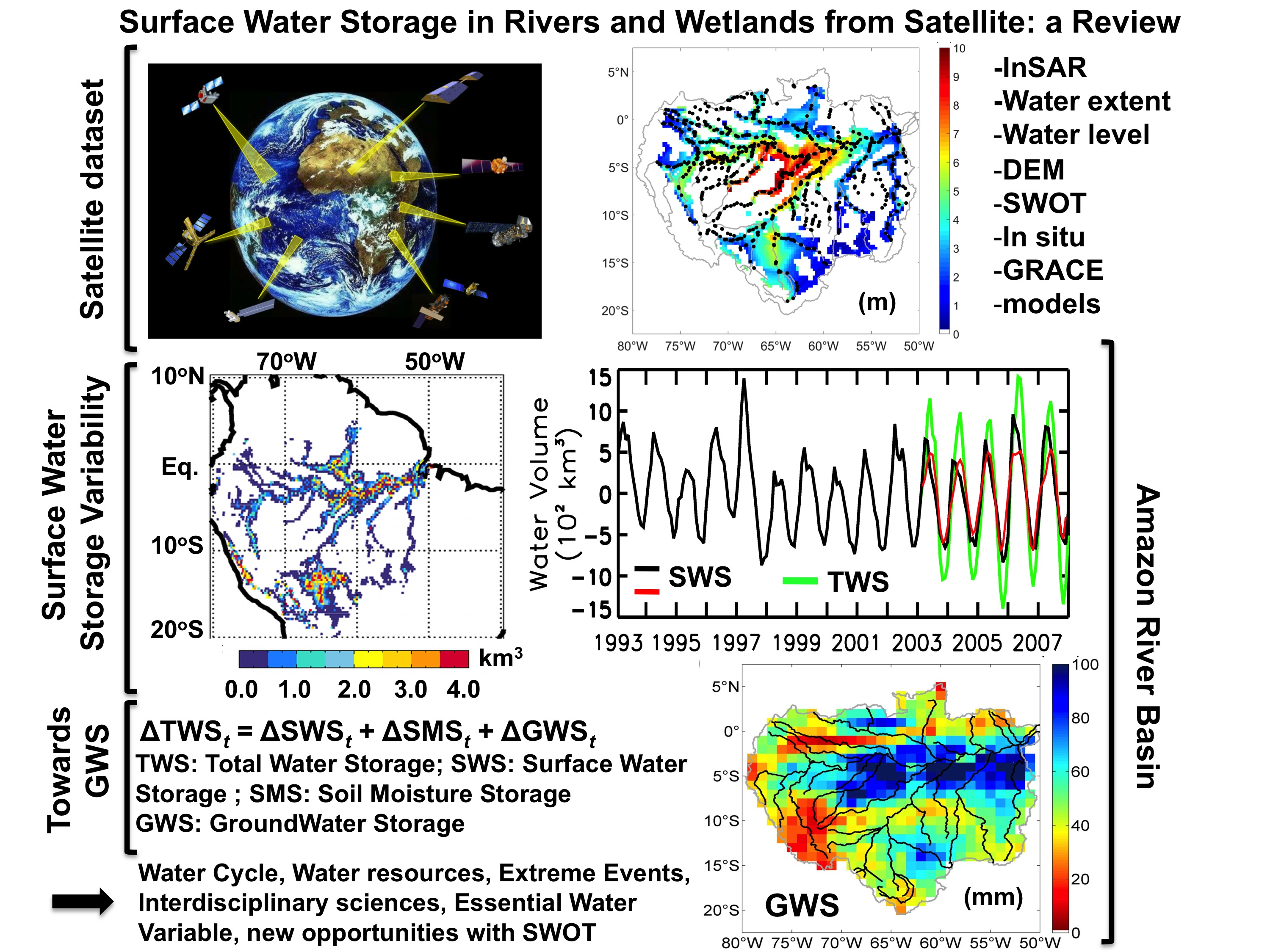
3.1. Estimates with SAR Interferometry (InSAR)

SAR interferometry (InSAR) consists of determining the phase differences of two or more complex SAR images (single look complex—SLC) acquired from a different angle and/or at different times [92]. It is a multiplicative interferometry technique, based on the product of one image by the complex conjugate of the second one or coherent cross-multiplication, allowing the retrieval of the difference of phase between the two signals. Changes in water level (dh) can be derived from the interferometric phase difference (Φ) [93].

dh = −λΦ/(4πcos θ) + n,

(3)

where λ is the wavelength of the electromagnetic wave emitted by the SAR sensor, θ is its incidence angle, and n is the noise caused by the decorrelation effect.

The quality of the interferogram is provided by the coherence, which represents the temporal similarity of any pixel between the SAR acquisitions. Loss of coherence or decorrelation is mostly due to three main factors: the difference in geometry due to the look angles of the satellite, volumetric decorrelation due to volumetric scattering of the vegetation, and temporal decorrelation related to changes in the scattering characteristic caused by changes in roughness and moisture content (e.g., variations of the leaf orientations, phenological cycle, and flood levels) [94]. The interferogram enables the determination of relative distances as a fraction of the radar wavelength. The difference in the sensor locations causes angular differences which are necessary for topographic mapping [95]. Different interferometry configurations (e.g., across-track, along-track, repeat-pass) allow a wide range of applications including topography, ice flow monitoring, crustal displacements, and subsidence, as well as water levels in wetlands and floodplains. This latter application is facing a large number of challenges due to the low backscattering of water surfaces [96] and the rapid variations in surface water conditions causing substantial changes in the backscattering [97]. For calm weather conditions, open water exhibits a smooth surface acting as a mirror for the electromagnetic (EM) wave emitted by the SAR in the microwave domain. The energy is mostly scattered away from the sensor, resulting in open water appearing dark in SAR images [96]. On the contrary, when the atmosphere is turbulent, open water presents a rougher surface with respect to the wavelength of the EM wave resulting in the backscattering of a part of the energy reaching the surface. In general, InSAR-derived water-level estimates are, before the launch of SWOT, based on the repeat-pass technique, the roughness of the water surface being very different from the time of acquisition of a SAR image to another, causing a loss of coherence between the two images [98]. Nevertheless, InSAR can be used for monitoring water levels under vegetation owing to the double-bounce effect. This mechanism consists of the backscattering caused by the vegetation after a reflection on the water surface (or the opposite) responsible for a backscattering enhancement compared with the case of open water. It was first identified and described by [99] and has been widely used to monitor flooded areas under vegetation (see [80] for a detailed review of the technique). The main characteristics of the SAR missions operating in InSAR mode mentioned below are presented in

Table 1. Main characteristics of SAR missions used in InSAR mode for SWS estimates. The first column gives the name of the space mission. The second column is the frequency of operation with the frequency band in brackets. The third and fourth columns provide the spatial and temporal resolutions of the data. The fifth column provides the period of data collection.

Sensor	Frequency in GHz (Band)	Polarization	Spatial Resolution (m)	Temporal Resolution	Period of Data Collection
Shuttle Imaging Radar with Payload C/X-SAR (SIR-C/X)	1.25 (L) 5.3 (C) 9.6 (X)	HH + HV + VH + VV (L and C) VV (X)	30 (L and C) 25 (X)		11–20 April 1994 30 September–11 October 1994
Japan Earth Resources Satellite (JERS-1)	1.275 (L)	HH	250	44 days	February 1992–November 1998
Phased array L-band synthetic aperture radar (PALSAR)	1.27 (L)	HH or VV	100 (ScanSAR)	46 days	January 2006–May 2011
Phased array L-band synthetic aperture radar-2 (PALSAR-2)	1.27 (L)	HH or VV or HV HH + HV or VH + VV	100 (ScanSAR)	14 days	Since November 2014

.

A first application of the InSAR technique was achieved on extensive floodplains of the Amazon Basin along a Shuttle Imaging Radar with Payload C/X-SAR (SIR-C/X) swath using L-band acquisitions at HH polarization, an incidence angle of 35° on two consecutive days, 9 and 10 October 1994, with a centimetric level of accuracy [100]. A decrease in water stage of 0.11 m was observed between the two consecutive days at a distance lower than 20 km of the main river, ranging between 0.02 and 0.05 m between 20 and 80 km. A more complete analysis was performed using all the acquisitions made at C and L bands for different polarizations (i.e., L-HH, L-HV, C-HH, and C-HV) [101]. Enhanced backscattering caused by the double bounce was observed at L and C bands in HH polarization over the margins of open water areas where shrubs and small trees were growing [102,103]. Strong temporal decorrelation (i.e., low coherence) was observed over open water [93,98,101]. Higher coherence was obtained at L- compared to at C-band over forested regions, as well as over flooded vegetation when using HH polarization rather than HV [93]. C- and X-bands, due to their lower penetration depth, are better suited for water detection over low vegetation such as herbaceous regions, whereas L-band needs to be used over woody wetlands [104,105]. Better accuracy was found when using SAR images at X- and C-bands rather than at L-band [106], but they had a lower range of level change that could be detected between two acquisitions due to a higher fringe saturation as their wavelength was smaller [107]. HH polarization was found to be more sensitive to the double-bounce effect over wetlands covered with vegetation rather than the other polarization, as the signal at HH polarization was less attenuated by the vegetation [108]. However, images acquired at VV polarization can be used to retrieve water-level changes during early stages of vegetation growth when the canopy is not well developed [107]. Nevertheless, images acquired at HV cross-polarization can reach a similar level of coherence than HH and VV co-polarizations but over shorter timespans [107,109].

Most of the studies cited above were either achieved over small wetlands as in Louisiana or in Florida or, over a short time period, over the Amazon. Very few studies used this promising technique to provide long-term monitoring of extensive wetlands in large river basins. The Japan Earth Resources Satellite-1 (JERS-1) L-band SAR acquisitions at 250 m of spatial resolution were used to estimate changes in water levels that occurred between 28 February 1993 and 11 April 1993 (mid-rising) and 15 April 1996 and 12 July 1996 (high water) in a region of ~100 km × 100 km of the central Amazon. Changes in water levels of several meters were recorded in good agreement with water levels measured at the in-situ gauges [110], as shown in Figure 1a. A similar study was performed using 6/6 SAR images acquired at L-band by PALSAR/PALSAR-2 in 2010 and 2015 at 100 m of spatial resolution, over a 3° × 3° region located in the upstream part of the Amazon Basin, at the junction of the mainstem, the Japura, and the Jurua rivers. Comparisons made against timeseries of water levels derived from the Satellite with Argos and Altika (SARAL) altimetry mission showed a good agreement with R² between 0.6 and 0.9 and RMSE lower than 0.2 m [111]. Water-level changes in the Tonle Sap basin, a sub-catchment of the Mekong basin in southeast Asia, were also estimated using six PALSAR images acquired in 2007. A good agreement was found when comparing the results from InSAR and radar altimetry from ENVISAT in terms of amplitude of the seasonal cycle [112]. The complementarity between InSAR and radar altimetry to derive SWS was more deeply exploited in the Congo Basin in two studies achieved in the extensive wetlands covering the Cuvette Centrale wetland. A first study used along-track profiles of radar altimetry data from ENVISAT to validate surface water-level estimates made using PALSAR images acquired from 2007 to 2010. Very good agreement was found with RMSE lower than 0.18 cm [113].

InSAR acquisitions from PALSAR allowed the establishment of a relationship between water depth (Figure 1b) and SWS from 2006–2011 over the Cuvette Centrale of Congo. This relationship was combined with ENVISAT data to level the SWS estimates over the whole study area from 2002–2011 [114]. A good agreement between dh/dt from InSAR and radar altimetry was observed considering several transects along the altimetry ground tracks, with RMSE varying from 0.1 to 0.22 m and R² ranging from 0.41 and 0.92. The InSAR technique is also used to study the hydrologic connectivity between the river and the floodplain and SWS changes, such as in the Ciénaga Grande de Santa Marta wetland located at the mouth of the Magdalena River (Colombia). Using 29 PALSAR images from 2006–2011, a characterization of the exchange between the floodplain and the river was achieved depending on the input flow of the river [115].

3.2. Multi-Satellite Approaches

Multi-satellite approaches to derive SWS are generally based on the complementarity between satellite images, which provide the spatiotemporal dynamics of the surface water extent, and satellite measurements of surface water elevation over inland water bodies (lakes, reservoirs, rivers, floodplains, and wetlands), generally obtained from radar altimetry. Thus, their combination offers the possibility to estimate SWS changes and water volume variations. All types of inundation extent product can be considered, from high- to moderate-spatial-resolution products, such as the dual-season mapping of wetland inundation and vegetation from the L-band SAR images acquired by JERS-1 at 100 m of spatial resolution [116], to global inundation products such as the Global Inundation Extent Multi-Satellite (hereafter GIEMS) [84,117].

Table 2 summarizes the major characteristics of the methodologies developed to estimate SWS as mentioned in this review.

A large number of radar altimetry-based timeseries of water level are necessary to adequately sample the hydrological variations in the watershed. The number of VS available is highly dependent on the orbit of the altimetric mission and on the shape of the rivers and associated floodplains in the area of interest. Radar altimetry missions such as ERS-2 (1995–2003), ENVISAT (2002–2010), and SARAL (2013–2016), with a repeat period of 35 days and an intertrack at the equator of ~80 km, as well as Sentinel-3A (since 2016) and Sentinel-3B (since 2018), with a repeat period of 27 days and an intertrack of 110 km, provide a much denser spatial sampling than the missions on an orbit with a 10 day repeat cycle and an intertrack at the equator of 315 km (such as Topex/Poseidon (1992–2002), Jason-1 (2002–2009), Jason-2 (2002–2016), Jason-3 (2016–present), and Sentinel-6A/Jason-CS (since 2020)). Examples of the use of multi-mission altimetry, covering various spatial and temporal coverages, are provided in several studies for various environments [118,119]. The VS timeseries can either be obtained from global databases (e.g., Hydroweb [120], DAHITI [121]) or be manually produced using dedicated software such as the Multi-Mission Altimetry Processing Software (MAPS) [118] or the Altimetry Time Series (AlTiS) [122].

A pioneering work was achieved in the Negro River Basin (~700,000 km²), the largest tributary to the Amazon in terms of discharge [123], combining a classification based on the dual-season mosaic from JERS-1 that discriminates open water, permanent, and temporary inundated areas from non-flooded zones and 88 VS (34 on the rivers and 54 on the floodplains) obtained at the cross-sections of the Topex/Poseidon (T/P) ground tracks with the rivers and floodplains [124]. Two maps of water level were computed during the low- and high-water stages, interpolated over the flood extent of September–December 1995 and May–July 1996, using the minimum/maximum of water levels recorded by each VS, with a time sampling of 10 days. From these maps, the maximum variation of SWS during the hydrological cycle was estimated. Yet, this first study had a strong limitation, since the use of the double mosaic did not allow monitoring the time variations of SWS. The authors of [125] then used a similar approach to estimate surface water volume change in the Mekong River basin. The methodology combined ERS-2, ENVISAT, and T/P satellite water-level timeseries along with monthly maps of surface water extent derived from daily multispectral images acquired by Satellite pour l’Observation de la Terre–Végétation (SPOT-VGT) at 1 km of spatial resolution [126]. The flood extent monitoring was limited to the months of flood occurrence (i.e., July to December) from 1998–2003. The monthly results helped characterize both the annual (with a peak in September or October) and the interannual (with the extreme flood of 2000) variabilities of water levels and SWS changes in the Lower Mekong Basin. However, the use of visible/near-infrared observations to detect the variations in surface water limits the development of the methodology to regions with low cloud cover and/or low vegetation cover [82].

A more robust methodology was then developed using surface water extent observations from the GIEMS multi-satellite technique [84,85,117] that captures the monthly extent of episodic and seasonal inundation, wetlands, rivers, and irrigated agriculture at the global scale at ~25 km of resolution and provides the percentage of inundation in a pixel of 773 km². The GIEMS technique is based on a joint use of a complementary suite of satellite observations covering a large wavelength range, mainly based on passive microwave emissivities, allowing the detection of water bodies under all weather conditions and vegetation covers. The spatiotemporal distribution and variability of GIEMS were extensively evaluated for various environments, including over the Amazon River basin, against high-resolution (100 m) SAR images [116], as well as using other regional surveys representing various components of wetland and open-water distributions. The evaluation led to an overall estimation of GIEMS uncertainties of ~10% [84].

The use of GIEMS monthly inundation extent in combination with satellite altimetry derived water levels to retrieve SWS was first developed over a tropical humid environment, covered with vegetation. Monthly maps of surface water levels and changes in surface water storage [127] were, thus, produced in the Negro River using 88 VS on the ground tracks of the nominal orbit of T/P mission from 1993–2000. A similar approach [128] was then tested with success over a totally different environment, the Lower Ob’ region (~512,000 km²), an Arctic River located in Boreal Russia, dominated by seasonal snow and ice cover, using an altimetry-based hydrological network of Topex/Poseidon VS (90 VS for the nominal orbit 1993–2002 and 92 for the interleaved new orbit 2002–2004). These two preliminary studies showed the large potential of the methodology, which can be applied to tropical and to boreal environments.

The results in the Negro River Basin were further extended to a 2 year period (2003–2004) combining GIEMS with 140 VS under the ENVISAT ground tracks. Additionally, in this new study, the monthly maps of surface water levels were referenced for the first time to a map of minimum water levels estimated during the entire observation period based on hypsometric curves [129]. The hypsometric approach helps account for the difference of elevations between the river and the floodplain in each GIEMS pixel. Details on hypsometric curves are provided in Section 3.3.

This enabled the development of the methodology over the entire Amazon River basin [130] using hundreds of altimetry-derived water levels over floodplains and wetlands. Here, we summarize the methodology as illustrated in [70,130]. Firstly, using continuous water-level observations derived from the ENVISAT radar altimeter (between 2003 and 2010 for instance) along with GIEMS observations, monthly surface water-level maps can be obtained using a bilinear interpolation. Each monthly map of surface water levels has a spatial resolution of 0.25° and is referenced to the EGM2008 geoid. Figure 2 illustrates the main characteristics of GIEMS surface water extent over the Amazon along with the location of the ~900 RA-2 altimetry VS and shows the map of mean water level from 2003–2010 over the entire basin.

A map of minimum water levels is also estimated for the entire observation period using a hypsometric approach to take into account the difference in altitude between the river and the floodplain. Second, surface water volume variations for the Amazon River are estimated using the surface water-level maps. At the basin scale, the time variations of SWS are computed as

$$V_{SW}\left(t\right)=R_e^2{\displaystyle \sum }_{j\in S}P\left({\lambda }_j,{\phi }_j,t\right)(h\left({\lambda }_j,{\phi }_j,t\right)-h_{min}\left({\lambda }_j,{\phi }_j\right))\cos \left({\phi }_j\right)\Delta \lambda \Delta \phi$$

(4)

where V_SW is the volume of surface water, R_e is the radius of the Earth (6378 km), P(λ_j,φ_j,t), h(λ_j,φ_j,t), and h_min(λ_j,φ_j) are, respectively, the percentage of inundation, the water level at time t, and the minimum of water level at the pixel (λ_j,φ_j), and Δλ and Δφ are, respectively, the grid steps in longitude and latitude. The minimum water level is estimated through a hypsometric approach relating the percentage of inundation of a pixel to its elevation. A maximum error on the volume variation is estimated as follows:

$$\Delta V_{SW,max}\le \Delta S_{max}\delta h_{max}+S_{max}\Delta \left(\delta h_{max}\right)$$

(5)

where ΔV_SW,max is the maximum error on the water monthly volume anomaly, S_max is the maximum monthly flooded surface, δh_max is the maximum water-level variation between two consecutive months, ΔS_max is the maximum error for the flooded surface, and Δ(δh_max) is the maximum error for the water level between two consecutive months.

The combination of GIEMS surface water extent with ENVISAT-derived water-level variations was later applied to the largest world drainage basins, during the period of common availability of both datasets (2003–2007), in order to estimate the pluriannual variations of the amount of freshwater stored in floodplains, rivers, and wetlands: the Orinoco [131], the Ganges–Brahmaputra [132], and the Congo River basin [133]. For the Amazon Basin, the first estimates were then extended until 2010 (the end of data acquisition for ENVISAT on its nominal orbit) using the mean annual cycle of GIEMS after 2007 [70]. Following a similar approach, Ref. [134] combined water-level timeseries at 187 ENVISAT VS distributed over the entire Amazon basin, together with the surface water extent variations from GIEMS to derive SWS from 2003 to 2007.

One of the limitations of the combination of GIEMS and radar altimeter observations lies in the fact that concurrent observations are needed, often limiting the length of the timeseries [129]. In order to obtain longer timeseries of surface water storage, methodologies combining timeseries of water levels from ERS-2, ENVISAT, and SARAL altimetric missions were further applied to Moderate Resolution Imaging Spectroradiometer (MODIS)-based inundation extent, offering observations from 2000. These inundation extents are generally derived from the 8 day synthesis of MODIS surface reflectance at 500 m spatial resolution using a simplified version of the decision-tree based on thresholds of the enhanced vegetation index (EVI [135]), land surface water index (LSWI [136]), and their difference [137]. SWS of the Tonle Sap Basin (part of the lower Mekong basin) was estimated from 1993–2016 [138], using the MODIS-derived surface water extent combined with altimetry-based water levels from multiple missions (T/P, Jason-1, 2, 3, ENVISAT, and SARAL). Similarly, using MODIS-based surface water extent maps and 45 VS from ENVISAT, monthly maps of water level and SWS were generated in the Lower Mekong Basin from 2003–2010 [139]. Compared to SPOT-VGT (1 km from blue to near-infrared) used in [125], MODIS-derived inundations help monitor the changes during the entire hydrological cycle [138,139], thanks to a better spatial resolution (500 m) and a larger number of spectral bands ranging from blue to shortwave infrared (SWIR). A similar approach was also applied to monitor SWS changes in an Arctic environment, the McKenzie Delta (13,135 km²) in the north of Canada, using water levels from ERS-2 (22 VS), ENVISAT (27 VS), and SARAL (24 VS), covering a period of more than 15 years from 2000 to 2015 [140]. As this region is located between 67° N and 70° N, the delta is seasonally covered with snow and ice, such that SWS estimates are limited to the ice-free period from June to September. A similar methodology, based on the complementary use of MODIS-derived surface water extent and multi-mission satellite altimetry observations (from T/P, Jason-1, 2, 3, ENVISAT, and SARAL), was then applied to estimate the variations in SWS for the last two decades (2000–2019) over the Lake Chad watershed in Africa, including its seasonal adjacent wetlands covered by vegetation [141].

Another approach to estimate SWS is to solve the water balance equation combining various remotely sensed observations (i.e., GRACE, radar altimetry, rainfall from Global Precipitation Climatology Project—GPCP, SRTM DEM, SAR (JERS-1), and multispectral (MODIS) images). This approach was applied to the Amazon and Congo floodplains, respectively [142,143].

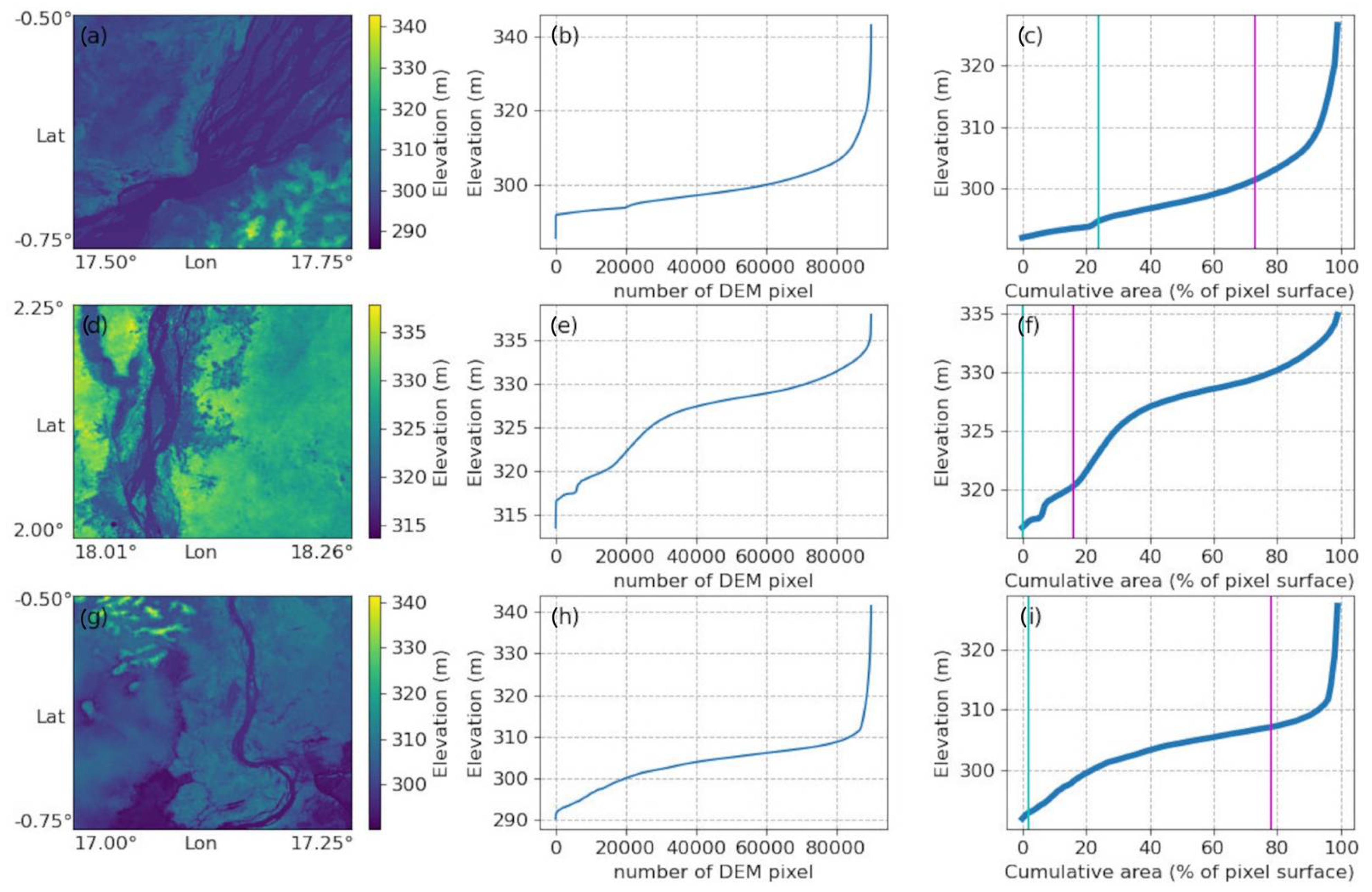
3.3. Hypsometric Curve Approach Using Digital Elevation Models

In parallel to the use of multi-satellite approach methodologies, combining paired water-level and water-extent observations (Section 3.2) to estimate SWS, techniques based on the relationships between elevation and surface area variations, called the hypsometry approach, were also developed.

The relationships among the area or extent, the depth, and the volume of water in topographic depressions such as lakes, wetlands, and floodplains have long been used to study water and dissolved-mass balances in these hydrological systems [144,145]. The area–elevation–volume relationship is usually obtained from fine-resolution elevation maps and data that help to quantify the filling and spilling of the change of water volume in the topographic depressions, which often are site-specific by nature [146].

At larger scale, the concept of the hypsometry approach to estimate SWS was further developed for lakes and reservoirs thanks to the advances in radar altimetry measurements. As stated in Section 1, the present review does not deal with SWS variations in lakes and manmade reservoirs and, for this specific topic, we refer to other publications and reviews [88,89,90,91,147]. Several databases that provide such estimates [148,149] are now available. Notably, Ref. [91] estimated continuous and global surface water storage changes in large lakes and reservoirs for 1992–2019, building on relationships between elevation and surface area from multiple satellite altimetry missions (TOPEX-Poseidon, Jason-1, 2, 3, and ENVISAT) and surface extent estimated from Terra/Aqua MODIS, producing estimates even during periods when either of the variables was not available.

At the scale of large river basins, the use of DEM in the development of the hypsometry approach to estimate SWS was then motivated by the fact that the variations in the storage and movement of surface water were not realistically represented in continental- to global-scale river routing models [41]. Indeed, until recently, river channel and floodplain inundation dynamics were not considered in large-scale river routing models because surface water characteristics are generally regulated by small-scale topography rather that could not be represented by the coarse spatial resolution of global hydrological models. With the advent of global and fine-resolution (≤1 km) DEMs from space, such as Shuttle Radar Topography Mission (SRTM, 90 m), Advanced Spaceborne Thermal Emission and Reflection Radiometer Global Digital Elevation Model (ASTER GDEM, 30 m), or Multi-Error-Removed Improved-Terrain DEM (MERIT DEM, 90 m, derived from SRTM), more detailed observations are available to explain surface water dynamics in continental-scale rivers [150]. Using these global DEM datasets, hydrography maps giving fine-resolution flow direction, such as HydroSHEDS (90 m), HYDRO1k (1 km), and MERIT-Hydro, can be obtained [151,152], and they are commonly used in river routing models for explicitly simulating inundation dynamics in small basins [153,154]. With a better resolved terrain surface, the representation of surface water depth and inundated area for large-scale models was then introduced using the detailed topography of river channels and floodplains to estimate water stage variation on the subgrid scale. The authors of [66,155] firstly calculated the relationship between water volume and flooded area using subgrid topography for the explicit prediction of inundated area, demonstrating an improved estimate of river discharge in the Amazon. The authors of [41] further improved these approaches describing the relationship among water volume, flooded area, and river stage in river channel and floodplain in the Catchment-Based Macroscale Floodplain (CaMa-Flood) model, using subgrid-scale topography at 1 km resolution of floodplains. The cumulative distribution function of the elevation within each CaMa-Flood unit catchment was derived to describe the floodplain elevation profile as a function of the flooded area fraction and the floodplain water depth, under the assumptions that (1) the river channel and floodplain are seen as continuous reservoirs, in that water spilling from the river channel is stored in the floodplain, assuming polygonal storages for river channels and floodplains, and (2) inundation occurs from lower to higher areas within the model unit catchment. These advances were then implemented in other hydrological models [156,157].

On the basis of similar approaches to that developed for large-scale models, innovative observation-based methodologies were proposed using a hypsographic curve technique to estimate SWS variations, combining surface water extent from satellite observations with topographic data from DEM. For instance, Ref. [78] used the Global Digital Elevation Model (GDEM) from Advanced Spaceborne Thermal Emission and Reflection Radiometer (ASTER), ASTER-GDEM [158], in combination with the surface water extent from GIEMS, to estimate surface freshwater storage variations in rivers, floodplains, and wetlands of the Amazon River basin from 1993 to 2007. While the methodology can be applied to various satellite-derived surface water extent products combined with any large-scale and high-resolution DEM, here, we use the example of the combination of GIEMS and MERIT DEM at 90 m over the Congo basin to briefly describe the methodology. It is a three-step process that can be summarized as follows: (1) for each cell of the GIEMS dataset (on an equal-area grid of 0.25° at the equator of 773 km²), the cumulative distribution function of elevation values is first derived from the corresponding subset of MERIT DEM (Figure 3, right). Over the Congo basin, this corresponds to ~95,000 elevation points falling within the satellite-derived surface water extent cell, from which the so-called hypsographic curve or curve of cumulative frequencies is constructed, equivalent to the distribution of elevation values in each 773 km² cell sorted in ascending order to represent an area–elevation relationship (Figure 3, middle); (2) the hypsographic curve of the area–elevation relationship (Figure 3, right) is converted into an area–surface water volume relationship by estimating the surface water volume associated with an increase of the pixel fractional open water coverage (generally 1%) by filling the hypsographic curve from its base level to an upward level; (3) the hypsographic curve of the area–surface water volume relationship obtained is combined with the monthly variations in surface water extent from GIEMS to estimate the surface water volume for each month by intersecting the hypsographic curve value with the GIEMS estimates of pixel water coverage for that month. Note that, with the proposed method, the water storages below the lowest levels of storage are not accessible; thus, the estimated water storage represents the increment above the minimum observed storage. We also refer to Figure 6 of [78] and Figure 4 of [159] for a complete illustration of the three-step methodology.

SWS estimates using the hypsometry approach were derived over the entire Amazon River basin [78] using ASTER GDEM combined with GIEMS. SWS estimates were then produced for the Ganges–Brahmaputra River basin, including the deltaic region located in Bangladesh [159] using two different sets of hypsometric curves derived from ASTER GDEM and modulated SRTM30 DEM [160,161]. Since GIEMS and DEMs are available globally, these attempts are promising steps toward the development of SWS estimates at the global scale. Other surface water-extent datasets which provide the fractional extent of water, such as Surface Water Microwave Product Series (SWAMPS) [86] or the SMOS-based product named SWAF [162] could also be used.

The use of global satellite-derived DEMs has some limitations and uncertainties that can cause significant problems or errors when used for hydrological applications, such as the estimations of SWS [78,160]. Typical errors and problems are generally related to the influence of vegetation, manmade constructions, or errors due to cloud cover (especially dense boundary layer clouds when using near-infrared spectral bands with ASTER GDEM). DEM errors remain as one of the main sources of uncertainty for understanding the interactions between rivers and floodplains, since, in low relief areas, small deviations from the true surface elevation can cause errors representing the river and floodplain profiles. Recently, the performance of DEMs for hydrological applications have been improved, particularly with the release of MERIT DEM [163] and ALOS World 3D from JAXA at 30 m spatial resolution (AW3D30) [164]. Their use to retrieve SWS should be investigated in the future, with the aim of representation at the global scale.

Using in situ Amazon River water levels and a flood-frequency map derived from the Landsat Global Surface Water Dataset [83], a 30 m high-resolution topographic mapping of the middle–lower Amazon floodplain for its non-forested portion was generated and further used to derive floodplain depths and estimate SWS changes in open-water floodplains [83,165].

Table 2. Main characteristics of the various approaches used to estimate SWS variations across studies for several large river basins. The first column is the name of the river basin. The second column is the total drainage area of the basin, and the value in brackets is the area considered for the cited study. The third column provides the method used to derive SWS along with the references of the study in brackets. The fourth and fifth columns provide the spatial and temporal resolutions of the SWS estimates. The sixth column provides the time span of the dataset.

River Basin or Sub-Basin	Area (km2)	Method	Spatial Resolution	Temporal Resolution	Time Span
Amazon	6.0 million	GIEMS + altimetry [70,130]	0.25°	Monthly	2003–2010, 2003–2007
		hypsometric curve [78]	0.25°	Monthly	1993–2007
		GIEMS + altimetry [134]			2002–2007
Congo	3.7 million	GIEMS + altimetry [133]	0.25°	Monthly	2003–2007
Ganges–Brahmaputra	1.7 million	GIEMS + altimetry [132]	0.25°	Monthly	2003–2007
		Hypsometric curve (ASTER-based) [159]	0.25°	Monthly	1993–2007
		Hypsometric curve (Hymap-based) [159]	0.25°	Monthly	1993–2007
Orinoco	1.0 million	GIEMS + altimetry [131]	0.25°	Monthly	2003–2007
Mekong (lower)	800,000 (~100,000)	MODIS + altimetry [138]	500 m	10 days	2003–2009
		SPOT-VGT + altimetry [125]	1 km	Monthly	1998–2003
Tonle Sap (Lower Mekong)	86,000	MODIS + altimetry [138]	500 m	Monthly	1993–2017
Ob (lower)	2.7 million (~512,000)	GIEMS + altimetry [128]	0.25°	Monthly	1993–2004
MacKenzie (delta)	1.8 million (13,000)	MODIS + altimetry [140]	500 m	10 days	2000–2015
Chad (lake and wetlands)	2.6 million (~20,000)	MODIS + altimetry [141]	500 m	10 days	2003–2018
Rio Negro (Amazon sub-basin)	700,000	GIEMS + altimetry [127]	0.25°	Monthly	2003–2004
		JERS-1 + altimetry [124]	100 m	Two dates	1995–1996
Amazon main stem	6 tiles of 300 × 300 km	(Tile ranging from 25 to 80), water balance equation with multiple satellites [142]	300 km	15 days	July 2003–June 2006
Non-forested floodplain in the middle–lower Amazon	1.5° of latitude × 8° of longitude	water levels and a flood-frequency map [165]	30 m	Static	1984–2015
Congo (central)	3 tiles of 300 × 300 km	water balance equation with multiple satellites [143]	3°	Monthly	2003–2008
Congo (central, flooded forests)	1 tile 350 km × 350 km	PALSAR + MODIS [111]	250 m	4 dates	July 2007–September 2008
Congo (floodplains)	11 tiles 350 km × 350 km	PALSAR (InSAR) [113]	100 m	3 dates/path	July 2006–August 2010
Ganges (alone)	950,000	GIEMS + altimetry [132]	0.25°	Monthly	2003–2007
		hypsometric curve (ASTER-based) [159]	0.25°	Monthly	1993–2007
		hypsometric curve (HyMap-based) [159]	0.25°	Monthly	1993–2007
Brahmaputra (alone)	850,000	GIEMS + altimetry [130]	0.25°	Monthly	2003–2007
		hypsometric curve (ASTER-based) [159]	0.25°	Monthly	1993–2007
		hypsometric curve (HyMap-based) [159]	0.25°	Monthly	1993–2007

Table 2. Main characteristics of the various approaches used to estimate SWS variations across studies for several large river basins. The first column is the name of the river basin. The second column is the total drainage area of the basin, and the value in brackets is the area considered for the cited study. The third column provides the method used to derive SWS along with the references of the study in brackets. The fourth and fifth columns provide the spatial and temporal resolutions of the SWS estimates. The sixth column provides the time span of the dataset.

River Basin or Sub-Basin	Area (km2)	Method	Spatial Resolution	Temporal Resolution	Time Span
Amazon	6.0 million	GIEMS + altimetry [70,130]	0.25°	Monthly	2003–2010, 2003–2007
		hypsometric curve [78]	0.25°	Monthly	1993–2007
		GIEMS + altimetry [134]			2002–2007
Congo	3.7 million	GIEMS + altimetry [133]	0.25°	Monthly	2003–2007
Ganges–Brahmaputra	1.7 million	GIEMS + altimetry [132]	0.25°	Monthly	2003–2007
		Hypsometric curve (ASTER-based) [159]	0.25°	Monthly	1993–2007
		Hypsometric curve (Hymap-based) [159]	0.25°	Monthly	1993–2007
Orinoco	1.0 million	GIEMS + altimetry [131]	0.25°	Monthly	2003–2007
Mekong (lower)	800,000 (~100,000)	MODIS + altimetry [138]	500 m	10 days	2003–2009
		SPOT-VGT + altimetry [125]	1 km	Monthly	1998–2003
Tonle Sap (Lower Mekong)	86,000	MODIS + altimetry [138]	500 m	Monthly	1993–2017
Ob (lower)	2.7 million (~512,000)	GIEMS + altimetry [128]	0.25°	Monthly	1993–2004
MacKenzie (delta)	1.8 million (13,000)	MODIS + altimetry [140]	500 m	10 days	2000–2015
Chad (lake and wetlands)	2.6 million (~20,000)	MODIS + altimetry [141]	500 m	10 days	2003–2018
Rio Negro (Amazon sub-basin)	700,000	GIEMS + altimetry [127]	0.25°	Monthly	2003–2004
		JERS-1 + altimetry [124]	100 m	Two dates	1995–1996
Amazon main stem	6 tiles of 300 × 300 km	(Tile ranging from 25 to 80), water balance equation with multiple satellites [142]	300 km	15 days	July 2003–June 2006
Non-forested floodplain in the middle–lower Amazon	1.5° of latitude × 8° of longitude	water levels and a flood-frequency map [165]	30 m	Static	1984–2015
Congo (central)	3 tiles of 300 × 300 km	water balance equation with multiple satellites [143]	3°	Monthly	2003–2008
Congo (central, flooded forests)	1 tile 350 km × 350 km	PALSAR + MODIS [111]	250 m	4 dates	July 2007–September 2008
Congo (floodplains)	11 tiles 350 km × 350 km	PALSAR (InSAR) [113]	100 m	3 dates/path	July 2006–August 2010
Ganges (alone)	950,000	GIEMS + altimetry [132]	0.25°	Monthly	2003–2007
		hypsometric curve (ASTER-based) [159]	0.25°	Monthly	1993–2007
		hypsometric curve (HyMap-based) [159]	0.25°	Monthly	1993–2007
Brahmaputra (alone)	850,000	GIEMS + altimetry [130]	0.25°	Monthly	2003–2007
		hypsometric curve (ASTER-based) [159]	0.25°	Monthly	1993–2007
		hypsometric curve (HyMap-based) [159]	0.25°	Monthly	1993–2007

4. Understanding the Dynamics of Surface Freshwater in Large Rivers

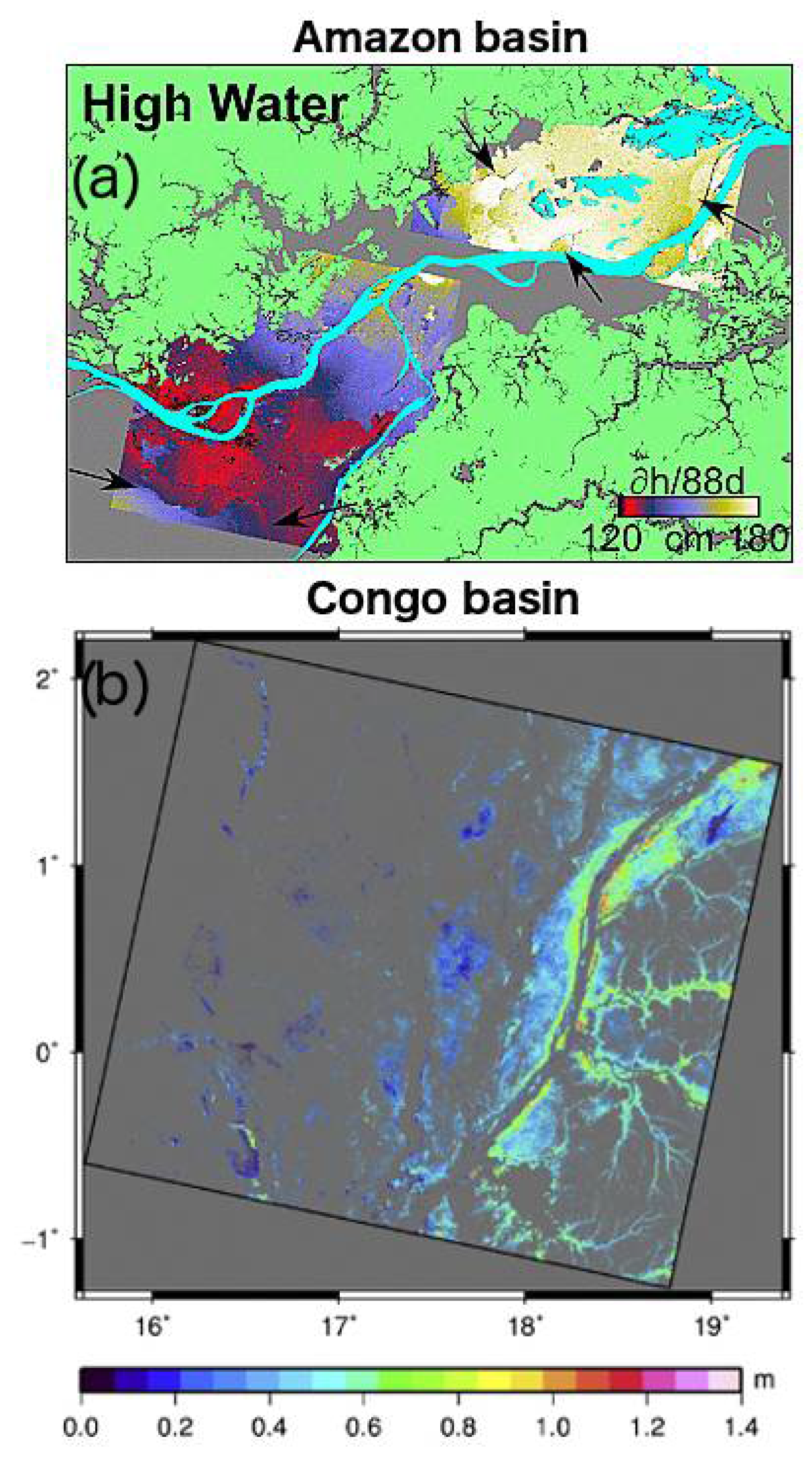
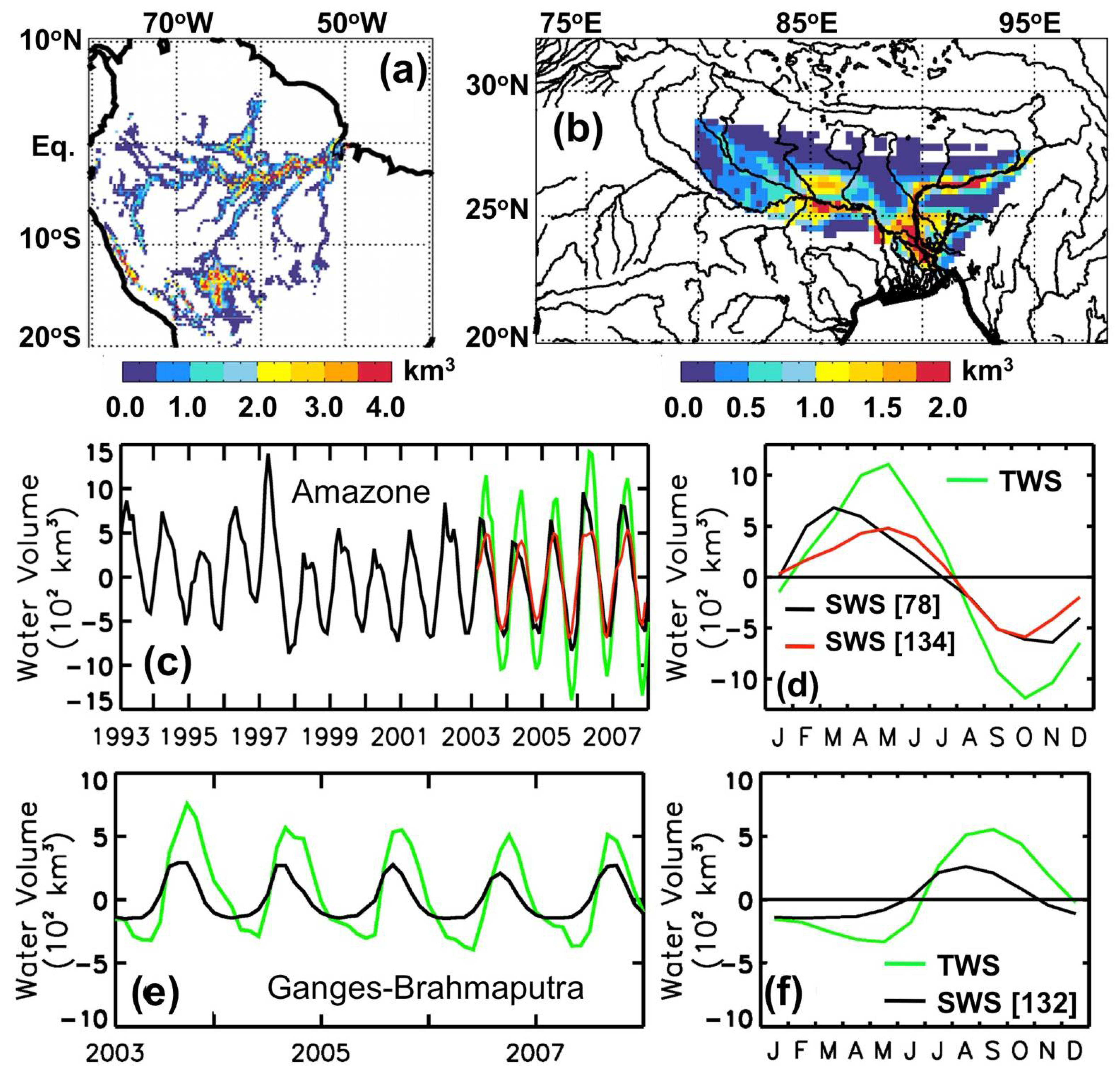
4.1. Seasonal Variations in SWS Change across Large River Basins

The new availability of satellite-based SWS databases fosters new understanding of the characterization and dynamics of surface water movement and surface hydrology in large river basins.

The Amazon River basin is the geographical region where the use of SWS new estimates enabled first scientific progress from local to basin scale, across several timescales. On the Uatuma River, the Balbina water includes a cluster of islands separated by submerged, shallow valleys within a flooded water surface area of 2400 m² where JERS-1 SAR-derived water height changes (∼12 cm) were, for the first time, converted to a net volume measurement (280 million m³) over the 44 days separating the satellite acquisitions, showing that, compared to historical gauge records, removal of this volume from the lake required a ∼50% greater flow [101]. Over a larger area, the Rio Negro sub-basin of the Amazon River, the maximum variation of surface water storage during the seasonal hydrological cycle of 1995–1996 was estimated at ~330 km³ [124], a first independent and unprecedented estimate that helped show that the storage capacity of the Rio Negro floodplain was not linearly related to the amount of water that flew from the basin. This absence of a relationship between water volume and inundated area was attributed to the diverse and widely dispersed floodplains of the basin. These estimates were found to be 30% larger than the surface water volume change estimated on a monthly basis for 1993–2000 [127], showing some consistency between GIEMS-based and SAR-based estimates, even if discrepancies were noted due to the differences in surface water extent between both techniques. Nevertheless, the changes in surface water storage compared well with rainfall estimates with large correlation, with a time lag found at the scale of Negro River Basin [127]. On the other hand, lower correlations with river discharge were observed, mainly attributed to the backwater effect from the Amazon main stem [123]. At the Amazon basin scale, first estimates of SWS annual variations from satellite observations were further provided with a mean annual amplitude ranging from ~900 km³ (mean over 2003–2007 [130]) to ~1200 km³ (mean over 1993–2007 [78]), which represents 20–30% of the water volume that flowed out of the Amazon basin. The authors of [70] provided SWS change annual amplitude for seven different Amazon sub-basins. The most important contributions to basin-scale SWS variations came from the Solimoes and the Madeira sub-basins (30% and 25%, respectively), whereas the contribution from the Tapajos represented less than 6% of the water stored in the surface reservoir of the Amazon basin.

The observation-based estimates are in the range of previous estimates from large-scale model simulations that reported a seasonal amplitude of ~1100 km³ using the Hydrological Modeling and Analysis Platform (HyMAP) model [161], which includes floodplain reservoirs, and further supported previous estimates [134] of the surface water volume variation of the Amazon basin ranging annually from −554 km³ to 662 km³ (1071 km³ of mean annual amplitude for the period 2003–2007). Amazon SWS estimates also show substantial variability at the interannual timescale, especially regarding annual maxima and minima, with extreme minima in the years 1997 and 2005, associated for instance with the major drought occurring during these periods (discussed in Section 4.2). These estimates over the Amazon are summarized in Figure 4a,c,d.

The SWS estimates over the Amazon were evaluated against other independent hydrological variables showing a strong correspondence against precipitation and in situ river discharge, often with a time-lag revealing how extensive floodplains first store and then release large amounts of water to the main rivers and, consequently, delay flood waves and alter water transport [166]. The 2 month delay between the maximum surface water volume and GRACE TWS annual peak also revealed the slower sub-surface and groundwater flow in comparison to the surface water movement [78,134,161]. Over the basin-wide Amazon, modeling studies suggest that channel and floodplain discharge account for 40% of the total change in the water balance as compared to changes in soil moisture and groundwater, which account for the remaining portions [167]. However, from observations, the amount of water on Amazon floodplains or the amount exchanged with adjacent channels is still poorly unknown, and only [142], who combined gravimetric and imaging satellite methods, estimated the amounts of water seasonally filling and draining from the mainstem Amazon floodplain, with regions of about 300 km × 300 km draining between 25 to 80 km³ of water each year (i.e., the range from maximum to minimum storage), amounting to 285 km³ in total. However, they demonstrated that these large floodplain volumes and fluxes are small compared to the discharge of the Amazon River, as floodplain volume estimates amount to about 5% of the total volume of water annually discharged from the Amazon. Over the open-water floodplains of the Amazon, Ref. [165] showed that SWS varies 104.3 km³ on average each year (from 11.9 km³ in low-water to 116.2 km³ in high-water stages).

Over the flooded forest in the central Congo Basin, SWS changes were calculated from water depth maps from InSAR and altimetry [113] to be 11.3 ± 2.0 km³, 10.3 ± 2.3 km³, and 9.3 ± 1.8 km³ for 12 May 2006, 12 August 2007, and 12 October 2008, respectively. From 2002–2011, an average annual SWS change of 3.86 ± 0.59 km³ was obtained over an inundated area of ~7800 km² [114]. Solving the water balance equation and using multi-satellite information including GRACE-based TWS, Ref. [143] found an annual amplitude of SWS of 111 km³. Following those advances over the Amazon, SWS estimates over other large river basins were obtained in various climatic environments, including the Ganges–Brahmaputra (Figure 4b,e,f). Over the MacKenzie delta, satellite-derived estimates [140] compared well with independent estimates from digital topographic maps and water levels [168]. The results of these various studies are summarized in

Table 3. Mean annual amplitudes of SWS variations estimated across studies for several large river basins. The first column is the name of the river basin. The second column is the total drainage area of the basin, and the value in brackets is the area considered for the cited study. The third column provides the estimates of mean annual amplitudes of SWS variations in km³, along with uncertainties when available. The method used is provided along with the references of the study in brackets.

River Basin or Sub-Basin	Area (km2)	SWS Change Mean Annual Amplitude (km3) ± Uncertainties
Amazon	6.0 million	900 ± 162, GIEMS + altimetry [70,130] 1200, hypsometric curve [78] 1071, GIEMS + altimetry [134]
Congo	3.7 million	~81 ± 24, GIEMS + altimetry [133]
Ganges–Brahmaputra	1.7 million	410 ± 96, GIEMS + altimetry [132] 496, hypsometric curve (ASTER-based) [159] 378, hypsometric curve (Hymap-based) [159]
Orinoco	1.0 million	170, GIEMS + altimetry [131]
Mekong (lower)	800,000 (~100,000)	40, MODIS + altimetry [139] 38.2 ± 16, SPOT-VGT + altimetry [125]
Tonle Sap (Lower Mekong)	86,000	31 to 101, MODIS + altimetry [137]
Ob (lower)	2.7 million (~512,000)	90, GIEMS + altimetry [127]
MacKenzie (delta)	1.8 million (13,000)	9.6, MODIS + altimetry [139]
Chad (lake and wetlands)	2.6 million (~20,000)	1.2, MODIS + altimetry [141]
Rio Negro (Amazon sub-basin)	700,000	167 ± 39, GIEMS + altimetry [127] 220, JERS-1 + altimetry [124]
Amazon main stem	6 tiles of 300 × 300 km	285 (tile ranging from 25 to 80), water balance equation with multiple satellites [142]
Non-forested floodplain in the middle–lower Amazon	/	104, water levels and a flood-frequency map [165]
Congo (central)	3 tiles of 300 × 300 km	111, water balance equation with multiple satellites [143]
Congo (central, flooded forests)	/	11.3 ± 2.0 (12 May 2006), 10.3 ± 2.3 (12 August 2007), 9.3 ± 1.8 (12 October 2008) [113]
Congo (floodplains)	7800 km2	3.86 ± 0.59 [114]
Ganges (alone)	950,000	300, GIEMS + altimetry [132] 496, hypsometric curve (ASTER-based) [159] 378, hypsometric curve (HyMap-based) [159]
Brahmaputra (alone)	850,000	250, GIEMS + altimetry [130] 254, hypsometric curve (ASTER-based) [159] 172, hypsometric curve (HyMap-based) [159]

, which provides the mean annual amplitudes of SWS variations estimated across studies and methods for several large river basins. These estimates, obtained from several independent methods (Section 3) generally compare well over a same river basin. These observations are powerful tools to study the complex dynamics of surface water in large drainage basins (i.e., backwater effects, flood-pulse, and time residence of water in the floodplains), providing unique and valuable spatial information on the time evolution of river, floodplain, and wetland reservoirs during the hydrological cycle in response to seasonal, interannual, and long-term variability.

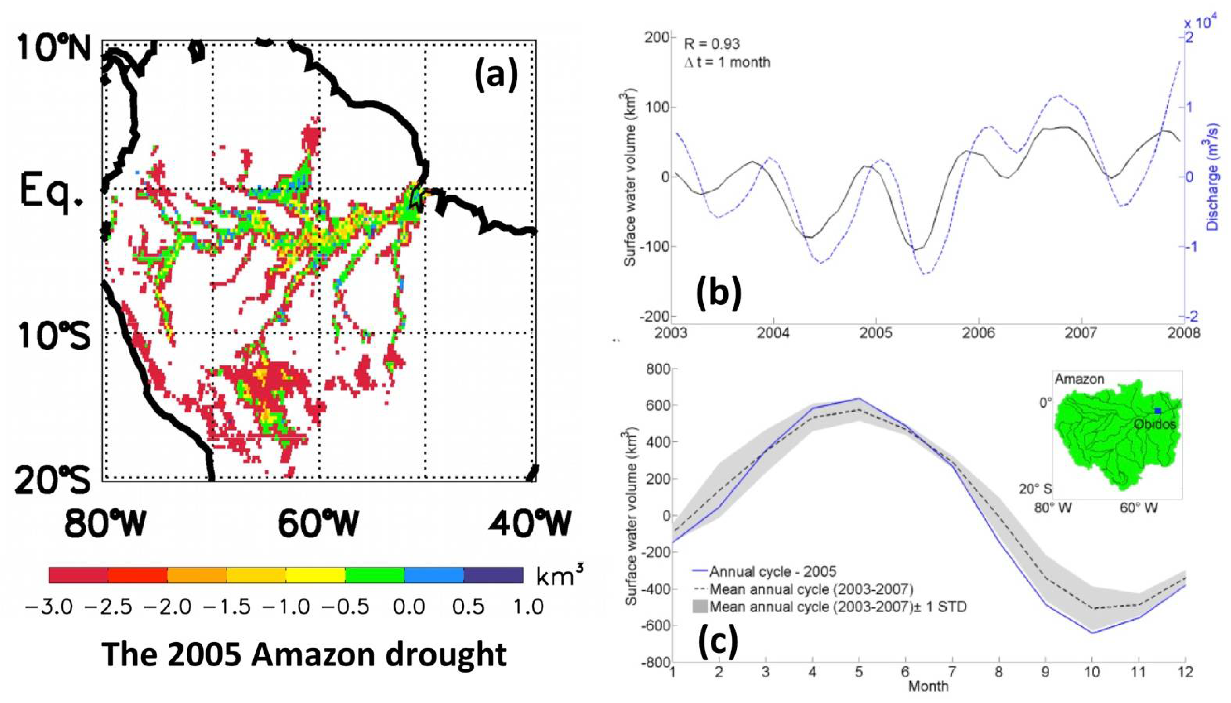
4.2. Quantifying Extreme Event Impacts on Surface Water Storage

In addition to the estimates of seasonal amplitude, the availability of SWS changes over several years now makes it possible to characterize the interannual variability of SWS, which, for large tropical basins, can be very large. For instance, over the Congo floodplains, Ref. [111] showed that the maximum water volume could vary from ~5.9 km³ in a wet year such as 2002 to a minimum volume of 2.01 km³ in a dry year such as 2005, with the interannual variability in SWS being mainly explained by the changes in precipitation. Large river basins, such as Congo, Ganges–Brahmaputra, and Amazon, also exhibit large interannual variability, with [78] reporting SWS annual changes over the 1993–2007 period ranging from ~800 to 1300 km³ over the Amazon. More interestingly, the availability of pluriannual SWS changes offer the possibility to quantify and spatialize the signatures of extreme event phenomena, such as large droughts and floods, directly from observations, as well as characterize their impacts on the dynamics of surface water. Here, we illustrate the signature of such events over the Amazon and the Ganges–Brahmaputra River basins, where datasets covering multiyear observations are available. Indeed, the droughts that affected large areas of the Amazon basin in recent years are amongst the most severe ones in the past hundred years [169] with the events in 1997–1998, 2005, and 2010 still considered as the most exceptional ones in the last 40 years.

Focusing on the signature of the 2005 drought on Amazon surface water (Figure 5), for the first time, Ref. [130] monitored and mapped the evolution of the surface water level and volume anomalies over the entire event for the whole basin. The reduction in rainfall over southern Amazonia since 2002 caused a decrease in water stored in the floodplains up to the minimum of 2005, also observed on stream flow (Figure 5).

While the annual cycle of surface water storage for 2005 was close to normal from February to June, it became significantly lower than the mean during the dry season from August until December. The impact of the 2005 drought was quantified for the surface water storage of the whole Amazon basin to be 129 km³ below its 2003–2007 average, such that the minimum volume of surface water stored in the entire basin was 71% lower that year. Spatial variabilities of SWS deficit at the sub-basin scale (−86% for the Solimoes and −66% for the Tapajos) were reported. These figures were later confirmed using observations over a longer time period, suggesting that, during the extreme droughts of 1997 (October–November) and 2005 (September–October), the water stored in the river and floodplains of the Amazon basin was, respectively, ~230 (~40%) and 210 (~50%) km³ below the 1993–2007 average [78]. The spatial pattern of the 2005 drought on SSW (Figure 5, here September–October, the drought being in terms of absolute value at its maximum during these 2 months [78]) was clearly characterized in the whole wetland and floodplain complex of the Central Amazon, which exhibited large negative values, with the greatest anomalies registered for the Madeira (55.5–60° W and 1.25–5.25° S) and Mamiraua (64–67° W and 1.4–3.1° S) wetlands, along the Solimões and its southern tributaries, and in Manaus (60.04° W, 3.15° S), where it meets the Negro River. In the region west of Obidos (0–4° S; 57–60° W), these deficits in SWS could reach up to 73%, in good agreement with previous estimates (70%) from [130].

The spatial and temporal patterns of droughts and floods were further illustrated over the Ganges–Brahamputra, a river basin facing strong climate variability with alternate periods of extreme events [170]. Drought and flood events can affect large parts of the basin, such as during the severe drought in 2006, where the amount of surface water stored in the entire Ganges–Brahmaputra basin during July–September was about ∼60 km³ (∼30%) below the 2003–2007 average, with a maximum deficit of ∼35% in SWS for the Brahmaputra River basin. Conversely, major floods, such as the one in 1998 that affected the entire Ganges–Brahmaputra system are clearly depicted in terms of SWS variations [159], with possible links to large-scale climate variability influenced that year by the negative Indian Ocean Dipole (nIOD) mode.

In the Mekong River basin, the Tonle Sap Lake and its surrounding floodplains were affected by a succession of extreme droughts (1998 and 2015) and floods (2000 to 2002 and 2011) during the past decades that translated into large SWS anomalies. These extrema were found to be negatively correlated (R = −0.75) to the combined influence of both El Niño Southern Oscillation (ENSO) and Pacific Decadal Oscillation (PDO) [138].

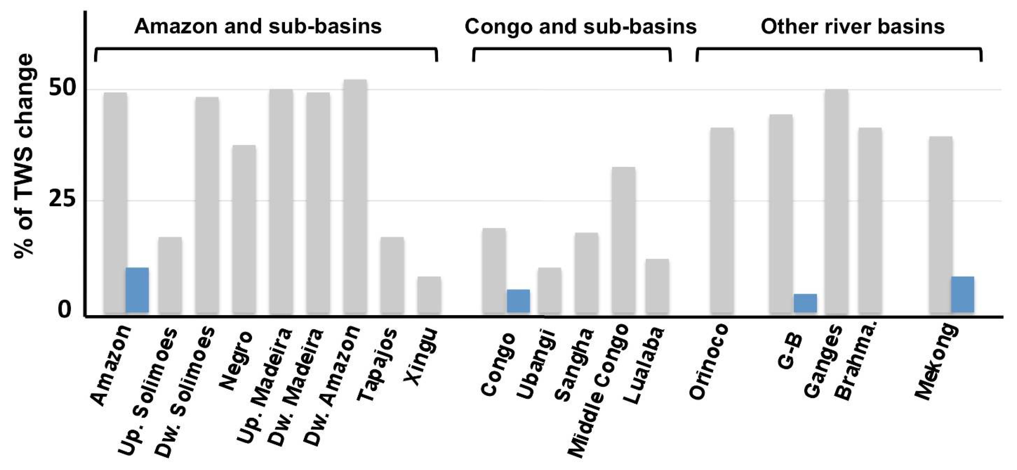
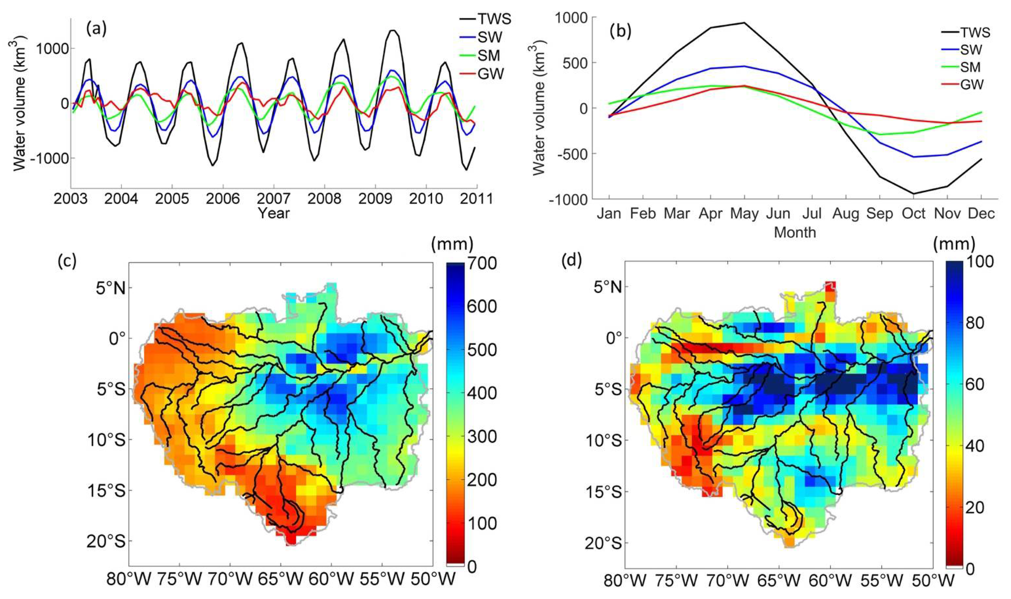
4.3. Relative Contribution of SWS Changes to TWS Variations

SWS changes account for only a portion of the total amount of water that moves through the different water storage reservoirs of a drainage basin (Equation (2)). However, the relative contribution of the spatiotemporal variations of these freshwater reservoirs remains widely unknown at a large scale. Since the launch of GRACE, we have improved our knowledge of the TWS spatiotemporal variations, but studies that isolate the individual contributions of the component storage anomalies from TWS rely mainly on land surface models [39,171]. The authors of [39] suggested that SWS contributes 8% of TWS variability globally, but with large differences among climate zones, with SWS being a principal driver of TWS variability in the tropics (41% in the Amazon), confirming the key role of SWS component of TWS variability. Across China, contributions of surface water changes to the trend of terrestrial water storage anomalies were provided in [172], also using model outputs and GRACE TWS. However, these estimates can differ substantially between studies, especially in humid environments and in monsoon-dominated river basins, for which the disagreement can be large, with results that quantify the contributions of SWS to TWS sometimes varying from 5% up to more than 50% over the same region.

Satellite-based observations of SWS changes allow a novel estimate of their relative contributions to TWS variations. The surface water volume changes averaged over the Rio Negro basin were firstly compared to GRACE-based TWS changes, in an annual cycle [127] and over two concurrent years [129], confirming the hypothesis for this basin that TWS changes are almost equally partitioned (~50%) between surface water and the combination of soil moisture and groundwater.

At the scale of the Amazon basin, about half (45% in [70,130] and 50% in [78]) of the variations in the total amount of water as detected using GRACE data occur in the river system, wetlands, and floodplains as surface water storage. This figure reached 61% in [134]. These results are on the same order of magnitude as previous accepted results on the partition of TWS into contributing hydrological storages in the Amazon [173], based on model simulations; combining a land surface model and a global runoff routing scheme, Ref. [77] suggested that river storage explains ~73% of TWS variation, while [76], based on simulations from Global Land Data Assimilation System (GLDAS) Noah Land Surface Model, and [174], using the Interactions between Soil–Biosphere–Atmosphere (ISBA) land surface model, both indicated that TWS variations in the Amazon are almost equally partitioned into soil moisture and river storage variations. Modeling results from WGHM [175] suggested that surface water storage contributes to ~40% of seasonal TWS variations in the Amazon, while, using the MGB-IPH model, Ref. [157] estimated that surface waters dominate TWS for the whole Amazon area with a fraction of 56%. However, Ref. [171], which provided relative contributions of SWS to TWS for 168 basins globally using individual components of TWS averaged from six land surface models and GRACE, reported lower values (Figure 6).

The contribution of SWS to TWS variability also varies greatly geographically within a basin, with different relative contributions among each sub-basin (Figure 6). Over the Amazon, this contribution varies from more than 50% downstream the basin to only a few percent in the Xingu sub-basin. The same conclusions were made over the Congo River Basin, where the contribution of SWS to TWS variability is very heterogeneous among the sub-basins [132]. For the entire Congo River Basin, the seasonal SWS variations represent 19% ± 5% of the TWS variations, while they account for 10% ± 1% in the Ubangi basin and 18% ± 1% in the Sangha, 33% ± 7% in the Middle Congo, encompassing extensive floodplains and wetlands, and 12% ± 2% in the Lwalaba sub-basins. Over the Central Congo, these numbers are in good agreement with those provided by [114] over smaller regions with floodplains and wetlands. For other river basins, mainly located in the tropical band, estimates of SWS changes to TWS variability range from 40% for the Lower Mekong [139] to 45% in the Orinoco [131] and the Ganges–Brahmaputra [132], with a difference between the Ganges (∼51%) and the Brahmaputra (∼41%) basins [159]. One can notice some differences between the two major tropical basins of Amazon and Congo. While, in the Amazon, SWS contribution to TWS variations is generally around 50%, it is below 20% for the Congo, except in the Middle Congo region, which is characterized by extensive floodplains. This needs further investigations to better understand the main drivers of these differences [68,131]. Similarly, the Ganges–Brahmaputra and Mekong River basins, which host extensive floodplains, especially in their delta region, also show higher contributions of SWS to TWS variability. For river basins over northern regions, no such estimates exist, despite the importance of SWS variations to TWS changes [176]. Figure 6 also compares the relative contributions of SWS to TWS variations obtained from remote sensing and from an ensemble of global land surface models [171] over the Amazon, the Congo, the Ganges–Brahmaputra and the Mekong. In general, global land surface model output estimates give lower contributions of SWS to TWS as estimated from remote sensing or from regional models. Over these four basins, the contributions of SWS to TWS variations from the global land surface models was found between 5% and 10%, a factor of 5–6 lower than the satellite-based estimates. This calls for more investigations and comparisons of the various estimates and supports the need for a better representation of surface water dynamics in global-scale models [39,41,176].

4.4. Toward Subsurface and Groundwater Variation Estimates Using Satellite-Derived SWS in Combination with GRACE TWS

While surface water remains the principal freshwater supply that meets human water demand globally and is the source of most of the water used by humans, our dependence on groundwater has increased over time. Groundwater is now the primary source of freshwater for approximately two billion people, while half or more of the irrigation water used to grow the world’s food is supplied from underground sources [23,177]. Subsurface reservoirs are now being disrupted by human activities such as pumping of fossil water to the surface for irrigation and human water resources. However, our knowledge on the state of large groundwater systems is very limited [71,178], largely because of the prohibitive cost and complexity of monitoring large aquifer systems. Several studies reported that, in some regions, such as the Indian subcontinent, as current groundwater withdrawal possibly exceeds the potential groundwater recharge, a reduction in long-term groundwater storage, referred to as “groundwater depletion”, is evidenced. In northern India and Bangladesh [73], the intensive use and over-abstraction of groundwater for dry-season irrigation and city water supply has led to a rapid decline in groundwater tables in many parts of the country [74]. Accurate partitioning of GRACE-derived TWS into the different water storage contributions is, therefore, critical in quantifying subsurface and GWS changes (Equation (2)). Several studies have estimated GWS changes from GRACE-derived TWS change after deducting the contribution of changes in the other water storage compartments. Auxiliary information on the other components of TWS, from either in situ observations or land-surface models, was used to produce a timeseries of groundwater storage anomalies [179].

The quantification of SWS changes from satellites enables the proposal of another approach to estimate “subsurface water storages” (the sum of GWS and SMS changes) and/or GWS changes from GRACE data. Disaggregation of GRACE-derived TWS into satellite-derived subsurface water storage variations was carried out using SWS estimates from satellites. In many studies, the choice of estimating the sole subsurface water storage variations instead of disaggregating this term into GWS and SMS changes was driven by the poor quality, and the large uncertainties associated with existing products of soil moisture at a large scale from satellite-derived (AMSR-E, SMOS, and SMAP) are representative of the very first cm below the surface [180]. Moreover, it is assumed that the variations in water storage from the canopy are generally negligible and, hence, not considered.

Timeseries of subsurface water changes were derived over the Ganges and Brahmaputra rivers basins, with annual amplitudes of ∼290 km³ and 320 km³, respectively [132], in agreement with estimates of the total replenishable groundwater resources in the Ganges River of ∼180 km³/year. However, the timeseries over 2003–2007 were too short to study the “groundwater depletion” in the region. Nevertheless, anomalies of subsurface water storage were mapped during the 2006 large drought that affected the northern part of India, with clear patterns of deficit of subsurface water in the southern tributaries of the Ganges River. Timeseries of subsurface changes were also obtained over the Congo and its sub-basins [133] and the lower Mekong [139].

Over the Amazon, an ensemble of information on soil moisture changes at basin-scale from models were used to further disaggregate subsurface anomalies and to derive GWS changes [70,127]. Figure 7 shows the first available timeseries and maps of GWS changes over the Amazon. These GWS estimates are in good agreement locally with in situ groundwater observations [70,127], and the basin-scale results agree well with spatial patterns of hydrogeological maps of the region (e.g., GW recharge, porosity maps, and aquifer boundaries). The seasonal amplitude of GWS contributes 20–35% of the GRACE-derived TWS amplitude, and the impact of the 2005 drought was also observed in the form of a GWS anomaly and lasted several years [70].

Similarly, a combination of satellite-derived SWS and the root zone soil moisture obtained from the Global Land Evaporation Amsterdam Model (GLEAM) was also used to show that, over the Lake Chad region, TWS changes and trends are strongly controlled by groundwater variations, which plays an important role in controlling the water cycle over the entire Lake Chad basin [141]. Such studies call for a better understanding of water storage changes and aquifer properties, such as soil characteristics [181], recharge and permeability properties [182], and how groundwater responds to the influence of climatic factors, vegetation behavior, and basin characteristics.

5. The Future with the Surface Water and Ocean Topography Mission: New Opportunities for Hydrological and Multidisciplinary Sciences

Despite the growing effort to better quantify SWS changes at various spatiotemporal scales using remote sensing observations, the previous sections highlighted that surface water storage in rivers, floodplains, and wetlands is still currently poorly monitored. Therefore, this leaves open questions for the hydrologic processes, the climate influence, and the human impacts controlling surface water storage and its transport on continents. Most estimates have spatial and temporal resolutions adequate to study large-scale regions, from seasonal to interannual variability timescales, but are not appropriate for finer-scale studies.

If, to date, no past or current satellite mission has yet been specifically designed to observe SWS changes at the global scale, this will soon be one of the goals of the upcoming Surface Water and Ocean Topography (SWOT) satellite mission [81,87]. A collaboration among the United States National Aeronautics and Space Administration (NASA), Centre National d’Études Spatiales (CNES, the French Spatial Agency), the Canadian Space Agency, and the United Kingdom Space Agency, the SWOT launch is now planned for 2022. SWOT can be seen as a “topographic imager” satellite mission with ~100 m spatial resolution based on synthetic aperture radar (SAR) interferometry, which will provide measurements of surface water elevation, slope, and water mask, with a temporal resolution of 21 days in a predefined inland water mask. More details about SAR interferometry and the KaRIn measurements onboard SWOT can be found in [183]. Its capability to measure height and surface changes will help characterize variations in river discharge and lake water storage [12] in all rivers wider than 100 m and water bodies greater than 250 m × 250 m in areas under the swath coverage.

As stated in its mission science requirements document [184], a global water mask following the shorelines of all observed individual water bodies will be provided at least once every repeat cycle, along with its water elevation, enabling the derivation of water storage within each such water body, thus providing the first globally consistent product of river and lake storage variations. Even if it is not one of the mission requirements, SWOT will also provide observations in floodplains and wetland environments, even if the set of observables of such water bodies is still uncertain. In floodplains and wetlands environments, characterized by large extents of open water and sparse vegetation, SWOT will potentially provide observations of water surface elevation and extent, a combination which will measure SWS changes. In regions with denser vegetation, to what extent SWOT observations will be affected by vegetation is still unknown and requires more studies. Nevertheless, SWOT may provide useful information to be exploited even if sampling under dense vegetation remains limited, which will open new ways to investigate and observe those regions and the hydrology of inundated vegetation systems.

As demonstrated in this review, the products and advances made in terms of SWS estimates from remote sensing provide a solid baseline and an unprecedented source of information to evaluate and validate SWOT measurements after its launch, and they represent a valuable benchmark for future hydrological applications.

In this regard, in order to facilitate the development of such opportunities, we believe that it is necessary for the community to have more access to the existing tools that can be used for the purpose of SWS monitoring, as well as existing repositories of useful data. As of today, there are some initiatives such as the Centre d’Expertise Scientifique from the French data center THEIA-LAND (CES), https://www.theia-land.fr/en/ceslist/water-volumes-sec/ last accessed on 13 October 2021), or such as the French Observation Service dedicated to satellite altimetry studies (Centre of Topography of the Oceans and the Hydrosphere) at LEGOS, Toulouse, France (http://ctoh.legos.obs-mip.fr/applications/land_surfaces/hydrologic_products/hauteurs-deau-et-volume last accessed on 13 October 2021), which are trying to gather useful tools and to offer some guidance and data access to SWS products. However, these initiatives and their repositories are still under development, and the effort needs to grow, especially in the context of SWOT. One goal of the present review is to foster such initiatives so that the scientific community, space agencies, and data centers will support the development of such tools and repositories, similarly to what has been done for sea level and water elevation from radar altimetry in the last decades. Such initiatives could be hosted by the Archiving, Validation, and Interpretation of Oceanographic Satellite Data (AVISO+, https://www.aviso.altimetry.fr/en/missions/future-missions/swot.html last accessed on 13 October 2021) or the Physical Oceanography Distributed Active Archive Center (PODAAC) hosted by JPL (https://podaac.jpl.nasa.gov/SWOT last accessed on 13 October 2021).

The present review also highlighted the fact that SWS estimates are currently available only for a few regions worldwide and are mainly limited to large river basins. There is an obvious need to expand investigations to more river basins and regions, covering all climate and environments, including medium-size basins and local-scale studies. One of the opportunities resides in the use of denser VS networks provided by satellite altimetry missions such as S3-A/B in combination with GIEMS [84,85,117], SWAMPS [86], or SWAF [162]. The use of the hypsometric curve approach with DEM should also be investigated in the future with a goal to retrieve SWS variations on the global scale.

Additionally, the benefits of accurate and comprehensive SWS change estimates at large scale are very valuable for many aspects of hydrological science, climate science, and water management. Moreover, future progress and advances, thanks to new methodological developments or directly from SWOT observations, for instance, will also provide new opportunities for synergetic sciences. Here, we summarized a few potential avenues that have been identified.

Hydrological and hydraulic modeling: Hydrological and hydraulic models are evaluated and/or calibrated against independent observations, from in situ measurements or from satellite-derived products. Unlike surface water elevation, surface water extent, or river discharge, which are common variables used to evaluate hydrological simulation outputs [43,157], SWS changes are not yet commonly used to evaluate model performance. However, it remains an important variable to be better constrained within modeling systems. Few recent modeling studies addressed the surface water storage components [39,43,157,172,185] regionally or globally, but more efforts are needed in order to better represent the surface water storage complexity and understand flood dynamics. SWS estimates could also trigger applications based on 2D modeling to better constrain floodplain storage changes and diffuse flow in floodplains and wetlands [185]. The availability of satellite SWS estimates, therefore, opens new opportunities for the improvement and new developments of hydrological and hydraulic modeling.

Data assimilation: Several studies were developed to assimilate water storage into hydrodynamic and hydrology models, but they were mainly limited to GRACE-derived TWS [186,187,188], soil moisture [189], or both [190,191], leaving great opportunity to improve the performance of models through data assimilation of SWS or GWS. For instance, in an environment such as the Ganges Delta, where surface water storage plays a primary role in TWS and GWS variations, Ref. [192] demonstrated the advantages of removing SWS contributions from GRACE TWS data to better constrain soil moisture and groundwater model outputs and assess the significant decline in groundwater storage in Bangladesh. Along with river discharge and water levels, the use of SWS data from the upcoming SWOT in order to correct model parameters will also bring new opportunities [193,194,195,196].

Implications of land–ocean exchanges: Climate-driven or human-driven changes in water stored on land are important components of sea-level budgets [197] and play a role in present global and regional sea-level rise [198,199,200]. The annual cycle of land water storage moved through the seasonal distribution of water from ocean to land is estimated to be 17 ± 4 mm of sea-level equivalent [201], but large uncertainties remain on the individual contributions of SWS or GWS fluctuations and their impacts on global and regional sea-level variability [198,202]. Global SWS estimates will help better quantify the influence of land water storage on the variability and rate of sea-level rise [203,204]. SWS changes are also important information to investigate the dynamics of freshwater in deltaic regions, as water storage, especially in terms of SWS and GWS, which are at play among the various factors controlling the subsidence [205] or saline intrusion [206,207,208] in such regions.

Water management: As part of the global freshwater resources, SWS is important to human life and activities, and proper management is needed for their sustainability. Here, we dealt with SWS in rivers and wetlands, but large amounts of freshwater are stored in ponds, lakes, and reservoirs, which are often now human-managed [60] through dams and other human interventions. Global SWS estimates will help to have a better knowledge of the amount of freshwater that is stored on the Earth’s surface and how it changes over time. Therefore, there is a need for a comprehensive monitoring of SWS over its various components, from SWS in reservoirs/lakes to SWS in rivers and wetlands, and this could be achieved by integrating and merging the various satellite techniques mentioned. In particular, this will be useful to basin-scale water resources management and the relative contribution of the natural and human-induced variability. For this purpose, finer temporal sampling of the estimates, ideally daily, should be achieved thanks to the future capabilities of the next generation of radar altimetry mission aimed at daily revisit, such as the Small Altimetry Satellite for Hydrology (SMASH) constellation.

6. Summary and Perspectives

In this work, we addressed the role of remote sensing in estimating surface water storage changes over continents and how these estimates contribute to improve our knowledge in hydrological sciences of large river basins. We focused on the amount of freshwater stored in rivers/wetlands/floodplains and its variations, a key component of the water cycle, land surface hydrology, and water resources management, for which the impacts of current changes remain uncertain. We reviewed the studies, over the last two decades, that described the advances made using space-borne data to characterize the dynamics of the surface water reservoir and how it helped to better derive the characteristics of other hydrological components, such as subsurface and groundwater storage variations.

Firstly, we reviewed the methodological and technical developments achieved to estimate surface water storage, which highlights that it is still very challenging to measure and obtain accurate estimates for large river basins at adequate time/space sampling. Despite the increasing number of satellite missions, we still currently suffer from a lack of direct measurements of surface freshwater storage and its spatiotemporal variations on a global scale. We, therefore, presented the methodologies and methods that were developed, from InSar techniques to the combination of multisource observations to measure surface water storage for different environments worldwide. In particular, multi-satellite approaches to derive SWS, generally based on the complementarity between satellite-derived observations of the spatiotemporal dynamics of the surface water extent and elevation, are powerful tools, which can provide associated uncertainties, even if they are limited by the current space–time sampling of available observations. Future investigations should combine newly extended (such as GIEMS-2 now available 1992–2015) or new products, such as the current altimetry observations from S3-A/B, which offer a dense network of VS.

Then, we presented how the use of SWS estimates contributes to a better understanding of large-scale hydrological processes and to the continental water cycle of large river basins. Several studies provided estimates of seasonal variations of SWS changes across large river basins, mainly in tropical environments, as well as for northern-latitude river basins. From local scale to basin scale, the Amazon River is by far the region that gained the most attention in using SWS estimates for hydrology, which can be justified by the fact it is the basin with the largest amount of water volume change across the hydrological reservoirs (up to 1200 km³ for the surface water annually), more than the Congo, the Orinoco, and the Ganges–Brahmaputra combined. SWS change estimates were also presented across studies as valuable information to characterize the impact of climatic events, such as extreme droughts, on the surface hydrology of large river basins, such as the 2005 event in the Amazon basin. Additionally, the relative contributions of SWS variations to GRACE/GRACE-FO-based TWS changes provide new opportunities to move toward observation-based estimates of subsurface and groundwater storage variations, particularly relevant in environments with extensive floodplains and wetlands, such as in the tropics.

Despite these recent advances, fostered in the last years by an unprecedented availability of concurrent satellite observations, there is still much to be learned regarding SWS changes and their implications for continental water balance, climate feedback, and water management.

The upcoming launch in 2022 of the SWOT satellite mission, which will provide, for the first time, direct estimates of SWS changes on a global scale, will open a new era of scientific advances for continental hydrology and to understand continental water store variability. One priority should be to strengthen the current methodologies and results of studies performed up to now, especially by extending the timeseries to longer periods, by providing more realistic quantifications of the errors and uncertainties in the multi-satellites approaches. Furthermore, studies that use the complementarity with other satellite observations of the different components of the water cycle, which will be simultaneously available with SWOT, should be encouraged and supported to improve the monitoring of the water cycle as a whole. This future progress and these advances will foster new opportunities for synergetic sciences, in hydrological modeling, data assimilation, land–ocean interactions, and water management.

Lastly, in the current development of the concept of essential variables (EVs) in the scientific communities, which are chosen and defined to represent a set of variables that help describe and monitor the evolution of Earth system components [209,210], we believe that this work and the forthcoming progress will contribute to the call by hydrological and remote sensing communities for surface water storage, in complement to water level and extent, to be considered in the coming years as an essential water variable [211].

References

1. Vörösmarty, C.J.; Green, P.; Salisbury, J.; Lammers, R.B. Global Water Resources: Vulnerability from Climate Change and Population Growth. Science 2000, 289, 284–288. [Google Scholar] [CrossRef] [Green Version]
2. Vörösmarty, C.J.; McIntyre, P.B.; Gessner, M.O.; Dudgeon, D.; Prusevich, A.; Green, P.; Glidden, S.; Bunn, S.E.; Sullivan, C.A.; Liermann, C.R.; et al. Global threats to human water security and river biodiversity. Nature 2010, 467, 555–561. [Google Scholar] [CrossRef]
3. Steffen, W.; Richardson, K.; Rockström, J.; Cornell, S.E.; Fetzer, I.; Bennett, E.M.; Biggs, R.; De Carpenter, S.R.; Carpenter, S.R.; De Vries, W.; et al. Planetary boundaries: Guiding human development on a changing planet. Science 2015, 347, 1259855. [Google Scholar] [CrossRef] [PubMed] [Green Version]
4. Seddon, A.; Macias-Fauria, M.; Long, P.R.; Benz, D.; Willis, K. Sensitivity of global terrestrial ecosystems to climate variability. Nature 2016, 531, 229–232. [Google Scholar] [CrossRef] [PubMed] [Green Version]
5. Albert, J.S.; Destouni, G.; Duke-Sylvester, S.M.; Magurran, A.E.; Oberdorff, T.; Reis, R.E.; Winemiller, K.O.; Ripple, W.J. Scientists’ warning to humanity on the freshwater biodiversity crisis. Ambio 2021, 50, 85–94. [Google Scholar] [CrossRef] [PubMed]
6. Chahine, M.T. The hydrological cycle and its influence on climate. Nature 1992, 359, 373–380. [Google Scholar] [CrossRef]
7. Shiklomanov, I.A.; Rodda, J.C. World Water Resources at the Beginning of the Twenty-First Century; Cambridge University Press: Cambridge, UK, 2003. [Google Scholar]
8. Stephens, G.L.; Slingo, J.M.; Rignot, E.; Reager, J.T.; Hakuba, M.Z.; Durack, P.J.; Worden, J.; Rocca, R. Earth’s water reservoirs in a changing climate. Proc. R. Soc. A 2020, 476, 20190458. [Google Scholar] [CrossRef] [PubMed] [Green Version]
9. Boberg, J. Freshwater Availability. In Liquid Assets: How Demographic Changes and Water Management Policies Affect Freshwater Resources; RAND Corporation: Santa Monica, CA, USA; Arlington, VA, USA; Pittsburgh, PA, USA, 2005; pp. 15–28. Available online: http://www.jstor.org/stable/10.7249/mg358cf.9 (accessed on 13 October 2021).
10. Zhou, T.; Nijssen, B.; Gao, H.; Lettenmaier, D.P. The Contribution of Reservoirs to Global Land Surface Water Storage Variations. J. Hydrometeorol. 2016, 17, 309–325. [Google Scholar] [CrossRef]
11. Alsdorf, D.E.; Rodríguez, E.; Lettenmaier, D.P. Measuring surface water from space. Rev. Geophys. 2007, 45, RG2002. [Google Scholar] [CrossRef]
12. Good, S.P.; Noone, D.; Bowen, G. Hydrologic connectivity constrains partitioning of global terrestrial water fluxes. Science 2015, 349, 175–177. [Google Scholar] [CrossRef] [Green Version]
13. Trenberth, K.E.; Smith, L.; Qian, T.; Dai, A.; Fasullo, J. Estimates of the global water budget and its annual cycle using observational and model data. J. Hydrometeorol. 2007, 8, 758–769. [Google Scholar] [CrossRef]
14. Trenberth, K.E.; Fasullo, J.; Mackaro, J. Atmospheric Moisture Transports from Ocean to Land and Global Energy Flows in Reanalyses. J. Clim. 2011, 24, 4907–4924. [Google Scholar] [CrossRef]
15. Oki, T.; Kanae, S. Global Hydrological Cycles and World Water Resources. Science 2006, 313, 1068–1072. [Google Scholar] [CrossRef] [Green Version]
16. Hall, J.W.; Grey, D.; Garrick, D.; Fung, F.; Brown, C.; Dadson, S.J.; Sadoff, C.W. Coping with the curse of freshwater variability: Institutions, infrastructure, and information for adaptation. Science 2014, 346, 429–430. [Google Scholar] [CrossRef]
17. Rodell, M.; Famiglietti, J.S.; Wiese, D.N.; Reager, J.T.; Beaudoing, H.K.; Landerer, F.W.; Lo, M.-H. Emerging trends in global freshwater availability. Nature 2018, 557, 651–659. [Google Scholar] [CrossRef] [PubMed]
18. Lorenz, C.; Kunstmann, H. The Hydrological Cycle in Three State-of-the-Art Reanalyses: Intercomparison and Performance Analysis. J. Hydrometeorol. 2012, 13, 1397–1420. [Google Scholar] [CrossRef] [Green Version]
19. Trenberth, K.E.; Asrar, G.R. Challenges and Opportunities in Water Cycle Research: WCRP Contributions. Surv. Geophys. 2014, 35, 515–532. [Google Scholar] [CrossRef]
20. Milly, P.C.D.; Dunne, K.A.; Vecchia, A.V. Global pattern of trends in streamflow and water availability in a changing climate. Nature 2005, 438, 347–350. [Google Scholar] [CrossRef] [PubMed]
21. Alcamo, J.; Flörkeand, M.; Märker, M. Future long-term changes in global water resources driven by socio-economic and climatic changes. Hydrolog. Sci. J. 2007, 52, 247–275. [Google Scholar] [CrossRef]
22. Hoekstra, A.Y.; Mekonnen, M.; Chapagain, A.K.; Mathews, R.E.; Richter, B.D. Global Monthly Water Scarcity: Blue Water Footprints versus Blue Water Availability. PLoS ONE 2012, 7, e32688. [Google Scholar] [CrossRef]
23. Famiglietti, J.S. The global groundwater crisis. Nat. Clim. Change 2014, 4, 945–948. [Google Scholar] [CrossRef]
24. Konapala, G.; Mishra, A.K.; Wada, Y.; Mann, M.E. Climate change will affect global water availability through compounding changes in seasonal precipitation and evaporation. Nat. Commun. 2020, 11, 1–10. [Google Scholar] [CrossRef] [PubMed]
25. Maja, M.M.; Ayano, S.F. The Impact of Population Growth on Natural Resources and Farmers’ Capacity to Adapt to Climate Change in Low-Income Countries. Earth Syst. Environ. 2021, 5, 1–13. [Google Scholar] [CrossRef]
26. Valipour, M.; Bateni, S.; Jun, C. Global Surface Temperature: A New Insight. Climate 2021, 9, 81. [Google Scholar] [CrossRef]
27. Gain, A.K.; Wada, Y. Assessment of Future Water Scarcity at Different Spatial and Temporal Scales of the Brahmaputra River Basin. Water Resour. Manag. 2014, 28, 999–1012. [Google Scholar] [CrossRef]
28. Haddeland, I.; Heinke, J.; Biemans, H.; Eisner, S.; Flörke, M.; Hanasaki, N.; Konzmann, M.; Ludwig, F.; Masaki, Y.; Schewe, J.; et al. Water, human impacts, and climate change. Proc. Natl. Acad. Sci. USA 2014, 111, 3251–3256. [Google Scholar] [CrossRef] [Green Version]
29. Mehran, A.; AghaKouchak, A.; Nakhjiri, N.; Stewardson, M.J.; Peel, M.C.; Phillips, T.J.; Wada, Y.; Ravalico, J.K. Compounding Impacts of Human-Induced Water Stress and Climate Change on Water Availability. Sci. Rep. 2017, 7, 6282. [Google Scholar] [CrossRef] [Green Version]
30. Chawla, I.; Karthikeyan, L.; Mishra, A.K. A review of remote sensing applications for water security: Quantity, quality, and extremes. J. Hydrol. 2020, 585, 124826. [Google Scholar] [CrossRef]
31. Alsdorf, D.E.; Lettenmaier, D.P. Tracking fresh water from space. Science 2003, 301, 1492–1494. [Google Scholar] [CrossRef] [Green Version]
32. Rodell, M.; Beaudoing, H.K.; L’Ecuyer, T.S.; Olson, W.S.; Famiglietti, J.; Houser, P.R.; Adler, R.; Bosilovich, M.G.; Clayson, C.A.; Chambers, D.; et al. The Observed State of the Water Cycle in the Early Twenty-First Century. J. Clim. 2015, 28, 8289–8318. [Google Scholar] [CrossRef]
33. O’Connell, E. Towards Adaptation of Water Resource Systems to Climatic and Socio-Economic Change. Water Resour. Manag. 2017, 31, 2965–2984. [Google Scholar] [CrossRef]
34. Peixoto, J.P.; Oort, A.H. Oort Physics of Climate; American Institute of Physics Press: Woodbury, NY, USA, 1992. [Google Scholar]
35. Lettenmaier, D.P. Observations of the global water cycle—Global monitoring networks. In Encyclopedia of Hydrologic Sciences; Anderson, M.G., McDonnell, J.J., Eds.; John Wiley: Hoboken, NJ, USA, 2005; Volume 5, pp. 2719–2732. [Google Scholar]
36. Sheffield, J.; Ferguson, C.R.; Troy, T.; Wood, E.; McCabe, M. Closing the terrestrial water budget from satellite remote sensing. Geophys. Res. Lett. 2009, 36, L07403. [Google Scholar] [CrossRef]
37. Dorigo, W.; Dietrich, S.; Aires, F.; Brocca, L.; Carter, S.; Cretaux, J.; Dunkerley, D.; Enomoto, H.; Forsberg, R.; Güntner, A.; et al. Closing the water cycle from observations across scales:Where do we stand? Bull. Am. Meteorol. Soc. 2021, 102, 10. Available online: https://journals.ametsoc.org/view/journals/bams/aop/BAMS-D-19-0316.1/BAMS-D-19-0316.1.xml (accessed on 13 October 2021). [CrossRef]
38. Kinter, J.; Shukla, J. The global hydrologic and energy cycles: Suggestions for studies in the pre-Global Energy and Water Cycle Experiment (GEWEX) period. Bull. Amer. Meteor. Soc. 1990, 71, 181–189. [Google Scholar] [CrossRef] [Green Version]
39. Getirana, A.; Kumar, S.; Girotto, M.; Rodell, M. Rivers and Floodplains as Key Components of Global Terrestrial Water Storage Variability. Geophys. Res. Lett. 2017, 44, 10359–10368. [Google Scholar] [CrossRef] [Green Version]
40. Papa, F.; Durand, F.; Rossow, W.B.; Rahman, A.; Bala, S.K. Seasonal and Interannual Variations of the Ganges-Brahmaputra River Discharge, 1993-2008 from satellite altimeters. J. Geophys. Res. 2010, 115, C12013. [Google Scholar] [CrossRef] [Green Version]
41. Yamazaki, D.; Kanae, S.; Kim, H.; Oki, T. A physically based description of floodplain inundation dynamics in a global river routing model. Water Resour. Res. 2011, 47, W04501. [Google Scholar] [CrossRef]
42. Döll, P.; Douville, H.; Güntner, A.; Schmied, H.M.; Wada, Y. Modelling Freshwater Resources at the Global Scale: Challenges and Prospects. Surv. Geophys. 2016, 37, 195–221. [Google Scholar] [CrossRef] [Green Version]
43. Siqueira, V.A.; Paiva, R.C.D.; Fleischmann, A.S.; Fan, F.M.; Ruhoff, A.L.; Pontes, P.R.M.; Paris, A.; Calmant, S.; Collischonn, W. Toward continental hydrologic–hydrodynamic modeling in South America. Hydrol. Earth Syst. Sci. 2018, 22, 4815–4842. [Google Scholar] [CrossRef] [Green Version]
44. Decharme, B.; Delire, C.; Minvielle, M.; Colin, J.; Vergnes, J.-P.; Alias, A.; Saint-Martin, D.; Séférian, R.; Sénési, S.; Voldoire, A. Recent Changes in the ISBA-CTRIP Land Surface System for Use in the CNRM-CM6 Climate Model and in Global Off-Line Hydrological Applications. J. Adv. Model. Earth Syst. 2019, 11, 1207–1252. [Google Scholar] [CrossRef]
45. Müller Schmied, H.; Cáceres, D.; Eisner, S.; Flörke, M.; Herbert, C.; Niemann, C.; Peiris, T.A.; Popat, E.; Portmann, F.T.; Reinecke, R.; et al. The global water resources and use model WaterGAP v2.2d: Model description and evaluation. Geosci. Model Dev. 2021, 14, 1037–1079. [Google Scholar] [CrossRef]
46. Sood, A.; Smakhtin, V. Global hydrological models: A review. Hydrol. Sci. J. 2015, 60, 549–565. [Google Scholar] [CrossRef]
47. Scanlon, B.R.; Zhang, Z.; Rateb, A.; Sun, A.; Wiese, D.; Save, H.; Beaudoing, H.; Lo, M.H.; Müller-Schmied, H.; Döll, P.; et al. Tracking Seasonal Fluctuations in Land Water Storage Using Global Models and GRACE Satellites. Geophys. Res. Lett. 2019, 46, 5254–5264. [Google Scholar] [CrossRef]
48. Cazenave, A.; Milly, P.C.D.; Douville, H.; Benveniste, J.; Kosuth, P.; Lettenmaier, D.P. Space techniques used to measure change in terrestrial waters. Eos Trans. AGU 2004, 85, 59. [Google Scholar]
49. Famiglietti, J.S.; Cazenave, A.; Eicker, A.; Reager, J.T.; Rodell, M.; Velicogna, I. Satellites provide the big picture. Science 2015, 349, 684–685. [Google Scholar] [CrossRef] [Green Version]
50. Tapley, B.D.; Bettadpur, S.; Ries, J.C.; Thompson, P.F.; Watkins, M.M. GRACE Measurements of Mass Variability in the Earth System. Science 2004, 305, 503–505. [Google Scholar] [CrossRef] [Green Version]
51. Scanlon, B.R.; Zhang, Z.; Save, H.; Sun, A.; Schmied, H.M.; van Beek, L.P.H.; Wiese, D.N.; Wada, Y.; Long, D.; Reedy, R.C.; et al. Global models underestimate large decadal declining and rising water storage trends relative to GRACE satellite data. Proc. Natl. Acad. Sci. USA 2018, 115, E1080–E1089. [Google Scholar] [CrossRef] [Green Version]
52. Pokhrel, Y.; Felfelani, F.; Satoh, Y.; Boulange, J.; Burek, P.; Gädeke, A.; Gerten, D.; Gosling, S.N.; Grillakis, M.; Gudmundsson, L.; et al. Global terrestrial water storage and drought severity under climate change. Nat. Clim. Chang. 2021, 11, 226–233. [Google Scholar] [CrossRef]
53. Vishwakarma, B.D.; Bates, P.; Sneeuw, N.; Westaway, R.M.; Bamber, J.L. Re-assessing global water storage trends from GRACE time series. Environ. Res. Lett. 2021, 16, 034005. [Google Scholar] [CrossRef]
54. Rodell, M.; Famiglietti, J. The potential for satellite-based monitoring of groundwater storage changes using GRACE: The High Plains aquifer, Central US. J. Hydrol. 2002, 263, 245–256. [Google Scholar] [CrossRef] [Green Version]
55. Duncan, B.N.; Ott, L.E.; Abshire, J.B.; Brucker, L.; Carroll, M.L.; Carton, J.; Comiso, J.C.; Dinnat, E.P.; Forbes, B.C.; Gonsamo, A.; et al. Space-Based Observations for Understanding Changes in the Arctic-Boreal Zone. Rev. Geophys. 2020, 58, e2019RG000652. [Google Scholar] [CrossRef]
56. Chang, A.; Foster, J.; Hall, D. Nimbus-7 SMMR Derived Global Snow Cover Parameters. Ann. Glaciol. 1987, 9, 39–44. [Google Scholar] [CrossRef] [Green Version]
57. Kerr, Y.; Waldteufel, P.; Wigneron, J.-P.; Martinuzzi, J.; Font, J.; Berger, M. Soil moisture retrieval from space: The Soil Moisture and Ocean Salinity (SMOS) mission. IEEE Trans. Geosci. Remote. Sens. 2001, 39, 1729–1735. [Google Scholar] [CrossRef]
58. Entekhabi, D.; Njoku, E.G.; O’Neill, P.E.; Kellogg, K.H.; Crow, W.T.; Edelstein, W.N.; Entin, J.K.; Goodman, S.D.; Jackson, T.J.; Johnson, J.; et al. The Soil Moisture Active Passive (SMAP) Mission. Proc. IEEE 2010, 98, 704–716. [Google Scholar] [CrossRef]
59. Mekonnen, M.M.; Hoekstra, A.Y. Sustainability: Four billion people facing severe water scarcity. Sci. Adv. 2016, 2, e1500323. [Google Scholar] [CrossRef] [Green Version]
60. Cooley, S.W.; Ryan, J.C.; Smith, L.C. Human alteration of global surface water storage variability. Nature 2021, 591, 78–81. [Google Scholar] [CrossRef]
61. Richey, J.E.; Melack, J.M.; Aufdenkampe, A.; Ballester, V.M.; Hess, L.L. Outgassing from Amazonian rivers and wetlands as a large tropical source of atmospheric CO2. Nature 2002, 416, 617–620. [Google Scholar] [CrossRef] [PubMed]
62. Raymond, P.A.; Hartmann, J.; Lauerwald, R.; Sobek, S.; McDonald, C.; Hoover, M.; Butman, D.; Striegl, R.; Mayorga, E.; Humborg, C.; et al. Global carbon dioxide emissions from inland waters. Nature 2013, 503, 355–359. [Google Scholar] [CrossRef] [PubMed] [Green Version]
63. Melack, J.M.; Forsberg, B.R. Biogeochemistry of Amazon floodplain lakes and associated wetlands. In The Bio-Geochemistry of the Amazon Basin; McClain, M.E., Victoria, R.L., Richey, J.E., Eds.; Oxford University Press: New York, NY, USA, 2001; pp. 235–274. [Google Scholar]
64. Ward, N.D.; Bianchi, T.; Medeiros, P.M.; Seidel, M.; Richey, J.E.; Keil, R.G.; Sawakuchi, H.O. Where Carbon Goes When Water Flows: Carbon Cycling across the Aquatic Continuum. Front. Mar. Sci. 2017, 4. [Google Scholar] [CrossRef] [Green Version]
65. Krinner, G. Impact of lakes and wetlands on boreal climate. J. Geophys. Res. 2003, 108, 4520. [Google Scholar] [CrossRef]
66. Decharme, B.; Douville, H.; Prigent, C.; Papa, F.; Aires, F. A new river flooding scheme for global climate applications: Off-line evaluation over South America. J. Geophys. Res. 2008, 113, D11110. [Google Scholar] [CrossRef]
67. Reis, V.; Hermoso, V.; Hamilton, S.K.; Ward, D.; Fluet-Chouinard, E.; Lehner, B.; Linke, S. A Global Assessment of Inland Wetland Conservation Status. Bioscience 2017, 67, 523–533. [Google Scholar] [CrossRef]
68. Wohl, E. An Integrative Conceptualization of Floodplain Storage. Rev. Geophys. 2021, 59, e2020RG000724. [Google Scholar] [CrossRef]
69. Eriyagama, N.; Smakhtin, V.; Udamulla, L. How much artificial surface storage is acceptable in a river basin and where should it be located: A review. Earth-Science Rev. 2020, 208, 103294. [Google Scholar] [CrossRef]
70. Frappart, F.; Papa, F.; Güntner, A.; Tomasella, J.; Pfeffer, J.; Ramillien, G.; Emilio, T.; Schietti, J.; Seoane, L.; da Silva Carvalho, J.; et al. The spatio-temporal variability of groundwater storage in the Amazon River Basin. Adv. Water Resour. 2019, 124, 41–52. [Google Scholar] [CrossRef] [Green Version]
71. Chen, J.; Famiglietti, J.S.; Scanlon, B.R.; Rodell, M. Groundwater storage changes: Present status from GRACE observations. Surv. Geophys. 2016, 37, 397–417. [Google Scholar] [CrossRef]
72. Shamsudduha, M.; Taylor, R.G. Groundwater storage dynamics in the world’s large aquifer systems from GRACE: Uncertainty and role of extreme precipitation. Earth Syst. Dyn. 2020, 11, 755–774. [Google Scholar] [CrossRef]
73. Rodell, M.; Velicogna, I.; Famiglietti, J.S. Satellite-based estimates of groundwater depletion in India. Nature 2009, 460, 999–1002. [Google Scholar] [CrossRef] [Green Version]
74. Tiwari, V.M.; Wahr, J.; Swenson, S. Dwindling groundwater resources in northern India, from satellite gravity observations. Geophys. Res. Lett. 2009, 36, L18401. [Google Scholar] [CrossRef] [Green Version]
75. Shamsudduha, M.; Taylor, R.; Longuevergne, L. Monitoring groundwater storage changes in the highly seasonal humid tropics: Validation of GRACE measurements in the Bengal Basin. Water Resour. Res. 2012, 48, W02508. [Google Scholar] [CrossRef] [Green Version]
76. Han, S.-C.; Kim, H.; Yeo, I.-Y.; Yeh, P.J.-F.; Oki, T.; Seo, K.-W.; Alsdorf, D.; Luthcke, S.B. Dynamics of surface water storage in the Amazon inferred from measurements of inter-satellite distance change. Geophys. Res. Lett. 2009, 36, L09403. [Google Scholar] [CrossRef] [Green Version]
77. Kim, H.; Yeh, P.J.-F.; Oki, T.; Kanae, S. Role of rivers in the seasonal variations of terrestrial water storage over global basins. Geophys. Res. Lett. 2009, 36, L17402. [Google Scholar] [CrossRef] [Green Version]
78. Papa, F.; Frappart, F.; Güntner, A.; Prigent, C.; Aires, F.; Getirana, A.C.V.; Maurer, R. Surface freshwater storage and variability in the Amazon basin from multi-satellite observations, 1993–2007. J. Geophys. Res. Atmos. 2013, 118, 11951–11965. [Google Scholar] [CrossRef] [Green Version]
79. Cretaux, J.F.; Nielsen, K.; Frappart, F.; Papa, F.; Calmant, S.; Benveniste, J. Hydrological Applications of Satellite Altimetry Rivers, Lakes, Man-Made Reservoirs, Inundated Areas. In Cazenave and Stammer, Satellite Altimetry over Oceans and Land Surfaces; Taylor & Francis Group: New York, NY, USA, 2017; pp. 459–504. [Google Scholar]
80. Mohammadimanesh, F.; Salehi, B.; Mahdianpari, M.; Brisco, B.; Motagh, M. Wetland Water Level Monitoring Using Interferometric Synthetic Aperture Radar (InSAR): A Review. Can. J. Remote Sens. 2018, 44, 247–262. [Google Scholar] [CrossRef]
81. Prigent, C.; Lettenmaier, D.P.; Aires, F.; Papa, F. Towards a High-Resolution Monitoring of Continental Surface Water Extent and Dynamics, at Global Scale: From GIEMS (Global Inundation Extent from Multi-Satellites) to SWOT (Surface Water Ocean Topography). Surv. Geophys. 2016, 37, 339–355. [Google Scholar] [CrossRef] [Green Version]
82. Huang, C.; Chen, Y.; Zhang, S.; Wu, J. Detecting, Extracting, and Monitoring Surface Water from Space Using Optical Sensors: A Review. Rev. Geophys. 2018, 56, 333–360. [Google Scholar] [CrossRef]
83. Pekel, J.-F.; Cottam, A.; Gorelick, N.; Belward, A.S. High-resolution mapping of global surface water and its long-term changes. Nature 2016, 540, 418–422. [Google Scholar] [CrossRef] [PubMed]
84. Prigent, C.; Papa, F.; Aires, F.; Rossow, W.B.; Matthews, E. Global inundation dynamics inferred from multiple satellite observations, 1993–2000. J. Geophys. Res. 2007, 112. [Google Scholar] [CrossRef]
85. Papa, F.; Prigent, C.; Aires, F.; Jimenez, C.; Rossow, W.B.; Matthews, E. Interannual variability of surface water extent at the global scale, 1993–2004. J. Geophys. Res. 2010, 115, 1–17. [Google Scholar] [CrossRef]
86. Schroeder, R.; McDonald, K.C.; Chapman, B.D.; Jensen, K.; Podest, E.; Tessler, Z.D.; Bohn, T.J.; Zimmermann, R. Development and Evaluation of a Multi-Year Fractional Surface Water Data Set Derived from Active/Passive Microwave Remote Sensing Data. Remote. Sens. 2015, 7, 16688–16732. [Google Scholar] [CrossRef] [Green Version]
87. Biancamaria, S.; Lettenmaier, D.P.; Pavelsky, T.M. The SWOT Mission and Its Capabilities for Land Hydrology. Surv. Geophys. 2016, 37, 307–337. [Google Scholar] [CrossRef] [Green Version]
88. Gao, H. Satellite remote sensing of large lakes and reservoirs: From elevation and area to storage. Wiley Interdiscip. Rev. Water 2015, 2, 147–157. [Google Scholar] [CrossRef]
89. Crétaux, J.-F.; Abarca-Del-Río, R.; Bergé-Nguyen, M.; Arsen, A.; Drolon, V.; Clos, G.; Maisongrande, P. Lake Volume Monitoring from Space. Surv. Geophys. 2016, 37, 269–305. [Google Scholar] [CrossRef] [Green Version]
90. Busker, T.; de Roo, A.; Gelati, E.; Schwatke, C.; Adamovic, M.; Bisselink, B.; Pekel, J.-F.; Cottam, A. A global lake and reservoir volume analysis using a surface water dataset and satellite altimetry. Hydrol. Earth Syst. Sci. 2019, 23, 669–690. [Google Scholar] [CrossRef] [Green Version]
91. Tortini, R.; Noujdina, N.; Yeo, S.; Ricko, M.; Birkett, C.M.; Khandelwal, A.; Kumar, V.; Marlier, M.E.; Lettenmaier, D.P. Satellite-based remote sensing data set of global surface water storage change from 1992 to 2018. Earth Syst. Sci. Data 2020, 12, 1141–1151. [Google Scholar] [CrossRef]
92. Bamler, R.; Hartl, P. Synthetic aperture radar interferometry. Inverse Probl. 1998, 14, R1–R54. [Google Scholar] [CrossRef]
93. Alsdorf, D.; Smith, L.; Melack, J. Amazon floodplain water level changes measured with interferometric SIR-C radar. IEEE Trans. Geosci. Remote. Sens. 2001, 39, 423–431. [Google Scholar] [CrossRef]
94. Ramsey, I.E.; Lu, Z.; Rangoonwala, A.; Rykhus, R. Multiple Baseline Radar Interferometry Applied to Coastal Land Cover Classification and Change Analyses. GIScience Remote. Sens. 2006, 43, 283–309. [Google Scholar] [CrossRef] [Green Version]
95. Hanssen, R.F. Radar Interferometry: Data Interpretation and Error Analysis; Springer Science & Business Media: Dordrecht, The Netherlands, 2001; Volume 2. [Google Scholar]
96. Wdowinski, S.; Kim, S.-W.; Amelung, F.; Dixon, T.H.; Miralles-Wilhelm, F.; Sonenshein, R. Space-based detection of wetlands’ surface water level changes from L-band SAR interferometry. Remote. Sens. Environ. 2008, 112, 681–696. [Google Scholar] [CrossRef]
97. Gallant, A.L. The Challenges of Remote Monitoring of Wetlands. Remote. Sens. 2015, 7, 10938–10950. [Google Scholar] [CrossRef] [Green Version]
98. Lu, Z.; Kwoun, O.-I. Radarsat-1 and ERS InSAR Analysis Over Southeastern Coastal Louisiana: Implications for Mapping Water-Level Changes Beneath Swamp Forests. IEEE Trans. Geosci. Remote. Sens. 2008, 46, 2167–2184. [Google Scholar] [CrossRef]
99. Richards, J.A.; Woodgate, P.W.; Skidmore, A.K. An explanation of enhanced radar backscattering from flooded forests. Int. J. Remote. Sens. 1987, 8, 1093–1100. [Google Scholar] [CrossRef]
100. Alsdorf, D.E.; Melack, J.M.; Dunne, T.; Mertes, L.A.K.; Hess, L.L.; Smith, L.C. Interferometric radar measurements of water level changes on the Amazon flood plain. Nature 2000, 404, 174–177. [Google Scholar] [CrossRef] [PubMed]
101. Alsdorf, D.; Birkett, C.; Dunne, T.; Melack, J.; Hess, L. Water Level Changes in a Large Amazon Lake Measured with Spaceborne Radar Interferometry and Altimetry. Geoph. Res. Lett. 2001, 28, 2671–2674. [Google Scholar] [CrossRef]
102. Hess, L.; Melack, J.; Filoso, S.; Wang, Y. Delineation of inundated area and vegetation along the Amazon floodplain with the SIR-C synthetic aperture radar. IEEE Trans. Geosci. Remote. Sens. 1995, 33, 896–904. [Google Scholar] [CrossRef] [Green Version]
103. Wang, Y.; Hess, L.L.; Filoso, S.; Melack, J.M. Understanding the radar backscattering from flooded and nonflooded Amazonian forests: Results from canopy backscatter modeling. Remote. Sens. Environ. 1995, 54, 324–332. [Google Scholar] [CrossRef]
104. Brisco, B.; Murnaghan, K.; Wdowinski, S.; Hong, S.-H. Evaluation of RADARSAT-2 Acquisition Modes for Wetland Monitoring Applications. Can. J. Remote. Sens. 2015, 41, 431–439. [Google Scholar] [CrossRef]
105. Zhang, M.; Li, Z.; Tian, B.; Zhou, J.; Zeng, J. A method for monitoring hydrological conditions beneath herbaceous wetlands using multi-temporal ALOS PALSAR coherence data. Remote. Sens. Lett. 2015, 6, 618–627. [Google Scholar] [CrossRef]
106. Wdowinski, S.; Hong, S.H. Wetland inSAR: A review of the technique and applications. In Remote Sensing of Wetlands: Applications and Advances; CRC Press: Boca Raton, FL, USA, 2015; pp. 137–154. ISBN 9781482237382. [Google Scholar]
107. Hong, S.-H.; Wdowinski, S.; Kim, S.-W. Evaluation of TerraSAR-X Observations for Wetland InSAR Application. IEEE Trans. Geosci. Remote. Sens. 2009, 48, 864–873. [Google Scholar] [CrossRef]
108. Lu, Z.; Kwoun, O.I. Interferometric synthetic aperture radar (INSAR) study of coastal wetlands over Southeastern Louisiana. In Remote Sensing of Coastal Environments; CRC Press: Boca Raton, FL, USA, 2009; pp. 25–60. ISBN 978-1-42009-442-8. [Google Scholar]
109. Hong, S.-H.; Wdowinski, S. Evaluation of the quad-polarimetric Radarsat-2 observations for the wetland InSAR application. Can. J. Remote. Sens. 2011, 37, 484–492. [Google Scholar] [CrossRef] [Green Version]
110. Alsdorf, D.; Bates, P.; Melack, J.; Wilson, M.; Dunne, T. Spatial and temporal complexity of the Amazon flood measured from space. Geophys. Res. Lett. 2007, 34. [Google Scholar] [CrossRef]
111. Cao, N.; Lee, H.; Jung, H.C.; Yu, H. Estimation of Water Level Changes of Large-Scale Amazon Wetlands Using ALOS2 ScanSAR Differential Interferometry. Remote. Sens. 2018, 10, 966. [Google Scholar] [CrossRef] [Green Version]
112. Choi, J.H.; Van Trung, N.; Won, J.S. Inundation mapping using time series satellite images. In Proceedings of the 2011 3rd International Asia-Pacific Conference on Synthetic Aperture Radar, APSAR 2011, Seoul, Korea, 26–30 September 2011; pp. 837–839. [Google Scholar]
113. Lee, H.; Yuan, T.; Jung, H.C.; Beighley, E. Mapping wetland water depths over the central Congo Basin using PALSAR ScanSAR, Envisat altimetry, and MODIS VCF data. Remote. Sens. Environ. 2015, 159, 70–79. [Google Scholar] [CrossRef]
114. Yuan, T.; Lee, H.; Jung, H.C.; Aierken, A.; Beighley, E.; Alsdorf, D.E.; Tshimanga, R.M.; Kim, D. Absolute water storages in the Congo River floodplains from integration of InSAR and satellite radar altimetry. Remote. Sens. Environ. 2017, 201, 57–72. [Google Scholar] [CrossRef]
115. Jaramillo, F.; Brown, I.; Castellazzi, P.; Espinosa, L.F.; Guittard, A.; Hong, S.-H.; Rivera-Monroy, V.H.; Wdowinski, S. Assessment of hydrologic connectivity in an ungauged wetland with InSAR observations. Environ. Res. Lett. 2018, 13, 024003. [Google Scholar] [CrossRef]
116. Hess, L.L.; Melack, J.M.; Novo, E.M.L.M.; Barbosa, C.C.F.M.; Gastil, G. Dual-season mapping of wetland inundation and vegetation for the central Amazon basin. Remote Sens. Environ. 2003, 87, 404–428. [Google Scholar] [CrossRef]
117. Prigent, C.; Jimenez, C.; Bousquet, P. Satellite-Derived Global Surface Water Extent and Dynamics Over the Last 25 Years (GIEMS-2). J. Geophys. Res. Atmos. 2020, 125, e2019JD030711. [Google Scholar] [CrossRef]
118. Normandin, C.; Frappart, F.; Diepkilé, A.T.; Marieu, V.; Mougin, E.; Blarel, F.; Lubac, B.; Braquet, N.; Ba, A. Evolution of the Performances of Radar Altimetry Missions from ERS-2 to Sentinel-3A over the Inner Niger Delta. Remote. Sens. 2018, 10, 833. [Google Scholar] [CrossRef] [Green Version]
119. Bogning, S.; Frappart, F.; Blarel, F.; Niño, F.; Mahé, G.; Bricquet, J.-P.; Seyler, F.; Onguéné, R.; Etamé, J.; Paiz, M.-C.; et al. Monitoring Water Levels and Discharges Using Radar Altimetry in an Ungauged River Basin: The Case of the Ogooué. Remote. Sens. 2018, 10, 350. [Google Scholar] [CrossRef] [Green Version]
120. Hydroweb. Available online: http://hydroweb.theia-land.fr/ (accessed on 16 June 2021).
121. DAHITI. Available online: https://dahiti.dgfi.tum.de/en/ (accessed on 16 June 2021).
122. Frappart, F.; Blarel, F.; Fayad, I.; Bergé-Nguyen, M.; Crétaux, J.-F.; Shu, S.; Schregenberger, J.; Baghdadi, N. Evaluation of the Performances of Radar and Lidar Altimetry Missions for Water Level Retrievals in Mountainous Environment: The Case of the Swiss Lakes. Remote. Sens. 2021, 13, 2196. [Google Scholar] [CrossRef]
123. Meade, R.H.; Rayol, J.M.; Da Conceicão, S.C.; Natividade, J.G.R. Backwater effects in the Amazon River basin of Brazil. Environ. Geol. Water Sci. 1991, 18, 105–114. [Google Scholar] [CrossRef]
124. Frappart, F.; Seyler, F.; Martinez, J.-M.; León, J.G.; Cazenave, A. Floodplain water storage in the Negro River basin estimated from microwave remote sensing of inundation area and water levels. Remote. Sens. Environ. 2005, 99, 387–399. [Google Scholar] [CrossRef] [Green Version]
125. Frappart, F.; Minh, K.D.; L’Hermitte, J.; Cazenave, A.; Ramillien, G.; Le Toan, T.; Mognard-Campbell, N. Water volume change in the lower Mekong from satellite altimetry and imagery data. Geophys. J. Int. 2006, 167, 570–584. [Google Scholar] [CrossRef] [Green Version]
126. Arnaud, M.; Leroy, M. SPOT 4: A new generation of SPOT satellites. ISPRS J. Photogramm. Remote. Sens. 1991, 46, 205–215. [Google Scholar] [CrossRef]
127. Frappart, F.; Papa, F.; Famiglietti, J.; Prigent, C.; Rossow, W.B.; Seyler, F. Interannual variations of river water storage from a multiple satellite approach: A case study for the Rio Negro River basin. J. Geophys. Res. 2008, 113, 113. [Google Scholar] [CrossRef] [Green Version]
128. Frappart, F.; Papa, F.; Güntner, A.; Werth, S.; Ramillien, G.; Prigent, C.; Rossow, W.B.; Bonnet, M.-P. Interannual variations of the terrestrial water storage in the Lower Ob’ Basin from a multisatellite approach. Hydrol. Earth Syst. Sci. 2010, 14, 2443–2453. [Google Scholar] [CrossRef] [Green Version]
129. Frappart, F.; Papa, F.; Güntner, A.; Werth, S.; da Silva, J.S.; Tomasella, J.; Seyler, F.; Prigent, C.; Rossow, W.B.; Calmant, S.; et al. Satellite-based estimates of groundwater storage variations in large drainage basins with extensive floodplains. Remote. Sens. Environ. 2011, 115, 1588–1594. [Google Scholar] [CrossRef] [Green Version]
130. Frappart, F.; Papa, F.; Da Silva, J.S.; Ramillien, G.; Prigent, C.; Seyler, F.; Calmant, S. Surface freshwater storage and dynamics in the Amazon basin during the 2005 exceptional drought. Environ. Res. Lett. 2012, 7, 7. [Google Scholar] [CrossRef] [Green Version]
131. Frappart, F.; Papa, F.; Malbéteau, Y.; Leon, J.G.; Ramillien, G.; Prigent, C.; Seoane, L.; Seyler, F.; Calmant, S. Surface freshwater storage variations in the Orinoco floodplains using multi-satellite observations. Remote Sens. 2015, 7, 89–110. [Google Scholar] [CrossRef]
132. Papa, F.; Frappart, F.; Malbeteau, Y.; Shamsudduha, M.; Vuruputur, V.; Sekhar, M.; Ramillien, G.; Prigent, C.; Aires, F.; Pandey, R.K.; et al. Satellite-derived surface and sub-surface water storage in the Ganges–Brahmaputra River Basin. J. Hydrol. Reg. Stud. 2015, 4, 15–35. [Google Scholar] [CrossRef] [Green Version]
133. Becker, M.; Papa, F.; Frappart, F.; Alsdorf, D.; Calmant, S.; Santos da Silva, J.; Prigent, C.; Seyler, F. Satellite-based estimates of surface water dynamics in the Congo Basin. Int. J. Appl. Earth. Obs. Geoinf. 2018, 66, 196–209. [Google Scholar] [CrossRef] [Green Version]
134. Tourian, M.J.; Reager, J.T.; Sneeuw, N. The Total Drainable Water Storage of the Amazon River Basin: A First Estimate Using GRACE. Water Resour. Res. 2018, 54, 3290–3312. [Google Scholar] [CrossRef]
135. Huete, A.R.; Didan, K.; Miura, T.; Rodriguez, E.P.; Gao, X.; Ferreira, L.G. Overview of the radiometric and biophysical performance of the MODIS vegetation indices. Remote Sens. Environ. 2002, 83, 195–213. [Google Scholar] [CrossRef]
136. Jürgens, C. The modified normalization difference vegetation index (mNDVI): A new index to determine frost damages in agriculture based on Landsat TM data. Int. J. Remote Sens. 1997, 18, 3583–3594. [Google Scholar] [CrossRef]
137. Sakamoto, T.; Van Nguyen, N.; Kotera, A.; Ohno, H.; Ishitsuka, N.; Yokozawa, M. Detecting temporal changes in the extent of annual flooding within the Cambodia and the Vietnamese Mekong Delta from MODIS time-series imagery. Remote. Sens. Environ. 2007, 109, 295–313. [Google Scholar] [CrossRef]
138. Frappart, F.; Biancamaria, S.; Normandin, C.; Blarel, F.; Bourrel, L.; Aumont, M.; Azemar, P.; Vu, P.-L.; Le Toan, T.; Lubac, B.; et al. Influence of recent climatic events on the surface water storage of the Tonle Sap Lake. Sci. Total. Environ. 2018, 636, 1520–1533. [Google Scholar] [CrossRef] [PubMed] [Green Version]
139. Pham-Duc, B.; Papa, F.; Prigent, C.; Aires, F.; Biancamaria, S.; Frappart, F. Variations of Surface and Subsurface Water Storage in the Lower Mekong Basin (Vietnam and Cambodia) from Multisatellite Observations. Water 2019, 11, 75. [Google Scholar] [CrossRef] [Green Version]
140. Normandin, C.; Frappart, F.; Lubac, B.; Bélanger, S.; Marieu, V.; Blarel, F.; Robinet, A.; Guiastrennec-Faugas, L. Quantification of surface water volume changes in the Mackenzie Delta using satellite multi-mission data. Hydrol. Earth Syst. Sci. 2018, 22, 1543–1561. [Google Scholar] [CrossRef] [Green Version]
141. Pham-Duc, B.; Sylvestre, F.; Papa, F.; Frappart, F.; Bouchez, C.; Crétaux, J.-F. The Lake Chad hydrology under current climate change. Sci. Rep. 2020, 10, 5498. [Google Scholar] [CrossRef] [Green Version]
142. Alsdorf, D.; Han, S.-C.; Bates, P.; Melack, J. Seasonal water storage on the Amazon floodplain measured from satellites. Remote. Sens. Environ. 2010, 114, 2448–2456. [Google Scholar] [CrossRef]
143. Lee, H.; Beighley, R.E.; Alsdorf, D.; Jung, H.C.; Shum, C.; Duan, J.; Guo, J.; Yamazaki, D.; Andreadis, K. Characterization of terrestrial water dynamics in the Congo Basin using GRACE and satellite radar altimetry. Remote. Sens. Environ. 2011, 115, 3530–3538. [Google Scholar] [CrossRef] [Green Version]
144. Hayashi, M.; van der Kamp, G. Simple equations to represent the volume–area–depth relations of shallow wetlands in small topographic depressions. J. Hydrol. 2000, 237, 74–85. [Google Scholar] [CrossRef]
145. Minke, A.G.; Westbrook, C.J.; Van Der Kamp, G. Simplified Volume-Area-Depth Method for Estimating Water Storage of Prairie Potholes. Wetlands 2010, 30, 541–551. [Google Scholar] [CrossRef]
146. Gates, D.J.; Diessendorf, M. On the fluctuations in levels of closed lakes. J. Hydrol. 1977, 33, 267–285. [Google Scholar] [CrossRef]
147. Fassoni-Andrade, A.C.; De Paiva, R.C.D.; Fleischmann, A.S. Lake Topography and Active Storage from Satellite Observations of Flood Frequency. Water Resour. Res. 2020, 56, 3587. [Google Scholar] [CrossRef]
148. Schwatke, C.; Dettmering, D.; Seitz, F. Volume Variations of Small Inland Water Bodies from a Combination of Satellite Altimetry and Optical Imagery. Remote. Sens. 2020, 12, 1606. [Google Scholar] [CrossRef]
149. Crétaux, J.-F.; Arsen, A.; Calmant, S.; Kouraev, A.; Vuglinski, V.; Bergé-Nguyen, M.; Gennero, M.-C.; Nino, F.; Del Rio, R.A.; Cazenave, A.; et al. SOLS: A lake database to monitor in the Near Real Time water level and storage variations from remote sensing data. Adv. Space Res. 2011, 47, 1497–1507. [Google Scholar] [CrossRef]
150. Sanders, B.F. Evaluation of on-line DEMs for flood inundation modeling. Adv. Water Resour. 2007, 30, 1831–1843. [Google Scholar] [CrossRef]
151. Lehner, B.; Verdin, K.; Jarvis, A. New Global Hydrography Derived from Spaceborne Elevation Data. Eos Trans. AGU 2008, 89, 93. [Google Scholar] [CrossRef]
152. Yamazaki, D.; Ikeshima, D.; Sosa, J.; Bates, P.D.; Allen, G.H.; Pavelsky, T.M. MERIT Hydro: A High-Resolution Global Hydrography Map Based on Latest Topography Dataset. Water Resour. Res. 2019, 55, 5053–5073. [Google Scholar] [CrossRef] [Green Version]
153. Bates, P.; De Roo, A. A simple raster-based model for flood inundation simulation. J. Hydrol. 2000, 236, 54–77. [Google Scholar] [CrossRef]
154. Biancamaria, S.; Bates, P.D.; Boone, A.; Mognard, N.M. Large-scale coupled hydrologic and hydraulic modelling of an arctic river: The Ob River in Siberia. J. Hydrol. 2009, 379, 136–150. [Google Scholar] [CrossRef] [Green Version]
155. Coe, M.T.; Costa, M.H.; Howard, E.A. Simulating the surface waters of the Amazon River basin: Impacts of new river geomorphic and flow parameterizations. Hydrol. Process. 2008, 22, 2542–2553. [Google Scholar] [CrossRef]
156. Decharme, B.; Alkama, R.; Papa, F.; Faroux, S.; Douville, H.; Prigent, C. Global off-line evaluation of the ISBA-TRIP flood model. Clim. Dyn. 2012, 38, 1389–1412. [Google Scholar] [CrossRef]
157. De Paiva, R.C.D.; Buarque, D.C.; Collischonn, W.; Bonnet, M.-P.; Frappart, F.; Calmant, S.; Mendes, C.A.B. Large-scale hydrologic and hydrodynamic modeling of the Amazon River basin. Water Resour. Res. 2013, 49, 1226–1243. [Google Scholar] [CrossRef] [Green Version]
158. Toutin, T. ASTER DEMs for geomatic and geoscientific applications: A review. Int. J. Remote. Sens. 2008, 29, 1855–1875. [Google Scholar] [CrossRef]
159. Salameh, E.; Frappart, F.; Papa, F.; Güntner, A.; Venugopal, V.; Getirana, A.; Prigent, C.; Aires, F.; Labat, D.; Laignel, B. Fifteen Years (1993–2007) of Surface Freshwater Storage Variability in the Ganges-Brahmaputra River Basin Using Multi-Satellite Observations. Water 2017, 9, 245. [Google Scholar] [CrossRef] [Green Version]
160. Yamazaki, D.; Baugh, C.A.; Bates, P.D.; Kanae, S.; Alsdorf, D.E.; Oki, T. Adjustment of a spaceborne DEM for use in floodplain hydrodynamic modeling. J. Hydrol. 2012, 436, 81–91. [Google Scholar] [CrossRef]
161. Getirana, A.C.V.; Boone, A.; Yamazaki, D.; Decharme, B.; Papa, F.; Mognard, N. The Hydrological Modeling and Analysis Platform (HyMAP): Evaluation in the Amazon Basin. J. Hydrometeorol. 2012, 13, 1641–1665. [Google Scholar] [CrossRef] [Green Version]
162. Parrens, M.; Al Bitar, A.; Frappart, F.; Papa, F.; Calmant, S.; Crétaux, J.-F.; Wigneron, J.-P.; Kerr, Y. Mapping Dynamic Water Fraction under the Tropical Rain Forests of the Amazonian Basin from SMOS Brightness Temperatures. Water 2017, 9, 350. [Google Scholar] [CrossRef] [Green Version]
163. Yamazaki, D.; Ikeshima, D.; Tawatari, R.; Yamaguchi, T.; O’Loughlin, F.; Neal, J.C.; Sampson, C.C.; Kanae, S.; Bates, P.B. A high-accuracy map of global terrain elevations. Geophys. Res. Lett. 2017, 44, 5844–5853. [Google Scholar] [CrossRef] [Green Version]
164. Tadono, T.; Nagai, H.; Ishida, H.; Oda, F.; Naito, S.; Minakawa, K.; Iwamoto, H. Generation of the 30 m-mesh global digital surface model by alos prism. ISPRS Int. Arch. Photogramm. Remote. Sens. Spat. Inf. Sci. 2016, XLI-B4, 157–162. [Google Scholar] [CrossRef] [Green Version]
165. Fassoni-Andrade, A.C.; de Paiva, R.C.D.; Rudorff, C.D.M.; Barbosa, C.C.F.; Novo, E.M.L.D.M. High-resolution mapping of floodplain topography from space: A case study in the Amazon. Remote. Sens. Environ. 2020, 251, 112065. [Google Scholar] [CrossRef]
166. Richey, J.E.; Mertes, L.A.K.; Dunne, T.; Victoria, R.L.; Forsberg, B.R.; Tancredi, A.C.N.S.; Oliveira, E. Sources and routing of the Amazon River Flood Wave. Glob. Biogeochem. Cycles 1989, 3, 191–204. [Google Scholar] [CrossRef]
167. Beighley, R.E.; Eggert, K.G.; Dunne, T.; He, Y.; Gummadi, V.; Verdin, K.L. Simulating hydrologic and hydraulic processes throughout the Amazon River Basin. Hydrol. Process. 2009, 23, 1221–1235. [Google Scholar] [CrossRef]
168. Emmerton, C.; Lesack, L.F.W.; Marsh, P. Lake abundance, potential water storage, and habitat distribution in the Mackenzie River Delta, western Canadian Arctic. Water Resour. Res. 2007, 43, 05419. [Google Scholar] [CrossRef]
169. Marengo, J.A.; Souza, C.A.J.; Thonicke, K.; Burton, C.; Halladay, K.; Betts, R.A.; Alves, L.M.; Soares, W.R. Changes in Climate and Land Use Over the Amazon Region: Current and Future Variability and Trends. Front. Earth Sci. 2018, 6. [Google Scholar] [CrossRef]
170. Pervez, M.S.; Henebry, G.M. Spatial and seasonal responses of precipitation in the Ganges and Brahmaputra river basins to ENSO and Indian Ocean dipole modes: Implications for flooding and drought. Nat. Hazards Earth Syst. Sci. 2015, 15, 147–162. [Google Scholar] [CrossRef] [Green Version]
171. Zhang, Y.; He, B.; Guo, L.; Liu, D. Differences in Response of Terrestrial Water Storage Components to Precipitation over 168 Global River Basins. J. Hydrometeorol. 2019, 20, 1981–1999. [Google Scholar] [CrossRef]
172. Lv, M.; Ma, Z.; Yuan, N. Attributing Terrestrial Water Storage Variations across China to Changes in Groundwater and Human Water Use. J. Hydrometeorol. 2021, 22, 3–21. [Google Scholar] [CrossRef]
173. Pokhrel, Y.N.; Fan, Y.; Miguez-Macho, G.; Yeh, P.J.-F.; Han, S.-C. The role of groundwater in the Amazon water cycle: Influence on terrestrial water storage computations and comparison with GRACE. J. Geophys. Res. Atmos. 2013, 118, 3233–3244. [Google Scholar] [CrossRef]
174. Alkama, R.; Decharme, B.; Douville, H.; Becker, M.; Cazenave, A.; Sheffield, J.; Voldoire, A.; Tyteca, S.; Le Moigne, P. Global evaluation of the ISBA-TRIP continental hydrologic system. J. Hydrometeorol. 2010, 11, 583–600. [Google Scholar] [CrossRef] [Green Version]
175. Güntner, A.; Stuck, J.; Werth, S.; Döll, P.; Verzano, K.; Merz, B. A global analysis of temporal and spatial variations in continental water storage. Water Resour. Res. 2007, 43, W05416. [Google Scholar] [CrossRef]
176. Trautmann, T.; Koirala, S.; Carvalhais, N.; Eicker, A.; Fink, M.; Niemann, C.; Jung, M. Understanding terrestrial water storage variations in northern latitudes across scales. Hydrol. Earth Syst. Sci. 2018, 22, 4061–4082. [Google Scholar] [CrossRef] [Green Version]
177. Kundzewicz, Z.W.; Döll, P. Will groundwater ease freshwater stress under climate change? Hydrol. Sci. J. 2009, 54, 665–675. [Google Scholar] [CrossRef] [Green Version]
178. Gleeson, T.; Befus, K.M.; Jasechko, S.; Luijendijk, E.; Cardenas, M.B. The global volume and distribution of modern groundwater. Nat. Geosci. 2016, 9, 161–167. [Google Scholar] [CrossRef]
179. Frappart, F.; Ramillien, G. Monitoring Groundwater Storage Changes Using the Gravity Recovery and Climate Experiment (GRACE) Satellite Mission: A Review. Remote. Sens. 2018, 10, 829. [Google Scholar] [CrossRef] [Green Version]
180. Petropoulos, G.P.; Ireland, G.; Barrett, B. Surface soil moisture retrievals from remote sensing: Current status, products & future trends. Phys. Chem. Earth 2015, 83, 36–56. [Google Scholar] [CrossRef]
181. Awange, J.; Gebremichael, M.; Forootan, E.; Wakbulcho, G.; Anyah, R.; Ferreira, V.; Alemayehu, T. Characterization of Ethiopian mega hydrogeological regimes using GRACE, TRMM and GLDAS datasets. Adv. Water Resour. 2014, 74, 64–78. [Google Scholar] [CrossRef] [Green Version]
182. Chen, Z.; Grasby, S.E.; Osadetz, K.G. Predicting average annual groundwater levels from climatic variables: An empirical model. J. Hydrol. 2002, 260, 102–117. [Google Scholar] [CrossRef]
183. Fjortoft, R.; Gaudin, J.-M.; Pourthie, N.; Lalaurie, J.-C.; Mallet, A.; Nouvel, J.-F.; Martinot-Lagarde, J.; Oriot, H.; Borderies, P.; Ruiz, C.; et al. KaRIn on SWOT: Characteristics of Near-Nadir Ka-Band Interferometric SAR Imagery. IEEE Trans. Geosci. Remote. Sens. 2014, 52, 2172–2185. [Google Scholar] [CrossRef]
184. Desai, S. Surface Water and Ocean Topography Mission (SWOT§), Project Science Requirements Document. 2018. Available online: https://swot.jpl.nasa.gov/system/documents/files/2176_2176_D-61923_SRD_Rev_B_20181113.pdf (accessed on 26 May 2021).
185. Fleischmann, A.S.; Paiva, R.C.D.; Collischonn, W.; Siqueira, V.A.; Paris, A.; Moreira, D.M.; Papa, F.; Bitar, A.A.; Parrens, M.; Aires, F.; et al. Trade-Offs Between 1-D and 2-D Regional River Hydrodynamic Models. Water Resour. Res. 2020, 56, e2019WR026812. [Google Scholar] [CrossRef]
186. Li, B.; Rodell, M.; Zaitchik, B.; Reichle, R.H.; Koster, R.; van Dam, T.M. Assimilation of GRACE terrestrial water storage into a land surface model: Evaluation and potential value for drought monitoring in western and central Europe. J. Hydrol. 2012, 446–447, 103–115. [Google Scholar] [CrossRef] [Green Version]
187. Kumar, S.V.; Zaitchik, B.F.; Peters-Lidard, C.; Rodell, M.; Reichle, R.; Li, B.; Jasinski, M.; Mocko, D.; Getirana, A.; De Lannoy, G.; et al. Assimilation of Gridded GRACE Terrestrial Water Storage Estimates in the North American Land Data Assimilation System. J. Hydrometeorol. 2016, 17, 1951–1972. [Google Scholar] [CrossRef]
188. Girotto, M.; De Lannoy, G.J.M.; Reichle, R.H.; Rodell, M.; Draper, C.; Bhanja, S.N.; Mukherjee, A. Benefits and pitfalls of GRACE data assimilation: A case study of terrestrial water storage depletion in India. Geophys. Res. Lett. 2017, 44, 4107–4115. [Google Scholar] [CrossRef] [Green Version]
189. Reichle, R.H. Global assimilation of satellite surface soil moisture retrievals into the NASA Catchment land surface model. Geophys. Res. Lett. 2005, 32, L02404. [Google Scholar] [CrossRef]
190. Tian, S.; Tregoning, P.; Renzullo, L.J.; van Dijk, A.I.J.M.; Walker, J.P.; Pauwels, V.R.N.; Allgeyer, S. Improved water balance component estimates through joint assimilation of GRACE water storage and SMOS soil moisture retrievals. Water Resour. Res. 2017, 53, 1820–1840. [Google Scholar] [CrossRef]
191. Tian, S.; Renzullo, L.J.; van Dijk, A.I.J.M.; Tregoning, P.; Walker, J.P. Global joint assimilation of GRACE and SMOS for improved estimation of root-zone soil moisture and vegetation response. Hydrol. Earth Syst. Sci. 2019, 23, 1067–1081. [Google Scholar] [CrossRef] [Green Version]
192. Khaki, M.; Forootan, E.; Kuhn, M.; Awange, J.; Papa, F.; Shum, C. A study of Bangladesh’s sub-surface water storages using satellite products and data assimilation scheme. Sci. Total. Environ. 2018, 625, 963–977. [Google Scholar] [CrossRef] [Green Version]
193. Pedinotti, V.; Boone, A.; Ricci, S.; Biancamaria, S.; Mognard, N. Assimilation of satellite data to optimize large-scale hydrological model parameters: A case study for the SWOT mission. Hydrol. Earth Syst. Sci. 2014, 18, 4485–4507. [Google Scholar] [CrossRef] [Green Version]
194. Munier, S.; Polebistki, A.; Brown, C.; Belaud, G.; Lettenmaier, D.P. SWOT data assimilation for operational reservoir management on the upper Niger River Basin. Water Resour. Res. 2015, 51, 554–575. [Google Scholar] [CrossRef]
195. Emery, C.M.; Biancamaria, S.; Boone, A.; Ricci, S.; Rochoux, M.C.; Pedinotti, V.; David, C.H. Assimilation of wide-swath altimetry water elevation anomalies to correct large-scale river routing model parameters. Hydrol. Earth Syst. Sci. 2020, 24, 2207–2233. [Google Scholar] [CrossRef]
196. Wongchuig-Correa, S.; de Paiva, R.C.D.; Biancamaria, S.; Collischonn, W. Assimilation of future SWOT-based river elevations, surface extent observations and discharge estimations into uncertain global hydrological models. J. Hydrol. 2020, 590, 125473. [Google Scholar] [CrossRef]
197. Church, J.A.; Clark, P.U.; Cazenave, A.; Gregory, J.M.; Jevrejeva, S.; Levermann, A.; Merrifield, M.A.; Milne, G.A.; Nerem, R.S.; Nunn, P.D.; et al. Sea level change. In Climate Change 2013: The Physical Science Basis. Contribution of Working Group I to the Fifth Assessment Report of the Intergovernmental Panel on Climate Change; Stocker, T.F., Qin, D., Plattner, G.-K., Tignor, M., Allen, S.K., Boschung, J., Nauels, A., Xia, Y., Bex, V., Midgley, P.M., Eds.; Cambridge University Press: Cambridge, UK; New York, NY, USA, 2013. [Google Scholar]
198. WCRP Global Sea Level Budget Group. Global sea-level budget 1993–present. Earth Syst. Sci. Data 2018, 10, 1551–1590. [Google Scholar] [CrossRef] [Green Version]
199. Wada, Y.; Van Beek, L.P.H.; Weiland, F.C.S.; Chao, B.F.; Wu, Y.-H.; Bierkens, M.F. Past and future contribution of global groundwater depletion to sea-level rise. Geophys. Res. Lett. 2012, 39, L09402. [Google Scholar] [CrossRef] [Green Version]
200. Durand, F.; Piecuch, C.G.; Becker, M.; Papa, F.; Raju, S.V.; Khan, J.U.; Ponte, R.M. Impact of Continental Freshwater Runoff on Coastal Sea Level. Surv. Geophys. 2019, 40, 1437–1466. [Google Scholar] [CrossRef] [Green Version]
201. Wouters, B.; Lavallée, D.A.; Riva, R.E.M.; Bamber, J.L. Seasonal variations in sea level induced by continental water mass: First results from GRACE. Geophys. Res. Lett. 2011, 38, L03303. [Google Scholar] [CrossRef] [Green Version]
202. Pokhrel, Y.; Hanasaki, N.; Yeh, P.J.-F.; Yamada, T.J.; Kanae, S.; Oki, T. Model estimates of sea-level change due to anthropogenic impacts on terrestrial water storage. Nat. Geosci. 2012, 5, 389–392. [Google Scholar] [CrossRef]
203. Hamlington, B.D.; Piecuch, C.G.; Reager, J.T.; Chandanpurkar, H.; Frederikse, T.; Nerem, R.S.; Fasullo, J.T.; Cheon, S.-H. Origin of interannual variability in global mean sea level. Proc. Natl. Acad. Sci. USA 2020, 117, 13983–13990. [Google Scholar] [CrossRef]
204. Piecuch, C.G.; Wadehra, R. Dynamic Sea Level Variability Due to Seasonal River Discharge: A Preliminary Global Ocean Model Study. Geophys. Res. Lett. 2020, 47, e2020GL086984. [Google Scholar] [CrossRef]
205. Becker, M.; Papa, F.; Karpytchev, M.; Delebecque, C.; Krien, Y.; Khan, J.U.; Ballu, V.; Durand, F.; Le Cozannet, G.; Islam, A.K.M.S.; et al. Water level changes, subsidence, and sea level rise in the Ganges–Brahmaputra–Meghna delta. Proc. Natl. Acad. Sci. USA 2020, 117, 1867–1876. [Google Scholar] [CrossRef]
206. Mukherjee, A.; Bhanja, S.N.; Wada, Y. Groundwater depletion causing reduction of baseflow triggering Ganges river summer drying. Sci. Rep. 2018, 8, 1–9. [Google Scholar] [CrossRef]
207. Sherin, V.; Durand, F.; Papa, F.; Islam, A.S.; Gopalakrishna, V.; Khaki, M.; Suneel, V. Recent salinity intrusion in the Bengal delta: Observations and possible causes. Cont. Shelf Res. 2020, 202, 104142. [Google Scholar] [CrossRef]
208. Bricheno, L.M.; Wolf, J.; Sun, Y. Saline intrusion in the Ganges-Brahmaputra-Meghna megadelta. Estuar. Coast. Shelf Sci. 2021, 252, 107246. [Google Scholar] [CrossRef]
209. Bojinski, S.; Verstraete, M.; Peterson, T.C.; Richter, C.; Simmons, A.; Zemp, M. The Concept of Essential Climate Variables in Support of Climate Research, Applications, and Policy. Bull. Am. Meteorol. Soc. 2014, 95, 1431–1443. [Google Scholar] [CrossRef]
210. Giuliani, G.; Egger, E.; Italiano, J.; Poussin, C.; Richard, J.-P.; Chatenoux, B. Essential Variables for Environmental Monitoring: What are the Possible Contributions of Earth Observation Data Cubes? Data 2020, 5, 100. [Google Scholar] [CrossRef]
211. Lehmann, A.; Masò, J.; Nativi, S.; Giuliani, G. Towards integrated essential variables for sustainability. Int. J. Digit. Earth 2020, 13, 158–165. [Google Scholar] [CrossRef]
Figure 1. (a) Spatial patterns of temporal water-level changes over the Amazon as measured from interferometric SAR (InSAR) between 15 April and 12 July (88 days in 1996, during the “high-water” season). Light green indicates non-flooded, upland forests, gray marks floodplain areas for which no interferograms were available, light blue shows main rivers and permanent lakes which did not yield an interferometric measure of water-level changes, and arrows indicate locations of sharp changes in water-level changes. Temporal water-level changes over the period ranged from 120 cm (red) to 180 cm (ivory). Reprinted with permission from [110] 2007 John Wiley and Sons. (b) Map of water depth beneath the flooded forest of the Central Congo River basin inside the PALSAR ScanSAR coverage in December 2008. Gray areas are regions classified as non-flooded or main river channels where interferometric measures of water-level changes were not available. Water depth ranged from a few centimeters (dark blue) to 1.4 m (light pink). Reprinted with permission from [113] 2015 Elsevier.
Remotesensing 13 04162 g001
Figure 2. (a) Map of annual maximum surface water extent averaged over 1992–2015, for each 773 km2 pixel from the Global Inundation Extent from Multi-Satellite (GIEMS-2) over the Amazon basin. (b) Map of averaged (2003–2010) monthly surface water level obtained from a combination of GIEMS surface water extent and ENVISAT water level. The black dots show the locations of 900 ENVISAT Virtual Stations providing surface water level variations.
Remotesensing 13 04162 g002
Figure 3. Examples of hypsometric curves from Multi-Error-Removed Improved-Terrain (MERIT) DEM over the Congo river basin. Left: Map of terrain elevation from MERIT DEM within a 773 km2 cell of Global Inundation Extent from Multi-Satellite (GIEMS). Middle: The hypsometric curves from MERIT DEM, i.e., the distribution of all elevation values in a 773 km2 cell of Global Inundation Extent from Multi-Satellite (GIEMS) sorted in ascending order. Right: The hypsometric curves from MERIT DEM providing the relationship between surface water elevation and the inundated area of a 773 km2 pixel (as a percentage). The blue (purple) line is the minimum (maximum) coverage of surface water observed by GIEMS during 1992–2015.
Remotesensing 13 04162 g003
Figure 4. Surface water storage over the Amazon and Ganges–Brahmaputra River basins. (a) Map of average annual amplitude of surface water storage in the Amazon (1993–2007) Reprinted with permission from [78] 2013 John Wiley and Sons. (b) Map of average annual amplitude of surface water storage in the Ganges–Brahmaputra (2003–2007) Reprinted with permission from [132] 2015 Elsevier. (c) Monthly mean surface water volume variations for the entire Amazon basin for 1993–2007 (black line, Source: [78]) and for 2003–2007 (red line, Source: [134]), compared to total water storage variations estimated from GRACE (green). (d) Associated mean seasonal cycle of Amazon surface water storage variations (black, Source: [78]; red, Source: [134]; green GRACE total water storage). (e) Monthly mean surface water volume variations for the entire Ganges–Brahmaputra basin for 2003–2007 (black line) and compared to total water storage variations estimated from GRACE (green) Reprinted with permission from [132] 2015 Elsevier. (f) Associated mean seasonal cycle of Ganges–Brahmaputra surface water storage variations (black surface water storage, green GRACE total water storage). Reprinted with permission from [132] 2015 Elsevier.
Remotesensing 13 04162 g004
Figure 5. Surface water storage variations and extreme events: the 2005 Amazon drought. (a) Satellite-derived surface water storage anomalies during September–October 2005 (averaged and relative to the mean over 1993–2007), Reprinted with permission from [78] 2013 John Wiley and Sons. (b) Interannual variations of surface water storage over the Amazon River basin for 2003–2007 (black line) and discharge at Obidos (dotted blue). Reprinted with permission from [130] 2012 IOP Publushing (c) Annual cycle of surface water storage change in the Amazon for 2005 (blue) and average over 2003–2007 (dotted black) with standard deviation (gray area). Reprinted with permission from [130] 2012 IOP Publushing.
Remotesensing 13 04162 g005
Figure 6. The relative contributions of surface water storage (SWS) to total water storage (TWS) from GRACE for several river basins worldwide from the various estimates discussed in the present review. The gray bars are from various satellite-based estimates, and the blue bars are from model outputs.
Remotesensing 13 04162 g006
Figure 7. (a) Time variations (2003–2010) over the Amazon basin of total water storage (black) from GRACE, surface water storage (blue) from multi-satellite observations, soil moisture storage (green) from WGHM model, and groundwater storage (red) when the contribution of SWS and SMS are removed from TWS. (b) Same as (a) for the mean annual cycle. (c) Mean annual changes (2003–2010) in groundwater storage over the Amazon basin. (d) Variability in groundwater storage over the Amazon basin (standard deviations 2003–2010). Reprinted with permission from [70] 2019 Elsevier.
Remotesensing 13 04162 g007