Technical Note

Improved Fusion of Spatial Information into Hyperspectral Classification through the Aggregation of Constrained Segment Trees: Segment Forest

1
School of Information Science and Technology, Beijing Forestry University, Beijing 100083, China
2
Engineering Research Center for Forestry-Oriented Intelligent Information Processing, National Forestry and Grassland Administration, Beijing 100083, China
3
School of Automation, Beijing Information Science and Technology University, Beijing 100096, China
*
Author to whom correspondence should be addressed.
Jianmei Ling and Lu Li contributed equally to this manuscript.
Remote Sens. 2021, 13(23), 4816; https://doi.org/10.3390/rs13234816
Submission received: 10 October 2021 / Revised: 9 November 2021 / Accepted: 24 November 2021 / Published: 27 November 2021
(This article belongs to the Special Issue Applications of Remote Sensing for Resources Conservation)

Abstract

:
Compared with traditional optical and multispectral remote sensing images, hyperspectral images have hundreds of bands that can provide the possibility of fine classification of the earth’s surface. At the same time, a hyperspectral image is an image that coexists with the spatial and spectral. It has become a hot research topic to combine the spatial spectrum information of the image to classify hyperspectral features. Based on the idea of spatial–spectral classification, this paper proposes a novel hyperspectral image classification method based on a segment forest (SF). Firstly, the first principal component of the image was extracted by the process of principal component analysis (PCA) data dimension reduction, and the data constructed the segment forest after dimension reduction to extract the non-local prior spatial information of the image. Secondly, the images’ initial classification results and probability distribution were obtained using support vector machine (SVM), and the spectral information of the images was extracted. Finally, the segment forest constructed above is used to optimize the initial classification results and obtain the final classification results. In this paper, three domestic and foreign public data sets were selected to verify the segment forest classification. SF effectively improved the classification accuracy of SVM, and the overall accuracy of Salinas was enhanced by 11.16%, WHU-Hi-HongHu by 15.89%, and XiongAn by 19.56%. Then, it was compared with six decision-level improved space spectrum classification methods, including guided filtering (GF), Markov random field (MRF), random walk (RW), minimum spanning tree (MST), MST+, and segment tree (ST). The results show that the segment forest-based hyperspectral image classification improves accuracy and efficiency compared with other algorithms, proving the algorithm’s effectiveness.

1. Introduction

Hyperspectral image (HSI) is widely used in target detection [1], land cover classification [2], stereo matching [3], and other fields with strong ground object recognition and great classification ability with nanoscale spectral resolution. Remote-sensing research focusing on image classification has long attracted the attention of the remote-sensing community because classification results are the basis for many domanial applications [4]. Traditional machine learning algorithms are widely used in hyperspectral image classification, such as the multi-classification support vector machine (SVM) [5], to build a hyperplane as a decision surface to achieve classification. Its advantage lies in the limited training set. SVM showed the best generalization ability. Active learning (AL) [6], as a semi-supervised machine learning method, can obtain better hyperspectral classification results in the case of limited sample sets by iteratively inputting unlabeled samples into the training set. Other machine learning algorithms such as logistic regression (LR) [7], artificial neural networks (ANNs) [8], kernel sparse representation classification (KSRC) [9], etc., have achieved a good classification effect.
In addition to providing rich spectral information, the hyperspectral image also has problems such as low signal-to-noise ratio and great data redundancy. In addition, the Hughes phenomenon may occur in the process of classification (that is, when the number of training samples is limited, the classification accuracy increases with the increase in the number of image bands; after reaching a certain extreme value, the classification accuracy decreases with the increase in the number of bands). Therefore, many dimensionality reduction methods for HSI data have been proposed. Feature selection methods are mainly divided into two categories: feature extraction (FE) and dimension reduction (DR). Feature extraction refers to the mapping of data from high-dimensional feature space to low-dimensional subspace. Commonly used feature extraction methods include: CA (canonical analysis) [10], PCA (principal component analysis) [11], linear discriminant analysis (LDA) [12], etc. Feature selection is to select some bands from all bands based on the needs of data users, such as the band selection based on spatial autocorrelation in [13] or the embedded band selection scheme proposed in [14]. Data dimension reduction retains the main information of hyperspectral data while reducing the dimension of feature space, which is a vital preprocessing technology for hyperspectral images.
Image classification using only spectral information can no longer meet the needs of image classification. Traditional machine learning algorithms only use the spectral information of the image but ignore the rich spatial information contained in the image. The spatial information of the image includes the position of the object in the image, the spatial relationship between the objects, and the internal texture of the object. The addition of spatial information makes the classification technology of remote sensing images achieve better classification results, especially making the classifier have good noise resistance. Spatial–spectral hyperspectral image classification methods are categorized into feature-level fusion, decision-level fusion, and deep learning. The main idea of feature-layer fusion is to input the extracted texture features and image spectral data as part of the image into the classifier. For example, the gray-level co-occurrence matrix (GLCM) extracts image texture information and combines spectral information to improve classification accuracy [15]. Another feature-layer fusion, such as the classification method based on sparse representation [16], can effectively extract the image’s spatial information by combining the image’s multi-scale information, thus improving the classification accuracy. Decision-level fusion is to cascade the probabilistic output of each classification pipeline and use soft-decision fusion rules to merge the results of classifier integration [17], such as guider filter (GF) [18], Markov random fields (MRF) [19], and random walker (RW) [20]. GF as a local method, window size selection is particularly critical. MRF is a global method, but it is difficult to calculate the penalty coefficient in estimating the spatial relationship. As a worldwide method, RW also has a relatively good performance in terms of accuracy. However, the algorithm needs to calculate large sparse linear equations about data, which leads to a tremendous amount of calculation and is not friendly to hyperspectral images with a large amount of data. Finally, while the traditional methods encounter bottlenecks due to limited data fitting and representation capabilities, the deep learning method obtains good classification results due to the extraction of high-frequency information (including spatial information) of images, such as CNN [21]. Autoencoder is used to enhance HSI nonlinear features and shallow CNN is used to extract features and apply them to HSI classification [22]. In addition, [23] proposed a HSI classification method based on a multi-view deep autoencoder model. The feature of the method is that a small amount of training data can be used to integrate image spectral information and spatial information, and the method has achieved a good classification effect. Cao et al. [24] proposed a new supervised HSI segmentation algorithm based on deep learning and MRF under the unified Bayesian framework. However, models generated by deep learning are complicated to explain, resulting in poor mobility of the algorithm. Moreover, due to the high cost of acquiring image mark samples and the high requirement of training samples’ numbers, the application of deep learning in hyperspectral image classification algorithm is limited. In addition, the vast data volume of remote sensing images also challenges the time efficiency of classification algorithms. In view of a large amount of calculation and data of remote sensing images, [25,26] analyzed the global discrete grid system in the cloud computing environment and proposed an optimization method for the time efficiency of remote sensing images.
The minimum spanning tree (MST) [27] proposed an idea to analyze the connections between pixels to obtain spatial information. Segment tree (ST) [28] realizes classification by changing the rules of the spanning tree based on MST. ST generates a tree from all the points in the image. Although there are very few tree connections between different categories, these connections lead to the interaction and influence between different types in filtering, thus affecting the final classification results. Inspired by ST, this paper realized the classification of segment forest (SF) hyperspectral images. Based on the initial classification results, SF extracted spatial information from hyperspectral images after feature extraction to optimize the classification results. Experiments show that the SF algorithm has improved classification accuracy and computational efficiency.
As mentioned, compared to traditional machine learning, spatial–spectral classification can significantly improve its accuracy by utilizing spatial information of images. Although deep learning can learn data dependency and hierarchical feature representation directly from raw data, the spatial–spectral classification method is more interpretable and flexible. Specifically, our contributions are threefold:
  • The spatial information of the HSI image was used to construct the segment forest, and the spectral information of the HSI image was combined to improve the classification accuracy and calculation efficiency;
  • Based on the segment tree method, the merging and filtering of trees are improved. The reason for accuracy improvement is discussed from the perspective of spatial information;
  • The existing spatial–spectral methods are comprehensively summarized and validated on three data sets, respectively. Experimental results show that the proposed method is superior to other HSI classification methods. The characteristics and problems of spatial–spectral classification are discussed based on classification results.
The rest of this article is organized as follows. Section 2 mainly introduces the data set used in this paper. Meanwhile, SF’s construction and optimization strategies are stated. Section 3 is concerned with the comparison and discussion between the proposed method and other spatial–spectral methods. The conclusion of this study is presented in Section 4.

2. Materials and Methods

2.1. Materials

In the experiment of this paper, three data sets were selected to evaluate the proposed SF classification method and other spatial–spectral classification methods, namely Salinas, WHU-Hi-HongHu, and XiongAn. The following mainly introduces the basic information of the data set from the aspects of band number, image size, spatial resolution, the label corresponding to truth image, etc.:
  • Salinas. The Salinas hyperspectral data were collected by NASA’s AVIRIS sensor in California’s Salinas Valley, one of the most fertile agricultural regions in the United States. The data consist of 224 bands with 512 × 217 and a spatial resolution of 3.7 m. The corresponding truth value images include 16 categories, including Fallow, Celery and Grapes_untrained, etc. In the training set, 30 points of each type were selected from the labeled data for training, and the test set was the labeled data in the panoramic image.
  • WHU-Hi-HongHu. The data set was collected on 20 November 2017, in HongHu City, Hubei Province, using a 17 mm focal headwall nanoscale super-resolution imaging sensor on the DJI Matrix 600 Pro UAV platform. The image size is 940 × 475 pixels, with a total of 270 bands, and the spatial resolution is about 0.043 m. The experimental area is a complex agricultural landscape with various crops, including Cabbage, Rape, Celtuce, Broad Bean, tree, and 22 types. The training set selects 100 points from each category of labeled data for training and the test set is the labeled data in the panoramic image.
  • XiongAn. XiongAn hyperspectral data developed by the Chinese Academy of Sciences, Shanghai Institute of Technical Physics, high particular aviation system full spectrum section of the multimodal imaging spectrometer, the main gathering area, male Ann, for China’s Hebei province under the jurisdiction of the national district, located in the hinterland of Beijing, Tianjin, and Baoding. There are 256 bands of data, the image size is 3750 × 1580, and the spatial resolution is 0.5 m. The true value of the corresponding image includes Willow, Rice, White wax, rice stubble, Bare area, Pear, Architecture, and a total of 20 kinds of feature classes. Labels are mainly composed of the land for agriculture and forestry. The training set selects 100 points from each category of labeled data for training, and the test set is the labeled data in the panoramic image.
The detailed information of the above data set is shown in Table 1. The ground truth image of the data set is shown in Figure 1.

2.2. Methods

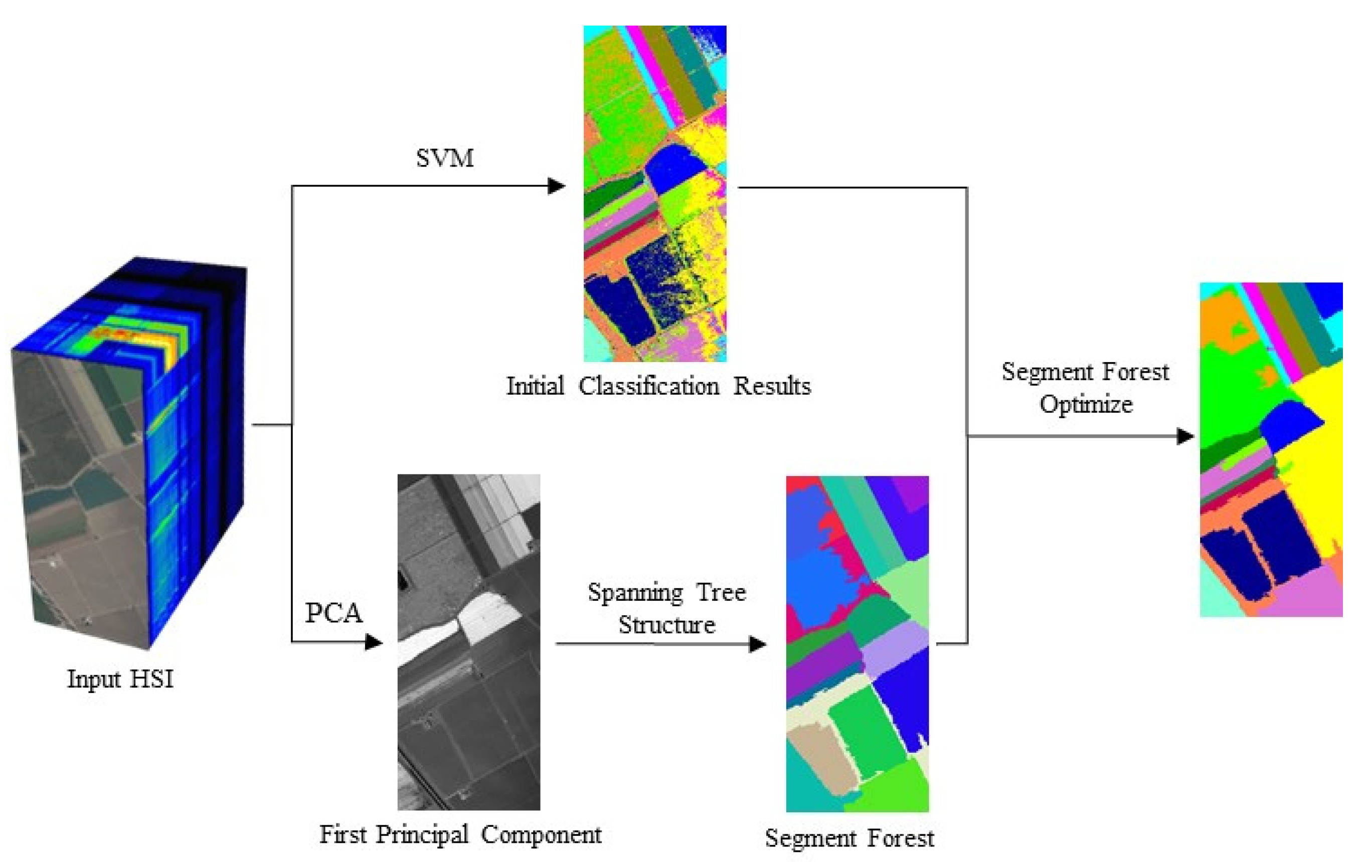
Segment forest is a tree-based classification method. The basic idea is to optimize the initial results by using the spatial information of the image. The main steps of segment forest are as follows:
  • Obtain the initial classification results. Part of the labeled data was extracted as training data and input into SVM to obtain the probability value of initial classification.
  • Obtain the first principal component of the original hyperspectral image. In order to improve the efficiency of the algorithm, principal component analysis (PCA) was used to project the original image hyperspectral data onto a new orthogonal space and extract the first main component.
  • According to the weights of the edges in the tree structure, the vertices are combined to construct a segment forest. The vertices are combined by calculating the weights of edges in the first principal component of the image. In order to prevent all vertices from merging into a single tree, the subtree is merged if the edge weight is less than a certain value. Finally, to prevent noise from affecting the subsequent result, subtrees with less than a fixed number of vertices in the tree are merged into the tree with the lowest weight.
  • Calculate the aggregation probability of vertices in the tree and determine the classification of each vertex. To carry out the filtering inside the independent tree of forest segmentation, not only to calculate the aggregation probability of each vertex, but also to complete the filtering from leaf to root and root to leaf and obtain the final classification result. Figure 2 shows the technical roadmap.

2.2.1. The Initial Classification Results

The basic idea of SVM is to solve the separation hyperplane, which can divide the training data set correctly and has the maximum geometric interval. Radial basis function (RBF) was used as the kernel function to classify the hyperspectral images in the experiment. Cross-validation was implemented using the LIBSVM software package to determine the optimal parameters C and Gamma values. Then the parameters were used to achieve the initial classification of hyperspectral images.
Suppose the size of HSI is H*W*B. The initial probability value obtained is a matrix, where the row data is the probability that the pixel point belongs to all labels:
M p k = P k ( i , j ) ;   i ϵ [ 1 ,   H ] ,   j ϵ [ 1 ,   W ] ,   k ϵ [ 1 ,   N ]
where, M p k is the probability that point (i,j) belongs to class K, and N is the maximum value of the label.
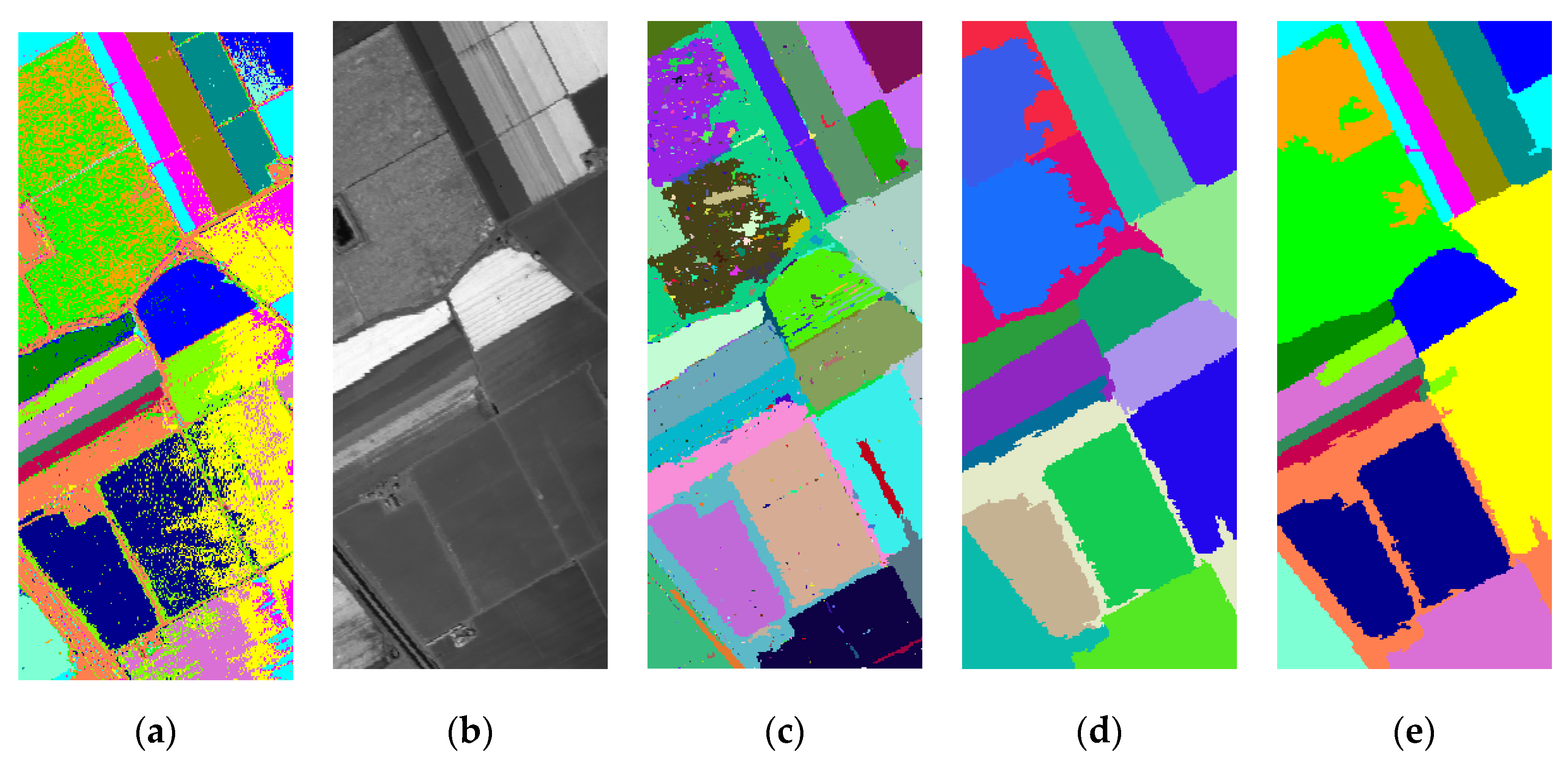
The label with the largest probability value of each pixel is assigned to the classification of this point. The visual result of the probability result is shown in Figure 3a.

2.2.2. Constituting the Segment Forest

There is a significant amount of spectral redundancy that exists in HSI data, so some level of signal compression or dimension reduction is appropriate [31]. The first principal component is also implemented by the PCA function of the Python scikit-learn library. n_components parameter is set to 1 to represent the first principal component of the extracted image. The image of the first principal component of Salinas is shown in Figure 3b.
On the other hand, a remote sensing image is usually stored in a grid structure, and the connection of the tree structure is beneficial to the algorithm to extract the spatial information of the image. Different from the graph structure, the tree structure has no closed loop connection. Each pixel in the first principal component is regarded as a vertex, denoting V, and the relationship between each pixel is considered to be an edge, indicating E, so that the first principal component can be expressed as G = { V ,   E } . The edge weight is expressed by the absolute value of the pixel value. That is, the weight of the two vertices in the image is ω e :
ω e = | x i x j |
where, x i and x j represent the pixel values of vertices.
Each pixel in the first principal component image obtained by HSI is regarded as an independent subtree. The weights of edges are sorted from smallest to largest, and the vertices with the weights from smallest to largest are joined to merge the subtree. A restriction (Formula 3) is added in merging the subtree to prevent all vertices from merging to one root node.
ω e min ( max ( ω T p ) + k V p , max ( ω T q ) + k V q ) )
where ω e is the weight of the edge between the subtrees Tp and Tq , V p and V q are the number of vertices in the subtrees p and q, and k is a constant parameter. In other words, if the coefficients between two subtrees meet certain conditions, they will be merged. This condition includes the coefficients of internal edges of each subtree and the number of internal vertices. It can be seen from Formula (2) that the number of vertices in a subtree is negatively correlated with the possibility of merging. That is, the more vertices in a subtree, the less likely it is to be merged. Under the limitation of Formula (2), some independent vertices must not be merged with other trees, resulting in some noise in the segment forest, as shown in Figure 3c. In order to prevent noise generated in segment forest from affecting the optimization results, the minimum number of vertices in subtrees is set to be no less than a certain number in this paper. If the number of vertices in subtrees is less than this threshold value, that is:
min ( V p ) < A
Then the subtree is merged into the tree with the smallest edge weight for the second filtering. Where, V p is the number of vertices in the subtree, and A is a constant parameter.
Finally, each tree generated is regarded as a complete segment forest, and a segment forest composed of segment trees is generated on the whole image. Figure 3d shows the segment forest constructed by Salinas, in which one color represents a segment tree in the forest. As can be seen from the results, segment forest provides another perspective of classification results based on the spatial information of the image.
In the previous part of this paper, subtrees are merged according to the weight of the edge, which is the generation process of the minimum spanning tree (MST). In this paper, two merge restrictions are added based on the MST so that the final segmentation results are a set of some trees, so it is named the segment forest.

2.2.3. Segment Forest Optimization Classification

In this paper, the essence of filtering is to calculate the aggregation probability of samples, that is, to modify the results of spectral classification by aggregating spatial information. Since the samples to be calculated are not necessarily two samples with edge connection, to calculate the spatial relationship of images, the weight function S ( p , q ) between the samples is first calculated. The weight function is composed of the edge of the path between the two samples. The formula is shown in (5):
S ( p , q ) = exp ( i ϵ path ( p , q ) ω ei γ )
where, ω ei is the weight of the edge connecting p and q, and γ is a constant parameter.
Then the aggregation probability M ¯ p d is:
M ¯ p d = q ϵ T q   S ( p , q ) M q d
T q is the segment tree where point q is located.
Filtering completes the part covered by each tree in the forest through filtering from leaf to root and from root to leaf.
Firstly, filtering from leaf to root is carried out. The formula is shown in (7):
M p d = M p d + q ϵ c ( p ) S ( p , q ) M q d
where c ( p ) is the set of child nodes of point q. Then, filtering from the root to the leaf,
M ¯ p d = S ( f ( p ) , p ) M ¯ f ( p ) d + ( 1 S 2 ( f ( p ) , p ) ) M q d
where f ( p ) is the parent node of p.
The filtering results of SF are shown in Figure 3e. Based on the initial classification results of SVM and combined with spatial information, the classification results are further optimized to obtain good classification results.

3. Results

3.1. Parameter Analysis

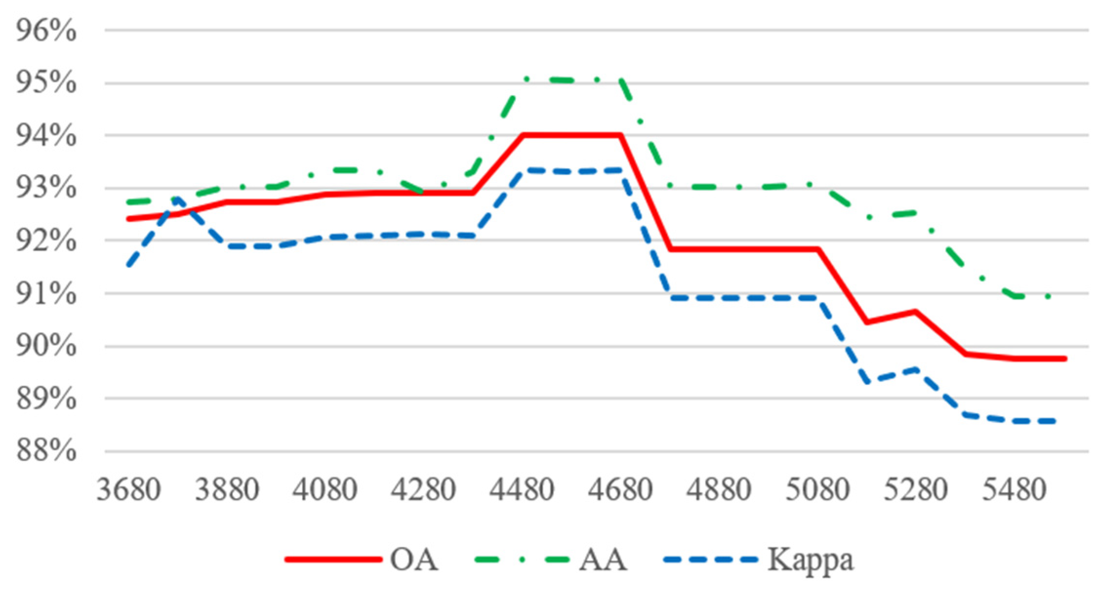
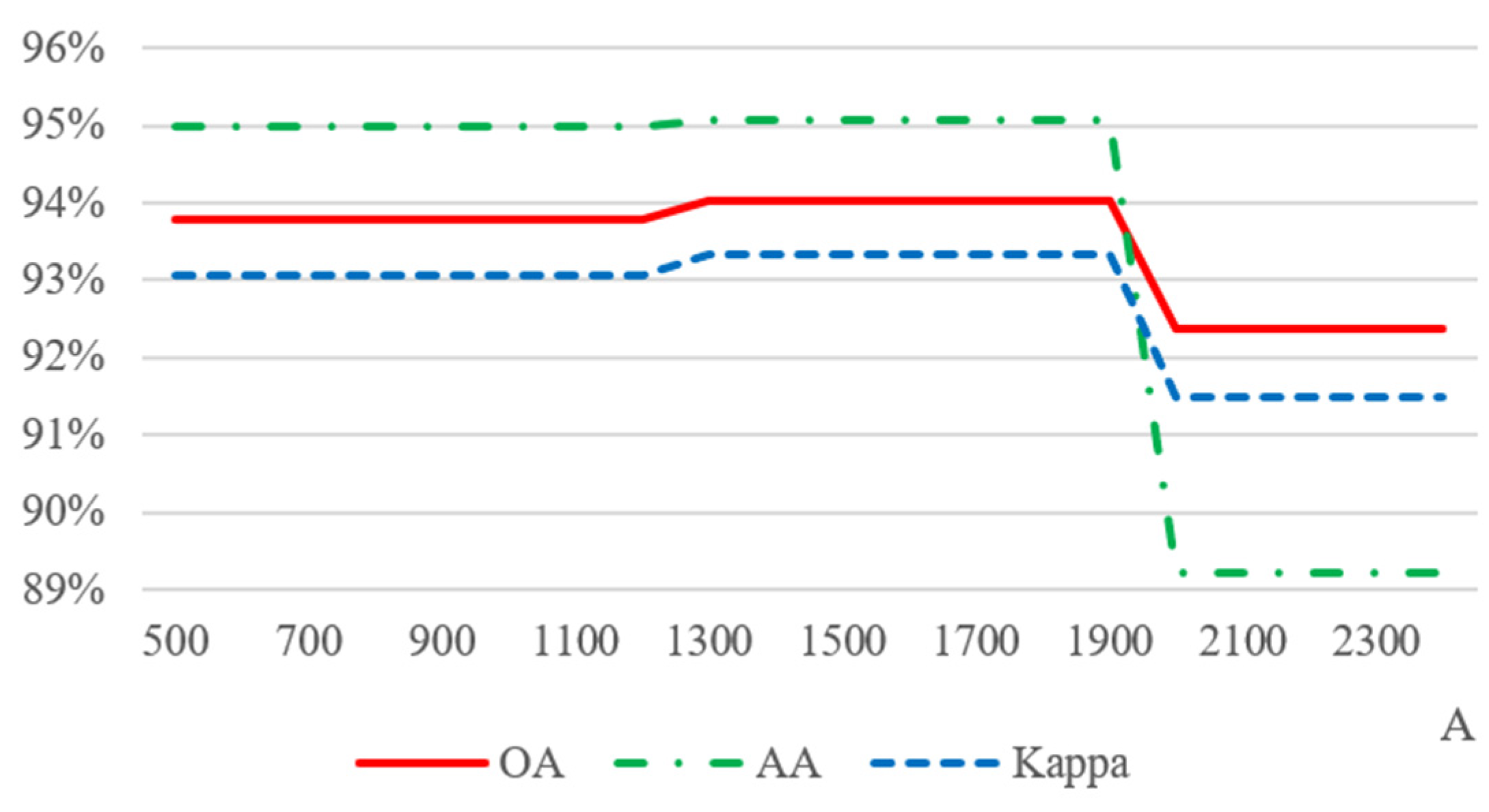
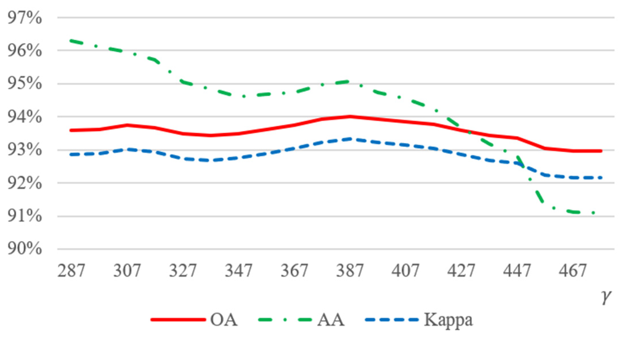
In this paper, there are three main parameters of image classification accuracy: K, A, and γ. K represents the possibility of merging subtrees, and the greater the value of K, the easier the merging will be. A represents the number of vertices in the tree with the fewest vertices in the partition forest. γ represents the influence between vertices in calculating the probability of aggregation. The smaller γ is, the less influence p has on q.
In order to verify the impact of parameters on the classification results, Salinas is mainly used to ascertain the effects of parameters on the results. When demonstrating the influence of parameter K on classification accuracy, parameter A is set to 1500 and parameter γ is set to 387. When verifying A and γ, the other two parameters are also set to fixed constants. The verification results are shown in Figure 4, Figure 5, and Figure 6. Parameter A and parameter γ have the most negligible impact on classification accuracy, and the curve fluctuation is slight, while parameter K significantly impacts the classification accuracy.

3.2. Influence of Training Data Set

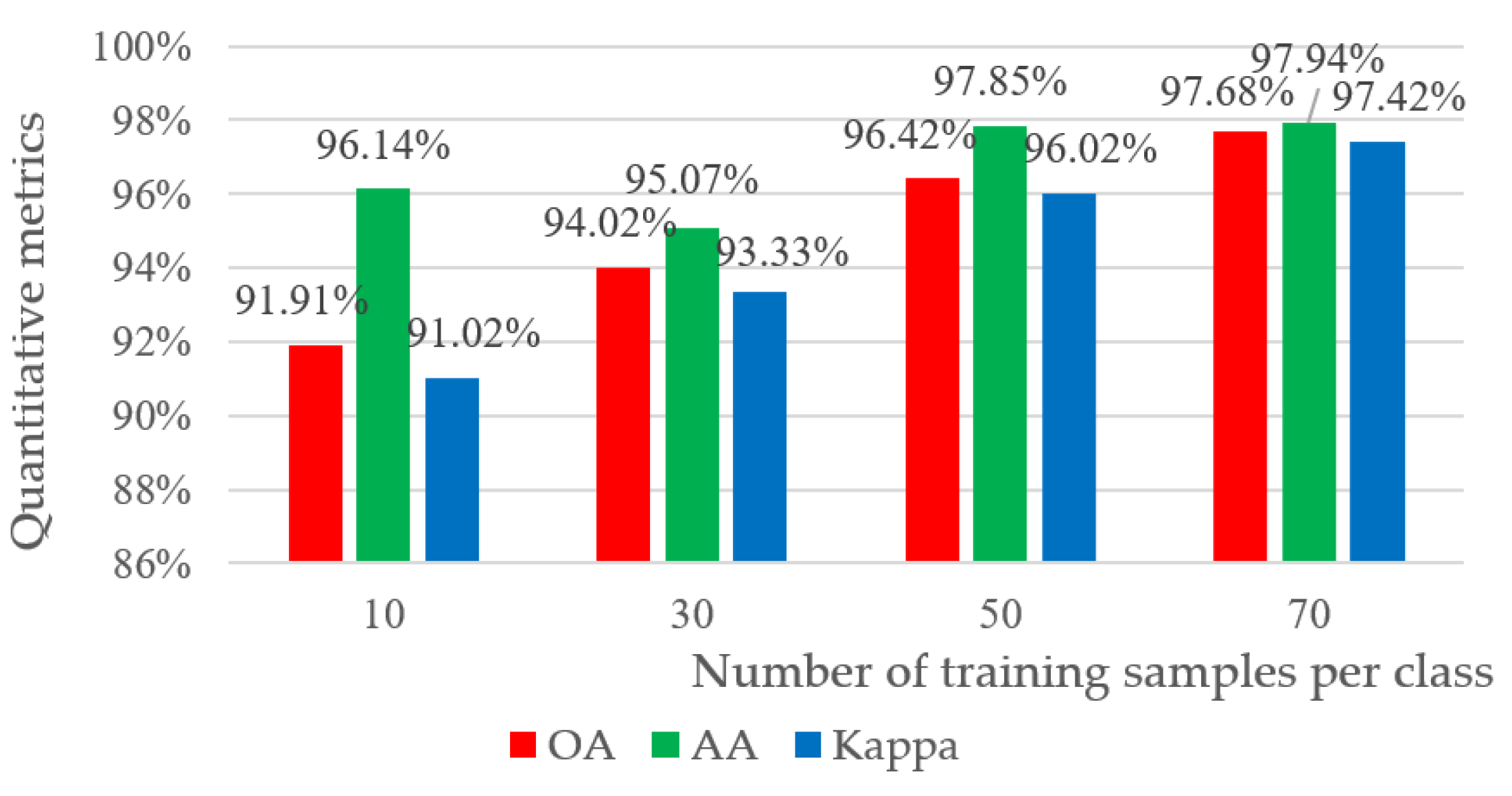
In this section, we discuss and evaluate the images of training samples on the accuracy of the SF method from two aspects. First, we evaluate how the number of training samples affects the classification accuracy of the proposed method. Figure 7 shows that training samples ranged from 10 points per category to 70 points per category. With the increase in the number of training samples, the classification accuracy increases. Moreover, when the number of training samples is small, SF can also achieve better optimization results based on initial classification.
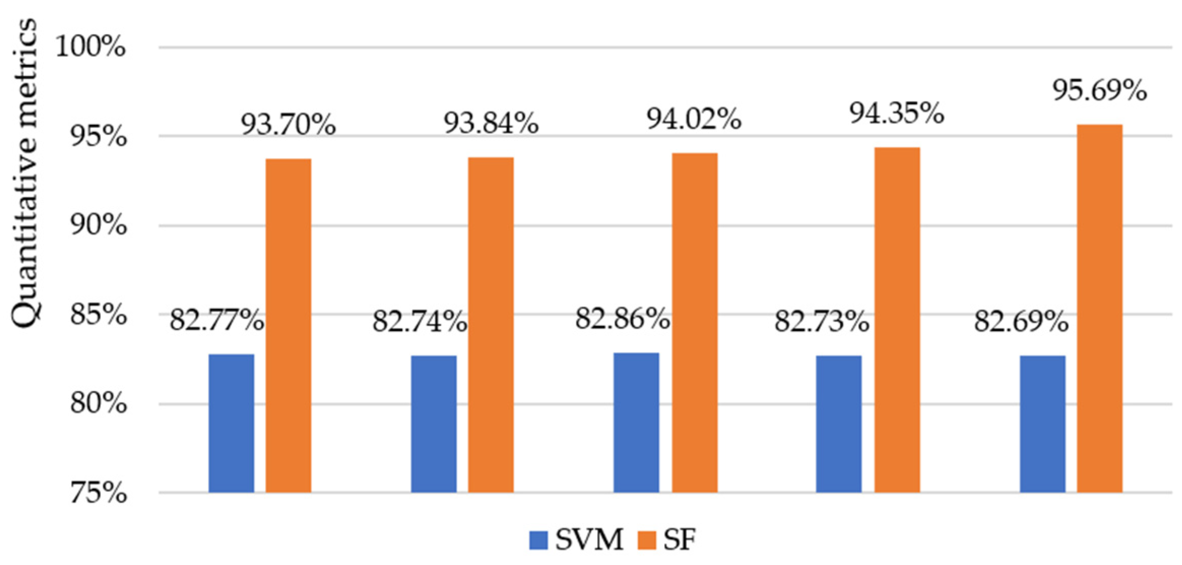
Secondly, we randomly select different sample points from the Salinas data set for training and analyze the classification accuracy of SF from the perspective of the randomness of samples.
As shown in Figure 8, after five times randomly selected training data sets and calculation of classification accuracy, it can be seen from the results that the classification accuracy of the SF method fluctuates slightly but remains within an acceptable range. The stability of the algorithm is proved. Additionally, in the process of parameter adjustment, when the constant parameter A value is in the range of 1300 to 1900, it maintains the highest classification accuracy. The other two parameters, K and γ, float only in small ranges. Therefore, it is speculated that the setting of constant parameters has a great relationship with the image itself (possibly the size of the classified object in the image or the size of the whole HSI image) but has little relationship with the selected training data or the spatial position of the vertex of the training data in the image.

3.3. Comparison of Different Spatial–Spectral Methods

This section mainly selects six improved spatial–spectral classification methods based on decision level and compares them with the SF. The main selected comparison experiment methods are divided into two categories: One is graph-based optimization methods such as GF, MRF, and RW, and the other is tree-based optimization methods such as MST, MST+ (this paper defines this method as the noisy filtering method of SF above), and ST. The above methods are based on the initial classification results of multi-classification SVM to optimize the final classification results further. Table 2 lists the data parameters in the figure.
The main advantage of GF is that the image edge retention effect is better and its primary parameter is the size of the filter window [18], which is related to the size of the classified target in the hyperspectral image. The window size used by GF in different hyperspectral images is also different. MRF, also known as the undirected graph model, mainly shows that pixels influence each other without apparent causality in the image. Each pixel has a certain connection with the surrounding points but has little influence on the pixels farther away. This is consistent with the actual spatial relationship in remote sensing images, so MRF performs well in image classification. However, the matrix-penalty factor matrix, which represents the relationship between pixels in the image, is challenging to obtain and has not formed a unified method. It is often determined independently according to specific models [32,33]. RW is a graph-based classification method whose basic idea is to extract spatial information according to the relationship of each edge in the image, corresponding to the possibility of random walkers crossing that edge. In the implementation of RW, large sparse linear equations need to be calculated [20]. Suppose the direct iterative method is used for calculation. In that case, a large amount of memory will be consumed, and even the existing hardware is difficult to meet the calculation requirements when the amount of data is large. To solve this problem, BiCGSTAB class in the Eigen library [34] is called in this paper, and the incompleteLUT preconditioner matrix is used to speed up convergence. As a global method, RW also has a relatively good performance in the aspect of accuracy. However, due to the complexity of the operation of the above matrix, there is a problem of low efficiency.
The minimum spanning tree (MST) is proposed to provide a way for us to analyze the connections between pixels to obtain spatial information. ST (segment tree) classification is based on MST, adding the condition of vertex merging. Many individual trees were generated on remote sensing images. Then merge all the subtrees in the graph into a single tree to form the segment tree. Then the segment tree is used to optimize the initial classification from the spectral information, and a good result is obtained. ST uses the tree structure to rearrange the spatial relations in the image, thus affecting the classification results of spectral information. However, ST still combines all vertices into a tree, and there are still interactions between different categories in the filtering process, thus affecting the final classification result. In this paper, inspired by ST, the classification of segment forest (SF) hyperspectral images is realized. SF is different from ST but regards the subtrees of MST with conditional constraints as independent trees, and then regards the whole image as a segment forest composed of trees. Finally, the independent trees in the segment forest are used to filter the initial classification results of the image regions covered by them. Experimental results show that the SF algorithm has better classification accuracy and computational efficiency than other spatial–spectral classification methods.
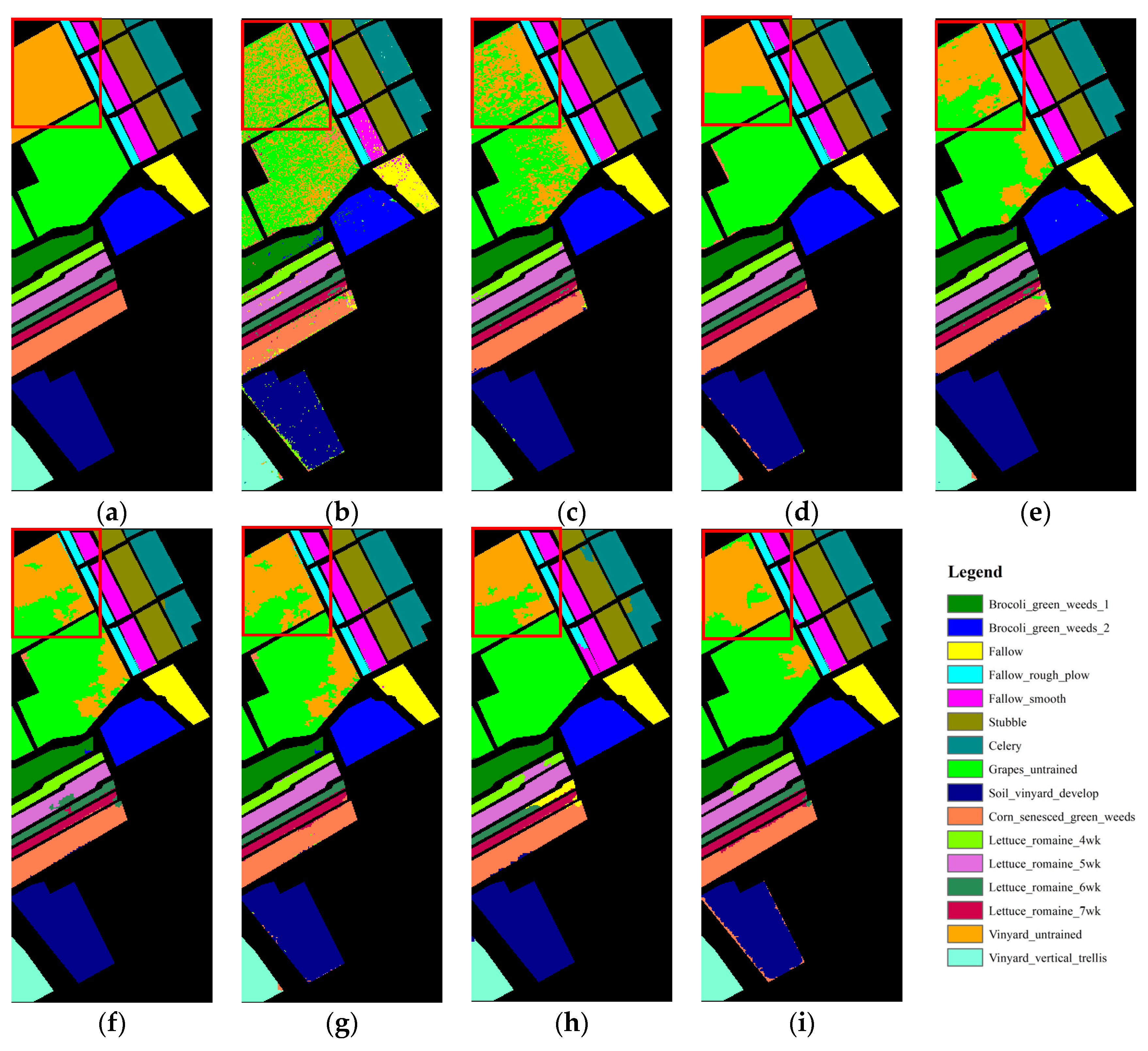
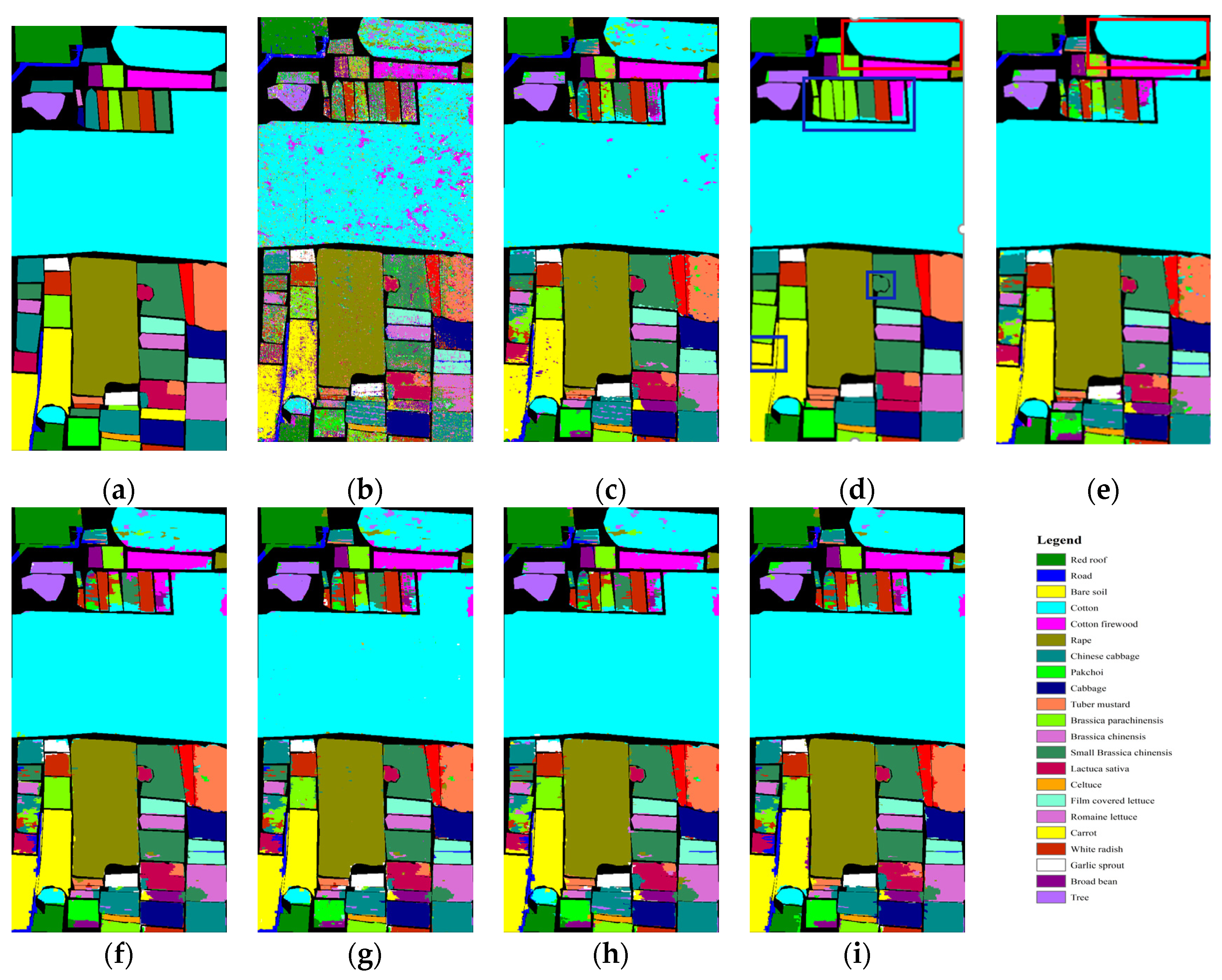
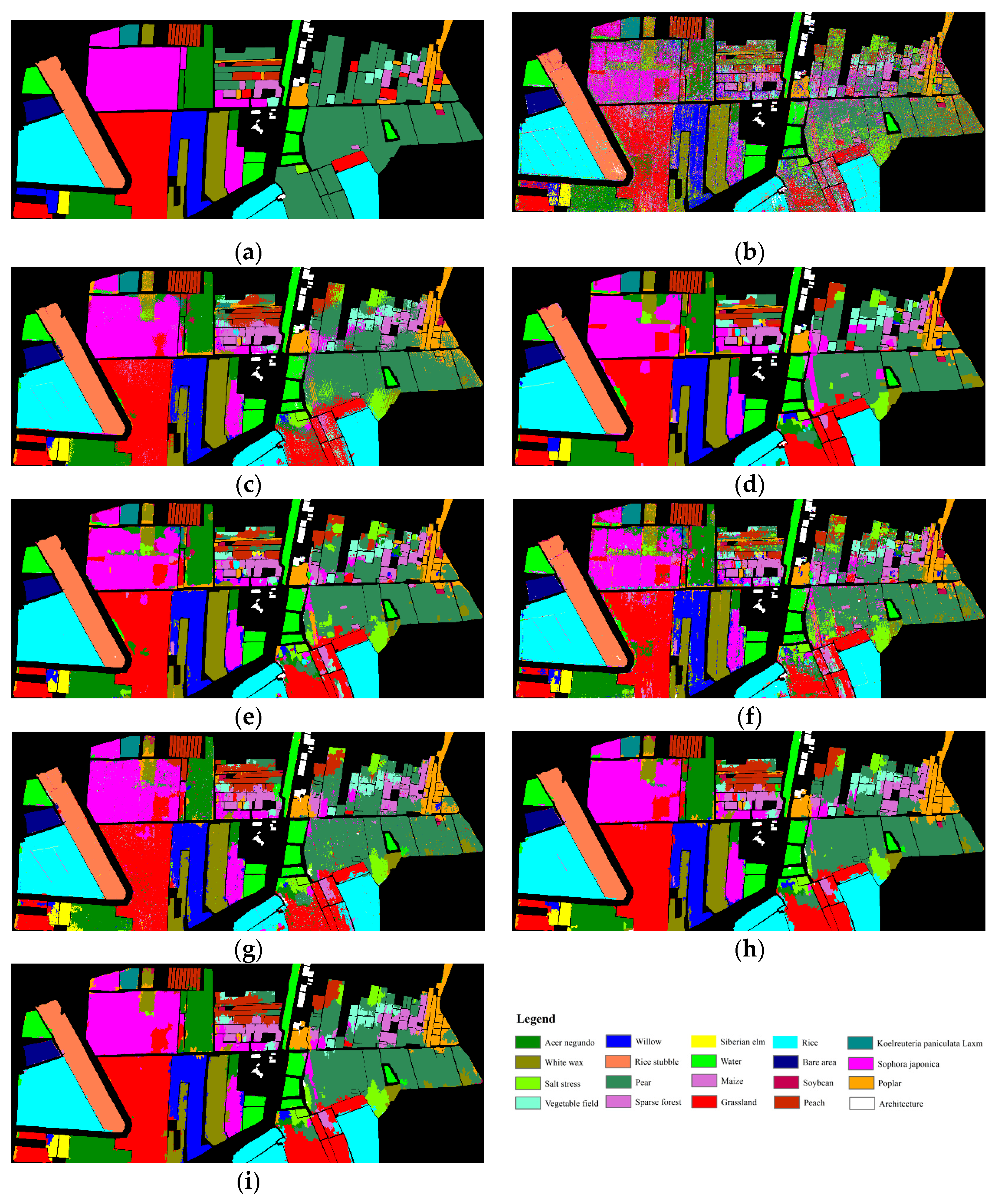
Three data sets are used in this paper to compare proposed method with other spatial–spectral methods, and the results are shown in Figure 9, Figure 10 and Figure 11. The above spatial–spectral methods all depend on the initial classification results. As shown in the red box in Figure 9, SVM classification results are poor. After adding spatial information, the above spatial–spectral methods also have unsatisfactory classification accuracy for the areas with poor classification results. In particular, the GF method showed a slight improvement in SVM results, but SF still offered the most potent error correction ability. As a global method, MRF and RW perform well in a large continuous classification area, as shown in the red box in Figure 10. However, when MRF classification areas are not uniform in size, small regions are easily swallowed by labels in large areas, resulting in classification errors, as shown in the blue box in Figure 10. As the trees constructed by MST and MST+ contain a lot of noise, the final filtering results obtained are also full of noise, as shown in Figure 9f,g.
Overall, SVM only uses spectral information to classify hyperspectral images, which produces a lot of noise, while the spatial–spectral method can suppress the noise to a certain extent. In addition to MST and MST+, other methods have a better effect on noise suppression. However, the spatial–spectral methods all depend on the initial classification results of support vector machines. Suppose the proportion of incorrect labels in the initial SVM classification in a certain region of the image is large. In that case, the classification results of these context-combined classification methods (except MRF) will also have severe errors in an extensive range.
The classification results of the three data sets are shown in Table 3, including overall accuracy, average accuracy, Kappa coefficient, and the time consumed in the process of using spatial information to optimize the image after the initial classification of SVM. All experiments were run on Intel(R) Core(TM) i7-8700 CPU @ 3.20ghz 3.19ghz processor. According to the classification results in Table 3, the SF proposed in this paper effectively improves the classification accuracy based on SVM. The overall accuracy of Salinas, WHU-Hi-HongHu, and XiongAn is improved by 11.16%, 15.89%, and 19.56%, respectively. Compared with other spatial–spectral classification methods, SF has achieved better results. In terms of algorithm efficiency, as shown in XiongAn in Table 3, SF effectively improves efficiency and has obvious advantages when the data volume is large.

4. Conclusions

In this paper, a spatial–spectral hyperspectral image classification method, segment forest, was proposed. In hyperspectral images, the first principal component is obtained through data dimension reduction, which forms segment forest, and the spatial information of the image is extracted. Then the initial results of SVM classification, namely the spectral information, are optimized to obtain the final classification results.
The experimental results show that the segment forest-based hyperspectral image classification improves the accuracy of hyperspectral image classification, which is better than the other spatial–spectral classification methods, such as GF, MRF, RW, MST, MST+, and ST, and has been verified on the three data sets. Secondly, the spatial–spectral classification method depends on the initial spectral classification results to a large extent. If the initial classification results have high accuracy, the spatial information optimization can be significantly improved, otherwise the optimization effect is poor. Therefore, the quality of the spectral classifier is vital to the spatial–spectral classification method. Finally, when the amount of hyperspectral data is largely increased, the computational efficiency of SF is also greatly improved, the larger the data set is, the more pronounced the efficiency advantage will be.
In the following research, we will further study the following two aspects. Firstly, other spectral classification methods and spatial information extraction methods will be studied to obtain the best classification effect. On the other hand, considering the rapid development of deep learning in remote sensing image classification in recent years, combining spatial information with deep learning will be applied to improve the classification accuracy of the algorithm.

Author Contributions

Conceptualization, J.L. and H.W.; methodology, J.L. and L.L.; validation, J.L. and L.L.; formal analysis, J.L.; data curation, J.L.; writing—original draft preparation, J.L.; writing—review and editing, H.W. and L.L.; project administration, H.W.; funding acquisition, H.W. All authors have read and agreed to the published version of the manuscript.

Funding

This research was funded by The National Natural Science Foundation of China (grant number 32071775) and Development Research Centre of Beijing New Modern Industrial Area (grant number JD2021001).

Institutional Review Board Statement

Not applicable.

Informed Consent Statement

Not applicable.

Data Availability Statement

The data used to support the findings of this study are available from the co-first author upon request.

Acknowledgments

We would like to thank the anonymous reviewers and editors for commenting on this paper.

Conflicts of Interest

The authors declare no conflict of interest.

References

  1. Poojary, N.; D’Souza, H.; Puttaswamy, M.R.; Kumar, G.H. Automatic target detection in hyperspectral image processing: A review of algorithms. In Proceedings of the International Conference on Fuzzy Systems & Knowledge Discovery, Changsha, China, 13–15 August 2016. [Google Scholar]
  2. Kalluri, H.R.; Prasad, S.; Bruce, L.M. Decision-level fusion of spectral reflectance and derivative information for robust hyperspectral land cover classification. IEEE Trans. Geosci. Remote Sens. 2010, 48, 4047–4058. [Google Scholar] [CrossRef]
  3. Klaus, A.; Sormann, M.; Karner, K. Segment-based stereo matching using belief propagation and a self-adapting dissimilarity measure. In Proceedings of the 18th International Conference on Pattern Recognition, Hong Kong, China, 20–24 August 2006. [Google Scholar]
  4. LU, D.; Weng, Q. A survey of image classification methods and techniques for improving classification performance. Int. J. Remote Sens. 2007, 28, 823–870. [Google Scholar] [CrossRef]
  5. Melgani, F.; Bruzzone, L. Classification of hyperspectral remote sensing images with support vector machines. IEEE Trans. Geosci. Remote Sens. 2004, 42, 1778–1790. [Google Scholar] [CrossRef] [Green Version]
  6. Tuia, D.; Ratle, F.; Pacifici, F.; Kanevski, M.F.; Emery, W.J. Active learning methods for remote sensing image classification. IEEE Trans. Geosci. Remote Sens. 2009, 47, 2218–2232. [Google Scholar] [CrossRef]
  7. Böhning, D. Multinomial logistic regression algorithm. Ann. Inst. Statal Math. 1992, 44, 197–200. [Google Scholar] [CrossRef]
  8. Ratle, F.; Camps-Valls, G.; Weston, J. Semisupervised neural networks for efficient hyperspectral image classification. IEEE Trans. Geosci. Remote Sens. 2010, 48, 2271–2282. [Google Scholar] [CrossRef]
  9. Yi, C.; Nasrabadi, N.M.; Tran, T.D. Hyperspectral image classification via kernel sparse representation. IEEE Trans. Geosci. Remote Sens. 2013, 51, 217–231. [Google Scholar]
  10. Gittins, R. Canonical Analysis: A Review with Applications in Ecology; Springer: Berlin/Heidelberg, Germany, 1985. [Google Scholar]
  11. Du, Q.; Fowler, J.E. Hyperspectral image compression using JPEG2000 and principal component analysis. IEEE Geosci. Remote Sens. Lett. 2007, 4, 201–205. [Google Scholar] [CrossRef]
  12. Li, C.H.; Kuo, B.C.; Lin, C.T. LDA-Based Clustering Algorithm and Its Application to an Unsupervised Feature Extraction. IEEE Trans. Fuzzy Syst. 2011, 19, 152–163. [Google Scholar] [CrossRef]
  13. Jia, X.; Kuo, B.C.; Crawford, M.M. Feature mining for hyperspectral image classification. Proc. IEEE 2013, 101, 676–697. [Google Scholar] [CrossRef]
  14. Vandenbroucke, N.; Porebski, A. Multi color channel vs. multi spectral band representations for texture classification. In Pattern Recognition. ICPR International Workshops and Challenges; Springer: Cham, Switzerland, 2021. [Google Scholar]
  15. Le-fei, Z.; Bo, D.; Liang-pei, Z.; Zeng-mao, W. Based on texture feature and extend morphological profile fusion for hyperspectral image classification. Acta Photonica Sin. 2014, 43, 810002. [Google Scholar]
  16. Fang, L.; Li, S.; Kang, X.; Benediktsson, J.A. Spectral–spatial hyperspectral image classification via multiscale adaptive sparse representation. IEEE Trans. Geosci. Remote Sens. 2014, 52, 7738–7749. [Google Scholar] [CrossRef]
  17. Li, W.; Chen, C.; Su, H.; Du, Q. Local binary patterns and extreme learning machine for hyperspectral imagery classification. IEEE Trans. Geosci. Remote Sens. 2015, 53, 3681–3693. [Google Scholar] [CrossRef]
  18. Kang, X.; Li, S.; Benediktsson, J.A. Spectral–spatial hyperspectral image classification with edge-preserving filtering. IEEE Trans. Geosci. Remote Sens. 2014, 52, 2666–2677. [Google Scholar] [CrossRef]
  19. Li, W.; Prasad, S.; Fowler, J.E. Hyperspectral image classification using gaussian mixture models and markov random fields. IEEE Geosci. Remote Sens. Lett. 2013, 11, 153–157. [Google Scholar] [CrossRef] [Green Version]
  20. Grady, L. Multilabel random walker image segmentation using prior models. In Proceedings of the Computer Vision and Pattern Recognition (CVPR 2005), San Diego, CA, USA, 20–26 June 2005. [Google Scholar]
  21. Makantasis, K.; Karantzalos, K.; Doulamis, A.; Doulamis, N. Deep supervised learning for hyperspectral data classification through convolutional neural networks. In Proceedings of the 2015 IEEE International Geoscience and Remote Sensing Symposium (IGARSS), Milan, Italy, 26–31 July 2015. [Google Scholar]
  22. Patel, H.; Upla, K.P. A shallow network for hyperspectral image classification using an autoencoder with convolutional neural network. In Multimedia Tools and Applications; Springer: Boca Raton, USA, 2021; pp. 1–20. [Google Scholar]
  23. As, A.; St, A. Deep neural networks-based relevant latent representation learning for hyperspectral image classification. Pattern Recognit. 2021, 121, 108224. [Google Scholar]
  24. Cao, X.; Zhou, F.; Xu, L.; Meng, D.; Xu, Z.; Paisley, J. Hyperspectral image classification with markov random fields and a convolutional neural network. IEEE Trans. Image Process. 2018, 27, 2354–2367. [Google Scholar] [CrossRef] [Green Version]
  25. Yao, X.; Li, G.; Xia, J.; Jin, B.; Zhu, D. Enabling the big earth observation data via cloud computing and dggs: Opportunities and challenges. Remote Sens. 2019, 12, 62. [Google Scholar] [CrossRef] [Green Version]
  26. Shuai, Y.; Xyab, C.; Dzab, C.; Dla, B.; Lin, Z.; Gya, B.; Bgab, C.; Jyab, C.; Wyab, C. Large-scale crop mapping from multi-source optical satellite imageries using machine learning with discrete grids. Int. J. Appl. Earth Obs. Geoinf. 2021, 103, 102485. [Google Scholar]
  27. Cheriton, D.; Tarjan, R.E. Finding minimum spanning trees. Siam J. Comput. 1976, 5, 724–742. [Google Scholar] [CrossRef]
  28. Li, L.; Wang, C.; Chen, J.; Ma, J. Refinement of hyperspectral image classification with segment-tree filtering. Remote Sens. 2017, 9, 69. [Google Scholar] [CrossRef] [Green Version]
  29. Yza, D.; Xin, H.A.; Chang, L.A.; Xw, B.; Ji, Z.C.; Lz, A. WHU-Hi: UAV-borne hyperspectral with high spatial resolution (H2) benchmark datasets and classifier for precise crop identification based on deep convolutional neural network with CRF—ScienceDirect. Remote Sens. Environ. 2020, 250, 112012. [Google Scholar]
  30. Cen, Y.; Zhang, L.; Zhang, X.; Wang, Y.; Qi, W.; Zhang, P. Aerial hyperspectral remote sensing classification dataset of Xiongan New Area(Matiwan Village). J. Remote Sens. 2020, 24, 10–17. [Google Scholar]
  31. Farrell, M.D., Jr.; Mersereau, R.M. On the impact of PCA dimension reduction for hyperspectral detection of difficult targets. IEEE Geosci. Remote Sens. Lett. 2005, 2, 192–195. [Google Scholar] [CrossRef]
  32. Cao, P. Automatic Segmentation Algorithm for Magnetic Resonance Imaging Based on Improved MRF Parameter Estimation; Zhejiang University: Zhejiang, China, 2013. [Google Scholar]
  33. Sun, H.; Wang, W. A new algorithm for unsupervised image segmentation based on D-MRF model and ANOVA. In Proceedings of the IC-NIDC 2009, IEEE International Conference on Network Infrastructure and Digital Content, Beijing, China, 6–8 November 2009. [Google Scholar]
  34. Eigen. Available online: https://eigen.tuxfamily.org/index.php?title=Main_Page (accessed on 8 November 2021).
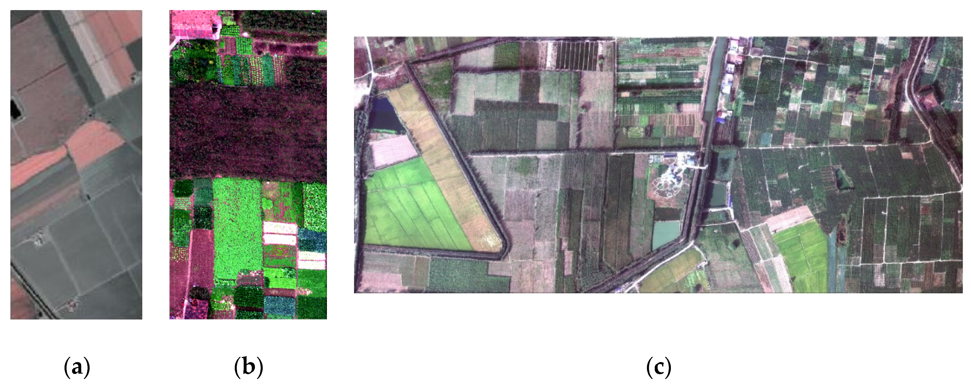
Figure 1. Three data sets used in this paper: (a) Salinas; (b) WHU-Hi-HongHu; (c) XiongAn.
Remotesensing 13 04816 g001
Figure 2. Technical roadmap.
Remotesensing 13 04816 g002
Figure 3. Salinas data set classification and segment forest optimization: (a) SVM probability distribution; (b) the first principal component image of Salinas; (c) noisy segment forest; (d) segment forest; and (e) results of segment forest optimization.
Remotesensing 13 04816 g003
Figure 4. Impact of parameter K on classification accuracy.
Remotesensing 13 04816 g004
Figure 5. Influence of parameter A on classification accuracy.
Remotesensing 13 04816 g005
Figure 6. Impact of γ on classification accuracy.
Remotesensing 13 04816 g006
Figure 7. Classification accuracy of Salinas with the different number of training samples.
Remotesensing 13 04816 g007
Figure 8. The overall accuracy of randomly selected training set (five times) of Salinas data set.
Remotesensing 13 04816 g008
Figure 9. Salinas’ (a) ground-truth and classification obtained by spatial–spectral method. The methods are: (b) SVM; (c) GF; (d) MRF; (e) RW; (f) MST; (g) MST+; (h) ST; (i)SF.
Remotesensing 13 04816 g009
Figure 10. WHU-Hi-HongHu’s (a) ground-truth and classification obtained by spatial–spectral method. The methods are: (b) SVM; (c) GF; (d) MRF; (e) RW; (f) MST; (g) MST+; (h) ST; (i) SF.
Remotesensing 13 04816 g010
Figure 11. XiongAn’s (a) ground-truth and classification obtained by spatial–spectral method. The methods are: (b) SVM; (c) GF; (d) MRF; (e) RW; (f) MST; (g) MST+; (h) ST; (i) SF.
Remotesensing 13 04816 g011
Table 1. Details of the hyperspectral image data set used in the experiment.
BandsImage SizeSpatial ResolutionFeature ClassesNumber of Training Samples per Class
Salinas224512 × 2173.7 m1630
WHU-Hi-HongHu [29]270940 × 4750.043 m22100
XiongAn [30]2563750 × 15800.5 m20100
Table 2. Parameters of segment forest experiment.
SF ParameterSalinasXiongAnWHU-Hi-HongHu
K4680200002630
A150016000710
γ3871490115
Table 3. Statistics of hyperspectral image classification results.
Data SetEvaluation IndexSVMGFMRFRWMSTMST+STSF
SalinasOA82.86%88.13%93.72%90.87%90.50%90.99%92.54%94.02%
AA90.72%94.29%96.67%95.31%95.03%95.66%91.26%95.07%
Kappa80.96%86.78%92.98%89.82%89.41%89.96%91.66%93.33%
Time(s)\3.1940.3727.360.3680.3330.3170.283
WHU-Hi-HongHuOA75.87%90.82%91.44%91.48%91.01%90.95%90.86%91.76%
AA72.95%89.15%87.97%86.12%87.88%87.50%87.26%87.79%
Kappa70.65%88.45%89.20%89.18%88.67%88.60%88.46%89.59%
Time(s)\17.9705.92256.8603.5871.2811.1620.709
XiongAnOA61.15%79.28%80.08%79.40%74.10%78.83%80.59%80.71%
AA72.62%84.56%91.21%90.45%86.85%84.12%84.87%82.46%
Kappa57.17%76.77%77.66%76.98%71.21%76.27%78.23%78.35%
Time(s)\207.295261.480842.326445.68442.69159.70636.571
Publisher’s Note: MDPI stays neutral with regard to jurisdictional claims in published maps and institutional affiliations.