Abstract
Crop rotations, the farming practice of growing crops in sequential seasons, occupy a core position in agriculture management, showing a key influence on food security and agro-ecosystem sustainability. Despite the improvement in accuracy of identifying mono-agricultural crop distribution, crop rotation patterns remain poorly mapped. In this study, a hybrid convolutional neural network (CNN) and long short-term memory (LSTM) architecture, namely crop rotation mapping (CRM), were proposed to synergize the synthetic aperture radar (SAR) and optical time series in a rotational mapping task. The proposed end-to-end architecture had reasonable accuracies (i.e., accuracy > 0.85) in mapping crop rotation, which outperformed other state-of-the-art non-deep or deep-learning solutions. For some confusing rotation types, such as fallow-single rice and crayfish-single rice, CRM showed substantial improvements from traditional methods. Furthermore, the deeply synergistic SAR-optical, time-series data, with a corresponding attention mechanism, were effective in extracting crop rotation features, with an overall gain of accuracy of four points compared with ablation models. Therefore, our proposed method added wisdom to dynamic crop rotation mapping and yields important information for the agro-ecosystem management of the study area.
1. Introduction
Crop rotation is the sequential growth of crops in a year [1] and has been practiced for thousands of years, serving as one of the most effective ways to increase grain yields [2,3]. Additionally, a crop rotation system is believed to have profound advantages over a monoculture cropping system for improving cropland fertility and mitigating weeds and pest insects [4]. Reliable and timely rotation maps are therefore fundamentally critical and can serve as essential inputs in monitoring cropping activity and agro-ecosystem fluxes for the purpose of good management practice and sustainability [5]. Nevertheless, spatio–temporal data on crop types and crop rotations at the field level for regional scales are rarely available, thus preventing further spatial explicit assessment and analysis [6,7]. Most regional or global studies have to rely on the assumption of a few simplified prototype crop rotations, bringing large uncertainty to evaluation results [4].
There have been a rather limited number of studies that attempted to derive crop rotation maps compared to the conventional single-season crop mapping. Mapping crop rotation not only requires precise discrimination of independent crop type during each growing season but also needs to capture dynamic changes of crop replacement. Previously, most studies have generated rotation maps based on spatial overlay analysis of single-season crop mapping results [8,9], i.e., to integrate rotation types by overlaying separate classification results from different years and summarize representative rotation patterns. Alternatively, other studies set rules and determined absolute thresholds to separate different crops step by step and finally acquire rotation maps [10,11]. In reality, however, rotation occurs seasonally and the integration of crop distribution maps could miss critical cross-seasonal crop dynamic information. In addition, pre-defined temporal thresholds often fail to accurately extract all rotation types at one time due to the spectral–temporal confusion of different crops and flexibility of the farmer’s planting behavior, especially in complex farming practice environments [12]. Thus, it is difficult to identify mono-agricultural patterns for various crops, let alone the cross-season rotational information for dynamic crop mapping.
Crop rotation is the temporal alteration of crop types, which could theoretically be captured directly with earth-observation satellites. Remote sensing imagery with time series has been widely used in mono-crop mapping because its enriched temporal information provides better performance than single-date satellite observations. From the time series of vegetation indices (VIs), the importance of phenological characteristics has been tested and emphasized to generate static crop maps by amplifying unique phenological phases of the target crop (e.g., transplanting, heading, and harvesting) [13]. Some of them incorporate phenological information by feeding statistical values (mean, standard deviation, etc.) of VIs on targeted dates or derived metrics from temporal profiles (amplitude, length, etc.) into unsupervised classifiers such as decision trees [14,15] and machine learning algorithms [16,17,18,19,20]. Others propose specific indexes to fully extract phenological information that is different from other crops [21]. However, such methods ignore successive crop growth with recursive temporal patterns and only treat temporal profiles, essentially, as unconnected segments. These empirical input variables greatly rely on subjective expert knowledge on crop phenology and possibly miss some subtle, but potentially critical, temporal signals with curve-fitted, time-series data. Other methods such as dynamic time warping (DTW) and time-weighted dynamic time warping not only focus on separate temporal characteristics but also account for the seasonality of crops reflected in the shape of the VI time-series curves, which are based on similarity measurements towards standard profiles, thus further improving upon the classification accuracy [22,23,24]. Theoretically, time-series information embedded in VIs not only enables the differentiation of certain crop types among others but also provides recursive crop rotation signals related to seasonal changes. However, the above traditional methods are only suitable for identifying single-season crop types and make it difficult to accurately excavate crop seasonal changes, let alone crop rotation information.
Recent advances in deep learning hold considerable promise for exploring intricate and high-dimensional relationships from end-to-end neural networks [25]. Over the past several years, an increasing number of studies have been performed using deep learning models for single-season crop classification [26]. For instance, one-dimensional convolutional layers (Conv1D) have been adopted for multi-temporal, crop-type classification, and have shown great potential in automatic multi-level feature extraction [27,28]. While the recurrent neutral network (RNN) has proven to be well suited for dealing with long sequential data such as sequences of VIs reflecting crop growth cycles [29]. Long short-term memory (LSTM), one of the most popular variants of RNN, has been successfully leveraged to recognize contextual information to produce crop maps [30,31]. Considering the loss of optical data due to persistent clouds, extra data sources, such as SAR, have been widely used in crop classification to fill optical data absence [32,33]. In this scope, multi-source remote sensing data provide complementary information and have the potential to extract complex dynamic features. Considering that the correspondence between SAR and optical time series is difficult to find, deep learning models are applied to interact at deep levels based on multiple sensors. Few studies have investigated the potential of multi-source data fusion by deep learning networks before classification [34,35]. Models with two structurally identical streams have been introduced to learn the relationships across sensors and test the effect in useful temporal feature extraction [36]. Although the up-to-date studies have suggested its competitive advantages in boosting crop mapping tasks by utilizing multi-temporal data from diverse sensors using hybrid deep learning networks [37], current crop mapping techniques mainly rely on stand-alone sensors without realizing deep synergy, while most of them allocate equal attention to each timestamp [38], which is not conducive to extract flexible crop rotation information. Moreover, the existing methods mainly focus on the extraction of stable land cover information rather than varied and complex cropland changes that occur over a year. The method of accurately identifying cross-seasonal changes and capturing dynamic patterns during a year to produce reliable crop rotation maps is still a big challenge.
The temporal feature of a satellite image time series contains abundant information, which can be used not only for the classification of static crop distribution but also for the sequential information of crop rotation. In this study, we propose a crop rotation mapping (CRM) model by integrating Sentinel-1 and -2 time series with the help of a deep learning algorithm. To achieve this, we employ a hybrid CNN-LSTM structure with an attention mechanism to extract hierarchical rotation features and further depict rotation temporal patterns. The main contributions of this work include:
- (1)
- A new hybrid deep learning network, proposed to capture both crop types and seasonal changes for crop rotation mapping;
- (2)
- Test results validating the advantage of a synergy SAR-optical time series and incorporating the use of the attention mechanism in LSTM over traditional and ablation models.
2. Study Area and Materials
2.1. Study Area
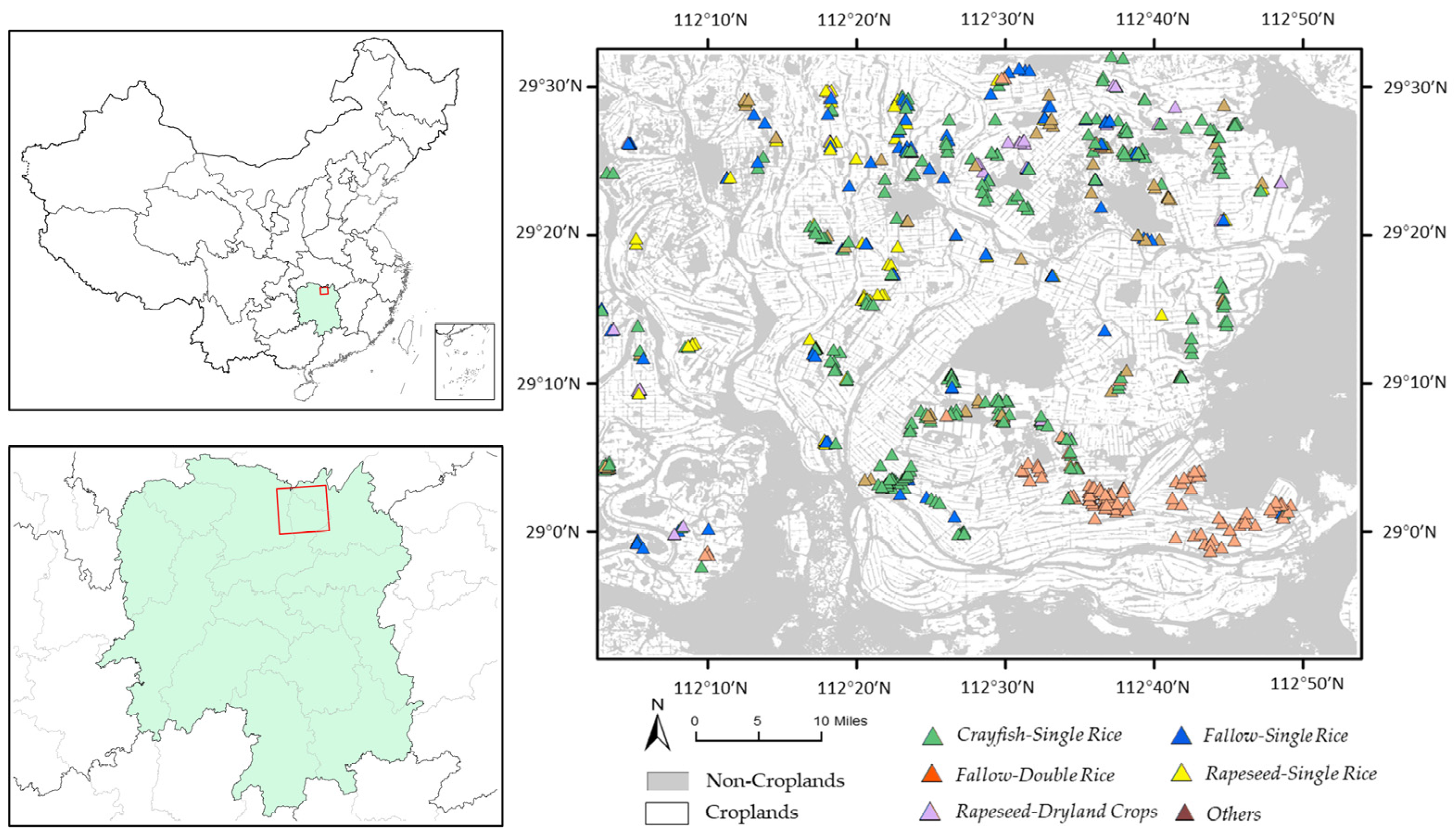
This research was conducted in the northern part of Hunan Province, central China, one of the largest rice-producing provinces in China (Figure 1). The study area was a flat fluvial plain (112.04 E–112.89 E, 28.86 N–29.53 N) south of the Yangtze River, and west of the Dongting Lake, with a total area of 7099 km2. It has a typical subtropical, humid monsoon climate with an abundant active accumulated temperature and annual rainfall of 1200 to 1900 mm.
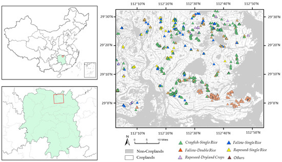
Figure 1.
Study area and ground truth distribution in Hunan Province, central China.
Abundant rainfall supports large areas of paddy and pond systems in this region. Rice is the major summer crop in the paddy system in this region, including both single-season rice (SR, May–Oct) and double-season rice (DR, Apr–Jul and Aug–Oct). Rotated within the rice plantation, local producers either left their land fallow for the rest of the year or grew rapeseeds (RS) as the winter cash crop (Nov–May, subsequent year). Another alternative was to use paddy fields as crayfish (CF) ponds in the spring, before the transplanting of single-season rice to increase farmer income. In addition to the rice-based rotation system, a smaller proportion of higher-elevated dryland was mainly used to grow summer crops such as maize, soybean, and cotton, which have very similar phenological stages as single-season rice. Dryland crops (DC) depend on the household needs of the individual and therefore are hard to further subdivide due to the diversity of types and them having almost the same phenology (Figure 2).

Figure 2.
S1 and S2 data acquisition date and phenological stages of primary rotation types with corresponding NDVI value averaged from ground truth samples in the growing season.
2.2. Satellite Data and Pre-Processing
Satellite image time series (SITS) of the Sentinel-1 synthetic aperture radar (SAR, S1) and Sentinel-2 (optical, S2) between January 2019 and December 2019 were collected from Google Earth Engine (GEE) (Figure 2). Both datasets have a spatial resolution of 10 m with a UTM/WGS84 projection system.
For the optical dataset, considering the noise impact of cloud cover, only 14 cloudless or partially clouded S2 images were finally selected. At the same time, pre-processing was performed before calculating vegetation indices to restore actual surface reflectance, including radiation calibration and atmospheric correction. Clouds were removed by assisting with the corresponding S2 cloud probability dataset recommended by the GEE platform. Two commonly used vegetation indices, the normalized difference vegetation index (NDVI) and the enhanced vegetation index (EVI), and one recently developed spectral index, the kernel normalized difference vegetation index (kNDVI), were used for rotation classification. NDVI and EVI time series have been widely used to extract phenological features of different crops [18,39], while kNDVI has proven to have a higher sensitivity to vegetative biophysical and physiological parameters compared to classical vegetation indices [40]. The three indices are computed as follows:
where and are the surface reflectance of band 8, band 4, and band 2 in the Sentinel-2 MSI sensor. is a length-scale parameter to be specified in the particular application representing the sensitivity to vegetation sparsity. Here, we chose the average value to provide an operational version of the original index.
For the SAR dataset, we referred to 30 SAR ground range detected scenes that were recorded in interferometric-wide (IW) swath mode with dual polarization (VV+VH). Each scene was pre-processed using the following steps: (1) thermal noise removal, (2) apply orbit file, (3) radiometric calibration, (4) terrain correction using digital elevation datasets, and (5) conversion of the backscatter coefficient (δ) to logarithm decibels (dB). Only VH images were used in the following analyses. To ensure the smooth running of the neural network, min-max normalization was conducted to VH images to obtain a similar numerical distribution as optical images.
2.3. Ground-Truth Data
Field surveys were conducted to obtain the ground truth of crop rotation in the study area in May 2021. Each sampling site was recorded with its specific geographic location centered at the land parcel (as the same geographic coordinate system as the satellite data, WGS84), with a farmer interview stating crop rotation types during the past three years (2018–2020). Only parcels that have maintained stable crop rotation types for three consecutive years were recorded. In total, 689 available ground samples were collected after careful inspection and screening to ensure the spatial homogeneity of ground truth and integrity of rotation types (Figure 1). For classification, non-cropland samples were also added through visual interpretation on the high-resolution image of Google Earth (201 non-cropland samples in total).
Sample augmentation was conducted considering the demand for sample size and positioning uncertainty. Four pixels (top, bottom, left, and right) centered on each ground truth were obtained and assigned the identical crop rotation type as that at the center. Through sample augmentation, 4450-pixel samples were obtained and used as independent samples in model training. According to the distribution and proportion of rotation types in the study area, we summarized six main rotation types as a classification system (sorted by proportion): crayfish-single rice (CF-SR), fallow-single rice (F-SR), fallow-double rice (F-DR), rapeseed-single rice (RS-SR), rapeseed-dryland crops (RS-DC), and other rotation types, together with four non-rotation classes: water, mud flat, vegetation, and construction land. We considered all 10 categories for the initial modeling, but only compared and assessed the performance of crop rotation types.
3. Crop Rotation Mapping (CRM)
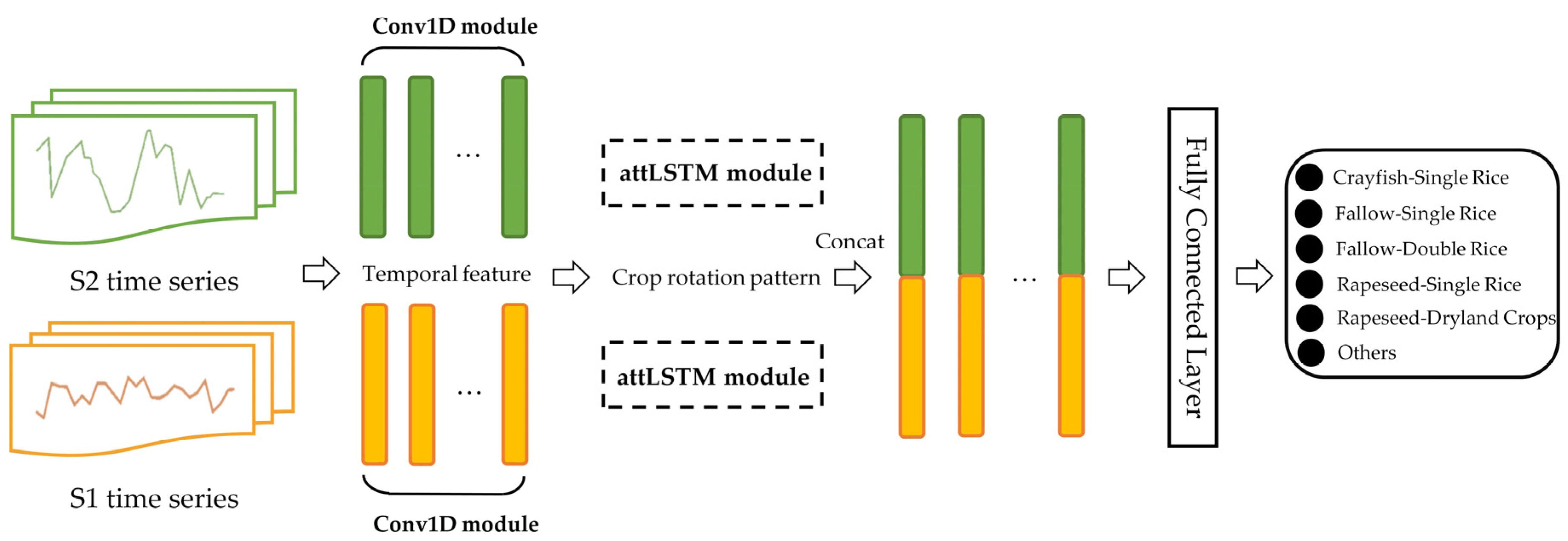
The proposed crop rotation mapping (CRM) has a hybrid architecture composed of two streams designed for each of the S1 and S2 time series (Figure 3). Each stream consists of two different neural networks: a one-dimensional CNN (Conv1D) and an LSTM with an attentive mechanism (AttLSTM). The Conv1D attempts to extract hierarchical rotation features, which involve a series of convolutional operations with alterable kernel sizes. The results of Conv1D enter into LSTM to depict temporal crop growing patterns assisting with an attentive layer. The output of each stream is a feature vector summarizing the extracted knowledge learned from the optical time series and SAR time series. The concatenation of the above two feature vectors is fed into the end module, which is operated by several fully connected layers activated by a nonlinear function helping to produce the final rotation decision.

Figure 3.
Structure of the proposed CRM. SAR and optical time series are fed to two separate streams. The Conv1D module is designed to extract temporal features, while the attLSTM module depicts crop rotation patterns. The output feature vectors from separate streams are concatenated to perform final crop rotation classification.
3.1. Robust Temporal Features Extraction with Conv1D
This operation was inspired by recent work [28], which successfully showed that the one-dimensional convolutional deep learning framework was capable of extracting effective and hierarchical features layer by layer in multi-temporal classification tasks.
In this study, we constructed two convolutional layers since convolution operations can be stacked to obtain abundant information from tiny to general. Two layers were equipped with different kernel sizes, which meant that the filter window covered different observations or learned features for all timestamps. The earlier layer focused on local features by using smaller sizes to capture minor changes, while the later layer summarized more general patterns on a larger time scale [28]. A Conv1D layer is represented by Equation (4).
where denotes convolution kernels, represents the number of kernels, represents bias, indicates the channel number, and indicates the activation function whereas * is the operator indicating convolution.
After the convolution layers, the max-pooling and dropout layers followed and helped in avoiding data dimensionality expansion. The dropout layer followed the first convolutional layer, whereas the max-pooling layer followed the second. Dropout is a regularization technique that randomly drops some neurons in a layer during training so that the output of the layer does not rely on only a few neurons [41]. The probability of dropping neurons was set considering the complexity of the model. The pooling layer was needed to ensure the progress of the further calculation. In this way, the output of Conv1Ds was a noise-adaptive feature that summarized useful crop rotation information and could be used as an input to the LSTM module.
3.2. Crop Rotation Patterns Depiction with LSTM
An LSTM unit was used to represent the growing characteristics of the rotation systems because of its outstanding performances in the area of remote sensing time series processing and analysis [42]. An LSTM unit is designed to “remember” and “distinguish” values according to formerly processed information in a long inherent sequence, the same as temporal profiles containing crop rotation information. The use of LSTM improves the effectiveness of depicting temporal patterns at various time intervals, which is promising to express rotation systems growing cycles with different frequencies.
An LSTM unit is composed of three main gates: forget, input, and output. The forget gate reserves previous information selectively and only focuses on essential signals, while the input and output gates (a gate represents a neural network containing sigmoid activation function) decide what information will be stored and exported in the current state. Each gate contains a sigmoid layer and a multiplication operation to contain both the state of the previous time step and the current input signal.
Equations (5)–(10) formally describe the LSTM interior working principle:
where represents the forget gate, denotes the input gate, is the output gate, and indicates a feature vector presenting the memory state, whereas is the weight vectors for all the four gates and represents the bias. denotes the time step.
3.3. Crop Rotation Mapping with a Multi-Temporal Attention Mechanism
After the attLSTM module, we coupled the output features with an attention mechanism. Attention mechanisms are widely used in automatic signal processing and they analyze the information extracted by a recurrent neural network model at different time stamps synthetically [43]. Intuitively, the attention mechanism supports the model to focus on the important part of the signal while discarding the useless portion of the information.
The output of LSTM cells was a sequence of learned feature vectors. The attention mechanism can be presented with the following equations:
where indicates the matching degree between the input of the encoder and the output of the decoder. is the hidden state, while is the output state. is called the alignment model.
The features derived from both LSTM and Conv1D architecture, enhanced by the attention mechanism from the SAR and optical multi-temporal imagery, were combined by concatenation techniques to synthesize complementary multi-source remote sensing information [36]. Regarding the output part, our model contained two fully connected layers at the end module. We adopted the second to last layer with the ReLU activation function to further collect information from the integrated results. The final layer contained as many neurons as the number of classification types to produce each class probability with a softmax activation function.
4. Experiments
Experiments were designed to test and compare the performance of our proposed CRM.
4.1. Competing Models and VIs
We focused on two different aspects of comparative analysis: (1) the performance of our proposed CRM vs. other classical and advanced models, and (2) the sensitivity of vegetation indices as model inputs.
Four competing models were considered:
- RF(S2): A random forest (RF) classifier with Sentinel-2 time series inputs was used to derive the baseline performance of classical non-deep learning architecture. RF has been considered as the most common and effective land cover mapping approach [44] because of its high performance in the classification task, combined with optical time-series data in recent mapping works.
- LSTM(S2): A deep learning classifier that used an LSTM unit with the attention mechanism with Sentinel-2 multi-temporal inputs, following the lead of popular frameworks [45,46]. To adopt such a model, we employed 14 Sentinel-2 images to the LSTM layer to capture dynamic growing information, plus an attention layer to allocate independent weight to each timestamp. Here, LSTM(S2) represented the baseline of time series processing with deep-learning architecture.
- CRM(S2): An ablation model that only considered the optical source, because optimal temporal profiles could better express crop rotation cycles and record crop growth compared to unexplainable SAR profiles. Such a structure was introduced not only to disentangle the benefits of convolutional operation compared to LSTM(S2) but also to demonstrate the necessity of synergizing multiple satellite sources compared to the original CRM model.
- CRM(NoAtt): An ablation model excluding the use of the attention mechanism. Here, CRM(NoAtt) was conducted to prove the importance of assigning weights according to different temporal characteristics.
Given our proposed CRM and four competing models, each of NDVI, EVI, and kNDVI was used in accordance, yielding 5 × 3 = 15 different model-VI combinations for the comparative test of performance in extracting crop rotation maps.
4.2. Model Training
When feeding our models, 80% of samples were randomly selected from the ground-truth collection for training, and the rest were used for validation. To avoid accuracy uncertainty due to random training and validation split, we applied a fixed set of the shuffled dataset to all competing models, which eliminated the risk of sample labels clustering in the near neighborhood.
In order to realize the maximum potential of the models, the selection of hyperparameters was performed step by step, based on experience. We started with a relatively simple model, then we generated new models by adding a new convolutional layer, re-ordering layers, or changing one or two hyperparameters, i.e., different types of activation functions, number of neurons, kernel size of convolutional layers, batch size, learning rate, and number of epochs. The one hyperparameter that no longer increased classification performance on accuracy was selected to produce final results. The above optimization procedure was applied to all four deep learning models. The RF model was trained by the tuning of the number of trees in the forest.
All deep learning models were trained by using the Adam optimizer with cross-entropy loss function, which has proven to be superior to other optimization methods, and it has been widely used in most time series classification tasks. Parameters of the Adam configuration were consistent with the recommended ones [47]: 1 × 10 −7, and the learning rate was fixed as 0.001. All deep learning models are implemented using the Python Tensorflow library, while random forest methods are processed by the Python Scikit-learn library. The number of trees was optimized at 100 at the end.
4.3. Model Evaluation
Model performance was evaluated by using accuracy indices and a confusion matrix that has been widely used in previous studies [36], including global and per-class accuracy, kappa coefficient, and F1 score. Accuracy is the most common evaluation metric in remote sensing and is calculated by dividing the sum of pixels correctly classified by the total number of pixels analyzed, intuitively showing the ability of the classifier to accurately predict targets. The kappa coefficient is a score that expresses the level of agreement between the actual and estimated targets on a classification problem. The F1 score can be interpreted as a harmonic average of precision and recall, where an F1 score also reaches its best at 1 and worst at 0. Here, we used the macro average of the F1 score as an indicator of classification capability, which assigns equal weights to all classes and does not take label imbalance into account.
5. Results
5.1. Sensitivity Analysis of VIs as Model Input
Different vegetation indices behaved differently in diverse models (Table 1). kNDVI showed a slight advantage over NDVI and EVI only when used with CRM, and achieved the highest accuracy of 0.876 among all models. By contrast, NDVI achieved an overall stable and preferable performance in the rotation mapping task and provided the best results in the two basic competing models RF(S2) and LSTM(S2), where there was a large gap between EVI and two kinds of NDVI. Interestingly, EVI outperformed the other two VIs in the ablation models of CRM, closely followed by NDVI.

Table 1.
Accuracy, F1 score, and kappa coefficients for different vegetation indices and competing methods.
5.2. Ablation Analysis of Multi-Source Data and Attention Mechanism
For each type of vegetation index, CRM outperformed three mono-source competing methods with an average accuracy of 0.87, therein, the random forest model obtained lower performance scores than the other two neural network structures. Its overall accuracy was about 0.74.
Full source classifiers (CRM) provided a superior capability compared to CRM(S2), using only an optical data source on crop rotation mapping. The progress was achieved with a precision promotion of four points. As expected, feeding the model with the full set of heterogeneous information promotes classification performance. Furthermore, CRM always outperformed CRM(NoAtt), noting gains in precision due to the allocation of greater weights to more important timestamps.
Table 2 reports F1 score performance of the different methods with their corresponding optimal vegetation indices input. Again, CRM outperformed all competing models in most rotation types except for rapeseed-single rice, where RF(S2) showed slightly better results. This is another example of our original intention to show that the adoption of a multi-source time series with specific attention to different stages of crop growth can effectively capture rotation features. It is also notable that CRM showed a substantial advantage over its single-source ablation variant (CRM(S2)) for all rotation classes, especially for the smallest proportion of rotation type (RS-DC) with an increase of 13 points, which cannot otherwise achieve excellent performance by other traditional models. Moreover, the attention mechanism played an important role in the classification of fallow-single rice, which is difficult for most competing models, where RF(S2) only had a 60% chance of successful identification. It showed a large promotion from 0.71 to 0.81 compared to CRM(NoAtt). It proved that CRM is qualified to better distinguish these objects with the help of deep mining of specific temporal characteristics.

Table 2.
F1 score per rotation type for best performance models.
We also investigated the confusion between each pair of rotation types for all methods with their corresponding optimal vegetation index (Figure 4). The visual results also supported the observations drawn from Table 2, as CRM was more precise than other competing methods, while RF(S2) exhibited relatively poor behavior reflected by the lower diagonal scores. Among the rotation classes, fallow-double rice and crayfish-single rice are most easily identified.
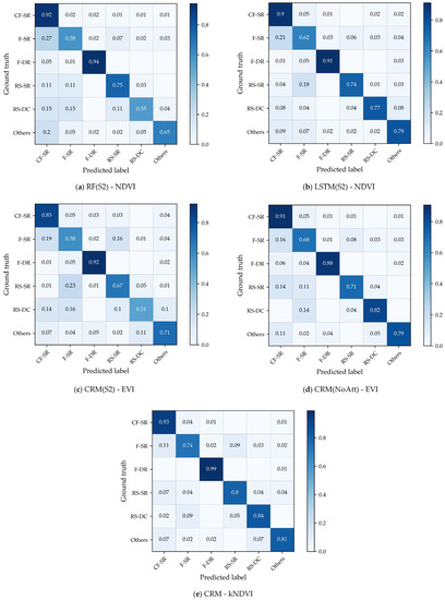
Figure 4.
Confusion matrixes for models along with the best-performing vegetation index. (a) RF(S2) using NDVI as input; (b) LSTM(S2) using NDVI as input; (c) CRM(S2) using EVI as input; (d) CRM(NoAtt) using EVI as input; and (e) CRM using kNDVI as input.
Slight confusion appeared among fallow-single rice, rapeseed-single rice, and crayfish-single rice. For instance, the RF(S2) model misclassified 27% of fallow-single rice as crayfish-single rice and CRM(S2) misclassified 23% of rapeseed-single rice with fallow-single rice. Farmers sometimes grow grass in crayfish-paddy fields to provide feeds, which creates challenges to distinguish between the early growing stage of rapeseed and fallow fields with wild grass before single rice sowing, even by manual visual interpretation on site. However, CRM took advantage of SAR data and leveraged the ability of the neural network in identifying the above three classes with an error below 0.1. Moreover, the performance of the proposed model was substantially improved in distinguishing summer paddy rice and dryland crops with the introduction of the attention mechanism. As shown by the difference between CRM(NoAtt) and CRM, up to 14% of dryland summer crops were misclassified as single rice rotations (RS-DC and F-SR). The confusion between single rice and dryland crops has been largely reduced in the RS-DC, RS-SR, and F-SR rotation systems in CRM models, which owns quite similar phenological progress. The confusion between RS-DC and RS-SR remained relatively low (0.05) in CRM.
5.3. Crop Rotation Mapping Results
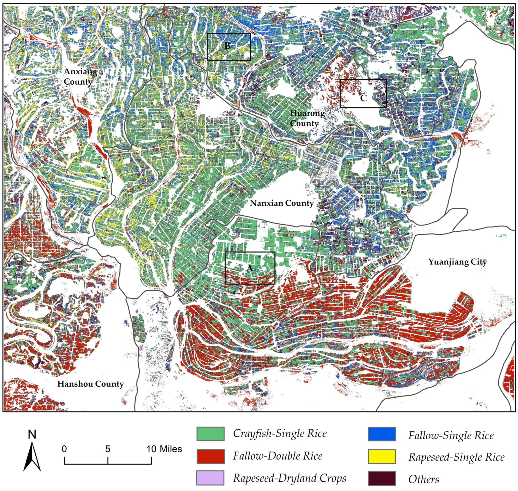
Overall, crop rotation distribution exhibited clear regional patterns (Figure 5). For instance, the southern parts of the study area were dominated by fallow-double rice rotation type, mostly in Hanshou county and Yuanjiang City. Crayfish-single rice was the dominant rotation type with a relatively clear and square border for every single field, especially in Huarong and Nanxian. In the eastern, northeastern, and northern regions, there were mostly fallow-single rice regions. In the northwestern part of the study area where sparsely distributed hills stand, mostly in western Nanxian County and Anxiang County, there is a higher proportion of rapeseed-single rice rotation type. Only a few smallholders cultivated dryland crops (rapeseed-dryland crops) due to limited access to water in the sloped fields of the hilly areas. We should also take note that there were still large, locally fragmented rotation patterns, showing typical characteristics of smallholders in Southern China.
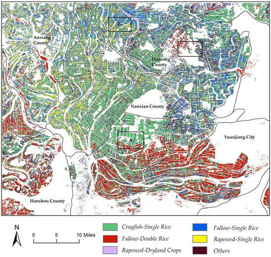
Figure 5.
Crop rotation classification in the study area. The white background indicates non-croplands.
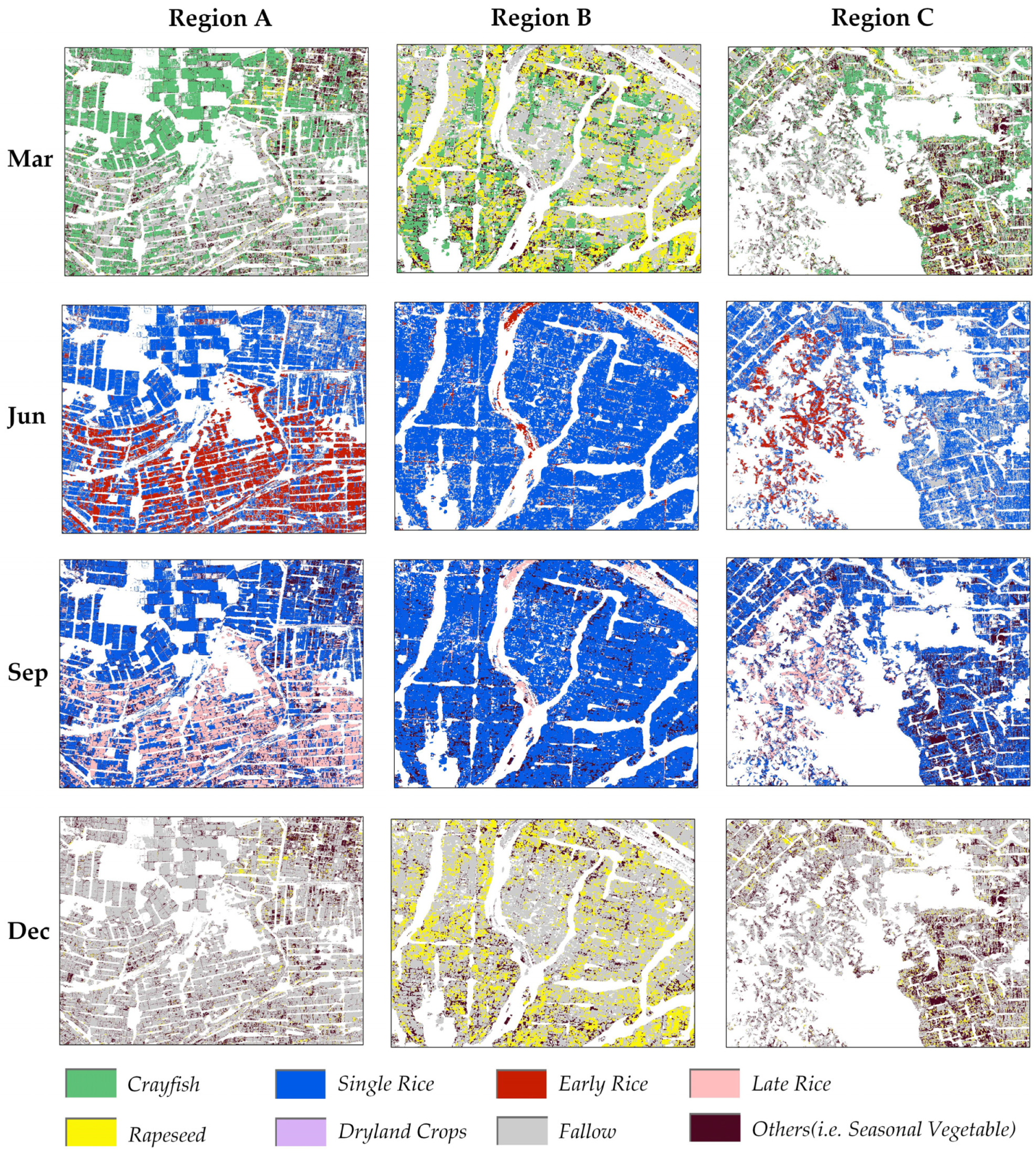
Local details of cross-seasonal changes of different crop types in selected regions were displayed in Figure 6. In March, rapeseed gradually entered the flowering period and farmers prepared to breed crayfish. By May, single rice and dryland crops were sowed. By June, early rice was about to ripen. Late rice was transplanted in late July. Dryland crops, single and late rice experienced their critical phenological stages during September. Only rapeseed and vegetables appeared in winter, and the majority of the fields were fallow.
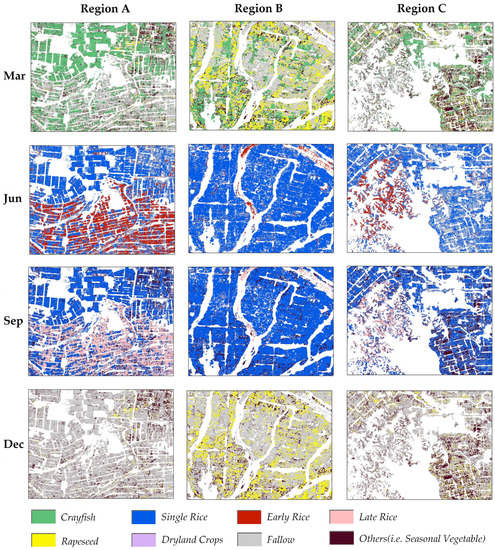
Figure 6.
Local details of cross-seasonal changes of crop types in selected regions mentioned in Figure 5.
Among all types, crayfish-single rice was a special rotation type in the study area, which was driven by business interests taking full advantage of fallow fields. The proportion of fallow-single rice was slightly higher than that of fallow-double rice due to less labor and administrative costs. Fallow-double rice was an intensive rotation system with a twice-planting practice (early rice and late rice) over a relatively short period. As stated by local farmers, smallholders preferred to grow single rice, as the total yield of single rice could be close to that of double rice due to advances in cultivar and farming practices. Winter–summer rotation systems (rapeseed-single rice and rapeseed-dryland crops) also altered crop types twice a year to obtain additional sources of income. Other rotation types, mainly for seasonal vegetables, had a short growing cycle and rapid change due to the diversity of the smallholder’s own needs.
6. Discussion
6.1. Evaluation of End-To-End Crop Rotation Mapping
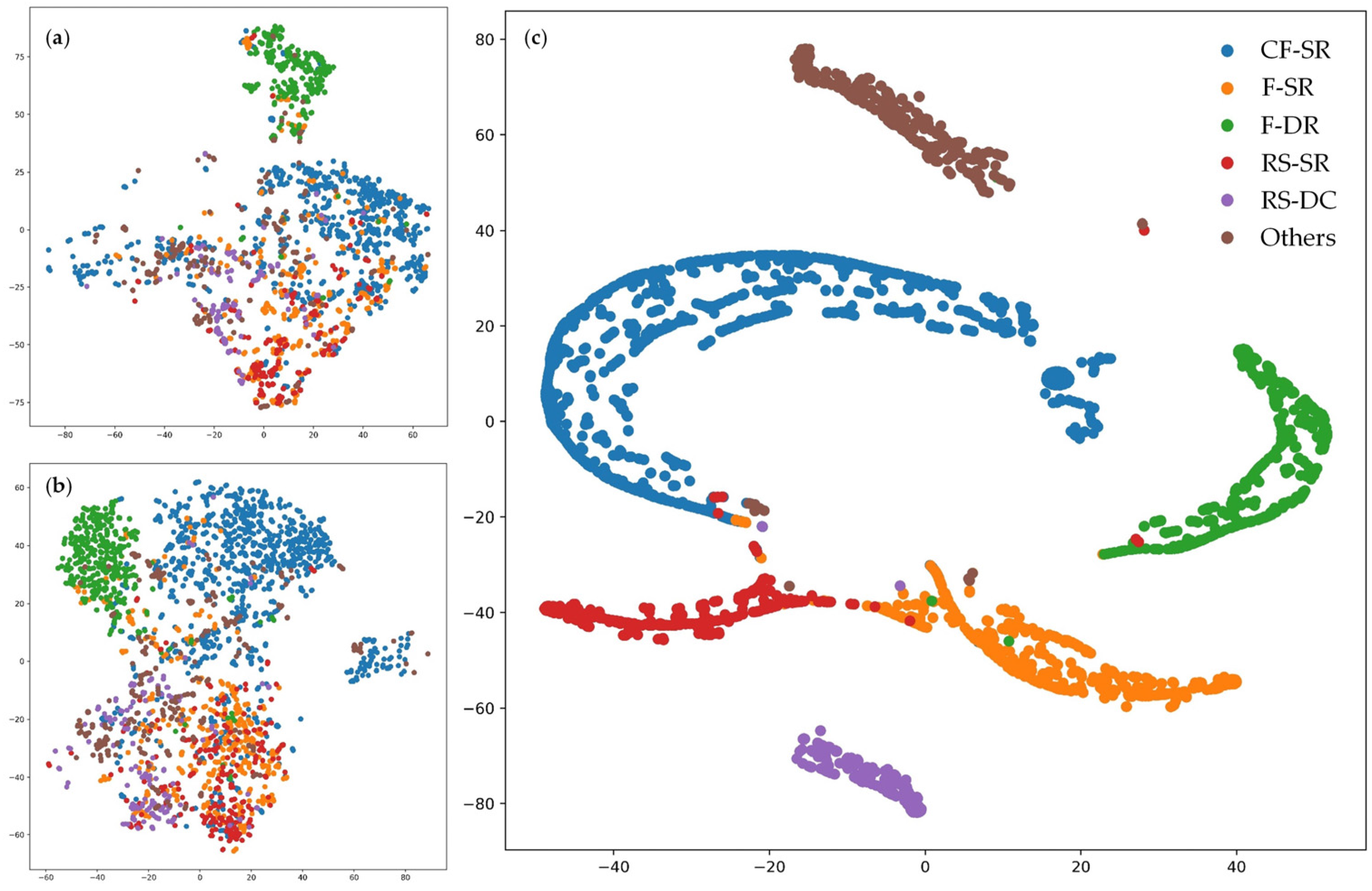
Our primary goal was to map practiced crop rotations using the SITS. The proposed model provided us the opportunity to generate high-resolution, intra-annual crop rotation information at regional scales, giving us insight into the distribution and seasonal changes of each crop type and supporting the subsequent agro-ecosystem analysis and application. Compared to the orginal satellite image time series, our model showed good separability among different rotation types visualized by the t-SNE statistical method (Figure 7). It further demonstrated the feasibility of extracting abundant crop rotation information hidden in the original time series without mapping and linking individual monoculture crop distribution or utilizing absolute phenological thresholds to segment different crop types [8,10].
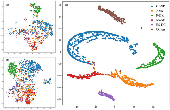
Figure 7.
Feature space based on t-SNE statistical method. (a) and (b) original NDVI and SAR time series; and (c) the last hidden layer in CRM.
We also tested the performance of Conv2D in our mission with an experiment retaining the framework of CRM while replacing all Conv1D with 2D. In the experiment, the CRM structure with Conv1D showed slightly better performance than Conv2D irrespective of the input vegetation indices that resulted from the fragmented land parcels in our study area. Compared to the effectiveness of Conv1D to extract robust temporal features and cross-seasonal dynamic changes from temporal profiles, Conv2D introduces more noise by cutting small patches of the input 2D samples to learn spatial information with the disturbance of fragmented fields.
To the best of our knowledge, this is the first study to map crop rotation systems in the study area. When considering the paddy rice cultivation system, our classification results were highly consistent with prior works [48,49,50,51], demonstrating the reliability of our model to a certain extent. Additionally, in contrast to previous works focusing on a single crop mapping, this proposed model was qualified to identify another two main types (fallow-single rice and crayfish-single rice) in the study area, emphasizing the fallow state in the rotation system and the symbiotic farming practice of crayfish and crops, which is new to the existing knowledge [30,51,52]. Thus, our rotation map not only provides a distribution of a local, general agricultural system but also provides multi-seasonal and multi-crop distribution maps if the data are divided into different points of time (Figure 5 and Figure 6). Such a model can be readily extended to help the agricultural department to monitor phenology, crop conditions, and agricultural practices, especially in the southern parts of China [53].
6.2. Necessity of Establishing the Dual-Stream Model for Multi-Source Data
Our model demonstrated that the performance of mapping rotation could be improved by leveraging a multi-source time series with the help of an attention mechanism. Among traditional data fusion methods, pixel-level fusion was impractical in this study due to the large discrepancy in data modality of multi-sensors that operate on different fundamental physical principles [54]. In addition, decision-level confusion was not the optimal option. It only combines the processed outputs derived by each data source in the last step, which cannot fully utilize the complementary and synergetic advantages of two sensors in the temporal domain [55]. Our results showed that the dual-stream model could exploit the interplay between the S1 and S2 time series by the adaptative concatenation operation, which proved highly significant for crop rotation mapping. For instance, CRM always outperformed CRM(S2), the model with only one single processing stream in all kinds of rotation types, especially for the easily confused rapeseed-single rice, fallow-single rice, and crayfish-single rice types. This also suggests the need to design a more sophisticated model to learn the synergy between the spatial and temporal dependencies in the two data sources. Previous studies also demonstrated that synergizing SAR and optical data in the deep learning model yielded the potential to learn the complementary information from two sensors even when the optical data had a long data gap [55]. As for the field of land cover classification, the capability of the dual-stream model has also been tested with the increase in accuracy from 5 to 16 points when feeding stacked Sentinel-1 and Sentinel-2 imagery into the classifier [36]. These findings are consistent with our results, which also proves the feasibility and necessity of processing multi-source temporal data. However, the approaches mentioned above did not take the diversity of each timestamp into account and treated them as the same. In our model, we addressed this issue by applying the attention mechanism to allocate reasonable weights according to the importance of each timestamp. This technique was shown to improve model accuracy, which was neglected in prior works [36].
7. Conclusions
This study proposed a hybrid deep learning architecture, namely CRM, to exploit radar and optical time series in the context of crop rotation mapping. Unlike most studies, the model was designed to leverage the complementary signals provided by different sensors and take advantage of popular deep learning frameworks to obtain complex intra-annual rotation information. The model we proposed is suitable for a complex planting system, lacking a uniform or specific key phenological state due to the diversity of crop types and flexibility of farming practice. This end-to-end architecture included a dedicated stream for each data source. Each stream was conducted by two deep learning blocks, a CNN and an attentive LSTM, taking both rotation features and contexture information into account. The final result was derived by concatenating the features learned by each source.
The experimental results demonstrated that the predicted images had reasonable accuracies (i.e., accuracy > 0.85) in mapping crop rotation, also showing how our proposed method outperformed other state-of-the-art, non-deep or deep learning solutions. Moreover, CRM was effective when extracting crop rotation features with the help of the deep synergy of SAR-optical time-series data and the attention mechanism, as our model showed a gain in overall accuracy of four points compared with ablation models such as CRM(S2) and CRM(NoAtt). However, we should point out that rotation types with short growth cycles, such as seasonal vegetables, can not be further subdivided due to the insufficient ability to capture the rapidly changing phenology. As cross-seasonal rotation maps contain rich dynamic information, it may be valuable to generate crop rotation layers instead of the static cropland data layers. To achieve such a goal, further exploration is required to extend the proposed architecture, not only in the temporal domain but also by considering and combining spatial or spectral information obtained from time-series satellite data.
Author Contributions
Conceptualization, Y.L., T.Y. and W.Z.; methodology, Y.L. and W.Z.; data curation, Y.L. and S.C.; writing—original draft preparation, Y.L. and T.Y.; writing—review and editing, T.Y. and W.Z.; visualization, Y.L. and S.C. All authors have read and agreed to the published version of the manuscript.
Funding
This research was funded by the National Natural Science Foundation of China, grant number NSFC 42171075.
Institutional Review Board Statement
Not applicable.
Informed Consent Statement
Not applicable.
Data Availability Statement
All data and model presented in this study are available on request from the corresponding author for research purpose.
Conflicts of Interest
The authors declare no conflict of interest.
References
- Panigrahy, S.; Sharma, S.A. Mapping of Crop Rotation Using Multidate Indian Remote Sensing Satellite Digital Data. ISPRS J. Photogramm. Remote Sens. 1997, 52, 85–91. [Google Scholar] [CrossRef]
- Zhao, J.; Yang, Y.; Zhang, K.; Jeong, J.; Zeng, Z.; Zang, H. Does Crop Rotation Yield More in China? A Meta-Analysis. Field Crop. Res. 2020, 245, 107659. [Google Scholar] [CrossRef]
- Wenbin, W.; Yu, Q.; You, L.; Chen, K.; Tang, H.; Liu, J. Global Cropping Intensity Gaps: Increasing Food Production without Cropland Expansion. Land Use Policy 2018, 76, 515–525. [Google Scholar] [CrossRef]
- Barbieri, P.; Pellerin, S.; Seufert, V.; Nesme, T. Changes in Crop Rotations Would Impact Food Production in an Organically Farmed World. Nat. Sustain. 2019, 2, 378–385. [Google Scholar] [CrossRef]
- Kuenzer, C.; Knauer, K. Remote Sensing of Rice Crop Areas. Int. J. Remote Sens. 2013, 34, 2101–2139. [Google Scholar] [CrossRef]
- Merlos, F.A.; Hijmans, R.J. The Scale Dependency of Spatial Crop Species Diversity and Its Relation to Temporal Diversity. Proc. Natl. Acad. Sci. USA 2020, 117, 26176–26182. [Google Scholar] [CrossRef] [PubMed]
- Konduri, V.S.; Kumar, J.; Hargrove, W.W.; Hoffman, F.M.; Ganguly, A.R. Mapping Crops within the Growing Season across the United States. Remote Sens. Environ. 2020, 251, 112048. [Google Scholar] [CrossRef]
- Multi-Data Approach for remote sensing-based regional crop rotation mapping: A case study for the Rur catchment, Germany. Int. J. Appl. Earth Obs. Geoinf. 2017, 61, 55–69. [CrossRef]
- Han, J.; Zhang, Z.; Luo, Y.; Cao, J.; Zhang, L.; Zhang, J.; Li, Z. The RapeseedMap10 Database: Annual Maps of Rapeseed at a Spatial Resolution of 10 m Based on Multi-Source Data. Earth Syst. Sci. Data 2021, 13, 2857–2874. [Google Scholar] [CrossRef]
- Chen, Y.; Lu, D.; Moran, E.; Batistella, M.; Dutra, L.V.; Sanches, I.D.; da Silva, R.F.B.; Huang, J.; Luiz, A.J.B.; de Oliveira, M.A.F. Mapping Croplands, Cropping Patterns, and Crop Types Using MODIS Time-Series Data. Int. J. Appl. Earth Obs. Geoinf. 2018, 69, 133–147. [Google Scholar] [CrossRef]
- Li, R.; Xu, M.; Chen, Z.; Gao, B.; Cai, J.; Shen, F.; He, X.; Zhuang, Y.; Chen, D. Phenology-Based Classification of Crop Species and Rotation Types Using Fused MODIS and Landsat Data: The Comparison of a Random-Forest-Based Model and a Decision-Rule-Based Model. Soil Tillage Res. 2021, 206, 104838. [Google Scholar] [CrossRef]
- Wang, S.; Azzari, G.; Lobell, D.B. Crop Type Mapping without Field-Level Labels: Random Forest Transfer and Unsupervised Clustering Techniques. Remote Sens. Environ. 2019, 222, 303–317. [Google Scholar] [CrossRef]
- Zhong, L.; Hawkins, T.; Biging, G.; Gong, P. A Phenology-Based Approach to Map Crop Types in the San Joaquin Valley, California. Int. J. Remote Sens. 2011, 32, 7777–7804. [Google Scholar] [CrossRef]
- Liu, J.; Li, L.; Huang, X.; Liu, Y.; Li, T. Mapping Paddy Rice in Jiangsu Province, China, Based on Phenological Parameters and a Decision Tree Model. Front. Earth Sci. 2019, 13, 111–123. [Google Scholar] [CrossRef]
- Deschamps, B.; McNairn, H.; Shang, J.; Jiao, X. Towards Operational Radar-Only Crop Type Classification: Comparison of a Traditional Decision Tree with a Random Forest Classifier. Can. J. Remote Sens. 2012, 38, 60–68. [Google Scholar] [CrossRef]
- Yang, N.; Liu, D.; Feng, Q.; Xiong, Q.; Zhang, L.; Ren, T.; Zhao, Y.; Zhu, D.; Huang, J. Large-Scale Crop Mapping Based on Machine Learning and Parallel Computation with Grids. Remote Sens. 2019, 11, 1500. [Google Scholar] [CrossRef] [Green Version]
- Hao, P.; Zhan, Y.; Wang, L.; Niu, Z.; Shakir, M. Feature Selection of Time Series MODIS Data for Early Crop Classification Using Random Forest: A Case Study in Kansas, USA. Remote Sens. 2015, 7, 5347–5369. [Google Scholar] [CrossRef] [Green Version]
- Zheng, B.; Myint, S.W.; Thenkabail, P.S.; Aggarwal, R.M. A Support Vector Machine to Identify Irrigated Crop Types Using Time-Series Landsat NDVI Data. Int. J. Appl. Earth Obs. Geoinf. 2015, 34, 103–112. [Google Scholar] [CrossRef]
- You, N.; Dong, J.; Huang, J.; Du, G.; Zhang, G.; He, Y.; Yang, T.; Di, Y.; Xiao, X. The 10-m Crop Type Maps in Northeast China during 2017–2019. Sci. Data 2021, 8, 41. [Google Scholar] [CrossRef]
- Peña, J.M.; Gutiérrez, P.A.; Hervás-Martínez, C.; Six, J.; Plant, R.E.; López-Granados, F. Object-Based Image Classification of Summer Crops with Machine Learning Methods. Remote Sens. 2014, 6, 5019–5041. [Google Scholar] [CrossRef] [Green Version]
- Pan, Y.; Li, L.; Zhang, J.; Liang, S.; Zhu, X.; Sulla-Menashe, D. Winter Wheat Area Estimation from MODIS-EVI Time Series Data Using the Crop Proportion Phenology Index. Remote Sens. Environ. 2012, 119, 232–242. [Google Scholar] [CrossRef]
- Guan, X.; Huang, C.; Liu, G.; Meng, X.; Liu, Q. Mapping Rice Cropping Systems in Vietnam Using an NDVI-Based Time-Series Similarity Measurement Based on DTW Distance. Remote Sens. 2016, 8, 19. [Google Scholar] [CrossRef] [Green Version]
- Csillik, O.; Belgiu, M.; Asner, G.P.; Kelly, M. Object-Based Time-Constrained Dynamic Time Warping Classification of Crops Using Sentinel-2. Remote Sens. 2019, 11, 1257. [Google Scholar] [CrossRef] [Green Version]
- Maus, V.; Câmara, G.; Cartaxo, R.; Sanchez, A.; Ramos, F.M.; de Queiroz, G.R. A Time-Weighted Dynamic Time Warping Method for Land-Use and Land-Cover Mapping. IEEE J. Sel. Top. Appl. Earth Obs. Remote Sens. 2016, 9, 3729–3739. [Google Scholar] [CrossRef]
- LeCun, Y.; Bengio, Y.; Hinton, G. Deep Learning. Nature 2015, 521, 436–444. [Google Scholar] [CrossRef]
- Sun, Z.; Di, L.; Fang, H.; Burgess, A. Deep Learning Classification for Crop Types in North Dakota. IEEE J. Sel. Top. Appl. Earth Obs. Remote Sens. 2020, 13, 2200–2213. [Google Scholar] [CrossRef]
- Yang, S.; Gu, L.; Li, X.; Jiang, T.; Ren, R. Crop Classification Method Based on Optimal Feature Selection and Hybrid CNN-RF Networks for Multi-Temporal Remote Sensing Imagery. Remote Sens. 2020, 12, 3119. [Google Scholar] [CrossRef]
- Zhong, L.; Hu, L.; Zhou, H. Deep Learning Based Multi-Temporal Crop Classification. Remote Sens. Environ. 2019, 221, 430–443. [Google Scholar] [CrossRef]
- Crisóstomo de Castro Filho, H.; Abílio de Carvalho Júnior, O.; Ferreira de Carvalho, O.L.; Pozzobon de Bem, P.; dos Santos de Moura, R.; Olino de Albuquerque, A.; Rosa Silva, C.; Guimarães Ferreira, P.H.; Fontes Guimarães, R.; Trancoso Gomes, R.A. Rice Crop Detection Using LSTM, Bi-LSTM, and Machine Learning Models from Sentinel-1 Time Series. Remote Sens. 2020, 12, 2655. [Google Scholar] [CrossRef]
- Sun, Z.; Di, L.; Fang, H. Using Long Short-Term Memory Recurrent Neural Network in Land Cover Classification on Landsat and Cropland Data Layer Time Series. Int. J. Remote Sens. 2019, 40, 593–614. [Google Scholar] [CrossRef]
- Rußwurm, M.; Körner, M. Temporal Vegetation Modelling Using Long Short-Term Memory Networks for Crop Identification from Medium-Resolution Multi-Spectral Satellite Images. In Proceedings of the 2017 IEEE Conference on Computer Vision and Pattern Recognition Workshops (CVPRW), Honolulu, Hawaii, 21–26 July 2017; pp. 1496–1504. [Google Scholar]
- Cué La Rosa, L.E.; Queiroz Feitosa, R.; Nigri Happ, P.; Del’Arco Sanches, I.; Ostwald Pedro da Costa, G.A. Combining Deep Learning and Prior Knowledge for Crop Mapping in Tropical Regions from Multitemporal SAR Image Sequences. Remote Sens. 2019, 11, 2029. [Google Scholar] [CrossRef] [Green Version]
- Wei, S.; Zhang, H.; Wang, C.; Wang, Y.; Xu, L. Multi-Temporal SAR Data Large-Scale Crop Mapping Based on U-Net Model. Remote Sens. 2019, 11, 68. [Google Scholar] [CrossRef] [Green Version]
- Adrian, J.; Sagan, V.; Maimaitijiang, M. Sentinel SAR-Optical Fusion for Crop Type Mapping Using Deep Learning and Google Earth Engine. ISPRS J. Photogramm. Remote Sens. 2021, 175, 215–235. [Google Scholar] [CrossRef]
- Liao, C.; Wang, J.; Xie, Q.; Baz, A.A.; Huang, X.; Shang, J.; He, Y. Synergistic Use of Multi-Temporal RADARSAT-2 and VENµS Data for Crop Classification Based on 1D Convolutional Neural Network. Remote Sens. 2020, 12, 832. [Google Scholar] [CrossRef] [Green Version]
- Ienco, D.; Interdonato, R.; Gaetano, R.; Ho Tong Minh, D. Combining Sentinel-1 and Sentinel-2 Satellite Image Time Series for Land Cover Mapping via a Multi-Source Deep Learning Architecture. ISPRS J. Photogramm. Remote Sens. 2019, 158, 11–22. [Google Scholar] [CrossRef]
- Mou, L.; Bruzzone, L.; Zhu, X.X. Learning Spectral-Spatial-Temporal Features via a Recurrent Convolutional Neural Network for Change Detection in Multispectral Imagery. IEEE Trans. Geosci. Remote Sens. 2019, 57, 924–935. [Google Scholar] [CrossRef] [Green Version]
- Rawat, A.; Kumar, A.; Upadhyay, P.; Kumar, S. Deep Learning-Based Models for Temporal Satellite Data Processing: Classification of Paddy Transplanted Fields. Ecol. Inform. 2021, 61, 101214. [Google Scholar] [CrossRef]
- Li, C.; Li, H.; Li, J.; Lei, Y.; Li, C.; Manevski, K.; Shen, Y. Using NDVI Percentiles to Monitor Real-Time Crop Growth. Comput. Electron. Agric. 2019, 162, 357–363. [Google Scholar] [CrossRef]
- Camps-Valls, G.; Campos-Taberner, M.; Moreno-Martínez, Á.; Walther, S.; Duveiller, G.; Cescatti, A.; Mahecha, M.D.; Muñoz-Marí, J.; García-Haro, F.J.; Guanter, L.; et al. A Unified Vegetation Index for Quantifying the Terrestrial Biosphere. Sci. Adv. 2021, 7, eabc7447. [Google Scholar] [CrossRef] [PubMed]
- Srivastava, N.; Hinton, G.; Krizhevsky, A.; Sutskever, I.; Salakhutdinov, R. Dropout: A Simple Way to Prevent Neural Networks from Overfitting. J. Mach. Learn. Res. 2014, 15, 1929–1958. [Google Scholar]
- Zhou, Y.; Luo, J.; Feng, L.; Yang, Y.; Chen, Y.; Wu, W. Long-Short-Term-Memory-Based Crop Classification Using High-Resolution Optical Images and Multi-Temporal SAR Data. GIScience Remote Sens. 2019, 56, 1170–1191. [Google Scholar] [CrossRef]
- Britz, D.; Guan, M.Y.; Luong, M.-T. Efficient Attention Using a Fixed-Size Memory Representation. arXiv 2017, arXiv:1707.00110. [Google Scholar]
- Tatsumi, K.; Yamashiki, Y.; Canales Torres, M.A.; Taipe, C.L.R. Crop Classification of Upland Fields Using Random Forest of Time-Series Landsat 7 ETM+ Data. Comput. Electron. Agric. 2015, 115, 171–179. [Google Scholar] [CrossRef]
- He, T.; Xie, C.; Liu, Q.; Guan, S.; Liu, G. Evaluation and Comparison of Random Forest and A-LSTM Networks for Large-Scale Winter Wheat Identification. Remote Sens. 2019, 11, 1665. [Google Scholar] [CrossRef] [Green Version]
- Qiu, C.; Mou, L.; Schmitt, M.; Zhu, X.X. Local Climate Zone-Based Urban Land Cover Classification from Multi-Seasonal Sentinel-2 Images with a Recurrent Residual Network. ISPRS J. Photogramm. Remote Sens. 2019, 154, 151–162. [Google Scholar] [CrossRef]
- Kingma, D.P.; Ba, J. Adam: A Method for Stochastic Optimization. arXiv 2017, arXiv:1412.6980. [Google Scholar]
- Zhang, M.; Lin, H.; Wang, G.; Sun, H.; Fu, J. Mapping Paddy Rice Using a Convolutional Neural Network (CNN) with Landsat 8 Datasets in the Dongting Lake Area, China. Remote Sens. 2018, 10, 1840. [Google Scholar] [CrossRef] [Green Version]
- Zhang, X.; Wu, B.; Ponce-Campos, G.E.; Zhang, M.; Chang, S.; Tian, F. Mapping Up-to-Date Paddy Rice Extent at 10 M Resolution in China through the Integration of Optical and Synthetic Aperture Radar Images. Remote Sens. 2018, 10, 1200. [Google Scholar] [CrossRef] [Green Version]
- Cai, Y.; Lin, H.; Zhang, M. Mapping Paddy Rice by the Object-Based Random Forest Method Using Time Series Sentinel-1/Sentinel-2 Data. Adv. Space Res. 2019, 64, 2233–2244. [Google Scholar] [CrossRef]
- Xiao, X.; Boles, S.; Liu, J.; Zhuang, D.; Frolking, S.; Li, C.; Salas, W.; Moore, B. Mapping Paddy Rice Agriculture in Southern China Using Multi-Temporal MODIS Images. Remote Sens. Environ. 2005, 95, 480–492. [Google Scholar] [CrossRef]
- Dong, J.; Xiao, X.; Menarguez, M.A.; Zhang, G.; Qin, Y.; Thau, D.; Biradar, C.; Moore, B. Mapping Paddy Rice Planting Area in Northeastern Asia with Landsat 8 Images, Phenology-Based Algorithm and Google Earth Engine. Remote Sens. Environ. 2016, 185, 142–154. [Google Scholar] [CrossRef] [Green Version]
- Ye, Q.; Yang, X.; Dai, S.; Chen, G.; Li, Y.; Zhang, C. Effects of Climate Change on Suitable Rice Cropping Areas, Cropping Systems and Crop Water Requirements in Southern China. Agric. Water Manag 2015, 159, 35–44. [Google Scholar] [CrossRef]
- Joshi, N.; Baumann, M.; Ehammer, A.; Fensholt, R.; Grogan, K.; Hostert, P.; Jepsen, M.R.; Kuemmerle, T.; Meyfroidt, P.; Mitchard, E.T.A.; et al. A Review of the Application of Optical and Radar Remote Sensing Data Fusion to Land Use Mapping and Monitoring. Remote Sens. 2016, 8, 70. [Google Scholar] [CrossRef] [Green Version]
- Zhao, W.; Qu, Y.; Chen, J.; Yuan, Z. Deeply Synergistic Optical and SAR Time Series for Crop Dynamic Monitoring. Remote Sens. Environ. 2020, 247, 111952. [Google Scholar] [CrossRef]
Publisher’s Note: MDPI stays neutral with regard to jurisdictional claims in published maps and institutional affiliations. |
© 2021 by the authors. Licensee MDPI, Basel, Switzerland. This article is an open access article distributed under the terms and conditions of the Creative Commons Attribution (CC BY) license (https://creativecommons.org/licenses/by/4.0/).

