Within-Field Yield Prediction in Cereal Crops Using LiDAR-Derived Topographic Attributes with Geographically Weighted Regression Models

Abstract

Accurate yield estimation and optimized agricultural management is a key goal in precision agriculture, while depending on many different production attributes, such as soil properties, fertilizer and irrigation management, the weather, and topography.The need for timely and accurate sensing of these inputs at the within field-scale has led to increased adoption of very high-resolution remote and proximal sensing technologies. With regard to topography attributes, greater attention is currently being devoted to LiDAR datasets (Light Detection and Ranging), mainly because numerous topographic variables can be derived at very high spatial resolution from these datasets. The current study uses LiDAR elevation data from agricultural land in southern Ontario, Canada to derive several topographic attributes such as slope, and topographic wetness index, which were then correlated to seven years of crop yield data. The effectiveness of each topographic derivative was independently tested using a moving-window correlation technique. Finally, the correlated derivatives were selected as explanatory variables for geographically weighted regression (GWR) models. The global coefficient of determination values (determined from an average of all the local relationships) were found to be R² = 0.80 for corn, R² = 0.73 for wheat, R² = 0.71 for soybeans and R² = 0.75 for the average of all crops. These results indicate that GWR models using topographic variables derived from LiDAR can effectively explain yield variation of several crop types on an entire-field scale.

1. Introduction

Precision agriculture technologies are increasingly dependent on accurate crop yield information in order to be effective. Unfortunately, not all farmers are able to collect these data due to the initial cost or because of the technological knowledge required to extract and examine the data. This is especially true in developing regions where the use of yield-monitoring technology is rare. In addition, data protection and privacy rights can also make it difficult to access annual yield data [1]. In these cases, it would be beneficial to use proxies for crop yield that can be easily determined without the need for yield-monitoring technology that require more investment and time.

Topographic variables have been shown to have significant influence on crop yield, most likely due to surficial hydrological processes related to local topographic variation [2,3,4]. For instance, soil water, nutrients such as nitrogen and phosphorous, and organic matter are all essential in the development of agricultural crops and much of their spatial distribution can be explained with the use of surficial topographic variables [5,6,7,8,9]. Therefore, using topographic attributes may be a viable method for measuring within-field crop yield variability to identify low-yielding regions of cropland where ecologically beneficial land uses may be more suitable [10]. This would allow for field assessment without the need for crop yield data and may potentially increase the amount of lands set aside for ecological or environmental benefits [10]. This approach may also provide supplemental insight into crop yield potential in fields that have sparsely collected crop yield data.

Topographic variability is one of the main controls on surface flow and is subsequently one of the most studied flow-inducing gradients for water and nutrients [11,12,13]. Leveraging the potential energy provided by gravity and vertical displacement, topographic variability influences hydrological processes such as overland flow and throughflow, therefore affecting the distribution of soil water [12]. This is easily observed in regions with high topographic variability, as water tends to pool in lower-lying areas while elevated areas are subject to drier conditions. Surface characteristics that dictate crop yield potential, such as surface moisture and available nutrients, often follow the spatial distribution represented by these topographic attributes. Therefore, including a variety of these attributes when assessing the relationships between topography and yield should be essential [2]. For example, Green et al. [2] showed that slope, elevation and Wetness Index have significant explanatory control on crop yield with the use of neural network and multiple linear regression models. Heil et al. (Ref. [5] experimented with the use of topographic parameters to predict grain yields, notably concluding that catchment area, valley depth, plan curvature, profile curvature and convergence are significant predictors of crop yields. Varying results between studies highlight the necessity to include a variety of topographic parameters as model inputs when predicting crop yield based on local topography. Attribute raster spatial resolution may also impact the viability of specific topographic attributes [12,14].

Aerial-based LiDAR systems and GPS (Global Positioning System) technologies have also made it efficient and reasonably cost-effective to collect highly accurate surficial data for large areas [7,15]. This has led to extensive use LiDAR-generated digital elevation models (DEM) in agricultural regions, where governments, research groups and private entities have collected precise elevation data. In addition to the recent developments made in surface data collection technology and expanded DEM coverage, the methods used to evaluate land surfaces are continually developed as well. LiDAR derived topographic attributes developed from surface data can be used to explain the distribution of surface water and nutrients, therefore indicating areas where an increase in potential crop yield can be achieved.

One of the benefits of these expanding datasets is the opportunity to assess topography-controlled yield potential of farms where yield data do not exist or is inaccessible. This opportunity will continue to grow as the geographic coverage of DEMs expands and may contribute to the ability to assess potential within field yield variations in remote locations or in developing regions. The use of these techniques may be economically beneficial to agricultural practitioners, while providing information to encourage the implementation of ecosystem service-providing land uses [10].

This study aims to assess how topographic attributes created from fine-resolution LiDAR surface data can be used to evaluate in-field crop yield variation and assess relative yield variability within an agricultural field in southern Ontario, Canada. This was accomplished through two main objectives: (1) Assess which topographic attributes are most effective for predicting crop yield variance and for which crop types; and (2) use a geographically weighted regression technique to determine the extent to which topographic derivates can predict in-field crop yield variation and to identify local areas of topographically restricted yield potential that may be better suited for other land uses.

2. Study Area and Methods

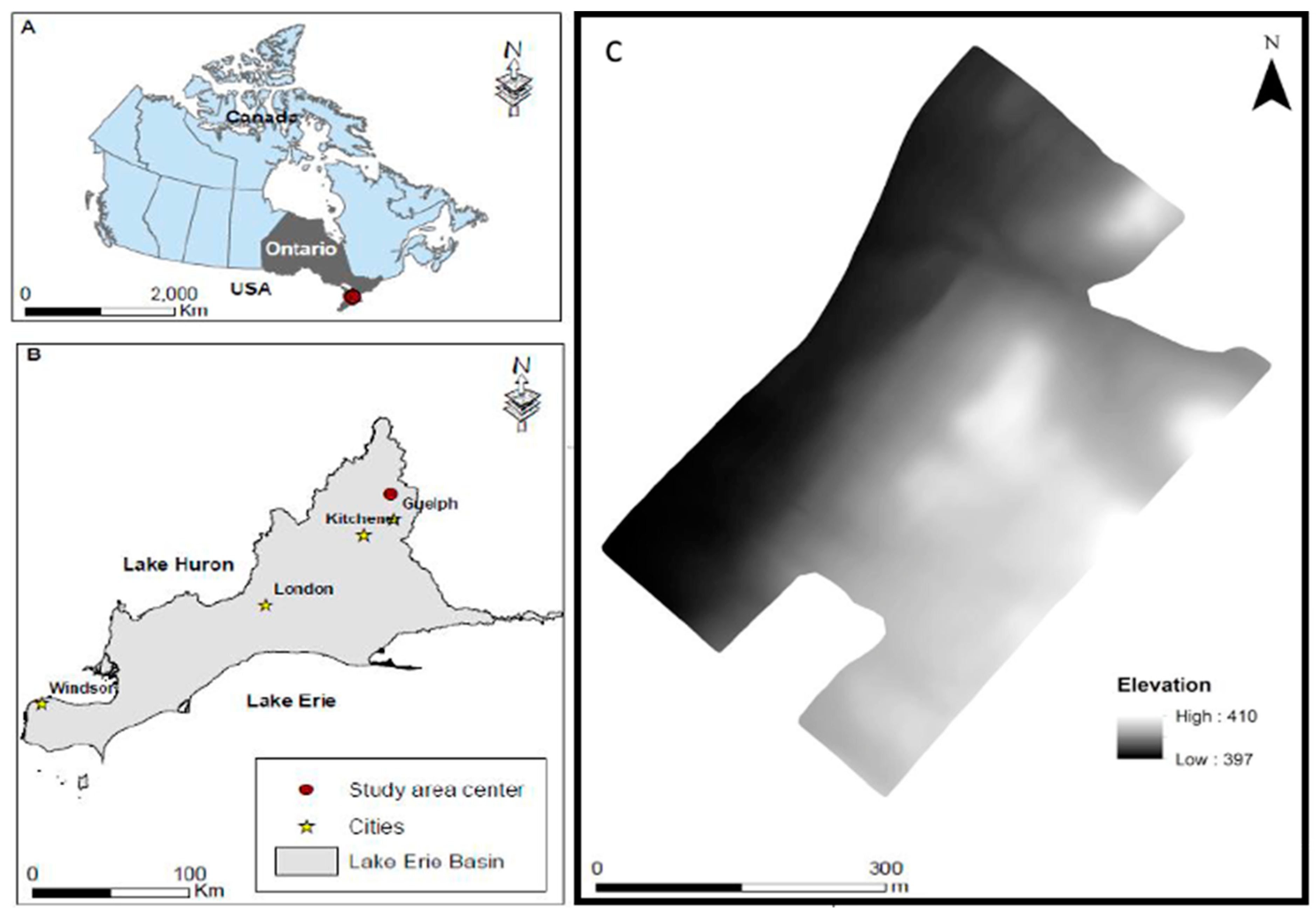
2.1. Site Description

This research was conducted in an agricultural field located within the Canadian Lake Erie basin of southwestern Ontario, Canada (Figure 1A,B). Southwestern Ontario has regions of highly active agricultural activity, including more than 1.2 million hectares of annually harvested crop land [16]. The most commonly grown crops in this region include corn, soybeans, and winter wheat [16]. These crops are generally grown in crop rotations to promote the sustainability of the production system and soil health. Cover crops are widely adopted by farmers as a practice to protect fields from soil erosion and to promote organic matter accumulation within the field [17].

The study field covers approximately 26 hectares near the city of Guelph Ontario, Canada (Figure 1C). The soils are typical of the surrounding region, classified as Hillsburgh fine sandy loam series [18]. The site topography can be described as having irregular, lightly sloping terrains. An elevated ridge runs on a 40° orientation over the length of the field. The elevation of the field ranges from 397 m to 410 m above sea level (Figure 1C) with slopes ranging from 0° to 9°. There are several depressions throughout the field and a ephemeral creek runs along the north-west side of the field, with the topography sloping toward it.

The field is owned and managed by a private farming company and agricultural decisions are managed similarly to other farms in the surrounding area. Crops are subject to nutrient application as needed and are visually monitored by farm operators and their agronomy team throughout the growing season. Crops are generally planted using no-till practices with soy and wheat crops planted using an air seed drill and corn using a modern corn planter.

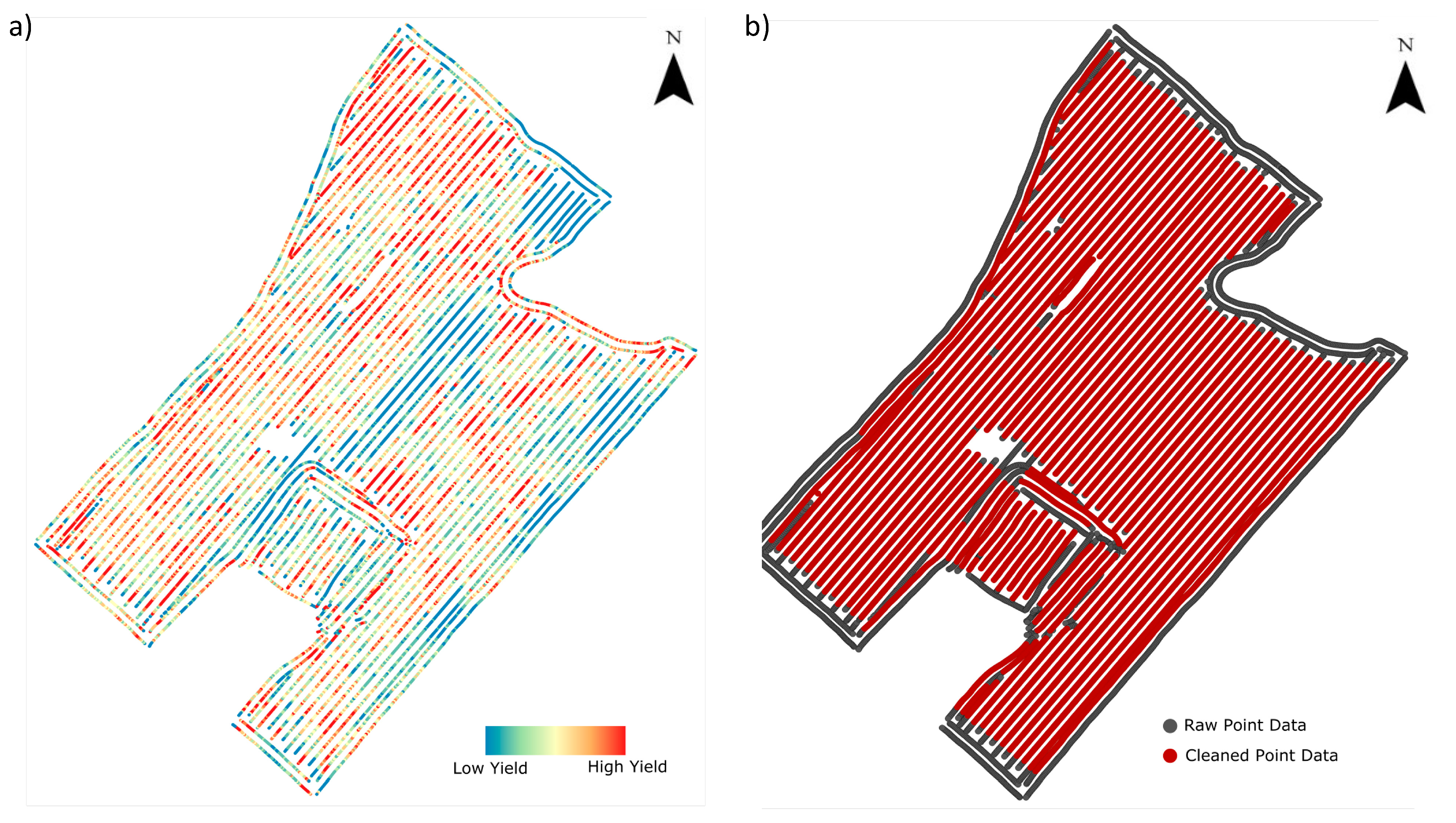
2.2. Processing Crop Yield Data

Crop yield data for this research were collected from the farmers that own and manage the study site’s farming operation. The yield data were collected for 2011–2018, as shown in

Table 1. Crop types included in this study.

Year	Crop
2011	Soybeans
2013	Soybeans
2014	Corn
2015	Soybeans
2016	Winter Wheat
2017	Soybeans
2018	Corn

. A commercial crop yield monitor, mounted to a traditional combine harvester, was used to measure yield. The device measures the amount of flowing grain passed through the elevator of the combine during harvest and then tags each measurement with real-time GPS coordinates. A point containing a yield measurement is created every second, generating a dense network of points that cover the field. The data are collected and formatted as georeferenced points (i.e., shapefiles) that were viewed and manipulated in a geographic information system (GIS).

Following [20], the crop yield data were cleaned to remove incorrect values recorded by the yield monitor. Commercial yield monitors are prone to erroneous data when harvested rows overlap, suggesting that there is a low yielding crop in specific areas of the field. Therefore, straight-line sequences of points that showed near-zero yield were removed from the dataset. Additionally, all points along the edge of the fields were removed to account for the head of the harvesting equipment potentially not being filled end-to-end during harvesting. This event is minimal through the interior of the field, but field edges are prone to being harvested without a full swath. When the combine begins harvesting each length of the field, there is also potential for the yield monitor to begin recording before flowing grain is measured. This results in the initial points of a row appearing to yield poorly. In these cases, points were removed from the dataset. An example image of the raw crop yields (before filtering) for an individual year (2017) is shown in Figure 2a. The points removed based on known areas potential yield estimation bias is shown in Figure 2b. Further description of crop yield for this field are presented in Capmourteres et al. [10].

The output yield shapefiles were interpolated to generate continuous raster surfaces for the entire field. The raster surfaces were created using a two-dimensional minimum curvature spline technique, implemented in ArcMap. This method was chosen because the method minimizes inflated curvature between points and ensures point data values are left intact within the raster cells [21]. Spline-generated raster surfaces are also typically smoother than raster surfaces produced by other interpolation techniques, which aids in visual interpretation of the results [22]. The spatial scale of the interpolated yield data was 0.5 m, this spatial scale was selected to match the spatial resolution of the topographic data (and its derivatives) as described in Section 2.3.

The newly created yield raster maps were normalized between 0 and 1 to allow for evenly weighted comparison between different crops using Equation (1). The yield at raster location x was normalized (x′) as:

$$x^{\prime }=\frac{x-Field Minimum}{Field Maximum-Field Minimum}$$

(1)

where the maximum and minimum values are highest and lowest yield observations on the field, following screening for anomalous values described above. This removes much of the inter-annual variance and the natural differences in yields by crop type. After normalization, the average of all yield rasters was also calculated to allow for spatial analyses on multiple years of crop yields. Averages for each crop were also calculated in this manner. The inclusion of multiple years of normalized yield data was completed to further minimize the effects that climate anomalies or agricultural management decisions may have had on resulting crop yields [15,23,24]. It must be noted that although there are benefits to this approach, it naturally excludes the ability to measure inter-annual factors on crop yield such as meteorological differences between years. Since there was only one year of wheat data available, the single layer represents wheat for the study.

2.3. LiDAR Dataset Acquisition and Processing

A LiDAR-derived DEM was created for the study site with the use of publicly available data collected by the Ontario Ministry of Food and Rural Affairs (OMAFRA) and the Ontario Ministry of Natural Resources and Forestry (MNRF). The LiDAR data were collected using a Leica geosystems ADS100 sensor from an airborne platform (2377 m AMT) over the studied field in 2017 and 2018 during the non-growing season, thus minimizing the number and effect of off terrain objects including vegetation canopies. The dataset used for this study was an interpolated 0.5 m bare-earth raster DEM derived from the LiDAR point clouds using a triangulation-based routine.

Topographic derivatives (shown in in

Table 2. Topographic attributes included in the regression analysis.

Topographic Attribute	Description	Source
Circular variance of aspect	Local slope aspect variance	[32]
Depression depth	Vertical depth of depressions	[33]
Downslope Index	Slope gradient between a cell and downslope cell	[34]
Catchment area with divergent flow (upslope area)	Multi-directional flow algorithm	[35]
Impoundment size index	Resulting upslope impoundment from placement of dam	[36]
Plan curvature	Curvature perpendicular to dominant slope angle	[37]
Profile curvature	Curvature parallel to dominant slope angle	[37]
Relative topographic position	Cell elevation relative to surrounding cells	[38]
Slope	Surface gradient	[37]
Tangential curvature	Plan curvature related to slope	[37]
Topographic wetness index	Steady state soil moisture index based slope contributing area	[39]
Total curvature	Curvature across a surface	[37]
Upslope flow path length	Average length of each cell’s upslope flow paths	[31]

) were selected based on pertinent theoretical and applied literature and raster layers created for each of the tested topographic derivatives [15,25,26,27,28]. For example, a crop’s dependence on soil water to produce a substantial yield makes layers associated with water movement appropriate for yield forecasting. Flow-driven nutrient movement may also indicate areas of higher yield potential [29]. Each layer was calculated using the DEM of the field and surrounding area in order to minimize potential unnatural edge-effects of the field boundary. Derivative raster layers were then clipped to match the extent of the field. The created topographic derivatives can be split into two subgroups: primary and secondary. Primary derivatives are those calculated directly from the DEM (i.e., slope, aspect), while secondary derivatives rely on a combination of primary surface derivatives or developed indices (i.e., topographic wetness index) to model topographic characteristics [30].

All the included variables and the source algorithms are briefly described in Table 2. Each of the source the algorithms were run using Whitebox-Tools [31]. Including a wide range of topographic derivatives can provide insight into which variables should be included in future models. This is critical for model transferability, as it may encourage the proper selection of variables to be chosen to fit the area of focus. It also allows for the topographic attributes to compensate for each other if there are distinct features within a field that influence crop yield variability.

2.4. Statistical Analysis

2.4.1. Field-Wide Statistical Analysis

In our first stage of analysis, a set of 13 topographic derivatives (Table 2) were individually correlated against crop yield variance to identify which attributes may be the most important factors for use in a multi-input regression. Linear regressions were performed between each topographic variable and average crop yield to assess their global (i.e., field-wide) relationships. Linear regressions were computed using R statistical analysis software [40].

2.4.2. Local Statistical Analysis

In addition to global or field average correlations, a moving-window technique [31,38] was used over the raster layers to calculate the Pearson correlation (i.e., r) coefficient. Then, the obtained r coefficients were used to observe local influence of the topographic attributes and to explain yield variance. To complete this step, the moving window tool collects cell values from each raster layer within a user-specified moving window and then performs Pearson’s correlation analysis on the selected values to calculate a single coefficient for each cell. For this study the chosen window size was 50 × 50 m to balance between sufficient sample size (number of samples greater than ~30) while minimizing the search distance. This window size was also chosen to strike a balance between the necessary sample size and scale of the terrain feature within the field and to form areas large enough for identification of management zones for future precision agricultural-based applications (which in this case would be limited the size of the field equipment). This technique allows for spatial influence from localized neighbouring cells that would otherwise be neglected from the analysis if the correlation were calculated in a global or point method [41,42].

2.4.3. Geographic Weighted Regression

In our second analysis, a geographic weighted regression (GWR) technique was used to evaluate the spatial relationship between tested topographic derivatives and crop yield. This method creates many linear regression models while incorporating geographic location into its analysis, enabling the model to assign location-based weight to attributes and compensate for variable non-stationarity [43]. The regression operates by surveying and considering data from neighbouring locations that can influence each individual output value. This allows the created model to consider local area in its analysis, similar to the moving-window technique described above for testing for individual correlation. This localized method of multiple regression has been shown to improve model accuracy, outperforming standard ordinary least squares methods, when input variables are considered nonstationary [41,43,44]. The approach also provides opportunities to observe where, within the agricultural field, each variable is contributing most to the output of the model. GWR models are naturally sensitive to collinearity between variables at global and local scales [43].

For this study, the GWR methodology was applied using ArcGIS. The algorithm selected uses the Akaike Information Criterion (AIC) to determine the distance band or number of neighbors included in the regression calculation. In this case, the distances (number of neighboring cells) are chosen as those with the minimal AIC value with the search constrained between 10 and 100 m. Finally, GWR can produce unreliable results if there is significant multicollinearity among the input variables; therefore, input variables that scored high collinearity (i.e., r ≥ 0.7) are removed from the model before the GWR is computed.

The GWR models were constructed using insights from isolated variable testing results (completed in Section 2.4.1 and Section 2.4.2), jointly chosen for their proven explained variance and for the lack of collinearity between input variables. The models were used to predict normalized yield values for the field that were then compared to the actual yield values. Predictions were made for the average of the corn, soy and wheat layers, as well as for the average of all of crops within the time period. A yield prediction was made for each year and for each crop. To create these models, the most recent year was removed from the dataset and the training data was created from the remaining crop years. Predicted yield for the removed years of each crop was assessed with observed yield values to estimate the accuracy of the GWR yield predictions. Ideally, the models for each crop type would be composed of solely the predicted crop type; however, the lack of a significant number of years of each crop type (particularly for wheat) required that all the available crops yield data (with the exception of the validation year) within the study period be used to maximize the sample population of the model development data. For the prediction of the individual crops, the model development years included all the available years and validation years were 2018 (corn), 2017 (soybeans) and 2016 (wheat).

3. Results

3.1. Field Scale Assessment

When assessed at field scale, the regression relationships (i.e., R²) observed between the average of crop yield (all crops and years) and the described topographic derivatives varied greatly. Linear regression between each attribute and average yield produced coefficient of determination values ranging from ~0. to 0.32 (

Table 3. Coefficient of determination (R²) values from a linear regression between overall crop yields and topographic parameters (bold values are statistically significant at p < 0.05).

Topographic Parameter	R2
Circular Variance of Aspect	0.08
Depression Depth	0.00
Downslope Index	0.18
Upslope Area	0.08
Impound Size Index	0.03
Plan Curvature	0.00
Profile Curvature	0.01
Relative Topographic Index	0.27
Slope	0.32
Tangential Curvature	0.02
Topographic Wetness Index	0.24
Total Curvature	0.03
Upslope Flow Path Length	0.21

). Slope (R² = 0.32), relative topographic position (R² = 0.27), topographic wetness index (TWI, R² = 0.24), average flow path length (R² = 0.21), and downslope index (R² = 0.18) were found to have the strongest relationships between topographic derivatives and crop yield. Circular variance of aspect, (CVA; with R² = 0.08) and upslope area with R² = 0.08 had relatively low coefficient of determination when assessed at the field scale, while other tested attributes explained effectively no variance. Given the very large sample size (n > 10,000), most of the coefficients of determination were considered statistically significant (p < 0.05; Table 3), however, aside from slope, the secondary topographic derivatives generally had higher coefficients of determination than primary derivatives.

The predictive relationships among topographic derivatives and yield appear to differ between crop types (data for each crop and each year are not shown). For example, slope (R² = 0.23) had the highest coefficient of determination for soy and wheat, however for corn relative topographic position explained a greater amount of variance (R² = 0.25). Downslope index explained greater variance for corn (R² = 0.19) than it did for soybeans (R² = 0.11) and wheat (R² = 0.12). Wetness index explained greater variance for wheat (R² = 0.23) and soybeans (R² = 0.20) than it did for corn (R² = 0.17). All other indices were consistent in their coefficient of determination observed between the index and specific crop yield.

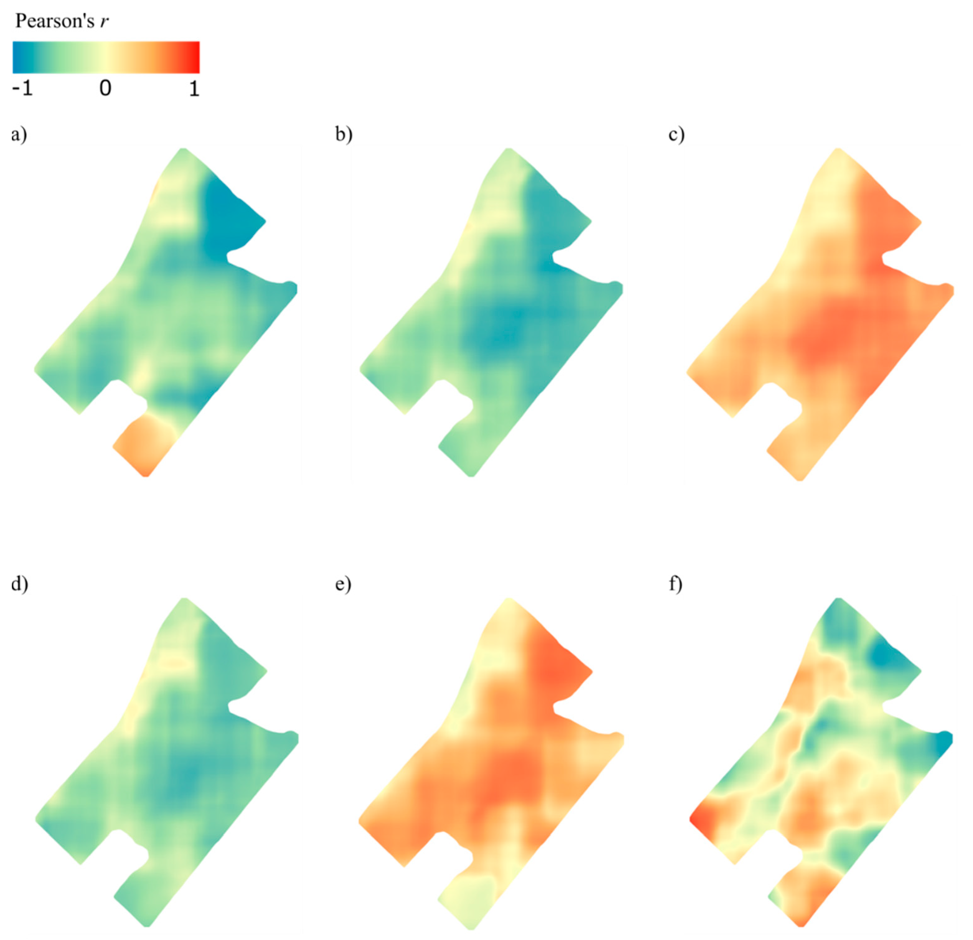
3.2. Localized Correlation Analysis

Localized correlations were calculated to identify feature-specific relationships within the field that may be masked by calculating correlation or regression relationships for the whole field. Mapping these relationships locally provides a spatially distributed maps of the bivariate relationships that may assist in model building. Overall, the localized correlation analysis provided similar general results to the global regression analysis, suggesting that slope, wetness index, relative topographic position and average upslope flow path length have the greatest correlation with crop yield among tested topographic derivatives. The spatial distribution of the Pearson r values was visually inspected to observe the performance of each derivative on features within the field as shown in Figure 3. Although there is significant range in the correlation values across the field, much of the field exhibits similar trends. Areas of the field that are topographically unlike the rest of the field, such as homogenous low-lying areas, appear in contrast to the higher correlations observed in more topographically complex regions of the field. The differences among crop types were insignificant therefore the following descriptions are for the correlations calculated on the raster layer that included the yield anomalies estimated from an average of all crop years.

Slope and TWI (Figure 3b,c, respectively) have similar spatial distributions of correlation values with crop yield, albeit in opposite directions. This similarity should be expected, as wetness index is partially derived from slope. Correlation between crop yield and average upslope flow path length (Figure 3d) also follows similar spatial trends as slope, but experiences slightly reduced correlation values. These three topographic derivatives perform better in regions of greater topographic variation and perform relatively poorly along the flat, low-lying area along the northwest side of the field. This could be due to a threshold relationship between soil moisture and crop yield, where it no longer benefits crop yield to add more moisture after it has become adequately saturated [45,46].

Relative topographic position correlates with yield almost uniformly throughout the field, although to a milder extent than many areas of slope and wetness index. While it does perform best on the largest topographic feature in the field, its performance appears to be the least affected by topographic variation. The difference in its correlation spatial distribution from the other derivatives suggests it may have value in a multi-input GWR without introducing detrimental collinearity. Relative topographic position also appears to be a much better alternative to raw elevation for predicting crop yield, as done in several other studies [3,47]. The in-field region where relative topographic position is the least correlated to yield, the southern corner of the field, is also poorly correlated to other indices. This suggests that poor correlation in this area is due to externally influenced yield anomalies rather than topographically controlled variance. These external factors may be due to the proximity to the roadway, especially compacted soil, or manually modified drainage within that region of the field.

The remaining tested topographic derivatives fail to form any consistent spatial patterns with crop yield, although CVA and the downslope index have small regions where there is noticeable correlation. This limits their potential as independent predictors of crop yield, but these indices may still have utility in multi-input GWR models if they can improve predictions of areas within the field where the more correlated values fail to explain observed variance.

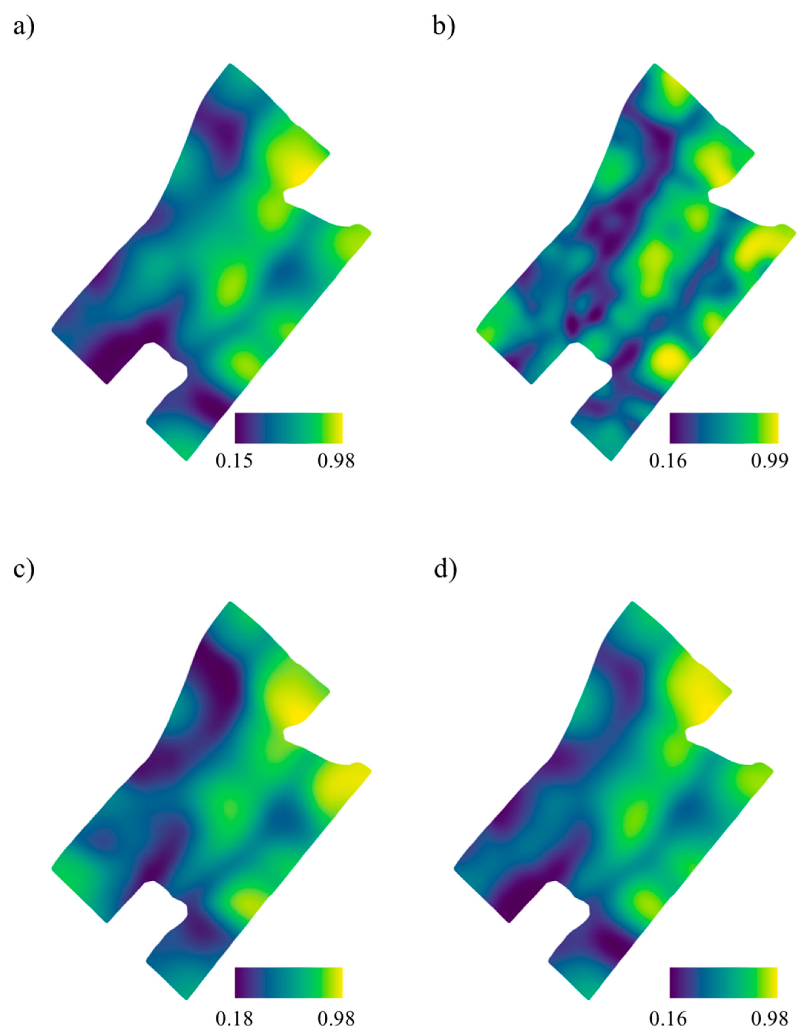
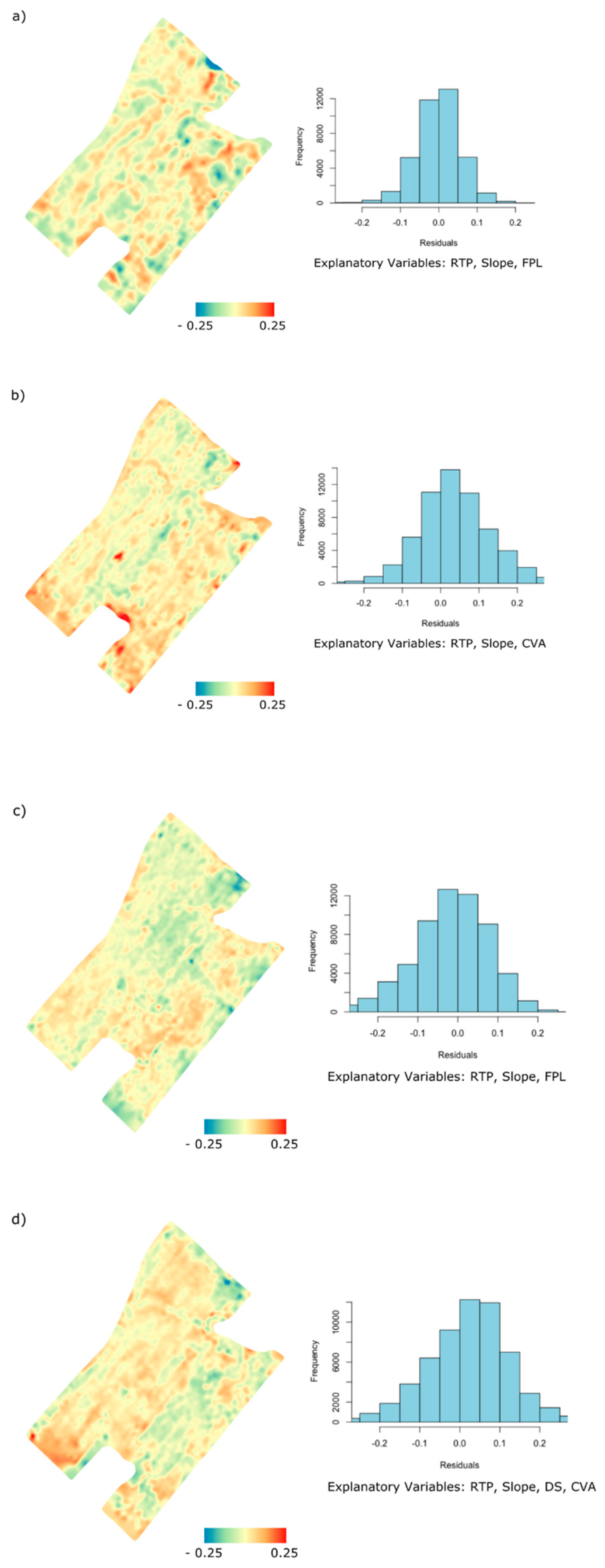
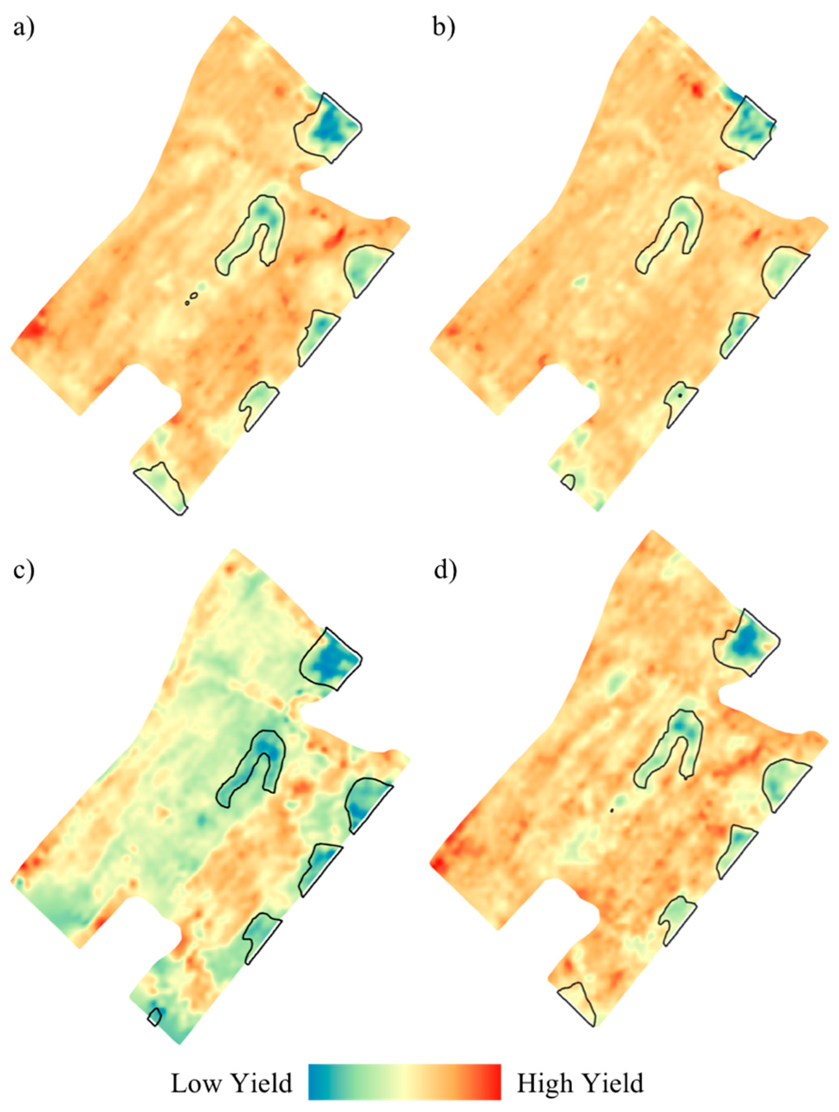
3.3. Crop Yield Predictions

GWR models successfully predicted yield variation within the field, particularly when identifying areas of low yield. The spatial distribution of local coefficient of determination values demonstrates where the models explain the greatest amount of yield variance within the field (Figure 4). It is evident that the local regressions (regressions within the defined moving window) are more effective in topographically variable regions within the field, while the homogenous areas of the field achieved lower R² values. Global coefficient of determination values (determined from an average of all the local relationships) for the corn (R² = 0.80, Root Mean Square Error [RMSE] = 0.088), soy (R² = 0.71, RMSE = 0.073), wheat (R² = 0.73, RMSE = 0.096) and the average of all crops (R² = 0.75) indicate that the models can explain yield variation of all crop types effectively at the whole field scale. This shows that the distribution of the coefficient of determination values and RMSE values do not vary greatly between crop types. The average (standard deviation) of the crop yield for the test years for the specific crops (2018–2016, respectively) in tonnes/ha were 12.5 (1.75) for corn, 3.04 (0.46) for soybeans, and 5.39 (1.41) for wheat. The residuals for all constructed models follow a normal distribution centred around zero, indicating that the models are adequately specified (as shown in Figure 5). In addition to visually inspecting the plotted R² values, residuals for each crop layer were spatially plotted to reveal potential model prediction tendencies related to topographic characteristics (Figure 5).

For predicting crop yield, each GWR model was developed during the model training phase using different combinations of the topographic indices reported in Table 2. The frequency that the selected GWR used a specific topographic index is reported in

Table 4. Frequency of each topographic attribute included in GWR models. There was a total of 4 models one for each crop type and the average of all crop types.

Topographic Attribute	GWR Frequency	Models Used
Relative Topographic Position	4	All Models
Slope	4	All Models
Circular variance of aspect	2	Corn, Soybeans
Upslope Flow Path Length	2	Wheat, Average
Downslope Index	1	Soybeans

. Although the wetness index was determined to be individually correlated with yield variance, it was not included in the any of the constructed models because of its high local and global collinearity with slope and relative topographic position. Relative topographic position and slope were included in each of the created models. The GWR model created to predict corn yield also included circular variance of aspect as an explanatory variable, which boosted prediction accuracy in regions where relative topographic position and slope explained low yield variance. The GWR developed for predicting wheat yields included both circular variance of aspect and downslope index as input variables. Downslope index was only used by the model to predict soybeans yields.

4. Discussion

The results from this study indicate that using specific topographic derivates variables to explain in-field crop yield variation is a valid approach for corn, wheat and soybeans on a topographically variable farm with loamy soils. Ideally, we would have multiple study locations for the identification and evaluation of the important topographic attributes for explaining crop yield variance, however, given the large number of years of yield data and that the data were collected among different crop types, we suggest that the attributes observed are still highly valuable for characterization of yield variance. Further we suggest that the methods employed can be applied more broadly particularly in fields with significant topographic variation. The topographic derivative variables identified as being the most important in explaining crop yield variance were consistent with other findings in the literature [2,4,7]. Relative topographic position, slope, upslope flow path length, circular variance of aspect and the downslope index were the key contributing attributes in predicting crop yield variance. TWI also showed potential as a useful model parameter, but it was not used in this case because of its high collinearity with other variables. Relative topographic position and slope were essential in estimating yield variance for each crop, while circular variance of aspect, average upslope flow path length, and the downslope index were also used to estimate individual crop types. The circular variance of aspect is related to the complexity of surface unlike the remaining variables that are related to topographic position. In our study, the use of secondary derivatives was crucial for the performance of the GWR models. This result emphasizes the importance of their consideration when evaluating surface-related processes and indicates that their continued development may improve future crop yield predictions. Using a GWR approach with these topographic attributes explained nearly 75% of the yield variance over the seven-year study period and successfully identified the bottom-yielding 10% of the study site for each crop type.

The highest-yielding areas of the field were generally well identified by the GWR models (contrast Figure 6 with Figure 4). Perhaps more importantly for improved conservation efforts on farmland [10], the lowest yielding areas of the field (<10%) were correctly classified for all crop types included in the study (Figure 6). The lowest ten percent of each predicted raster layer results in approximately 2 Ha (5 ac) of the field. The regions associated with the lowest yield were typically located on the local high ground of the field (Figure 1). These regions within fields may be unable to produce sufficient yield to offset the cost of growing the crop and therefore may be ideal candidates for alternate land uses [10] or agricultural management approaches. Identifying these regions is important for improving a farm’s overall profitability while conversion of these lands to alternative landcovers such as cover crops or pollination habitat may limit negative environmental impacts. Of the identified low-yielding regions, areas near the perimeter of the farm would be most suitable for alternative land uses as interior regions may be difficult to manage separately from the rest of the field.

In a recent study over the same field, Capmourteres et al. [10] demonstrated that there can be financial and ecological benefits from converting low-yielding regions within a field into alternate land uses (i.e., cover crops, pollination habitat). To be able to identify these areas without having to use crop yield data would be beneficial to farmers, conservationists and governing agencies. It creates an opportunity to evaluate farms owned by smaller operations that may not collect their own crop yield data [48]. Maximizing efficiency is crucial for small farm operations, so being able to provide insight into which areas of the field have topographically limited yield potential may greatly improve their net productivity [49,50]. Severely yield-limited areas within the field may be best suited as an alternate land use, while areas within the field may simply require altered management strategies such as reduced pesticide or nutrient application throughout the growing season.

This concept builds on the rapidly growing idea of heterogeneous farm management, where fields are designated into specific management zones based on their general needs and yield potential [23,51,52,53]. The results of this research show that topography can be used to create easily observable management zones and that their usage may be readily communicated to farmers. This improved communication has the potential to make distinct farm management zones become more widely adopted by farmers. This may be especially true of farmers that are hesitant to invest in precision agriculture technology or do not have the required technological education or experience to operate these systems [54].

Modeling the relative crop yield variability of nearby fields may also improve the assessment of farmland valuation. The market price of farmland can vary greatly through time and location and is often based on the current agricultural economy and recent nearby farm transactions [54]. The largest factor in farmland valuation has traditionally been the available acreage of workable ground. The heterogeneity of yield potential within a field is often overlooked as each hectare within the field is essentially considered equal. The ability to quickly and remotely assess the spatial variance of crop yield potential through the use of topographic variables may improve the accuracy of its valuation.

Considerations must be made for how these results may translate to other farms and landscapes. The farm in this study is managed by farmers that have access to modern agricultural equipment and accurate agronomic information. When common yield limiting factors such as poor soil quality and human error are reduced, it places greater importance on surface water and nutrient availability. Therefore, well-managed farms may see a stronger relationship between topography and crop yield. The relationship would also likely be weaker on farms with less topographic variation. The most utilized derivatives in this research were relative topographic position and slope. With fewer sloping terrains and more flat regions, there would naturally be less topographic control of surface water movement. This would likely decrease the explanatory power of these variables. Accounting for systematic drainage and using different topographic derivatives may be useful in trying to predict crop yield with topographic variables in these types of fields [55]. Another approach to address this potential issue in less topographically variable fields may be to identify and utilize multiscale derivatives that consider the topography at several different scales [38].

This research shows mild differences in predictive ability between crop types, but these differences may be greater in regions where entirely different crops are grown. Corn, soybeans and winter wheat can generally be grown in the same region because of their similar soil and temperature requirements. In areas where the topography and soil type does not permit the successful growth of these crops, and other crop types are grown instead, there may be large differences in the ability of topographic derivatives to predict yield variation within a field. This highlights the need to individually test potential input variables for a multi-input models such as the GWR. Further research may explore other spatial prediction models, for example, several researchers suggest that GWR approaches are more useful for the identification of stationarity in spatial distributed data [56,57], rather than for spatial prediction, therefore, other approaches such as those which combine GWR with more complex spatial models such as GWR combined with kriging [58] may provide more reliable spatial models.

5. Conclusions

The results of this work suggest that topographic attributes should be considered to identify relationships among crop yield and within-field topographic variations. This study, which included multiple years of yield data for several cereal crops demonstrated that topographic derivatives such as relative topographic position proved to be more predictive than elevation, which has been included in past studies investigating relationships between topography and crop yield. Additionally, this study shows that localized relationships between topographic derivatives and yield, such as those determined using GWR results in much better predictions than those which would be derived from generalized relationships determined from the full field. Therefore, crop yield predictions should consider local topography especially as fine-resolution topographic data become more accessible through new aerial-based sensor technologies, such as LiDAR. Testing these methods in different environments with other crops and soil types is advised to reveal more information about topography–crop yield relationships and ensure that these results are transferable to other regions.

References

1. Ferris, J.L. Data privacy and protection in the agriculture industry: Is federal regulation necessary. Minn. JL Sci. Tech. 2017, 18, 309. [Google Scholar]
2. Green, T.R.; Salas, J.D.; Martinez, A.; Erskine, R.H. Relating crop yield to topographic attributes using Spatial Analysis Neural Networks and regression. Geoderma 2007, 139, 23–37. [Google Scholar] [CrossRef]
3. Jiang, P.; Thelen, K.D. Effect of Soil and Topographic Properties on Crop Yield in a North-Central Corn-Soybean Cropping System. Agronomy J. 2004, 96, 252–258. [Google Scholar] [CrossRef]
4. Kumhálová, J.; Kumhála, F.; Kroulík, M.; Matějková, Š. The impact of topography on soil properties and yield and the effects of weather conditions. Precis. Agric. 2011, 12, 813–830. [Google Scholar] [CrossRef]
5. Heil, K.; Heinemann, P.; Schmidhalter, U. Modeling the Effects of Soil Variability, Topography, and Management on the Yield of Barley. Front. Environ. Sci. 2018, 6, 146. [Google Scholar] [CrossRef]
6. Si, B.C.; Farrell, R.E. Scale-Dependent Relationship between Wheat Yield and Topographic Indices: A Wavelet Approach. Soil Sci. Soc. Am. J. 2004, 68, 577–587. [Google Scholar] [CrossRef]
7. Kaspar, T.C.; Colvin, T.S.; Jaynes, D.B.; Karlen, D.L.; James, D.E.; Meek, D.W.; Pulido, D.; Butler, H. Relationship between six years of corn yields and terrain attributes. Precis. Agric. 2003, 1, 87–101. [Google Scholar] [CrossRef]
8. Wei, T.; Cherry, T.L.; Glomrød, S.; Zhang, T. Climate change impacts on crop yield: Evidence from China. Sci. Total Environ. 2014, 499, 133–140. [Google Scholar] [CrossRef] [Green Version]
9. Whitcomb, J.; Clewley, D.; Colliander, A.; Cosh, M.H.; Powers, J.; Friesen, M.; McNairn, H.; Berg, A.A.; Bosch, D.D.; Coffin, A.; et al. Evaluation of SMAP Core Validation Site Representativeness Errors using Dense Networks of in situ Sensors and Random Forests. IEEE J. Select. Top. Appl. Earth Observ. Remote Sens. 2020, 13, 6457–6472. [Google Scholar] [CrossRef]
10. Capmourteres, V.; Adams, J.; Berg, A.; Fraser, E.; Swanton, C.; Anand, M. Precision conservation meets precision agriculture: A case study from southern Ontario. Agric. Syst. 2018, 167, 176–185. [Google Scholar] [CrossRef]
11. Lanni, C.; McDonnell, J.J.; Rigon, R. On the relative role of upslope and downslope topography for describing water flow path and storage dynamics: A theoretical analysis. Hydrol Proc. 2011, 25, 3909–3923. [Google Scholar] [CrossRef]
12. Moeslund, J.E.; Arge, L.; Bøcher, P.K.; Dalgaard, T.; Ejrnæs, R.; Odgaard, M.V.; Svenning, J.-C. Topographically controlled soil moisture drives plant diversity patterns within grasslands. Biodivers. Conserv. 2013, 22, 2151–2166. [Google Scholar] [CrossRef]
13. Wolock, D.M.; Hornberger, G.M.; Musgrove, T.J. Topographic effects on flow path and surface water chemistry of the Llyn Brianne catchments in Wales. J. Hydrol. 1990, 115, 243–259. [Google Scholar] [CrossRef]
14. Ghandehari, M.; Buttenfield, B.P.; Farmer, C.J.Q. Comparing the accuracy of estimated terrain elevations across spatial resolution. Int. J. Remote Sens. 2019, 40, 5025–5049. [Google Scholar] [CrossRef]
15. McKinion, J.M.; Willers, J.L.; Jenkins, J.N. Spatial analyses to evaluate multi-crop yield stability for a field. Comput. Electron. Agric. 2010, 70, 187–198. [Google Scholar] [CrossRef]
16. Statistics Canada. 2016 Census of Agriculture. Available online: https://www150.statcan.gc.ca/n1/daily-quotidien/170510/dq170510a-eng.htm (accessed on 4 May 2020).
17. Laamrani, A.; Voroney, P.R.; Berg, A.A.; Gillespie, A.W.; March, M.; Deen, B.; Martin, R.C. Temporal Change of Soil Carbon on a Long-Term Experimental Site with Variable Crop Rotations and Tillage Systems. Agronomy 2020, 10, 840. [Google Scholar] [CrossRef]
18. Hoffman, D.W.; Matthews, B.C.; Wicklund, R.E. Soil Associations of Southern Ontario; Report No. 30 of the Ontario Soil Survey; Canada Department of Agriculture: Ottawa, ON, Canada, 1964. [Google Scholar]
19. Laamrani, A.; Berg, A.A.; Voroney, P.; Feilhauer, H.; Blackburn, L.; March, M.; Dao, P.D.; He, Y.; Martin, R.C. Ensemble Identification of Spectral Bands Related to Soil Organic Carbon Levels over an Agricultural Field in Southern Ontario, Canada. Remote Sens. 2019, 11, 1298. [Google Scholar] [CrossRef] [Green Version]
20. Kharel, T.P.; Maresma, A.; Czymmek, K.J.; Oware, E.K.; Ketterings, Q.M. Combining spatial and temporal corn silage yield variability for management zone development. Agron. J. 2019, 111, 2703–2711. [Google Scholar] [CrossRef]
21. Meng, Q.; Liu, Z.; Borders, B.E. Assessment of regression kriging for spatial interpolation-comparisons of seven GIS interpolation methods. Cartogr. Geogr. Inf. Sci. 2013, 40, 28–39. [Google Scholar] [CrossRef]
22. Hutchinson, M.F.; Gessler, P.E. Splines-more than just a smooth interpolator. Geoderma 1994, 62, 45–67. [Google Scholar] [CrossRef]
23. Lauzon, J.D.; Fallow, D.J.; O’Halloran, I.P.; Gregory, S.D.L.; von Bertoldi, A.P. Assessing the temporal stability of spatial patterns in crop yields using combine yield monitor data. Can. J. Soil Sci. 2005, 85, 439–451. [Google Scholar] [CrossRef]
24. Varvel, G.E. Crop rotation and nitrogen effects on normalized grain yields in a long-term study. Agron. J. 2000, 92, 938–941. [Google Scholar] [CrossRef] [Green Version]
25. Al-Gaadi, K.A.; Hassaballa, A.A.; Tola, E.; Kayad, A.G.; Madugundu, R.; Assiri, F.; Alblewi, B. Characterization of the spatial variability of surface topography and moisture content and its influence on potato crop yield. Int. J. Remote Sens. 2018, 39, 8572–8590. [Google Scholar] [CrossRef]
26. Kravchenko, A.N.; Bullock, D.G. Correlation of Corn and Soybean Grain Yield with Topography and Soil Properties. Agron. J. 2000, 92, 75–83. [Google Scholar] [CrossRef]
27. Maestrini, B.; Basso, B. Predicting spatial patterns of within-field crop yield variability. Field Crop. Res. 2018, 219, 106–112. [Google Scholar] [CrossRef]
28. Wilson, J.P.; Gallant, J.C. (Eds.) Terrain Analysis: Principles and Applications; John Wiley & Sons: Hoboken, NJ, USA, 2000. [Google Scholar]
29. Schmidt, J.P.; Hong, N.; Dellinger, A.; Beegle, D.B.; Lin, H.S. Hillslope variability in corn response to nitrogen linked to in-season soil moisture redistribution. Agron. J. 2007, 99, 229–237. [Google Scholar] [CrossRef] [Green Version]
30. Moore, I.D.; Grayson, R.B.; Ladson, A.R. Digital terrain modelling: A review of hydrological, geomorphological, and biological applications. Hydrol. Process. 1991, 5, 3–30. [Google Scholar] [CrossRef]
31. Lindsay, J.B. Whitebox GAT: A case study in geomorphometric analysis. Comput. Geosci. 2016, 95, 75–84. [Google Scholar] [CrossRef]
32. Grohmann, C.H.; Smith, M.J.; Riccomini, C. Multiscale analysis of topographic surface roughness in the Midland Valley, Scotland. IEEE Trans. Geosci. Remote Sens. 2010, 49, 1200–1213. [Google Scholar] [CrossRef] [Green Version]
33. Oleg, A.; Hatic, D.; Pernar, R. DEM-based depth in sink as an environmental estimator. Ecol. Model. 2001, 138, 247–254. [Google Scholar]
34. Hjerdt, K.N.; McDonnell, J.J.; Seibert, J.; Rodhe, A. A new topographic index to quantify downslope controls on local drainage. Water Resour. Res. 2004, 40. [Google Scholar] [CrossRef] [Green Version]
35. Freeman, T.G. Calculating catchment area with divergent flow based on a regular grid. Comput. Geosci. 1991, 17, 413–422. [Google Scholar] [CrossRef]
36. Gudim, S. Impoundment Size Index (ISI): The use of potential impoundment size for the characterization of topographic incision in DEMs. MSc Thesis, Presented to the University of Guelph, Guelph, ON, Canada, 2019. [Google Scholar]
37. Gallant, J.C. Primary topographic attributes. In Terrain Analysis-Principles and Application; Wilson, J.P., Gallant, J.C., Eds.; John Wiley & Sons: Hoboken, NJ, USA, 2000; pp. 51–86. [Google Scholar]
38. Newman, D.R.; Lindsay, J.B.; Cockburn, J.M.H. Evaluating metrics of local topographic position for multiscale geomorphometric analysis. Geomorphology 2018, 312, 40–50. [Google Scholar] [CrossRef]
39. Beven, K.J.; Kirkby, M.J. A physically based, variable contributing area model of basin hydrology. Hydrol. Sci. Bull. 1979, 24, 43–69. [Google Scholar] [CrossRef] [Green Version]
40. Team, R. Core. R: A Language and Environment for Statistical Computing; R foundation for Statistical Computing: Vienna, Austria, 2013. [Google Scholar]
41. Robertson, C.; Long, J.A.; Nathoo, F.S.; Nelson, T.A.; Plouffe, C.C.F. Assessing Quality of Spatial Models Using the Structural Similarity Index and Posterior Predictive Checks: Assessing Quality of Spatial Models. Geogr. Anal. 2014, 46, 53–74. [Google Scholar] [CrossRef] [Green Version]
42. Tsutsumida, N.; Rodríguez-Veiga, P.; Harris, P.; Balzter, H.; Comber, A. Investigating spatial error structures in continuous raster data. Int. J. Appl. Earth Obs. Geoinf. 2019, 74, 259–268. [Google Scholar] [CrossRef]
43. Matthews, S.A.; Yang, T.-C. Mapping the results of local statistics: Using geographically weighted regression. Demogr. Res. 2012, 26, 151–166. [Google Scholar] [CrossRef] [Green Version]
44. Tu, J.; Xia, Z. Examining spatially varying relationships between land use and water quality using geographically weighted regression I: Model design and evaluation. Sci. Total Environ. 2008, 407, 358–378. [Google Scholar] [CrossRef]
45. Foody, G.M. Geographical weighting as a further refinement to regression modelling: An example focused on the NDVI–rainfall relationship. Remote Sens. Environ. 2003, 88, 283–293. [Google Scholar] [CrossRef]
46. Musick, J.T.; Jones, O.R.; Stewart, B.A.; Dusek, D.A. Water-Yield Relationships for Irrigated and Dryland Wheat in the U.S. Southern Plains. Agron. J. 1994, 86, 980–986. [Google Scholar] [CrossRef]
47. Thompson, R.B.; Gallardo, M.; Valdez, L.C.; Fernández, M.D. Using plant water status to define threshold values for irrigation management of vegetable crops using soil moisture sensors. Agric. Water Manag. 2007, 88, 147–158. [Google Scholar] [CrossRef]
48. Paustian, M.; Theuvsen, L. Adoption of precision agriculture technologies by German crop farmers. Precis. Agric. 2017, 18, 701–716. [Google Scholar] [CrossRef]
49. Schilling, B.J.; Attavanich, W.; Sullivan, K.P.; Marxen, L.J. Measuring the effect of farmland preservation on farm profitability. Land Use Policy 2014, 41, 84–96. [Google Scholar] [CrossRef]
50. Mottaleb, K.A.; Mohanty, S. Farm size and profitability of rice farming under rising input costs. J. Land Use Sci. 2015, 10, 243–255. [Google Scholar] [CrossRef]
51. Bullock, D.S.; Boerngen, M.; Tao, H.; Maxwell, B.; Luck, J.D.; Shiratsuchi, L.; Puntel, L.; Martin, N.F. The Data-Intensive Farm Management Project: Changing Agronomic Research Through On-Farm Precision Experimentation. Agron. J. 2019, 111, 2736–2746. [Google Scholar] [CrossRef] [Green Version]
52. Buttafuoco, G.; Castrignanò, A.; Cucci, G.; Lacolla, G.; Lucà, F. Geostatistical modelling of within-field soil and yield variability for management zones delineation: A case study in a durum wheat field. Precis. Agric. 2017, 18, 37–58. [Google Scholar] [CrossRef]
53. Mzuku, M.; Khosla, R.; Reich, R.; Inman, D.; Smith, F.; MacDonald, L. Spatial Variability of Measured Soil Properties across Site-Specific Management Zones. Soil Sci. Soc. Am. J. 2005, 69, 1572–1579. [Google Scholar] [CrossRef] [Green Version]
54. Mittal, S.; Mehar, M. Socio-economic Factors Affecting Adoption of Modern Information and Communication Technology by Farmers in India: Analysis Using Multivariate Probit Model. J. Agric. Educ. Ext. 2016, 22, 199–212. [Google Scholar] [CrossRef]
55. Wang, H. The Spatial Structure of Farmland Values: A Semiparametric Approach. Agric. Resour. Econ. Rev. 2018, 47, 568–591. [Google Scholar] [CrossRef] [Green Version]
56. Gollini, I.; Lu, B.; Charlton, M.; Brunsdon, C.; Harris, P. GWmodel: An R package for exploring spatial heterogeneity using geographically weighted models. arXiv 2013, arXiv:1306.0413. [Google Scholar] [CrossRef] [Green Version]
57. Lu, B.; Charlton, M.; Harris, P.; Fotheringham, A.S. Geographically weighted regression with a non-Euclidean distance metric: A case study using hedonic house price data. Int. J. Geogr. Inf. Sci. 2014, 28, 660–681. [Google Scholar] [CrossRef]
58. Harris, P.; Fotheringham, A.S.; Crespo, R.; Charlton, M. The use of geographically weighted regression for spatial prediction: An evaluation of models using simulated data sets. Math. Geosci. 2010, 42, 657–680. [Google Scholar] [CrossRef]
Figure 1. Maps showing the location of the study site in (A) southwestern Ontario within (B) the Lake Erie basin. (C) The study site with a topographic overview, adapted from [19].
Remotesensing 13 04152 g001
Figure 2. Map illustrating high and low yielding regions for 2017 crop year (a). The yields are expressed from a standardized anomaly (Equation (1)) from a mean of 3.04 and standard deviation of 0.46 tonnes/ha. In (b) the yield data removed (based on the criteria described in Section 2.2) are shown in gray.
Remotesensing 13 04152 g002
Figure 3. Correlation coefficients between study period average crop yield and (a) relative topographic position; (b) slope; (c) Wetness Index; (d) upslope flow path length; (e) Downslope Index; (f) CVA.
Remotesensing 13 04152 g003
Figure 4. Spatial patterns of R2 for (a) all crops; (b) corn; (c) winter wheat; (d) soybeans.
Remotesensing 13 04152 g004
Figure 5. Spatially plotted predicted crop yield residuals and included explanatory variables for (a) average of all crops; (b) corn; (c) winter wheat; (d) soybeans.
Remotesensing 13 04152 g005
Figure 6. Normalized observed crop yield data for (a) study period average; (b) corn; (c) winter wheat; (d) soybeans. Black outline polygons indicate GWR predicted lowest 10 percent of crop yield.
Remotesensing 13 04152 g006