Article

TRS: Transformers for Remote Sensing Scene Classification

1
College of Computer Science and Technology, Jilin University, Changchun 130012, China
2
Key Laboratory of Symbolic Computation and Knowledge Engineering of Ministry of Education, Jilin University, Changchun 130012, China
3
Department of Jilin University Library, Jilin University, Changchun 130012, China
*
Author to whom correspondence should be addressed.
Remote Sens. 2021, 13(20), 4143; https://doi.org/10.3390/rs13204143
Submission received: 11 September 2021 / Revised: 11 October 2021 / Accepted: 13 October 2021 / Published: 16 October 2021
(This article belongs to the Special Issue Deep Learning for Remote Sensing Image Classification)

Abstract

:
Remote sensing scene classification remains challenging due to the complexity and variety of scenes. With the development of attention-based methods, Convolutional Neural Networks (CNNs) have achieved competitive performance in remote sensing scene classification tasks. As an important method of the attention-based model, the Transformer has achieved great success in the field of natural language processing. Recently, the Transformer has been used for computer vision tasks. However, most existing methods divide the original image into multiple patches and encode the patches as the input of the Transformer, which limits the model’s ability to learn the overall features of the image. In this paper, we propose a new remote sensing scene classification method, Remote Sensing Transformer (TRS), a powerful “pure CNNs → Convolution + Transformer → pure Transformers” structure. First, we integrate self-attention into ResNet in a novel way, using our proposed Multi-Head Self-Attention layer instead of 3 × 3 spatial revolutions in the bottleneck. Then we connect multiple pure Transformer encoders to further improve the representation learning performance completely depending on attention. Finally, we use a linear classifier for classification. We train our model on four public remote sensing scene datasets: UC-Merced, AID, NWPU-RESISC45, and OPTIMAL-31. The experimental results show that TRS exceeds the state-of-the-art methods and achieves higher accuracy.

1. Introduction

With the rapid development of remote sensing technology and the emergence of more sophisticated remote sensing sensors, remote sensing technologies have been widely used in various fields [1,2,3,4]. As one of the core tasks of remote sensing, remote sensing scene classification is often used as a benchmark to measure the understanding of remote sensing scene images. The progress of remote sensing scene classification often promotes the improvement of other related tasks, such as remote sensing image retrieval and target detection [1,2].
The traditional remote sensing scene classification method mainly relies on the spatial features of images [5,6]. However, the error rate is high in the complex remote sensing scene. In recent years, many deep convolutional neural network models have made significant progress in remote sensing scene classification with the development of deep learning. The convolution operation can effectively obtain the local information of the image. The authors of [7,8] proved that different features can be extracted by convolutional layers of different depths. To aggregate global features, neural networks based on convolution operations need to stack multiple layers [9]. He et al. [10] proposed ResNet to make Convolutional Neural Networks(CNNs) deeper and easier to train. However, Liang et al. [11] suggested that only relying on a fully connected layer to complete the classification ignores the features of different convolutional layers in CNNs. Compared with stacking more layers to improve the accuracy of remote sensing scene classification, it is a more effective way to establish the relationship between local information through the attention mechanism.
The self-attention-based structure proposed in Transformer [12] is dominant in natural language processing (NLP) tasks. Self-attention can learn abundant features from long-sequence data and establish the dependency relationship between different features. Bert and GPT [13,14,15,16] were proposed based on Transformer architecture. Inspired by the success of NLP, many researchers applied self-attention to computer vision tasks. Wang et al. [17] and Ramachandran et al. [18] proposed a special attention mode to completely replace convolution operation, but it has not been extended to modern hardware accelerators. SENet [19], CBAM [20], SKNet [21], and Non-Local Net [22] combine self-attention with CNNs (such as ResNet). However, convolution operations are still the core of these methods, and self-attention is added to the bottleneck structure in the form of additional modules. Recently, Transformer architecture applications to computer vision tasks have shown great prospects. Dosovitskiy et al. [23] proposed the Vision Transformer (ViT). The ViT directly inputs the image into the standard Transformer encoder, which can learn the dependencies of different positions of the image well, but ignores the overall semantic features of the image, and the accuracy of ViT is only close to that of CNNs. Several works have also used the “Convolution + Transformer” structure. Touvron et al. [24] used knowledge distillation technology to allow CNN to assist in training the ViT, but this made training difficult. Carion et al. [25] proposed end-to-end DETR. DETR uses CNNs as the backbone to extract features and connects with Transformers to complete object detection. However, DETR has not been proven to be good for image classification.
Due to the lack of inductive bias [25,26], the number of images in the remote sensing scene dataset is not enough for the Transformer to achieve good results without the ImageNet1K pre-trained model. Therefore, we need to combine CNNs with Transformers. The existing “Convolution + Transformer” models reshape the outputs of the CNN backbone and connect them with Transformers. We believe that the existing models ignore the information contained in the three-dimensional representations of images. Therefore, we aim to design a Transformer capable of processing the three-dimensional matrix as a transition module between CNNs and standard Transformers. We are surprised to find the unique relationship between the standard bottleneck structure and the Transformer architecture (for details, see Section 3.4). Therefore, we propose the MHSA-Bottleneck.
In this paper, we develop a remote sensing Transformer (TRS) based on ResNet50 and Transformer architecture, which significantly boosts the remote sensing scene classification performance and reduces the dependence of the model on convolution operation. We propose a novel “pure CNNs → Convolution + Transformer → pure Transformers” structure. Different from the conventional “Convolution + Transformer” method, we do not simply connect the CNNs and Transformers, but integrate the Transformers into CNNs. We replace the last three bottlenecks of ResNet50 with multiple Transformer encoders and design the MHSA-Bottleneck. We replace the 3 × 3 spatial convolutions in the bottleneck with position-encoded Multi-Head Self-Attention rather than using the attention mechanism as an auxiliary module to the convolution module. Our contribution is not only the successful application of Transformers to remote sensing classification tasks, but also the provision of a special way to understand bottleneck structure.
We summarize our contributions as follows:
(1)
We apply the Transformer to remote sensing scene classification, and propose a novel “pure CNNs → CNN + Transformer → pure Transformers” structure called TRS. The TRS can well combine Transformers with CNNs to achieve better classification accuracy.
(2)
We propose the MHSA-Bottleneck. The MHSA-Bottleneck uses Multi-Head Self-Attention instead of the 3 × 3 spatial convolutions. The MHSA-Bottleneck has fewer parameters and better effects than the standard bottleneck and other bottlenecks improved by the attention mechanism.
(3)
We also provide a novel way to understand the structure of the bottleneck. We demonstrate the connection between the MHSA-Bottleneck and Transformer, and regard MHSA- Bottleneck as a 3D Transformer.
(4)
We complete training on four public datasets NWPU-RESISC45, UC-Merced, AID, and OPTIMAL-31. The experimental results prove that TRS surpasses the existing state-of-the-art CNNs methods.
The rest of this paper is organized as follows. Section 2 introduces our related work, and Section 3 introduces the structure and algorithm of the TRS in detail. The ablation study and state-of-the-art comparison are shown in Section 4. Section 5 presents the conclusion of our article.

2. Related Works

2.1. CNNs in Remote Sensing Scene Classification

CNNs have been the dominant method of image classification, since AlexNet [27] won the ImageNet competition in 2012. The emergence of various CNNs has made a great contribution to the improvement of image classification accuracy. These deep models also demonstrate good performance on remote sensing datasets. Cheng et al. [28] fine-tuned AlexNet [27], GoogleNet [29], VGGNet [9], etc., and proposed a benchmark for remote sensing scene classification. Due to the excellent performance of the optimized VGG-16 [30], it is often used as the backbone for feature extraction. The ResNet [10] increases the depth of the network, reduces the model parameters, and improves the training speed by using residual modules. EfficientNet [31] balanced the depth and width of the network to obtain a better result. Bi et al. [32] proposed an Attention Pooling-based Dense Connected Convolutional Neural Network (APDC-Net) as the backbone and adopted a multi-level supervision strategy. Hu et al. [33] believed that the abundance of prior information was an important factor that affected the accuracy of remote sensing scene classification, and proposed to pre-train the model on ImageNet. Li et al. [34] used different convolutional layers of a pre-trained CNN to extract information. Zhang et al. [35] proposed the Gradient Boosting Random Convolutional Network (GBRCN), which selected different deep convolutional neural network models for different remote sensing scenes. The problem with the CNNs is that they can only focus on the local information of the size of each convolution kernel. In order to solve this problem, GBNet [36] integrated layered feature aggregation into an end-to-end network. Xu et al. [37] proposed the Lie Group Regional Influence Network (LGRIN) which combined the lie group machine learning with CNNs and achieved state-of-the-art.

2.2. Attention in CNNs

Although integrating multi-layer features and increasing the depth of the network can improve the classification accuracy, it is clearly a better choice to use local information to establish dependencies. The attention mechanism is widely used to obtain global information of CNNs. For example, Wang et al. [38] proposed a “CNN + LSTM” model in ARCNet, which used LSTM to replace feature fusion to establish connections between multiple layers. Yu et al. [39] present Attention GANs. Attention GANs are optimized with attention and input the learned features into SVM [40,41,42] or KNN [43,44,45,46,47,48,49,50] for classification. There are also methods to optimize the bottleneck of ResNet with unique self-attention. SENet [19] proposes the Squeeze-and-Excitation (SE) module to learn the relationship between channels. The Squeeze operation in the SE module is used to obtain the channel-level global features from the feature map. Then, the SE module performs an Excitation operation on the global features. CBAM [20] adds spatial attention based on SENet. Non-Local Net [22] combines the Transformer and Non-Local algorithms to capture remote dependencies through global attention. ResNeSt [51] introduces the Split-Attention block to realize multi-layer feature-map attention. There are three differences between the MHSA-Bottleneck and bottleneck optimized by the above methods: (1) Compared with Non-Local Net, the MHSA-Bottleneck uses multiple head vectors and adds position embedding. (2) The MHSA-Bottleneck uses Multi-Head Self-Attention instead of the 3 × 3 spatial convolutions. SENet, CBAM, and Non-local Net are usually added to the bottleneck structure in the form of additional modules, which increase the model parameters and calculation cost. (3) The convolution mechanism is still the core of SENet, CBAM, Non-local Net, and ResNeSt. The MHSA-Bottleneck deletes the 3×3 space convolutions and relies on Multi-Head Self-Attention for learning.

2.3. Transformer in Vision

The Transformer was originally proposed by [12] for natural language processing tasks. Self-attention was introduced in the Transformer, which has the advantage of performing global calculations on input sequences and summarizing the information for an update. In the fields of NLP and speech recognition, Transformers are replacing Recurrent Neural Networks [52,53,54,55]. Recently, several works have applied the Transformer to computer vision. Parmar et al. [56] initially used each pixel of the image as the input of the Transformer, which greatly increased computational cost. Child et al. [57] proposed Sparse Transformers which are scalable modules suitable for image processing tasks. Vision Transformer [23] divided a picture into multiple patches as input of the model, and the size of each patch was 16 × 16 or 14 × 14. However, the ViT ignores the overall semantic features of the image and requires additional datasets to assist training [58]. Bello et al. [59] proposed a combination of CNNs and Transformers. DETR [25] used Transformers to further process the 2D image representation output by CNNs. Tokens-to-Token (T2T) ViT [60] designed a deep and narrow structure for the backbone, and proposed a “Tokens-to-Token module” to model local information. DieT [24] used the T2T for reference and uses knowledge distillation [61,62] to improve the original ViT. The PVT [25] combines convolution and the ViT to make it more suitable for downstream tasks. The Swin Transformer [63] uses window attention to combine global and local information, and it is one of the best models. However, the Swin Transformer and PVT still lack inductive bias and need a large number of datasets to complete training. Recently, many researchers have applied Transformer to remote sensing tasks. MSNet [64] proposes a network fusion method for Remote Sensing Spatiotemporal Fusion. Bazi et al. [65] use the structure of the ViT to remote sensing scene classification. Xu et al. [66] combine the Swin Transformer and UperNet for remote sensing image segmentation. These methods all migrate the existing Transformer structure to remote sensing tasks, and the lack of inductive bias is not resolved.

3. Methodology

3.1. Overview of TRS

The design of the TRS is based on ResNet50 architecture, which consists of four parts: the stem unit, standard bottleneck, MHSA-Bottleneck, and Transformer encoder. Figure 1 demonstrates the overall architecture of the TRS. First, we used CNNs (stem unit + bottleneck) and the MHSA-Bottleneck to learn the 3D representation of input images. Then, we added position embedding and class token to the representation and passed it to the Transformer encoders. Finally, a linear classifier is used to complete the classification. The details of the model are described in Table 1.

3.2. Stem Unit

CNNs usually start from a stem unit that can quickly reduce image resolution. Similar to ResNet50, TRS starts with a 7 × 7 convolution kernel, stride-2, and three zero-padding layers. As the Transformer has strict restrictions on the input data, different convolution operations were selected for images in different sizes. For example, when the resolution of the remote sensing image was 600 × 600, we used two 7 × 7 convolution kernels with the stride of 5 and 1, respectively, as the stem unit.

3.3. Transformer Architecture

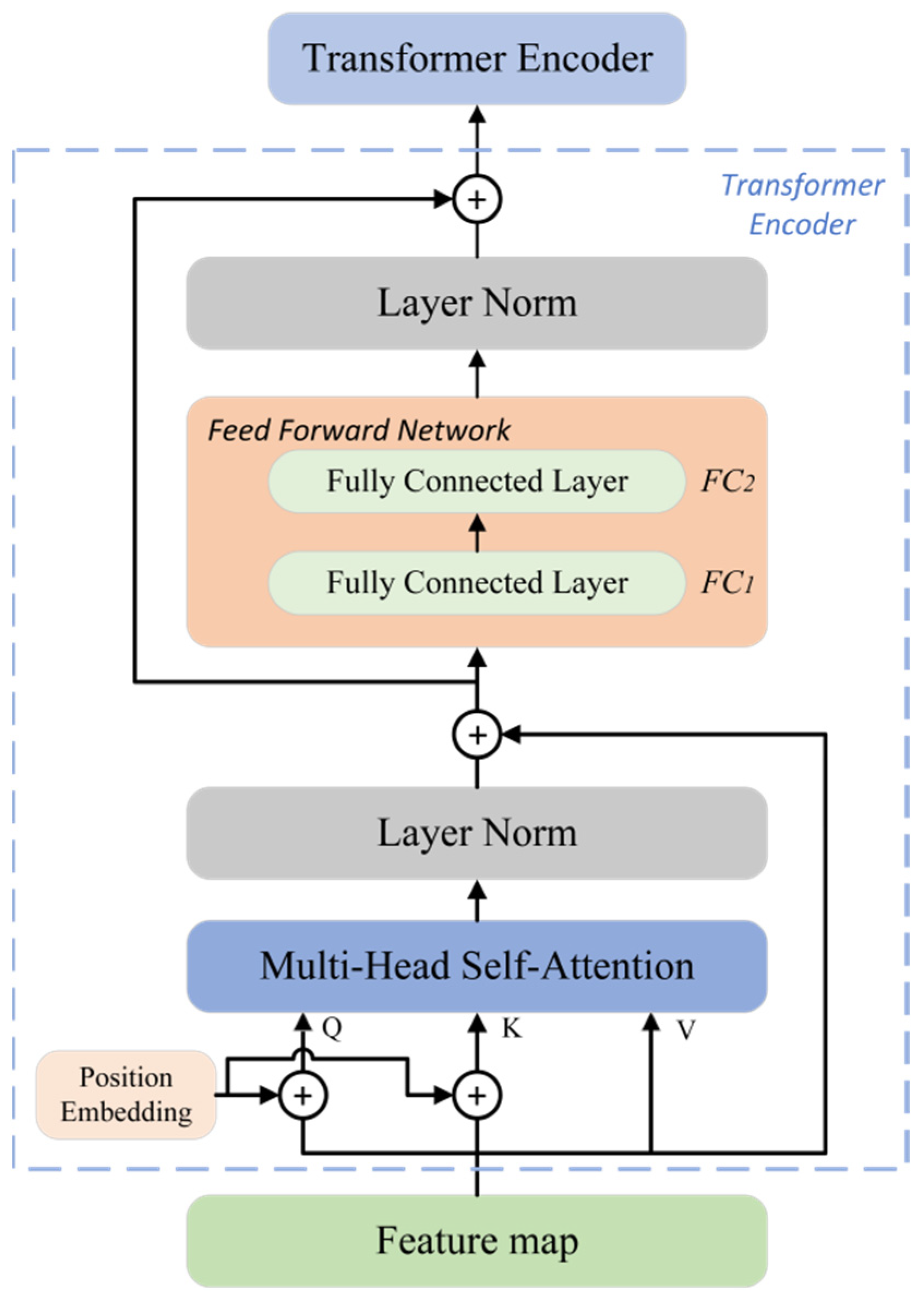
We only chose the Transformer encoder as a component of the TRS. As shown in Figure 2, the overall Transformer encoder architecture consists of three parts: Multi-Head Self-Attention, position embedding, and the feed-forward network.
Multi-Head Self-Attention: Multi-Head Self-Attention is an important component for modeling the relationship between feature representations in the Transformer. As shown in Table 1, the output of Stage4 (S4) was I = (14, 14, 1024). We put I into a convolution kernel with a kernel size of 1 × 1 to get I’= (14, 14, d). We added the class token to I’ and flattened the first two dimensions. Then, we obtained N d-dimensional vectors as the input of the Transformer encoder (N = 14 × 14 + 1). M = (N, d) denotes the input of the Transformer. The self-attention layer, as proposed in [14] which uses the query, key and value matrix (QKV) to train the associative memory. The calculation method of the QKV matrix is shown as follows:
Q = M × W Q Τ K = M × W K Τ V = M × W V Τ ,
where WQ, WK, and WV are trainable matrices. We use the inner product to match the Q matrix and the K matrix, and used d1/2 to complete the normalization. Then, we used the Softmax function to process the normalized inner product result. The output of self-attention is expressed as:
A t t e n t i o n ( Q , K , V ) = S o f t m a x ( Q K Τ d ) V ,
The authors of [14] proved that multiple attention heads can learn detailed information and improve classification performance. Multi-Head Self-Attention involves dividing Q, K, and V into several attention heads. We set the number of attention heads as h, d’ = d/h. We used h heads of size (N, d’) for calculation according to (2). Finally, we remapped the output matrix to (N, d).
Position Embedding: The self-attention structure in the Transformer cannot capture the order of the input sequence. Thus, we used position embedding to supplement the position information of the remote sensing image [14]. Since different functions should be used to complete position encoding in different dimensions, we used the Cosine function and the Sine function to calculate the absolute position according to the odd and even dimensions of the vector, respectively. The specific calculation method of position embedding is as follows:
P E ( p o s , 2 i ) = s i n ( p o s λ 2 i / d ) P E ( p o s , 2 i + 1 ) = c o s ( p o s λ 2 i / d ) ,
which meets posN, id. λ is a hyperparameter that controls the wavelength of the periodic function. Position embedding was added to the Q and K matrices.
Feedforward networks (FNN): FNN is composed of two fully connected layers: FC1 and FC2. FC1 changes the input dimension from (N, d) to (N, 4d), and FC2 changes the dimension from (N, 4d) back to (N, d). Gaussian Error Linear Units (GeLU) [67] are used as the activation function of FC1. GeLU combines dropout, Zoneout, and ReLU [68]:
G e L U ( x ) = x δ ( x ) ,
where δ(x) is the probability function of the normal distribution. Assume that δ(x) conforms to the standard normal distribution, and the approximate calculation formula of GeLU [67] is as follows:
G e L U ( x ) = 0.5 x ( 1 + t a n h ( 2 π ( x + 0.44715 x 3 ) ) ,
We used the dropout function to process the output of FC2, and the dropout rate was 0.1. The Layer norm [69] was used for normalization in the Transformer. We performed the normalization operation after the Multi-Head Self-Attention and FNNs, respectively. In the TRS, we replaced the last three bottlenecks of ResNet50 with multiple Transformer encoders. Finally, the fully connected layer, activated by a Softmax function, was used to predict the categories of the remote sensing scenes.

3.4. MHSA-Bottleneck Architecture

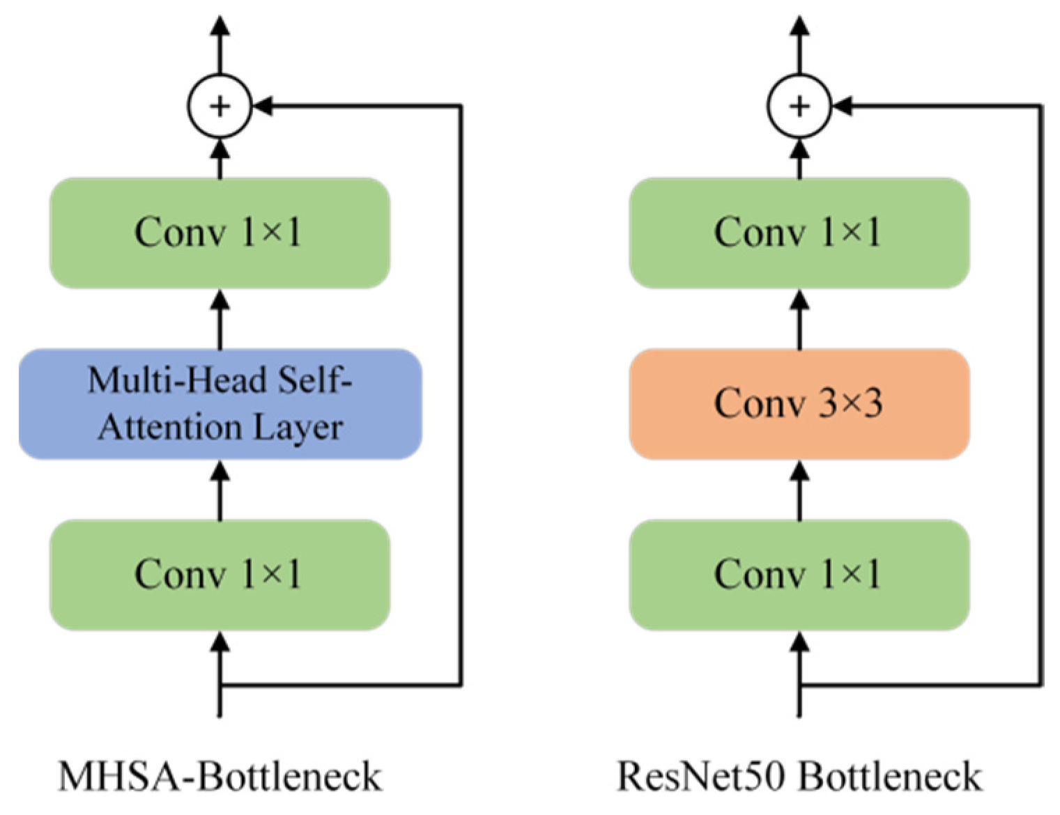
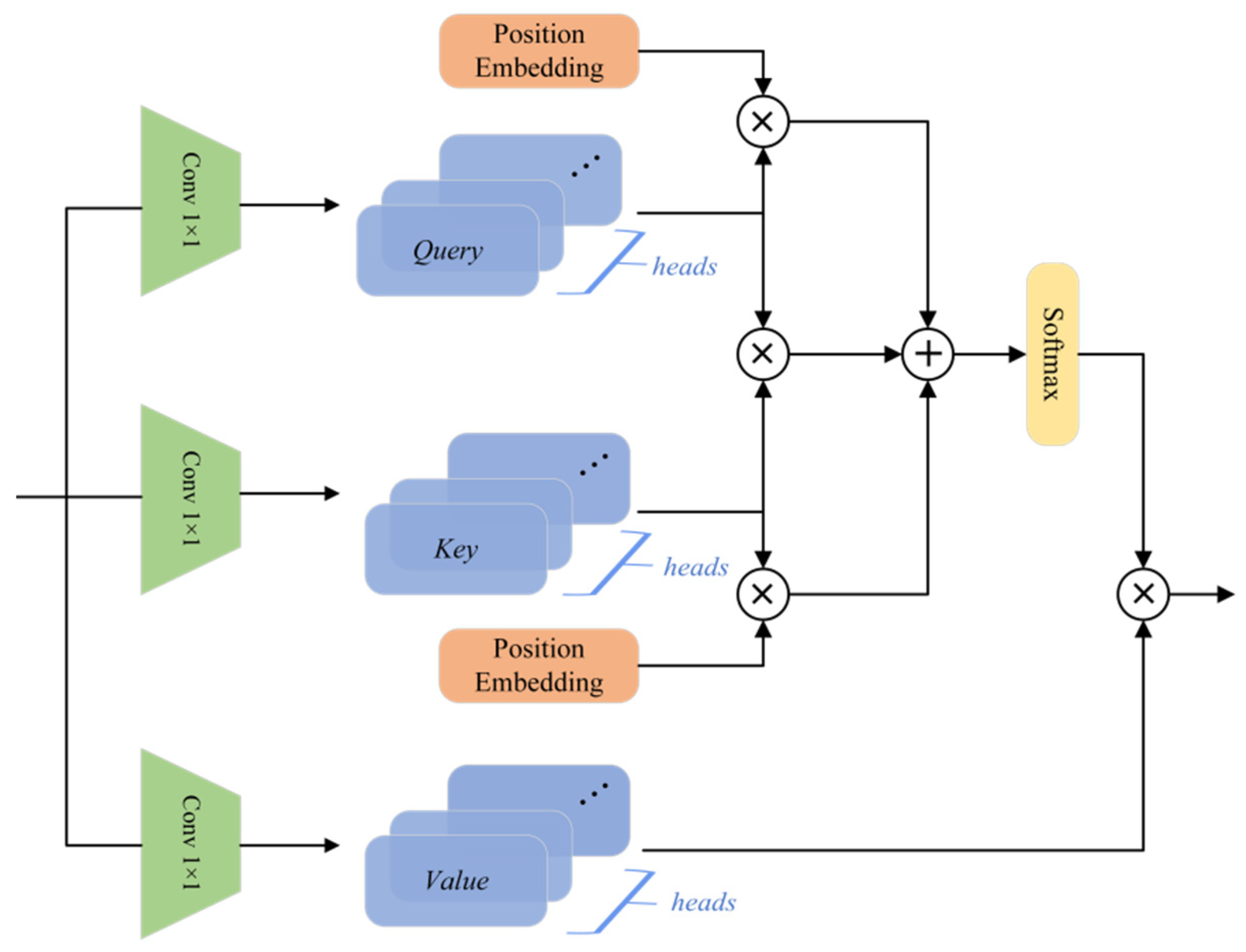
As shown in Figure 3, the MHSA layer was used to replace the 3 × 3 spatial convolutions in the bottleneck. The Transformer can only take a two-dimensional matrix as an input, which ignores the three-dimensional relationships that exist in the matrix. To address this problem, we designed the MHSA-Bottleneck for three-dimensional matrices as an intermediate structure between the CNNs and Transformer encoders. The latest work [70] in the field believes that excessive use of Batch Normalization (BN) [71] will affect the independence of training samples in the batch, so we replaced the BN with Group Normalization [72]. We used the 1 × 1 convolution to obtain the Q, K, and V matrices. We find that the absolute position embedding of Formula (2) does not perform well in the position embedding of a three-dimensional matrix. Therefore, we used the relative position-coding in [18]. The attention calculation formula is shown in (6), and the architecture of the MHSA layer is shown in Figure 4.
A t t e n t i o n ( Q , K , V , P ) = S o f t m a x ( Q P + Q K + K P d ) V ,
where P is the relative position embedding matrix.
We used the MHSA-Bottleneck to replace 6 bottlenecks in ResNet50. We do not replace all bottleneck spatial convolutions with MHSA layers because we found that the performance of self-attention in extracting image edge features and semantic features was not as good as the CNNs in the experiments. The specific experimental results are shown in Section 4.
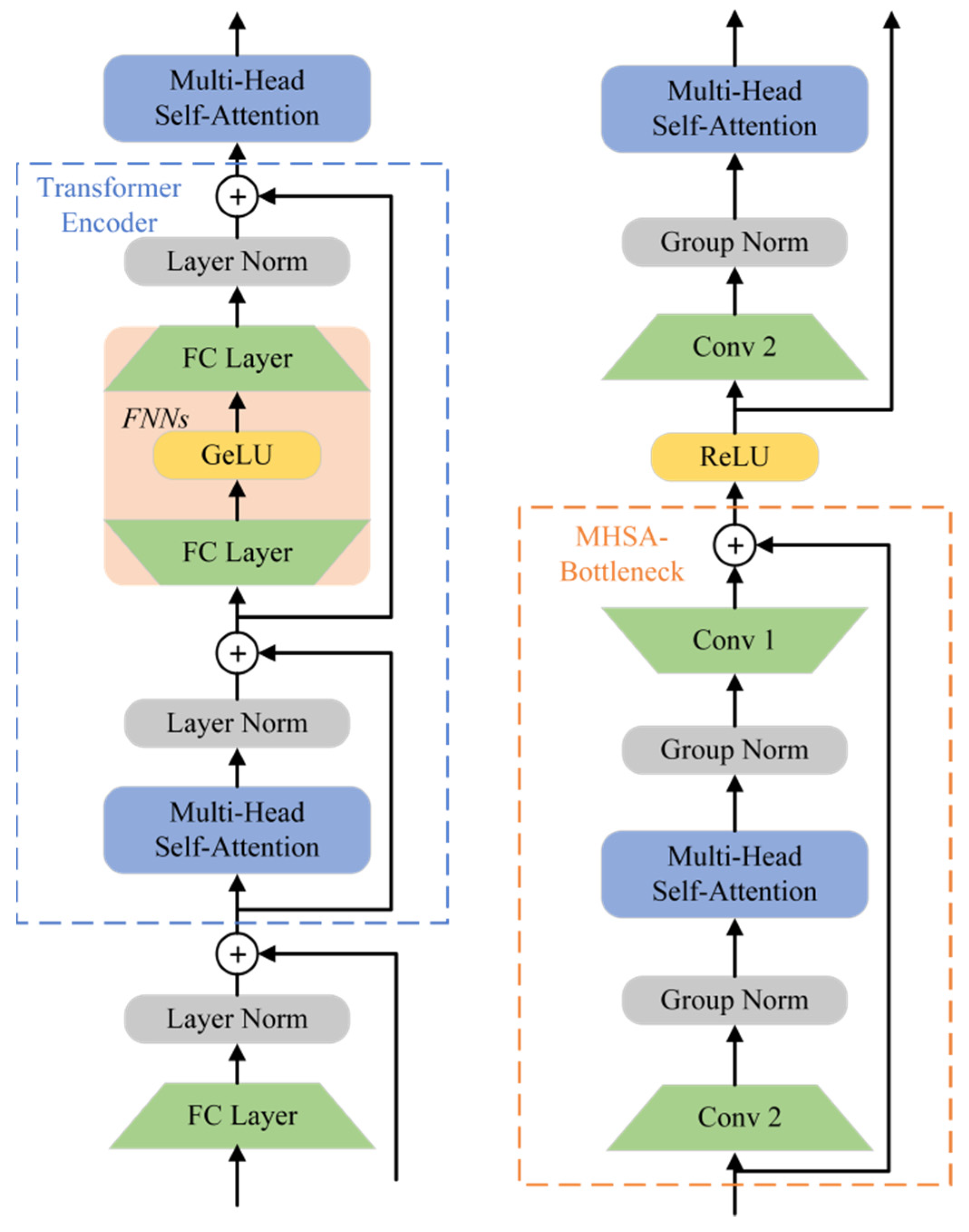
In addition, the relationship between the MHSA-Bottlenecks and Transformers is another important contribution. As shown in Figure 5, we believe that the stacked MHSA-Bottlenecks can be regarded as a Transformer encoder that can process three-dimensional matrices:
(1)
We regard conv1 and conv2 in Figure 5 as FNNs in the Transformer architecture. Both FNNs and convolutional layers were used to increase a certain dimension of the input matrix by 4 times, and then compress it to its original size.
(2)
Both the MHSA-Bottleneck and Transformer architecture used residual connections. The specific differences can be found in Figure 5.
(3)
The Layer Norm was used in the Transformer, and the Group norm was used in the MHSA-Bottleneck.

4. Experiments

In this section, we introduce the datasets, training details, and evaluation protocol used in the experiment. We perform a comprehensive ablation study from three aspects and then provide state-of-the-art comparisons.

4.1. Dataset Description

UC-Merced Dataset: UC-Merced Dataset is one of the most classic datasets in remote sensing scene classification tasks, containing 2100 remote sensing scene images. UC-Merced consists of 21 types of remote sensing scenes. Each type contains 100 pictures, and the resolution of each picture is 256 × 256. UC-Merced was first proposed in [73], and the author used the data again in [74]. The dataset is collected by the U.S. Geological Survey.
Aerial Image Dataset: Aerial Image Dataset (AID) dataset [75] is collected from Google Earth by Wuhan University. AID has a total of 10,000 remote sensing scene images covering 30 remote sensing scene categories, which is a large-scale dataset.
NWPU-RESISC45 Dataset: NWPU-RESISC45 (NWPU) [9] is created by Northwestern Polytechnical University which is a large-scale dataset. NWPU consists of 31,500 images with 256 × 256 pixels. The dataset covers a total of 45 remote sensing scene categories, each with 700 images.
OTIMAL-31 Dataset: OPTIMAL-31 [38] is also collected from Google Earth by Wuhan University. OPTIMAL-31 is a relatively small dataset composed of complex remote sensing scenes. There are 1860 images in total. Each type contains 60 pictures and the resolution of each picture is 256 × 256.

4.2. Training Details

The training equipment we used is shown in Table 2. All experiments are trained for 80 epochs. We used Adam as our optimizer. Since we adopt distributed training on a 4 × NVIDIA TITAN XP GPUs, we set the initial learning rate to 0.0004 (0.0001 × 4), weight decay is 0.00001. We reshape UC-Merced, NWPU, and OPTIMAL-31 into 224 × 224 sizes, and set the batch size to 64. We reshape AID into 600 × 600, and set the batch size to 16. We use 12 Transformer encoders instead of the last three bottlenecks in ResNet50, the number of Multi-Head Self-Attention heads in Transformers is also 12. The number of heads in MHSA-Bottleneck is set to 6, the hyper-parameter λ of absolute position embedding is set to 10,000, and d is set to 384.
For UC-Merced, we set the training ratio to 50% and 80%. For AID, we set the training ratio to 20% and 50%. For NWPU, we set the training ratio to 10% and 20%. For OPTIMAL-31, we set the training ratio to 80%. Training code will be available at: https://github.com/zhangjrjlu/TRS, accessed on 14 October 2021.

4.3. Comparison with CNNs State-of-the-Art

The main purpose of this paper is to demonstrate that optimizing CNNs with Transformers can improve the performance of the network. Therefore, we do not compare TRS with traditional handcrafted features. We use overall accuracy as our evaluation metric, and all results of comparison experiments are obtained from other researchers. At the same time, we only use the ImageNet1K pre-trained parameters in S1, S2 and S3 of the model.
UC-Merced Dataset: The experimental results are shown in Table 3. The “-” in Table 3 means that the model did not complete the experiment under 50% for training or 80% for training. This representation method is applicable to the experimental results of all datasets, and will not be explained hereafter. When the training ratio is 50%, Xu et al. [37] designed lie group features and proposed a new pooling method to improve the training effect, which obtained an accuracy of 98.61 ± 0.11%. Our TRS achieves 98.76 ± 0.23% accuracy, which is 0.15% higher than Xu’s method. When the training ratio is 80%, our method achieves 99.52 ± 0.17% accuracy, which is 0.54% higher than EfficientNet-B3-aux [76] and 0.55% higher than Concourlet CNN [77]. ResNeXt101 + MTL [78] uses multitask learning and achieves an accuracy of 99.11 ± 0.25%, but it is still 0.41% lower than our method. ARCNet + VGGnet16 introduced multi-layer LSTMs and optimized them for the UCMerced dataset to achieve an accuracy of 99.12 ± 0.40%. TRS is 0.40% higher than ARCNet + VGGnet16, which not only proves the effectiveness of our method but also proves that the performance of Transformers is better than LSTMs. The confusion matrices of the results on UC-Merced test set are shown in Figure 6.
Table 3. Classification accuracy on UC-Merced Dataset.
MethodTop1
50% for Training80% for Training
VGGNet [75]94.14 ± 0.6995.21 ± 1.20
GoogleNet [75]92.70 ± 0.6094.31 ± 0.89
D-CNN with AlexNet [75]-97.42 ± 1.79
D-CNN with VGGNet-16 [75]-96.67 ± 0.94
APDCNet [32]95.01 ± 0.4397.05 ± 0.43
SRSCNN [79]97.88 ± 0.3198.13 ± 0.33
EfficientNet-B0-aux [76]98.01 ± 0.45-
EfficientNet-B3-aux [76]98.22 ± 0.49-
MobileNet V2 [80]97.88 ± 0.3198.13 ± 0.33
ResNeXt-101 [81]-98.96 ± 0.31
Contourlet CNN [77]-98.97 ± 0.21
SE-MDPMNet [82]98.57 ± 0.1198.95 ± 0.12
LiG with RBF kernel [83]98.32 ± 0.1398.92 ± 0.35
Xu’s method [37]98.61 ± 0.2298.97 ± 0.31
ResNeXt101-MTL [78]-99.11 ± 0.25
ARCNet-VGGNet16 [38]96.81 ± 0.1499.12 ± 0.40
TRS (ours)98.76 ± 0.1399.52 ± 0.17
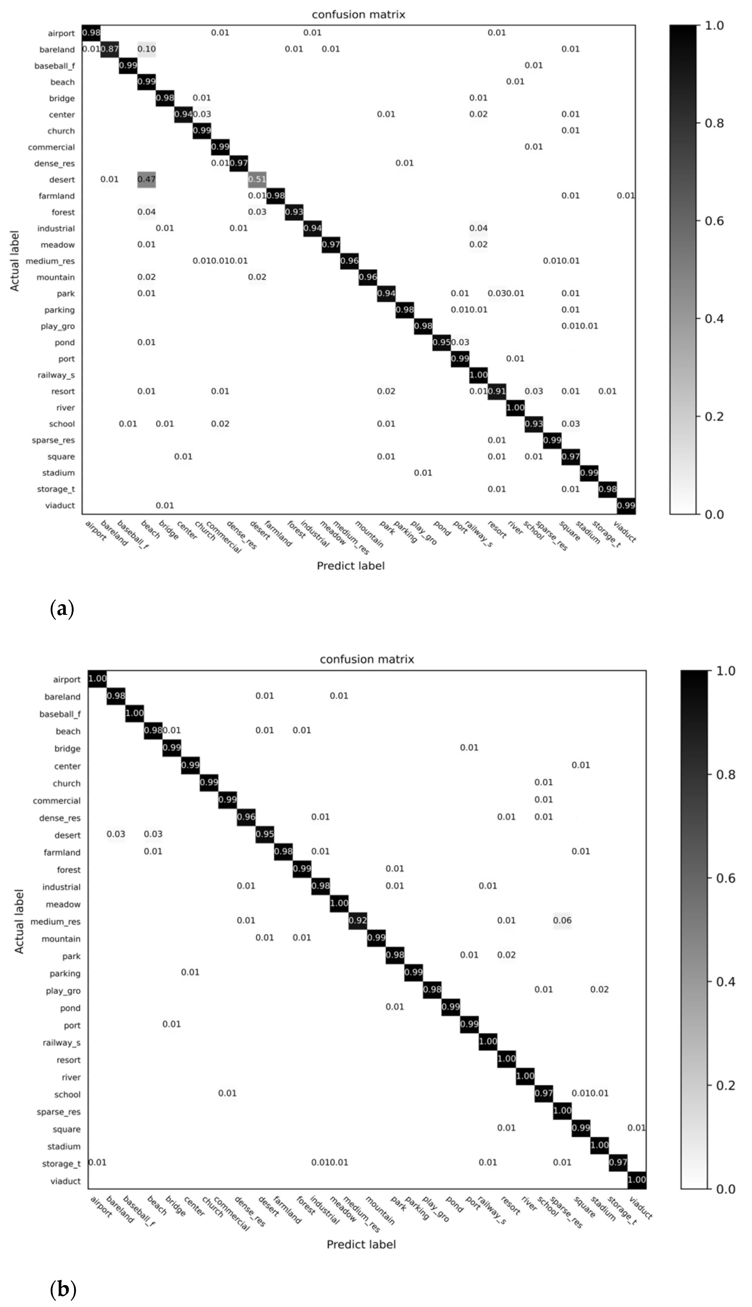
AID Dataset: The image resolution of AID is 600 × 600, which tests the performance of the model more than the UC-Merced dataset. The experimental results are shown in Table 4. At 20% AID training ratios, TRS achieves 95.54 ± 0.18% accuracy, which is 0.8% higher than the second-best Xu’s method [37] and 0.86% higher than SE-MDPMNet [82]. In the case of 50% AID training ratios, our method achieves an accuracy of 98.48 ± 0.06%. TRS is 0.83% higher than Xu’s method, 1.12% higher than Concourlet CNN [76], and 1.34% higher than SE-MDPMNet. The experimental results prove that TRS also has an outstanding ability to understand high-resolution images. The confusion matrices of the results on AID test set are shown in Figure 7. It can be seen from Figure 7a that TRS has low classification accuracy for the “desert” scene. The reason for low accuracy is that TRS regards the part of “desert” as “beach”.
Table 4. Classification accuracy on AID Dataset.
MethodTop1
20% for Training50% for Training
VGGNet [75]86.59 ± 0.2989.64 ± 0.36
GoogleNet [75]83.44 ± 0.4086.39 ± 0.55
SPPNet [75]87.44 ± 0.4591.45 ± 0.38
MobileNet [80]88.53 ± 0.1790.91 ± 0.18
EfficientNet-B0-aux [76]93.96 ± 0.11-
EfficientNet-B3-aux [76]94.19 ± 0.15-
GBNet [36]90.16 ± 0.2493.72 ± 0.34
GBNet + global feature [36]92.20 ± 0.2395.48 ± 0.12
ResNet50 [10]92.39 ± 0.1594.96 ± 0.19
DenseNet-121 [84]93.76 ± 0.2394.73 ± 0.26
MobileNet V2 [80]94.13 ± 0.2895.96 ± 0.27
Contourlet CNN [77]-97.36 ± 0.45
LiG with RBF kernel [83]94.17 ± 0.2596.19 ± 0.28
ResNeXt-101 + MTL [78]93.96 ± 0.1196.89 ± 0.18
SE-MDPMNet [82]94.68 ± 0.0797.14 ± 0.15
Xu’s method [37]94.74 ± 0.2397.65 ± 0.25
TRS (ours)95.54 ± 0.1898.48 ± 0.06
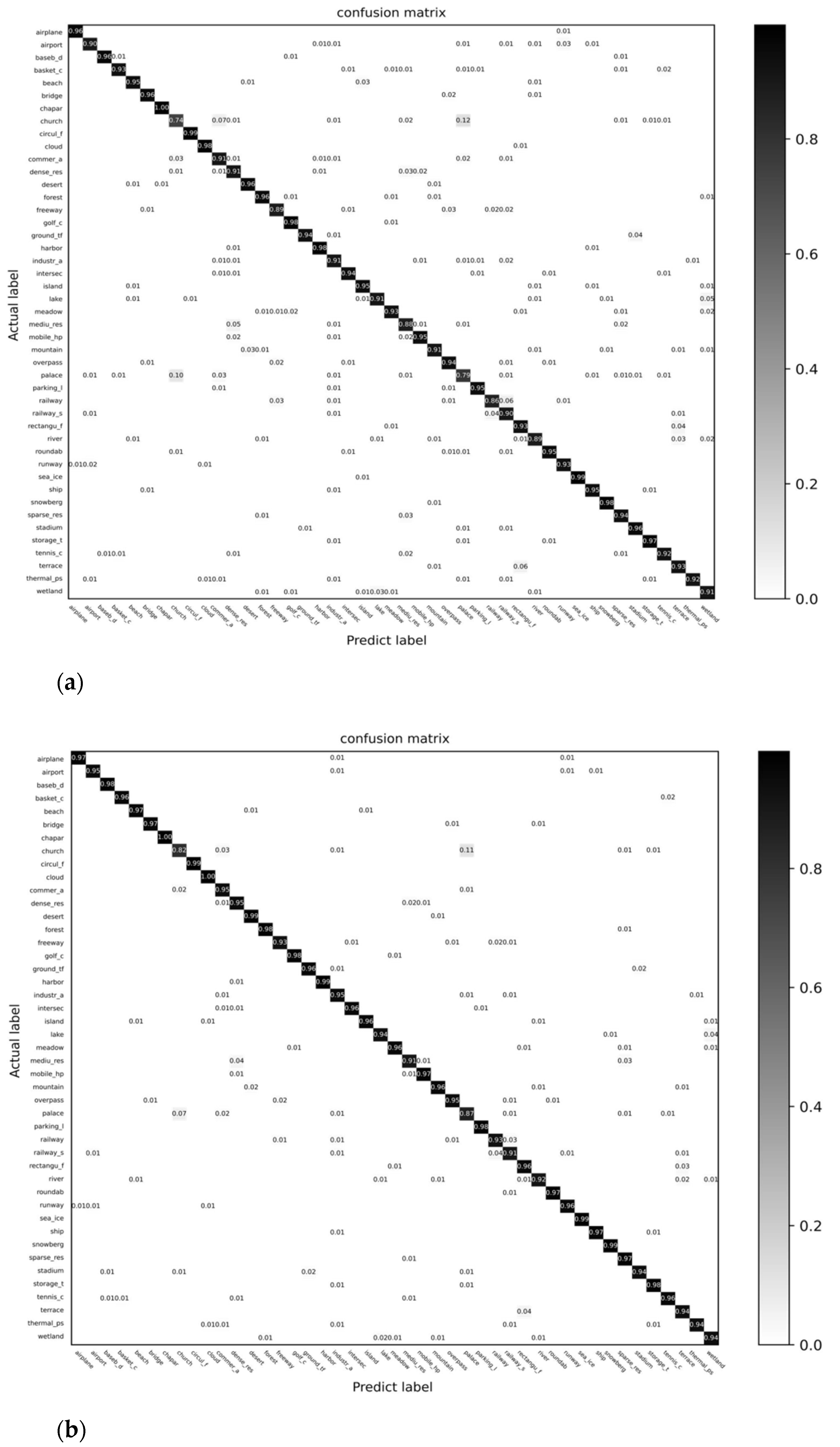
NWPU-RESISC45 Dataset: Compared with AID and UC-Merced, NWPU has more remote sensing scenes and is more difficult to train. The experimental results are shown in Table 5. At 10% NWPU training ratios, TRS achieves 93.06 ± 0.11% accuracy, which is 1.15% higher than Xu’s method and ResNeXt101 + MTL, and 1.26% higher than SE-MDPMNet [82]. In the case of 20% training ratios, TRS achieves an accuracy of 95.56 ± 0.20%, which is 1.13% higher than Xu’s method and 1.35% higher than ResNeXt101 + MTL [78]. The confusion matrices of the results on NWPU test set are shown in Figure 8.
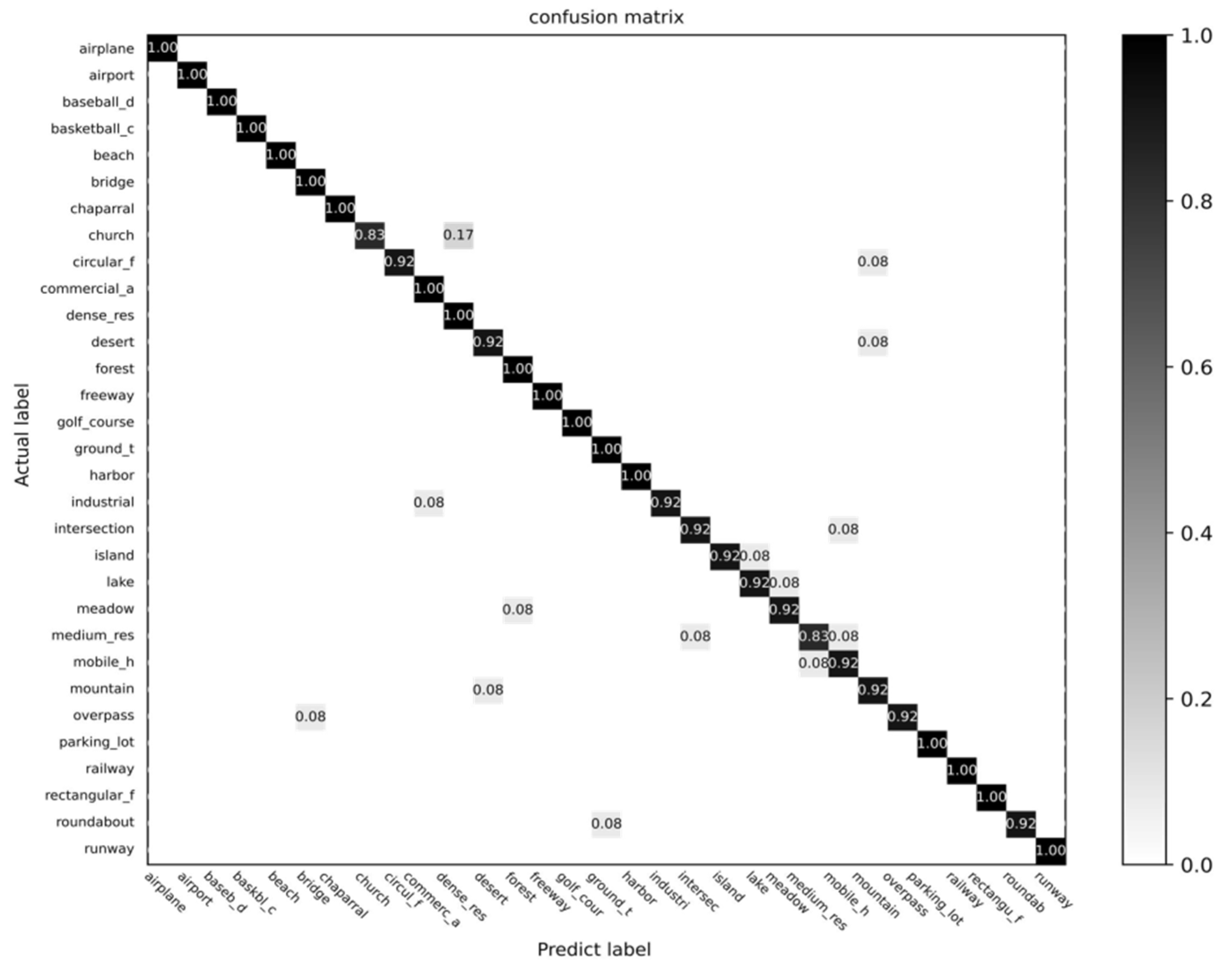
OPTIMAL-31 Dataset: OPTIMAL-31 only contains 60 images for each category, which is a huge challenge for the learning ability and generalization of the model. As shown in Table 6, GBNet [36] integrates different layers of information and achieves 91.40 ± 0.27% with a training ratio of 80%. GBNet achieved an accuracy of 93.28 ± 0.27% after adding the global feature. Our method achieves 95.97 ± 0.13% accuracy. It is 1.88% higher than GBNet + Global feature [36] and 2.46% higher than ARCNet-VGGNet16. The confusion matrix of OPTIMAL-31 is shown in Figure 9.
Table 6. Classification accuracy on OPTIMAL-31 Dataset.
MethodTop1
80% for Training
Fine-tune AlexNet [85]81.22 ± 0.19
Fine-tune VGGNet [85]87.15 ± 0.45
Fine-tune GoogleNet [85]82.57 ± 0.12
ARCNet-ResNet34 [38]91.28 ± 0.45
GBNet [36]91.40 ± 0.27
ARCNet-VGGNet16 [38]92.70 ± 0.35
GBNet + global feature [36]93.28 ± 0.27
EfficientNet-B0-aux [76]93.97 ± 0.12
EfficientNet-B3-aux [76]94.51 ± 0.75
TRS (ours)95.97 ± 0.13

4.4. Comparison with Other Attention Models

In this section, we compare TRS with other models that use attention to optimize ResNet50. As shown in Table 7. Our TRS is 3.52% and 6.65% higher than the standard ResNet50 on AID and NWPU, respectively. Our method is 1.77% and 2.06% higher than ResNeSt, which is known as the best-improved version of ResNet.
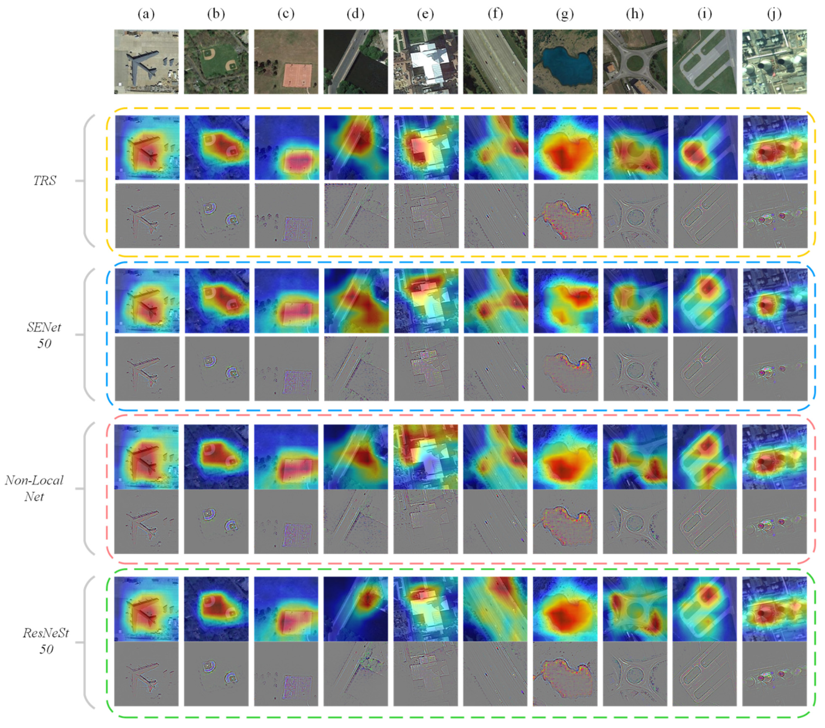
We visualized Class Activation Mapping (CAM) [86] and Guided-Backpropagation (GB) [87]. Interpretability is an important evaluation criterion for deep models. We use Grad-CAM to visualize CAM and GB to prove that TRS is interpretable, and compare the visualized results with SENet [19], Non-local Net [21], and ResNeSt [51]. Class activation mapping shows how each pixel of the image affects the output of the model. Guided-Backpropagation shows the features extracted by the model. We selected 10 remote sensing scene classes: (a) Airplane, (b) Baseball diamond, (c) Basketball court, (d) Bridge, (e) Church, (f) Freeway, (g) Lake, (h) Roundabout, (i) Runway, (j) Thermal power station. The experimental results shown in Figure 10 demonstrate that TRS has more powerful performance than several other attention models. The experimental results also explain why TRS has higher remote sensing scene classification accuracy from the perspective of interpretability.

4.5. Comparison with Other Transformers

We also compared the TRS with other Transformers. The experimental results are shown in Table 8 and Table 9. TRS has obvious advantages over other excellent Transformers. The experimental results show that the ViT [23] based on global attention does not show strong performance for remote sensing scene classification, but the ViT-Hybrid [23] does well. The Swin Transformer [63] uses windows to complete local and global attention, and achieves better results than CNNs. However, the TRS achieves higher accuracy than the Swin Transformer. For the experiments of these Transformers, our code was based on the Timm package (https://github.com/rwightman/pytorch-image-models, accessed on 14 October 2021), and we used the ImageNet1k pretrained model.

4.6. Training, Testing Time and Parameters

Training and testing time can intuitively reflect the efficiency of the model. Acc. in the table refers to overall accuracy, and FLOPs refer to floating-point operations. All experiments are performed on an NVIDIA GTX 2080Ti GPU. To compare the time it takes to train and test each model for an epoch, we use tqdm package. As shown in Table 10, the time it takes for TRS to train and test an epoch is very close to ResNet-101, nevertheless, the former’s accuracy is higher than the latter. Compared with models whose accuracy is close to ours, the training and testing time of Swin-Base are 5 seconds and 0.9 seconds slower than TRS, respectively; the training and testing times of ViT-Hybrid are 6.9 seconds and 2.9 seconds lower than our model. We also show the parameters and FLOPs of the models. The weight parameters and FLOPs of TRS are 46.3M and 8.4G, respectively, which surpass ResNet-101 by only 0.3M and 0.8G, respectively. However, the weight parameters and FLOPs of TRS decrease by 41.7M and 7G compared with Swin-Base, which ranks second in accuracy.

5. Discussion

5.1. Ablation Study

In the ablation study, we explored how the components of the TRS affect the performance of the model. In order to obtain more convincing results, we chose to conduct ablation experiments on two datasets with different resolutions, AID and NWPU. The training ratios of AID and NWPU were 50% and 20%, respectively.

5.1.1. Number of Encoder Layers and Self-Attention Heads

We changed the number of encoder layers and self-attention heads to evaluate the importance of the Transformer architecture. The experimental results are shown in Table 11. When there was no encoder layer, we used the GlobalAvgPooling to process the output of Stage3 (S3) in Table 1, and used the fully connected layer for scene classification. We found that the classification accuracy on AID and NWPU decreased by 7.01% and 9.26%, respectively, without the Transformer encoder. When using three encoder layers, the accuracy of the TRS was 0.67% and 1.66% higher than ResNet50, respectively. TRS achieves the best accuracy when the number of Transformer encoders is 12. At the same time, TRS achieves the best accuracy when the number of Multi-Head Self-Attention heads is 12. The experimental results show that the Transformer architecture is effective in remote sensing scene classification.

5.1.2. MHSA-Bottleneck Architecture

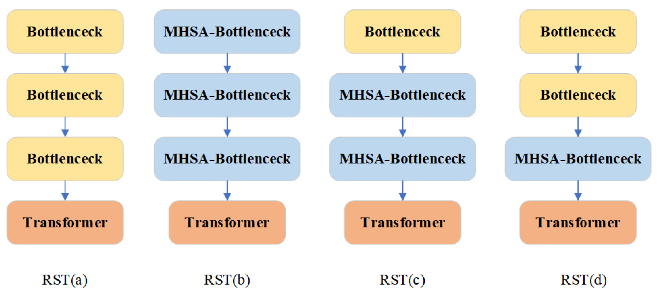
We also conducted an ablation study on the arrangement of the MHSA-Bottleneck in the TRS. For comparison, several structures are shown in Figure 11, and the experimental results are shown in Table 12. The accuracy of the TRS (a) was 2.28% and 3.61% lower than TRS (d), respectively. The results demonstrate the importance of using our proposed MHSA-Bottleneck as an intermediate structure between CNNs and Transformer encoders. In TRS (b), all bottlenecks were replaced by the MHSA-Bottleneck, the accuracy was lower than TRS (a). This shows that relying only on self-attention to learn the relationship between features cannot achieve good results, and the combination of CNNs’ feature extraction ability and self-attention has better performance. We also test the number of self-attention heads and standardized methods of the MHSA-Bottleneck. The experimental results are shown in Table 13.

5.1.3. Position Embedding

There are two ways of our position embedding: absolute position embedding and relative position embedding. We tried a combination of these two encoding methods, and the results of the experiment are shown in Table 14. Without position embedding, the accuracy of TRS is 4.52% and 2.33% lower than the ResNet50, respectively. Therefore, position embedding is required. The accuracy of using relative position embedding or absolute position embedding in Transformers is almost the same, while the accuracy of using relative position embedding in MHSA-Bottleneck is higher than that of absolute position embedding.
Given these ablation experiments, we came to the conclusion: Transformer encoders, MHSA-Bottlenecks, and position embedding all contributed to the performance of TRS.

5.2. Application Scenarios

A transformer is a great way to learn Global information which is the current development trend of remote sensing image tasks. However, the current work believes that local information must be combined to obtain better results. Our proposed model uses CNNs to extract Local information and uses Transformer to extract Global information. Through the results of Table 10, we can get a conclusion: the parameters of the existing models are redundant for remote sensing scene classification tasks, and there is no need to make the model larger to improve the performance. We believe that using a limited number of parameters to obtain better performance is a better solution to improve the classification effect of remote sensing scenes, and TRS has outstanding performance in this regard.
At the same time, our model can not only be used for remote sensing scene classification, but also provide rich features for downstream tasks. Downstream tasks can obtain image features at different resolutions as the input of FPN [88], and the current method of applying Transformer to remote sensing scene classification cannot do this well, such as [25,57,89]. We can input the features extracted from TRS S2-S5 into FPN to complete downstream tasks.

6. Conclusions

In this paper, we proposed the TRS, a new design for remote sensing scene classification based on the Transformer. We successfully used the Transformer for remote sensing scene classification for the first time, and proposed a novel "pure CNNs → Convolution + Transformer → pure Transformers" structure. We designed the MHSA-Bottleneck and proposed to replace spatial convolution with the Multi-Head Self-Attention. At the same time, we provided a new idea to understand MHSA-Bottleneck as a Transformer that processes three-dimensional matrices. We also replaced the bottleneck with multiple standard Transformer encoders. The experimental results of the four public datasets demonstrate that the TRS is robust, surpasses previous work, and achieves state-of-the-art.
We hope that we can not only apply the Transformer encoder to remote sensing scene classification, but also that the transformer decoder and transformer encoder can be combined and applied to other remote sensing tasks. In further works, we will attempt to apply the complete Transformer architecture (encoder + decoder) to remote sensing tasks.

Author Contributions

J.Z. and J.L. completed the investigation. J.Z. and H.Z. designed and implemented the method, and wrote the paper. J.L. and H.Z. contributed to the analysis of the experimental results All authors have read and agreed to the published version of the manuscript.

Funding

This research was funded by the Provincial Science and Technology Innovation Special Fund Project of Jilin Province, grant number 20190302026GX, Natural Science Foundation of Jilin Province, grant number 20200201037JC.

Data Availability Statement

Data sharing is not applicable to this article.

Conflicts of Interest

The authors declare no conflict of interest.

References

  1. Chen, M.; Liu, D.; Qian, K.; Li, J.; Lei, M.; Zhou, Y. Lunar crater detection based on terrain analysis and mathematical morphology methods using digital elevation models. IEEE Trans. Geosci. Remote Sens. 2018, 56, 3681–3692. [Google Scholar] [CrossRef]
  2. Ye, F.; Xiao, H.; Zhao, X.; Dong, M.; Luo, W.; Min, W. Remote sensing image retrieval using convolutional neural network features and weighted distance. IEEE Geosci. Remote Sens. Lett. 2018, 15, 1535–1539. [Google Scholar] [CrossRef]
  3. Li, J.; Benediktsson, J.A.; Zhang, B.; Yang, T.; Plaza, A. Spatial technology and social media in remote sensing: A survey. Proc. IEEE 2017, 105, 1855–1864. [Google Scholar] [CrossRef]
  4. Luo, F.; Huang, H.; Duan, Y.; Liu, J.; Liao, Y. Local geometric structure feature for dimensionality reduction of hyperspectral imagery. Remote Sens. 2017, 9, 790. [Google Scholar] [CrossRef] [Green Version]
  5. Lowe, D.G. Distinctive image features from scale-invariant keypoints. Int. J. Comput. Vis. 2004, 60, 91–110. [Google Scholar] [CrossRef]
  6. Ojala, T.; Pietikainen, M.; Maenpaa, T. Multiresolution gray-scale and rotation invariant texture classification with local binary patterns. IEEE Trans. Pattern Anal. Mach. Intell. 2002, 24, 971–987. [Google Scholar] [CrossRef]
  7. Wang, G.; Fan, B.; Xiang, S.; Pan, C. Aggregating rich hierarchical features for scene classification in remote sensing imagery. IEEE J. Sel. Top. Appl. Earth Observ. Remote Sens. 2017, 10, 4104–4115. [Google Scholar] [CrossRef]
  8. Yang, S.; Ramanan, D. Multi-scale recognition with DAG-CNNs. In Proceedings of the IEEE International Conference on Computer Vision, Washington, DC, USA, 7–13 December 2015; pp. 1215–1223. [Google Scholar]
  9. Simonyan, K.; Zisserman, A. Very deep convolutional networks for large-scale image recognition. In Proceedings of the ICLR 2015: International Conference on Learning Representations, San Diego, CA, USA, 7–9 May 2015. [Google Scholar]
  10. He, K.; Zhang, X.; Ren, S.; Sun, J. Deep residual learning for image recognition. In Proceedings of the IEEE Conference on Computer Vision and Pattern Recognition, Las Vegas, NV, USA, 27–30 June 2016; pp. 770–778. [Google Scholar]
  11. Liang, Y.; Monteiro, S.T.; Saber, E.S. Transfer learning for high resolution aerial image classification. In Proceedings of the 2016 IEEE Applied Imagery Pattern Recognition Workshop (AIPR), Washington, DC, USA, 18–20 October 2016; pp. 1–8. [Google Scholar]
  12. Vaswani, A.; Shazeer, N.; Parmar, N.; Uszkoreit, J.; Jones, L.; Gomez, A.N.; Kaiser, Ł.; Polosukhin, I. Attention is all you need. In Proceedings of the Advances in Neural Information Processing Systems, Long Beach, CA, USA, 4–9 December 2021; pp. 5998–6008. [Google Scholar]
  13. Radford, A.; Wu, J.; Child, R.; Luan, D.; Amodei, D.; Sutskever, I. Language models are unsupervised multitask learners. OpenAI Blog 2019, 1, 9. [Google Scholar]
  14. Brown, T.B.; Mann, B.; Ryder, N.; Subbiah, M.; Kaplan, J.; Dhariwal, P.; Askell, A. Language models are few-shot learners. In Advances in Neural Information Processing Systems; MIT Press: Cambridge, MA, USA, 2020; Volume 33, pp. 1877–1901. [Google Scholar]
  15. Devlin, J.; Chang, M.-W.; Lee, K.; Toutanova, K.N. Bert: Pre-training of deep bidirectional transformers for language understanding. In Proceedings of the 2019 Conference of the North American Chapter of the Association for Computational Linguistics: Human Language Technologies, New Orleans, LA, USA, 1–6 June 2018; Volume 1, pp. 4171–4186. [Google Scholar]
  16. Liu, Y.; Ott, M.; Goyal, N.; Du, J.; Joshi, M.; Chen, D.; Stoyanov, V. Roberta: A robustly optimized bert pretraining approach. arXiv 2019, arXiv:1907.11692. [Google Scholar]
  17. Wang, H.; Zhu, Y.; Green, B.; Adam, H.; Yuille, A.L.; Chen, L.-C. Axial-deeplab: Stand-alone axial-attention for panoptic segmentation. In Proceedings of the European Conference on Computer Vision, Glasgow, UK, 23–28 August 2020; pp. 108–126. [Google Scholar]
  18. Ramachandran, P.; Parmar, N.; Vaswani, A.; Bello, I.; Levskaya, A.; Shlens, J. Stand-alone self-attention in vision models. In Proceedings of the Advances in Neural Information Processing Systems, Vancouver, BC, Canada, 8–14 December 2019; Volume 32, pp. 68–80. [Google Scholar]
  19. Hu, J.; Shen, L.; Sun, G. Squeeze-and-excitation networks. In Proceedings of the IEEE Conference on Computer Vision and Pattern Recognition, Salt Lake City, UT, USA, 18–22 June 2018; pp. 7132–7141. [Google Scholar]
  20. Woo, S.; Park, J.; Lee, J.Y.; Kweon, I.S. Cbam: Convolutional block attention module. In Proceedings of the European Conference on Computer Vision (ECCV), Munich, Germany, 8–14 September 2018; pp. 3–19. [Google Scholar]
  21. Li, X.; Wang, W.; Hu, X.; Yang, J. Selective kernel networks. In Proceedings of the IEEE/CVF Conference on Computer Vision and Pattern Recognition, Long Beach, CA, USA, 15–20 June 2019; pp. 510–519. [Google Scholar]
  22. Wang, X.; Girshick, R.; Gupta, A.; He, K. Non-local neural networks. In Proceedings of the IEEE Conference on Computer Vision and Pattern Recognition, Salt Lake City, UT, USA, 18–22 June 2018; pp. 7794–7803. [Google Scholar]
  23. Dosovitskiy, A.; Beyer, L.; Kolesnikov, A.; Weissenborn, D.; Zhai, X.; Unterthiner, T.; Gelly, S. An image is worth 16 × 16 words: Transformers for image recognition at scale. In Proceedings of the ICLR 2021: The Ninth International Conference on Learning Representations, Virtual Event, 3–7 May 2021. [Google Scholar]
  24. Yuan, L.; Chen, Y.; Wang, T.; Yu, W.; Shi, Y.; Jiang, Z.; Yan, S. Tokens-to-token vit: Training vision transformers from scratch on imagenet. arXiv 2021, arXiv:2101.11986. [Google Scholar]
  25. Carion, N.; Massa, F.; Synnaeve, G.; Usunier, N.; Kirillov, A.; Zagoruyko, S. End-to-end object detection with transformers. In Proceedings of the European Conference on Computer Vision, Glasgow, UK, 23–28 August 2020; pp. 213–229. [Google Scholar]
  26. Wang, W.; Xie, E.; Li, X.; Fan, D.P.; Song, K.; Liang, D.; Shao, L. Pyramid vision transformer: A versatile backbone for dense prediction without convolutions. arXiv 2021, arXiv:2102.12122. [Google Scholar]
  27. Krizhevsky, A.; Sutskever, I.; Hinton, G.E. Imagenet classification with deep convolutional neural networks. Adv. Neural Inf. Process. Syst. 2012, 25, 1097–1105. [Google Scholar] [CrossRef]
  28. Cheng, G.; Han, J.; Lu, X. Remote sensing image scene classification: Benchmark and state of the art. Proc. IEEE 2017, 105, 1865–1883. [Google Scholar] [CrossRef] [Green Version]
  29. Szegedy, C.; Liu, W.; Jia, Y.; Sermanet, P.; Reed, S.; Anguelov, D.; Rabinovich, A. Going deeper with convolutions. In Proceedings of the IEEE Conference on Computer Vision and Pattern Recognition, Boston, MA, USA, 7–12 June 2015; pp. 1–9. [Google Scholar]
  30. Yu, Y.; Liu, F. Aerial scene classification via multilevel fusion based on deep convolutional neural networks. IEEE Geosci. Remote Sens. Lett. 2018, 15, 287–291. [Google Scholar] [CrossRef]
  31. Tan, M.; Le, Q. Efficientnet: Rethinking model scaling for convolutional neural networks. In Proceedings of the International Conference on Machine Learning, Crete, Greece, 24–26 May 2019; pp. 6105–6114. [Google Scholar]
  32. Bi, Q.; Qin, K.; Zhang, H.; Xie, J.; Li, Z.; Xu, K. APDC-Net: Attention pooling-based convolutional network for aerial scene classification. IEEE Geosci. Remote Sens. Lett. 2019, 17, 1603–1607. [Google Scholar] [CrossRef]
  33. Hu, F.; Xia, G.S.; Hu, J.; Zhang, L. Transferring deep convolutional neural networks for the scene classification of high-resolution remote sensing imagery. Remote Sens. 2015, 7, 14680–14707. [Google Scholar] [CrossRef] [Green Version]
  34. Li, E.; Xia, J.; Du, P.; Lin, C.; Samat, A. Integrating multilayer features of convolutional neural networks for remote sensing scene classification. IEEE Trans. Geosci. Remote Sens. 2017, 55, 5653–5665. [Google Scholar] [CrossRef]
  35. Zhang, F.; Du, B.; Zhang, L. Scene classification via a gradient boosting random convolutional network framework. IEEE Trans. Geosci. Remote Sens. 2015, 54, 1793–1802. [Google Scholar] [CrossRef]
  36. Sun, H.; Li, S.; Zheng, X.; Lu, X. Remote sensing scene classification by gated bidirectional network. IEEE Trans. Geosci. Remote Sens. 2019, 58, 82–96. [Google Scholar] [CrossRef]
  37. Xu, C.; Zhu, G.; Shu, J. A Lightweight and Robust Lie Group-Convolutional Neural Networks Joint Representation for Remote Sensing Scene Classification. IEEE Trans. Geosci. Remote Sens. 2021, 1–15. [Google Scholar] [CrossRef]
  38. Wang, Q.; Liu, S.; Chanussot, J.; Li, X. Scene classification with recurrent attention of VHR remote sensing images. IEEE Trans. Geosci. Remote Sens. 2018, 57, 1155–1167. [Google Scholar] [CrossRef]
  39. Yu, Y.; Li, X.; Liu, F. Attention GANs: Unsupervised deep feature learning for aerial scene classification. IEEE Trans. Geosci. Remote Sens. 2019, 58, 519–531. [Google Scholar] [CrossRef]
  40. Cortes, C.; Vapnik, V. Support vector machine. Mach. Learn. 1995, 20, 273–297. [Google Scholar] [CrossRef]
  41. Joachims, T. Transductive inference for text classification using support vector machines. In Proceedings of the International Conference on Machine Learning (ICML), Bled, Slovenia, 27–30 June 1999; Volume 99, pp. 200–209. [Google Scholar]
  42. Gómez-Chova, L.; Camps-Valls, G.; Munoz-Mari, J.; Calpe, J. Semisupervised image classification with Laplacian support vector machines. IEEE Geosci. Remote Sens. Lett. 2008, 5, 336–340. [Google Scholar] [CrossRef]
  43. Ma, B. A new kind of parallel K_NN network public opinion classification algorithm based on Hadoop platform. Appl. Mech. Mater. 2014, 644, 2018–2021. [Google Scholar]
  44. La, L.; Guo, Q.; Yang, D.; Cao, Q. Multiclass Boosting with Adaptive Group-Based kNN and Its Application in Text Categorization. Math. Probl. Eng. 2012, 2012, 1–24. [Google Scholar] [CrossRef]
  45. Zhu, Q.; Zhong, Y.; Zhao, B.; Xia, G.S.; Zhang, L. Bag-of-visual-words scene classifier with local and global features for high spatial resolution remote sensing imagery. IEEE Trans. Geosci. Remote Sens. Lett. 2016, 13, 747–751. [Google Scholar] [CrossRef]
  46. Yao, W.; Loffeld, O.; Datcu, M. Application and evaluation of a hierarchical patch clustering method for remote sensing images. IEEE J. Sel. Top. Appl. Earth Observ. Remote Sens. 2016, 9, 2279–2289. [Google Scholar] [CrossRef]
  47. Zhao, B.; Zhong, Y.; Zhang, L. A spectral–structural bag-of-features scene classifier for very high spatial resolution remote sensing imagery. ISPRS J. Photogram. Remote Sens. 2016, 116, 73–85. [Google Scholar] [CrossRef]
  48. Zhao, L.; Tang, P.; Huo, L. Feature significance-based multibag-of-visual-words model for remote sensing image scene classification. J. Appl. Remote Sens. 2016, 10, 035004. [Google Scholar] [CrossRef]
  49. Wu, H.; Liu, B.; Su, W.; Zhang, W.; Sun, J. Hierarchical coding vectors for scene level land-use classification. Remote Sens. 2016, 8, 436. [Google Scholar] [CrossRef] [Green Version]
  50. Li, Y.; Tao, C.; Tan, Y.; Shang, K.; Tian, J. Unsupervised multilayer feature learning for satellite image scene classification. IEEE Trans. Geosci. Remote Sens. Lett. 2016, 13, 157–161. [Google Scholar] [CrossRef]
  51. Zhang, H.; Wu, C.; Zhang, Z.; Zhu, Y.; Lin, H.; Zhang, Z.; Smola, A. Resnest: Split-attention networks. arXiv 2020, arXiv:2004.08955. [Google Scholar]
  52. Romera-Paredes, B.; Torr, P.H.S. Recurrent instance segmentation. In Proceedings of the European Conference on Computer Vision, Amsterdam, The Netherlands, 11–14 October 2016; pp. 312–329. [Google Scholar]
  53. Olah, C. Understanding LSTM Networks. Available online: http://colah.github.io/posts/2015-08-Understanding-LSTMs (accessed on 1 October 2015).
  54. Cho, K.; van Merrienboer, B.; Gulcehre, C.; Bahdanau, D.; Bougares, F.; Schwenk, H.; Bengio, Y. Learning Phrase Representations using RNN Encoder--Decoder for Statistical Machine Translation. In Proceedings of the 2014 Conference on Empirical Methods in Natural Language Processing (EMNLP), Doha, Qatar, 25–29 October 2014; pp. 1724–1734. [Google Scholar]
  55. Stewart, R.; Andriluka, M.; Ng, A.Y. End-to-end people detection in crowded scenes. In Proceedings of the IEEE Conference on Computer Vision and Pattern Recognition, Las Vegas, NV, USA, 27–30 June 2016; pp. 2325–2333. [Google Scholar]
  56. Parmar, N.; Vaswani, A.; Uszkoreit, J.; Kaiser, L.; Shazeer, N.; Ku, A.; Tran, D. Image transformer. In Proceedings of the International Conference on Machine Learning, Stockholm, Sweden, 10–15 July 2018; pp. 4055–4064. [Google Scholar]
  57. Child, R.; Gray, S.; Radford, A.; Sutskever, I. Generating long sequences with sparse transformers. arXiv 2019, arXiv:1904.10509. [Google Scholar]
  58. Zhu, X.; Su, W.; Lu, L.; Li, B.; Wang, X.; Dai, J. Deformable DETR: Deformable Transformers for End-to-End Object Detection. In Proceedings of the ICLR 2021: The Ninth International Conference on Learning Representations, Virtual Event, 3–7 May 2021. [Google Scholar]
  59. Bello, I.; Zoph, B.; Vaswani, A.; Shlens, J.; Le, Q.V. Attention augmented convolutional networks. In Proceedings of the IEEE/CVF International Conference on Computer Vision, Seoul, Korea, 27–28 October 2019; pp. 3286–3295. [Google Scholar]
  60. Touvron, H.; Cord, M.; Douze, M.; Massa, F.; Sablayrolles, A.; Jégou, H. Training data-efficient image transformers & distillation through attention. In Proceedings of the International Conference on Machine Learning, Virtual Event, 18–24 July 2021; pp. 10347–10357. [Google Scholar]
  61. Hinton, G.; Vinyals, O.; Dean, J. Distilling the knowledge in a neural network. arXiv 2015, arXiv:1503.02531. [Google Scholar]
  62. Abnar, S.; Dehghani, M.; Zuidema, W. Transferring inductive biases through knowledge distillation. arXiv 2020, arXiv:2006.00555. [Google Scholar]
  63. Liu, Z.; Lin, Y.; Cao, Y.; Hu, H.; Wei, Y.; Zhang, Z.; Guo, B. Swin transformer: Hierarchical vision transformer using shifted windows. arXiv 2021, arXiv:2103.14030. [Google Scholar]
  64. Li, W.; Cao, D.; Peng, Y.; Yang, C. MSNet: A Multi-Stream Fusion Network for Remote Sensing Spatiotemporal Fusion Based on Transformer and Convolution. Remote Sens. 2021, 13, 3724. [Google Scholar] [CrossRef]
  65. Bazi, Y.; Bashmal, L.; Rahhal, M.M.A.; Dayil, R.A.; Ajlan, N.A. Vision Transformers for Remote Sensing Image Classification. Remote Sens. 2021, 13, 516. [Google Scholar] [CrossRef]
  66. Xu, Z.; Zhang, W.; Zhang, T.; Yang, Z.; Li, J. Efficient Transformer for Remote Sensing Image Segmentation. Remote Sens. 2021, 13, 3585. [Google Scholar] [CrossRef]
  67. Hendrycks, D.; Gimpel, K. Gaussian error linear units (gelus). arXiv 2016, arXiv:1606.08415. [Google Scholar]
  68. Nair, V.; Hinton, G.E. Rectified linear units improve restricted boltzmann machines. In Proceedings of the 27th International Conference on Machine Learning, Haifa, Israel, 21–24 June 2010; pp. 807–814. [Google Scholar]
  69. Ba, J.L.; Kiros, J.R.; Hinton, G.E. Layer normalization. arXiv 2016, arXiv:1607.06450. [Google Scholar]
  70. Brock, A.; De, S.; Smith, S.L. Characterizing signal propagation to close the performance gap in unnormalized ResNets. In Proceedings of the ICLR 2021: The Ninth International Conference on Learning Representations, Virtual Event, 3–7 May 2021. [Google Scholar]
  71. Ioffe, S.; Szegedy, C. Batch normalization: Accelerating deep network training by reducing internal covariate shift. In Proceedings of the International Conference on Machine Learning, Lille, France, 6–11 July 2015; pp. 448–456. [Google Scholar]
  72. Wu, Y.; He, K. Group normalization. In Proceedings of the European Conference on Computer Vision (ECCV), Munich, Germany, 8–14 September 2018; pp. 3–19. [Google Scholar]
  73. Yang, Y.; Newsam, S. Geographic image retrieval using local invariant features. IEEE Trans. Geosci. Remote Sens. 2012, 51, 818–832. [Google Scholar] [CrossRef]
  74. Zhang, R.; Isola, P.; Efros, A.A. Colorful image colorization. In Proceedings of the European Conference on Computer Vision, Amsterdam, The Netherlands, 11–14 October 2016; pp. 649–666. [Google Scholar]
  75. Xia, G.S.; Hu, J.; Hu, F.; Shi, B.; Bai, X.; Zhong, Y.; Lu, X. AID: A benchmark data set for performance evaluation of aerial scene classification. IEEE Trans. Geosci. Remote Sens. 2017, 55, 3965–3981. [Google Scholar] [CrossRef] [Green Version]
  76. Bazi, Y.; Al Rahhal, M.M.; Alhichri, H.; Alajlan, N. Simple yet effective fine-tuning of deep CNNs using an auxiliary classification loss for remote sensing scene classification. Remote Sens. 2019, 11, 2908. [Google Scholar] [CrossRef] [Green Version]
  77. Liu, M.; Jiao, L.; Liu, X.; Li, L.; Liu, F.; Yang, S. C-CNN: Contourlet convolutional neural networks. IEEE Trans. Neural Netw. Learn. Syst. 2020, 32, 2636–2649. [Google Scholar] [CrossRef]
  78. Zhao, Z.; Luo, Z.; Li, J.; Chen, C.; Piao, Y. When self-supervised learning meets scene classification: Remote sensing scene classification based on a multitask learning framework. Remote Sens. 2020, 12, 3276. [Google Scholar] [CrossRef]
  79. Liu, Y.; Zhong, Y.; Fei, F.; Zhu, Q.; Qin, Q. Scene classification based on a deep random-scale stretched convolutional neural network. Remote Sens. 2018, 10, 444. [Google Scholar] [CrossRef] [Green Version]
  80. Pan, H.; Pang, Z.; Wang, Y.; Wang, Y.; Chen, L. A new image recognition and classification method combining transfer learning algorithm and mobilenet model for welding defects. IEEE Access 2020, 8, 119951–119960. [Google Scholar] [CrossRef]
  81. Xie, S.; Girshick, R.; Dollár, P.; Tu, Z.; He, K. Aggregated residual transformations for deep neural networks. In Proceedings of the IEEE Conference on Computer Vision and Pattern Recognition, Honolulu, HI, USA, 22–25 July 2017; pp. 1492–1500. [Google Scholar]
  82. Zhang, B.; Zhang, Y.; Wang, S. A lightweight and discriminative model for remote sensing scene classification with multidilation pooling module. IEEE J. Sel. Top. Appl. Earth Obs. Remote Sens. 2019, 12, 2636–2653. [Google Scholar] [CrossRef]
  83. Pour, A.M.; Seyedarabi, H.; Jahromi, S.H.A.; Javadzadeh, A. Automatic detection and monitoring of diabetic retinopathy using efficient convolutional neural networks and contrast limited adaptive histogram equalization. IEEE Access 2020, 8, 136668–136673. [Google Scholar] [CrossRef]
  84. Aral, R.A.; Keskin, Ş.R.; Kaya, M.; Hacıömeroğlu, M. Classification of trashnet dataset based on deep learning models. In Proceedings of the 2018 IEEE International Conference on Big Data (Big Data), Boston, MA, USA, 11–14 December 2018; pp. 2058–2062. [Google Scholar]
  85. Cheng, G.; Li, Z.; Yao, X.; Guo, L.; Wei, Z. Remote sensing image scene classification using bag of convolutional features. IEEE Geosci. Remote Sens. Lett. 2017, 14, 1735–1739. [Google Scholar] [CrossRef]
  86. Selvaraju, R.R.; Cogswell, M.; Das, A.; Vedantam, R.; Parikh, D.; Batra, D. Grad-cam: Visual explanations from deep networks via gradient-based localization. In Proceedings of the IEEE International Conference on Computer Vision, Venice, Italy, 22–29 October 2017; pp. 618–626. [Google Scholar]
  87. Springenberg, J.T.; Dosovitskiy, A.; Brox, T.; Riedmiller, M.A. Striving for Simplicity: The All Convolutional Net. In Proceedings of the ICLR (Workshop Track), San Diego, CA, USA , 7–9 May 2015. [Google Scholar]
  88. Lin, T.-Y.; Dollar, P.; Girshick, R.; He, K.; Hariharan, B.; Belongie, S. Feature Pyramid Networks for Object Detection. In Proceedings of the 2017 IEEE Conference on Computer Vision and Pattern Recognition (CVPR), Honolulu, HI, USA, 22–25 July 2017; pp. 936–944. [Google Scholar]
  89. Cheng, B.; Schwing, A.G.; Kirillov, A. Per-pixel classification is not all you need for semantic segmentation. arXiv 2021, arXiv:2107.06278. [Google Scholar]
Figure 1. Overall architecture of the Remote Sensing Transformer. The scene we choose as an example is the airplane.
Remotesensing 13 04143 g001
Figure 2. The overall architecture of Transformer encoder. We use absolute position embedding in Transformer encoder.
Remotesensing 13 04143 g002
Figure 3. The architecture of MHSA-Bottleneck and comparison with standard ResNet50 bottleneck.
Remotesensing 13 04143 g003
Figure 4. The architecture of the MHSA layer. We use relative position embedding in Transformer encoder. Conv1×1 is used to change the dimension of the matrix and increase the nonlinearity of the feature map.
Remotesensing 13 04143 g004
Figure 5. The detailed architecture of Transformer encoders and MHSA-Bottlenecks. MHSA-Bottlenecks have almost the same type of components as Transformer encoders.
Remotesensing 13 04143 g005
Figure 6. Confusion matrices of the UC-Merced dataset. (a) Linear evaluation under the 50% training ratio. (b) Linear evaluation under the 80% training ratio.
Remotesensing 13 04143 g006
Figure 7. Confusion matrices of the AID dataset. (a) Linear evaluation under the 20% training ratio. (b) Linear evaluation under the 50% training ratio.
Remotesensing 13 04143 g007
Figure 8. Confusion matrices of the NWPU-RESISC45 dataset. (a) Linear evaluation under the 10% training ratio. (b) Linear evaluation under the 20% training ratio.
Remotesensing 13 04143 g008
Figure 9. Confusion matrices of the OPTIMAL-31 dataset.
Remotesensing 13 04143 g009
Figure 10. Visualize CAM and GB. According to the visualization results of CAM and GB, compared with SENet, Non-Local NN and ResNeSt, TRS can better focus on the important features of remote sensing scene images, especially in scenes (a) Airplane, (b) Baseball diamond, (c) Basketball court, (d) Bridge, (e) Church, (f) Freeway, (g) Lake, (h) Roundabout, (i) Runway, (j) Thermal power station. This also explains why TRS has better classification performance.
Remotesensing 13 04143 g010
Figure 11. The arrangement of four TRS model architectures.
Remotesensing 13 04143 g011
Table 1. The details of the TRS model.
StageOutputResNet50TRS
S1112 × 1127 × 7, 64, stride 27 × 7, 64, stride 2
S256 × 563 × 3 max pool, stride 23 × 3 max pool, stride 2
1 × 1, 64
         3 × 3, 64     ×3
1 × 1, 256
1 × 1, 64
           3 × 3, 64       ×3
1 × 1, 256
S328 × 281 × 1, 128
        3 × 3, 128     ×4
1 × 1, 512
1 × 1, 128
         3 × 3, 128      ×4
1 × 1, 512
S414 × 141 × 1, 256
        3 × 3, 256     ×6
1 × 1, 1024
1 × 1, 256
       MHSA, 256     ×9
1 × 1, 1024
S57 × 71 × 1, 512
        3 × 3, 512     ×3
1 × 1, 2048
Transformer
           Encoder     ×12
197 × 768
S61 × 1Average pooling
Fc.softmax
Fc.softmax
Table 2. Experimental environment.
Operation SystemUbuntu 20.04 Server
CPU2 × Intel(R) Xeon(R) E5-2690 v4 @ 2.60GHz
Memory256 GB
FrameworkPyTorch 1.7
GPU4 × NVIDIA TITAN XP
Table 5. Classification accuracy on NWPU-RESISC45 Dataset.
MethodTop1
10% for Training20% for Training
AlexNet [75]76.69 ± 0.1976.85 ± 0.18
VGGNet [75]76.47 ± 0.1879.79 ± 0.65
GoogleNet [75]76.19 ± 0.3878.48 ± 0.26
SPPNet [75]82.13 ± 0.3084.64 ± 0.23
D-CNN with AlexNet [75]85.56 ± 0.2087.24 ± 0.12
D-CNN with VGGNet-16 [75]89.22 ± 0.5091.89 ± 0.22
DenseNet-121 [84]88.31 ± 0.3590.47 ± 0.33
ResNet50 [10]86.23 ± 0.4188.93 ± 0.12
MobileNet [80]80.32 ± 0.1683.26 ± 0.17
MobileNet V2 [80]90.16 ± 0.1293.00 ± 0.18
EfficientNet-B0-aux [76]89.96 ± 0.27-
EfficientNet-B3-aux [76]91.08 ± 0.14-
Fine-tune EfficientNet [31]89.93 ± 0.1991.16 ± 0.23
Contourlet CNN [77]85.93 ± 0.5189.57 ± 0.45
LiG with RBF kernel [83]90.23 ± 0.1193.25 ± 0.12
ResNeXt-101 [81]91.18 ± 0.2993.68 ± 0.31
SE-MDPMNet [82]91.80 ± 0.0794.11 ± 0.03
ResNeXt-101 + MTL [78]91.91 ± 0.1894.21 ± 0.15
Xu’s method [37]91.91 ± 0.1594.43 ± 0.16
TRS (ours)93.06 ± 0.1195.56 ± 0.20
Table 7. Comparison with other attention models.
MethodsAID 50%NWPU 20%
ResNet50 [10]94.9688.93
SENet-50 [19]95.3891.26
CBAM + ResNet50 [20]95.0190.79
Non-Local + ResNet50 [21]95.8793.17
ResNeSt50 [51]96.7193.52
TRS (ours)98.4895.58
Table 8. Comparison with other Transformers on UC-Merced and AID.
MethodUC-MercedAID
50% for Training80% For Training20% for Training50% for Training
ViT-Base [23]93.5795.8191.1694.44
ViT-Large [23]94.0096.0691.8895.13
ViT-Hybrid [23]98.1699.0392.3996.20
DeiT-Base [24]97.9398.5693.4196.04
PVT-Medium [26]96.4297.2892.8495.93
PVT-Large [26]96.9197.7093.6996.65
T2T-ViT-19 [60]96.8897.7092.3995.42
V16_21k [84]98.14-94.97-
Swin-Base [63]98.2198.9194.8697.80
Swin-Large [63]98.6899.1495.0998.46
TRS (ours)98.7699.5295.5498.48
Table 9. Comparison with other Transformers on NWPU and OPTIMAL-31.
MethodNWPUOPTIMAL-31
10% for Training20% for Training80% for Training
ViT-Base [23]87.5990.8789.73
ViT-Large [23]89.1691.9491.14
ViT-Hybrid [23]89.2291.9791.99
DeiT-Base [24]91.8693.8393.09
PVT-Medium [26]90.5192.6691.80
PVT-Large [26]90.5992.7292.45
T2T-ViT-19 [60]90.3892.9892.08
V16_21k [84]92.60-95.07
Swin-Base [63]91.8094.0493.64
Swin-Large [63]92.6795.5295.11
TRS (ours)93.0695.5695.97
Table 10. Compare training and testing time and Parameters with other models.
MethodsUC-Merced 50%
Acc.Train (s/epoch)Test (s/epoch)Parameters (M)FLOPs (G)
ResNet-101 [10]92.4711.13.946.07.6
ResNet-152 [10]92.9512.54.360.011.0
ResNeXt-101 [81]-21.27.284.032.0
SE-Net [19]95.3824.711.6146.042.0
ViT-Base [23]93.5713.45.886.417.5
ViT-Hybrid [23]98.1619.37.2112.021.3
PVT-Medium [26]96.4213.64.562.610.1
Swin-Base [63]98.2116.45.288.015.4
TRS (ours)98.7611.44.346.38.4
Table 11. Ablation study on transformer architecture.
Transformer Encoder LayersHeadsAID 50%NWPU 20%
0091.4786.32
31296.6391.59
61297.2593.21
91298.3695.33
12195.9694.89
12698.4395.50
121298.4895.58
Table 12. Comparison of classification accuracy between four different architectures.
ArchitectureAID 50%NWPU 20%
ResNet5094.9688.93
TRS (a)96.2091.97
TRS (b)95.6989.94
TRS (c)97.3194.52
TRS (d)98.4895.58
Table 13. Ablation study on MHSA-Bottleneck architecture.
HeadsNormAID 50%NWPU 20%
1Group norm93.2588.04
6Batch norm98.2695.41
6Group norm98.4895.58
12Batch norm98.0194.85
12Group norm98.1395.39
Table 14. Comparison of classification accuracy between two position embedding methods.
TransformerMHSA-BottleneckAID 50%NWPU 20%
NoneNone90.4486.60
AbsAbs95.7393.16
RelRel98.4895.53
AbsRel98.4895.58
Publisher’s Note: MDPI stays neutral with regard to jurisdictional claims in published maps and institutional affiliations.