
Optimal Vehicle Pose Estimation Network Based on Time Series and Spatial Tightness with 3D LiDARs

 ,
, 
 ,
,
Abstract
:1. Introduction
1.1. Challenge of Pose Estimation
1.2. Related Work
1.2.1. Methods Based on Point Cloud Distribution Shapes
1.2.2. Methods Based on Global Algorithms
1.3. Overall of Our Approach
- We propose a new pose estimation network integrated with five potential pose estimation algorithms based on 3D LiDAR. This network was found to significantly improve the algorithm’s global adaptability and the sensitivity of direction estimation. It could also obtain an accurate performance on curved road sections.
- We propose four evaluation indexes to reduce the pose estimation volatility between each frame. The four evaluation indexes are based on the spatial and time dimensions, and they allow for pose estimation that were found to be more robust and tighter other comparison methods.
- We propose evaluation indexes to transform each algorithm into a unified dimension. The TS-OVPE network was indirectly trained with these evaluation indexes’ results. Therefore, they can be directly used on untrained LiDAR equipment and have good generalization performance.
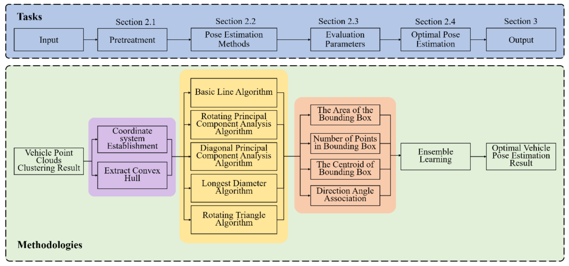
2. Methods
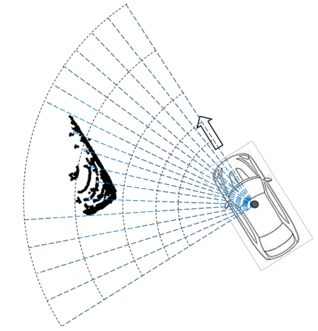
2.1. Pretreatment
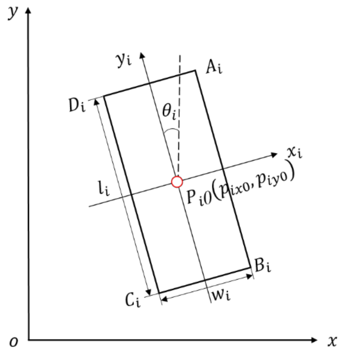
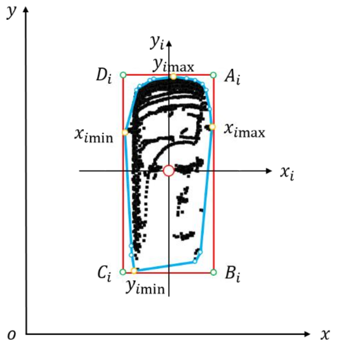
2.1.1. Establishment of Coordinate System
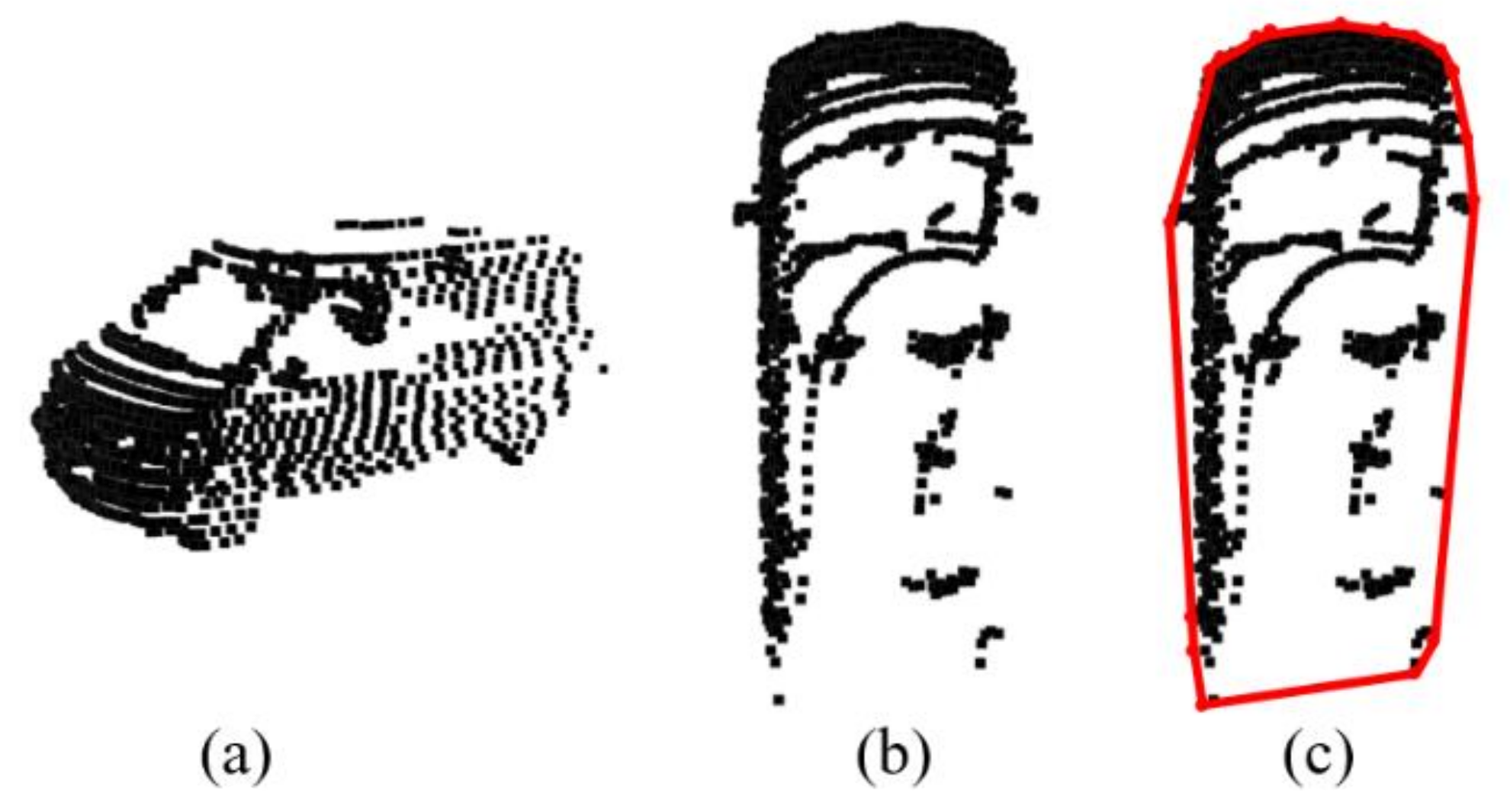
2.1.2. Extraction of Convex Hull
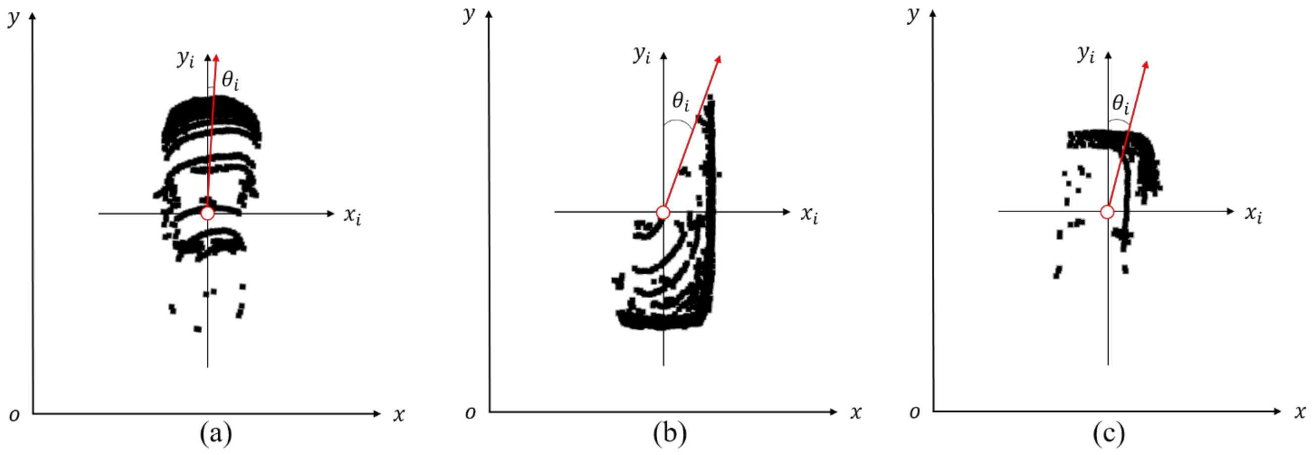
2.2. Vehicle Pose Estimation
2.2.1. Basic Line Algorithm
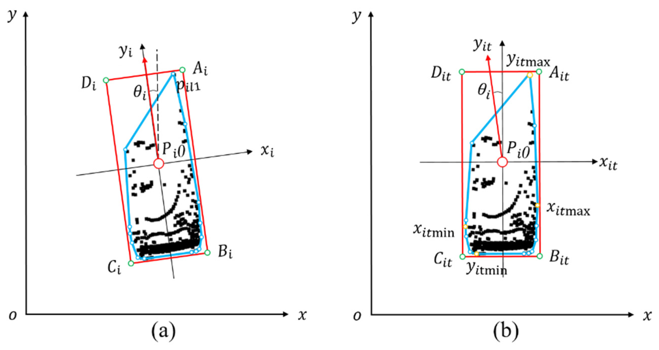
2.2.2. Pose Estimation Algorithms Based on PCA
- Basic principles and feasibility analysis of PCA
- Rotating Principal Component Analysis Algorithm
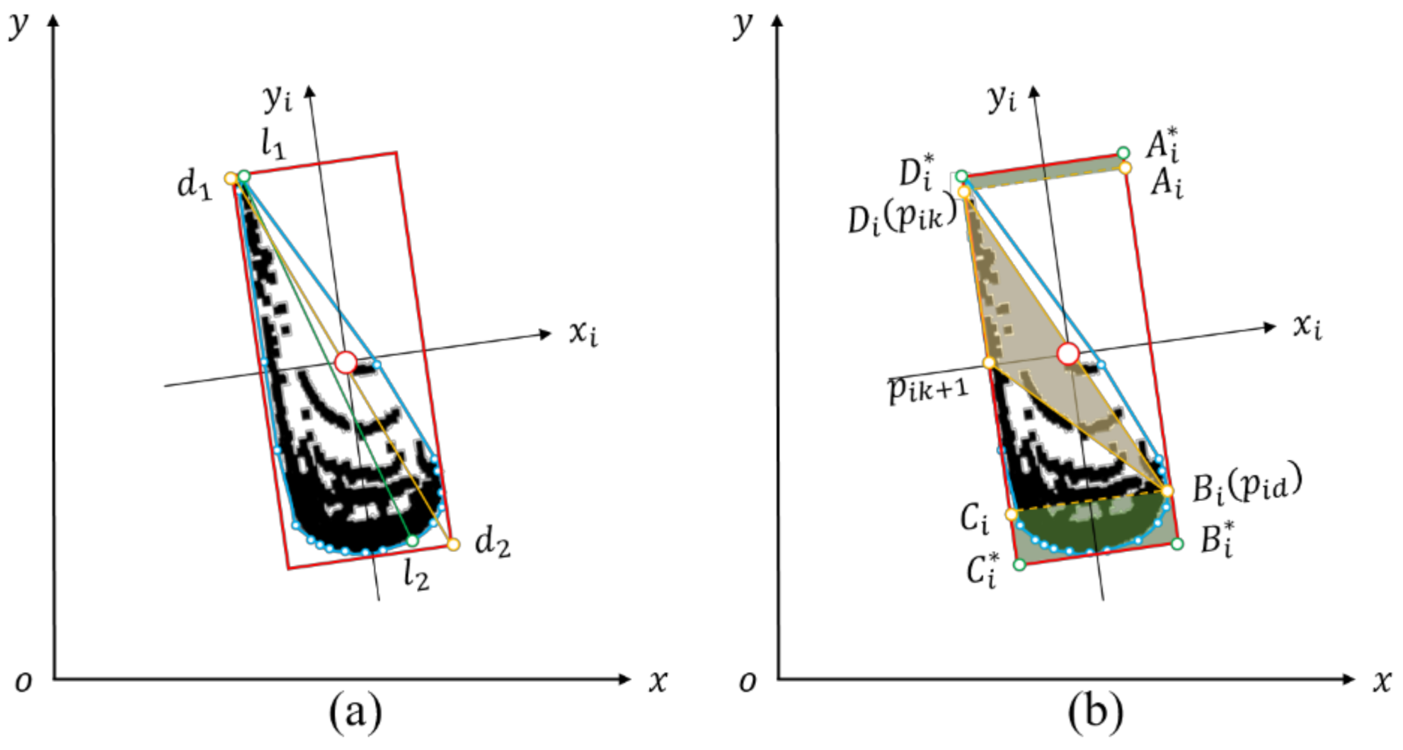
- Diagonal Principal Component Analysis Algorithm
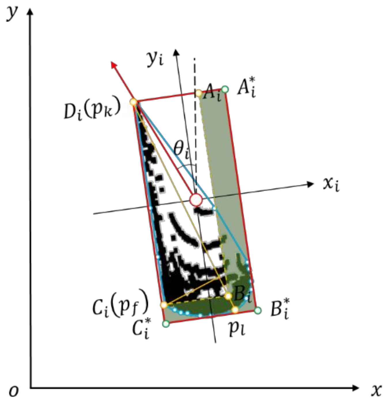
2.2.3. Longest Diameter Algorithm
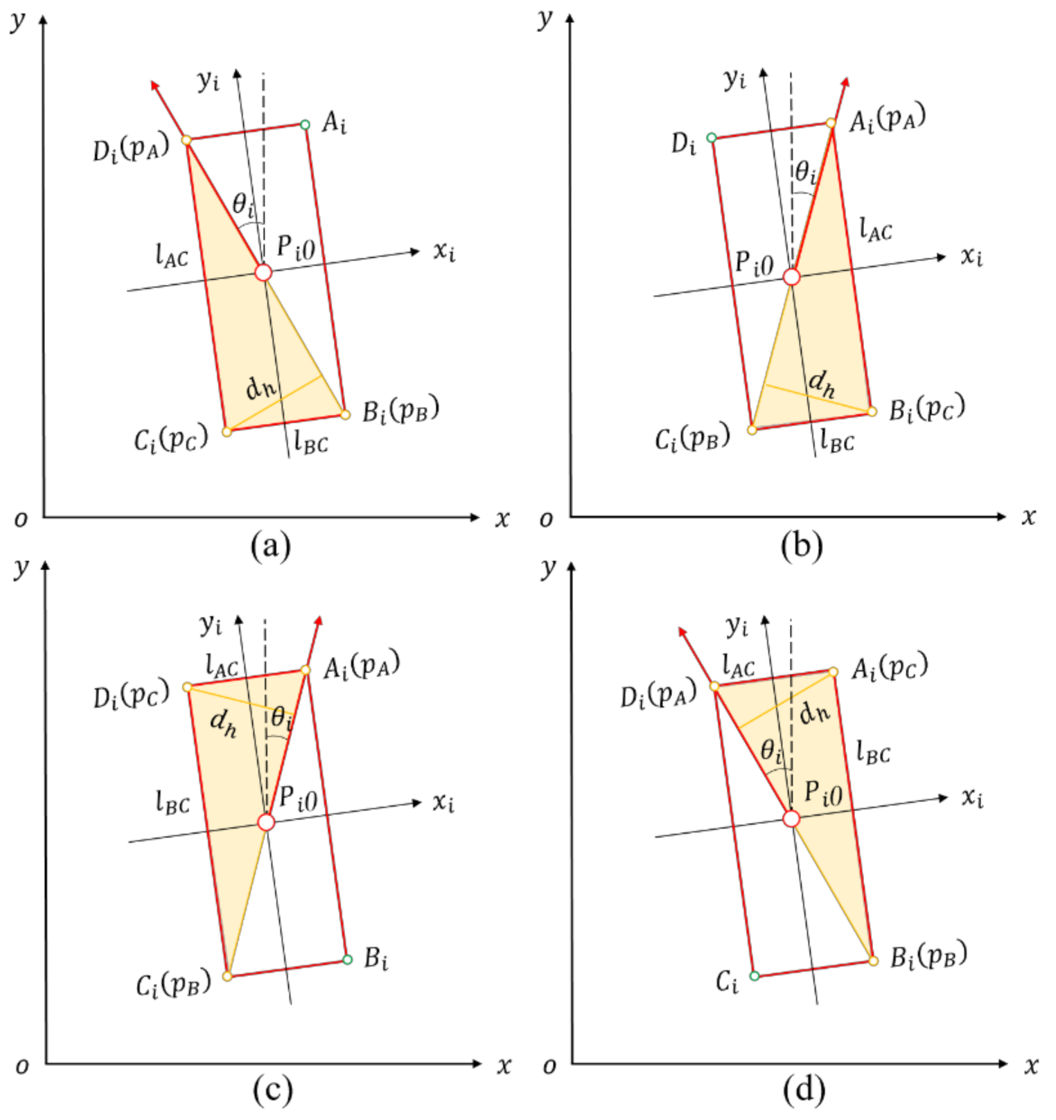
2.2.4. Rotating Triangle Algorithm
2.2.5. Comparison of Our Vehicle Pose Estimation Methods
2.3. Pose Estimation Evaluation Indexes
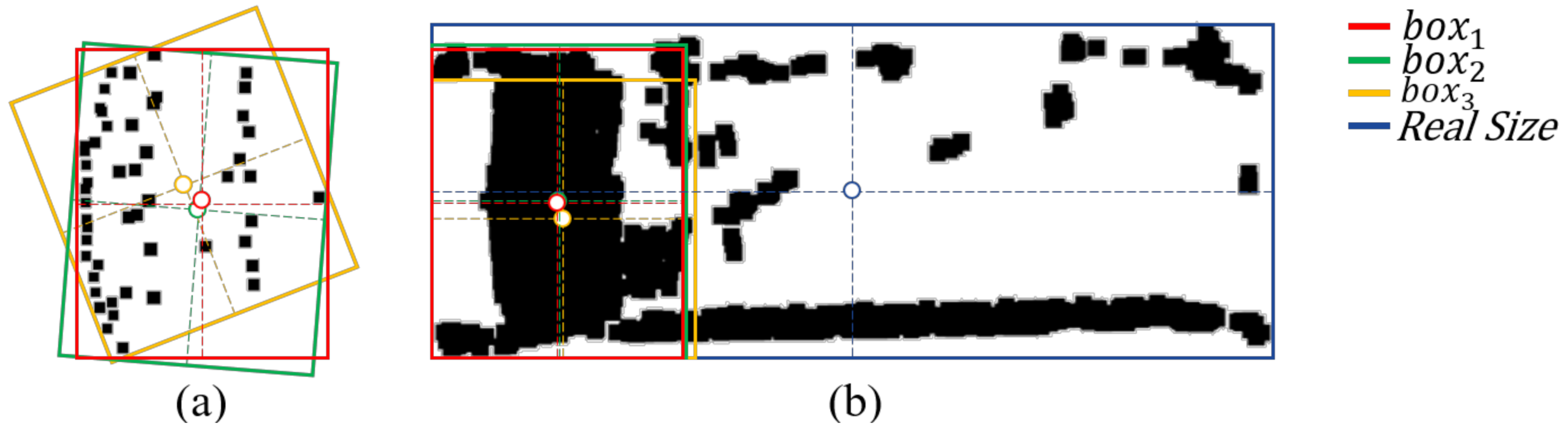
2.3.1. The Area of the Bounding Box
2.3.2. Number of Points in the Bounding Box
2.3.3. The Centroid of the Bounding Box
2.3.4. Direction Angle Association
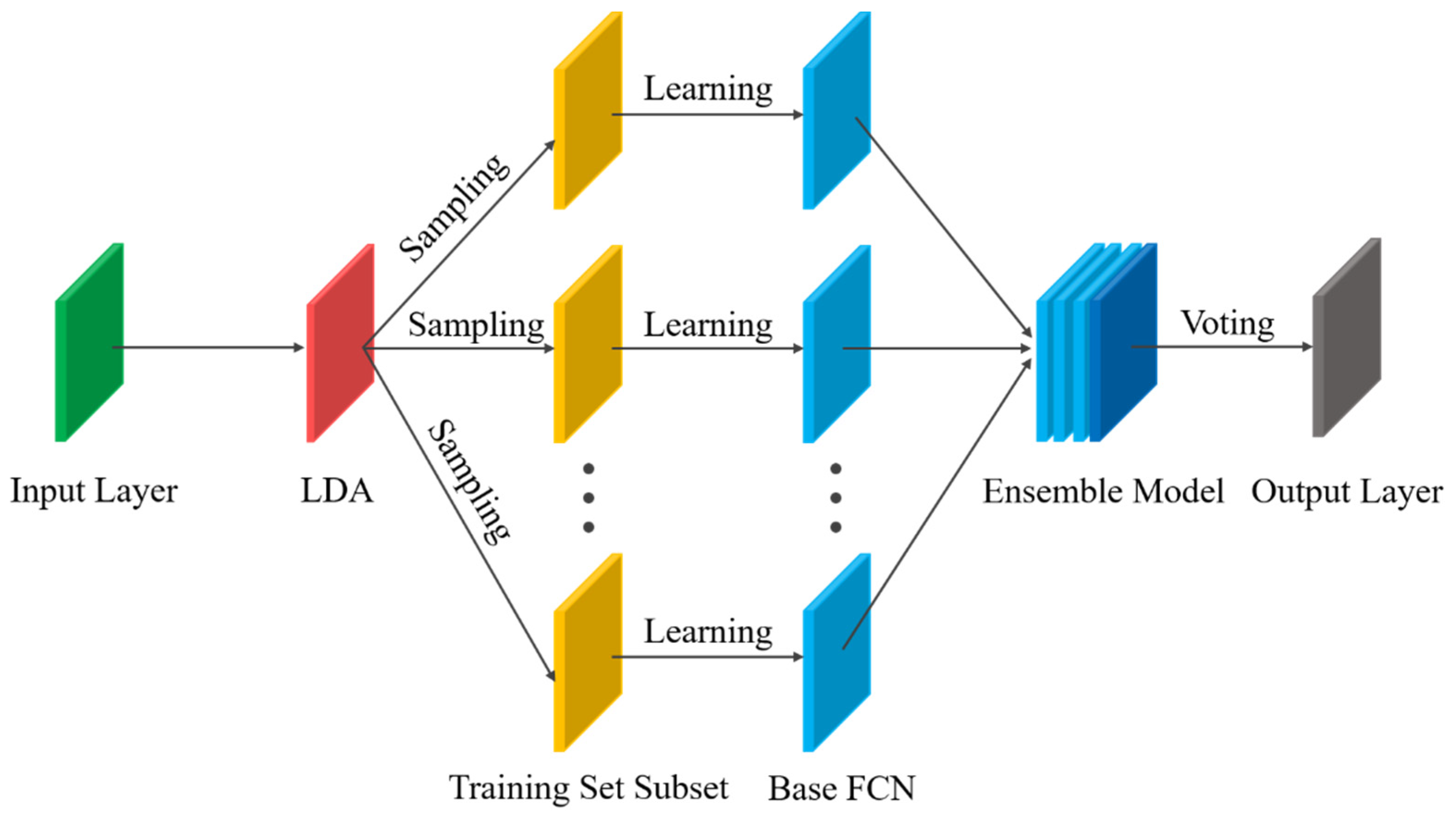
2.4. Optimal Vehicle Pose Estimation Method Based on Ensemble Learning
3. Experimental Results and Discussion
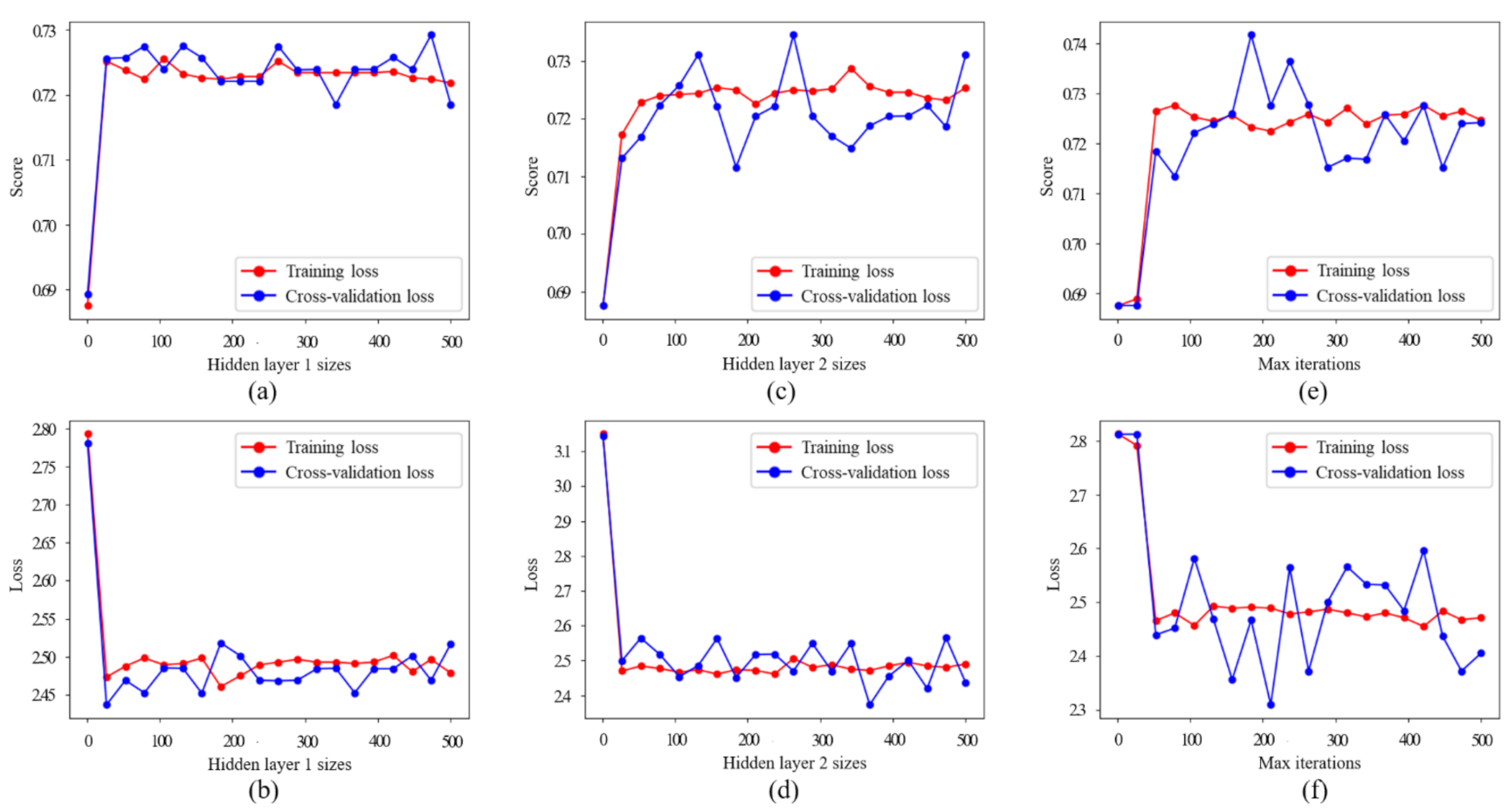
3.1. The Details of TS-OVPE Network
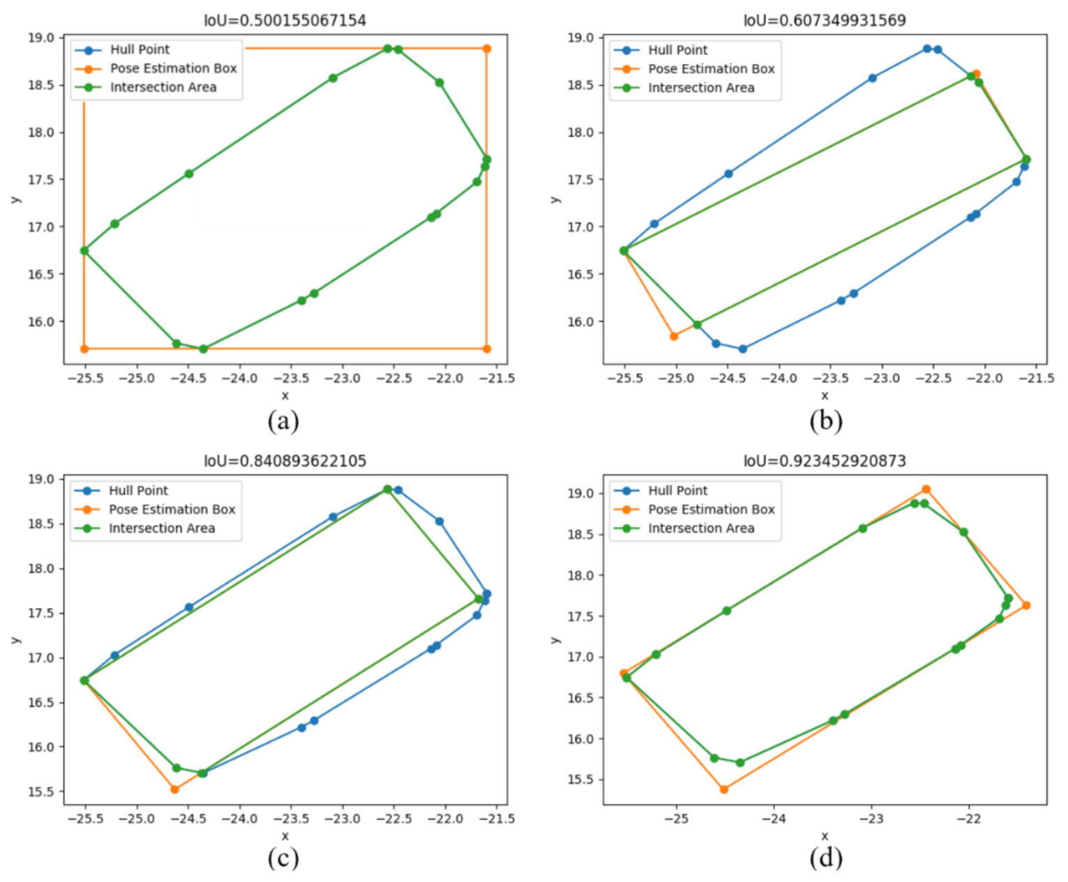
3.2. Evaluation Index of Pose Estimation Results: Polygon Intersection over Union
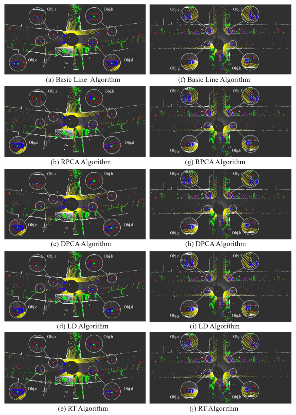
3.3. Experimental Results of SemanticKITTI Dataset
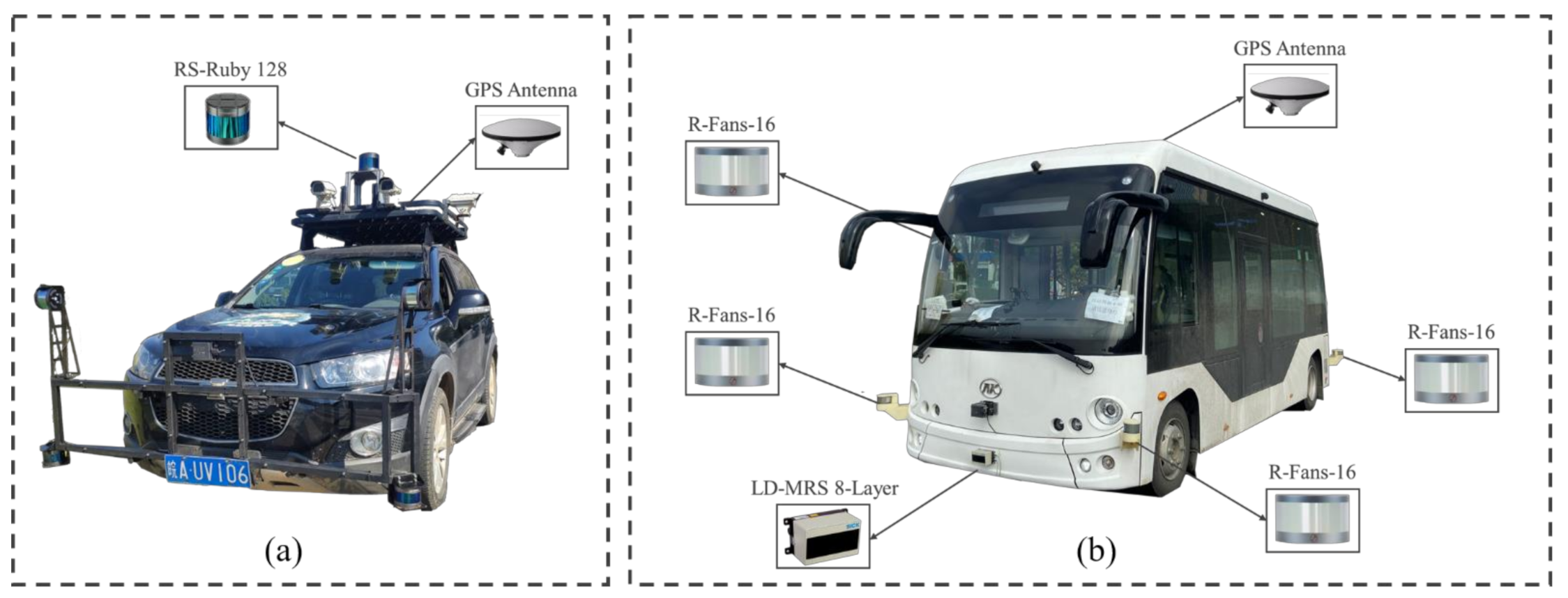
3.4. Experimental Results of Our Experimental Platform
4. Discussion
5. Conclusions
Author Contributions
Funding
Institutional Review Board Statement
Informed Consent Statement
Data Availability Statement
Conflicts of Interest
Abbreviations
| AV | Autonomous Vehicle |
| LiDAR | Light Detection and Ranging |
| TS-OVPE | Optimal Vehicle Pose Estimation Based on Time Series and Spatial Tightness |
| PCA | Principal Component Analysis |
| RPCA | Rotating Principal Component Analysis |
| DPCA | Diagonal Principal Component Analysis |
| LD | Longest Diameter |
| RT | Rotating Triangle |
| IoU | Intersection over Union |
| P-IoU | Polygon Intersection over Union |
| ROS | Robot Operating System |
| IMU | Inertial Measurement Unit |
References
- Khatab, E.; Onsy, A.; Varley, M.; Abouelfarag, A. Vulnerable objects detection for autonomous driving: A review. Integration 2021, 78, 36–48. [Google Scholar] [CrossRef]
- Su, Z.; Hui, Y.; Luan, T.H.; Liu, Q.; Xing, R. Deep Learning Based Autonomous Driving in Vehicular Networks. In The Next Generation Vehicular Networks, Modeling, Algorithm and Applications, 1st ed.; Springer: Cham, Switzerland, 2020; pp. 131–150. [Google Scholar] [CrossRef]
- Du, X.; Ang, M.H.; Karaman, S.; Rus, D. A general pipeline for 3d detection of vehicles. In Proceedings of the IEEE International Conference on Robotics and Automation (ICRA), Brisbane, Australia, 21–25 May 2018; pp. 3194–3200. [Google Scholar] [CrossRef] [Green Version]
- Du, L.; Ye, X.; Tan, X.; Feng, J.; Xu, Z.; Ding, E.; Wen, S. Associate-3Ddet: Perceptual-to-Conceptual Association for 3D Point Cloud Object Detection. In Proceedings of the IEEE/CVF Conference on Computer Vision and Pattern Recognition (CVPR), Seattle, WA, USA, 13–19 June 2020; pp. 13326–13335. [Google Scholar] [CrossRef]
- Tan, M.; Pang, R.; Le, Q.V. EfficientDet: Scalable and Efficient Object Detection. In Proceedings of the IEEE/CVF Conference on Computer Vision and Pattern Recognition (CVPR), Seattle, WA, USA, 13–19 June 2020; pp. 10778–10787. [Google Scholar] [CrossRef]
- Bochkovskiy, A.; Wang, C.-Y.; Liao, H.-Y.M. YOLOv4: Optimal Speed and Accuracy of Object Detection. arXiv 2020, arXiv:2004.10934. [Google Scholar]
- Wang, T.; Anwer, R.M.; Cholakkal, H.; Khan, F.S.; Pang, Y.; Shao, L. Learning rich features at high-speed for single-shot object detection. In Proceedings of the IEEE/CVF International Conference on Computer Vision (ICCV), Seoul, Korea, 27–28 October 2019; pp. 1971–1980. [Google Scholar] [CrossRef]
- Liu, S.; Huang, D. Receptive field block net for accurate and fast object detection. In Proceedings of the European Conference on Computer Vision (ECCV), Munich, Germany, 8–14 September 2018; pp. 385–400. [Google Scholar] [CrossRef] [Green Version]
- Ren, S.; He, K.; Girshick, R.; Sun, J. Faster R-CNN: Towards Real-Time Object Detection with Region Proposal Networks. IEEE Trans. Pattern Anal. Mach. Intell. 2017, 39, 1137–1149. [Google Scholar] [CrossRef] [Green Version]
- Shi, S.; Guo, C.; Jiang, L.; Wang, Z.; Shi, J.; Wang, X.; Li, H. PV-RCNN: Point-Voxel Feature Set Abstraction for 3D Object Detection. In Proceedings of the IEEE/CVF Conference on Computer Vision and Pattern Recognition (CVPR), Seattle, WA, USA, 13–19 June 2020; pp. 10526–10535. [Google Scholar] [CrossRef]
- Zhou, J.; Tan, X.; Shao, Z.; Ma, L. FVNet: 3D Front-View Proposal Generation for Real-Time Object Detection from Point Clouds. In Proceedings of the 12th International Congress on Image and Signal Processing, BioMedical Engineering and Informatics (CISP-BMEI), Kunshan, China, 19–21 October 2019; pp. 1–8. [Google Scholar] [CrossRef] [Green Version]
- Beltrán, J.; Guindel, C.; Moreno, F.M.; Cruzado, D.; García, F.; Escalera, A.D.L. BirdNet: A 3D Object Detection Framework from LiDAR Information. In Proceedings of the 21st International Conference on Intelligent Transportation Systems (ITSC), Maui, HI, USA, 4–7 November 2018; pp. 3517–3523. [Google Scholar] [CrossRef] [Green Version]
- Geiger, A.; Lenz, P.; Stiller, C.; Urtasun, R. Vision meets robotics: The KITTI dataset. Int. J. Robot. Res. 2013, 32, 1231–1237. [Google Scholar] [CrossRef] [Green Version]
- Wu, Y.; Wang, Y.; Zhang, S.; Ogai, H. Deep 3D Object Detection Networks Using LiDAR Data: A Review. IEEE Sensors J. 2021, 21, 1152–1171. [Google Scholar] [CrossRef]
- Huang, W.; Liang, H.; Lin, L.; Wang, Z.; Wang, S.; Yu, B.; Niu, R. A Fast Point Cloud Ground Segmentation Approach Based on Coarse-To-Fine Markov Random Field. IEEE Trans. Intell. Transp. Syst. 2021. Early Access. [Google Scholar] [CrossRef]
- Yang, H.; Wang, Z.; Lin, L.; Liang, H.; Huang, W.; Xu, F. Two-Layer-Graph Clustering for Real-Time 3D LiDAR Point Cloud Segmentation. Appl. Sci. 2020, 10, 8534. [Google Scholar] [CrossRef]
- Yang, J.; Zeng, G.; Wang, W.; Zuo, Y.; Yang, B.; Zhang, Y. Vehicle Pose Estimation Based on Edge Distance Using Lidar Point Clouds (Poster). In Proceedings of the 22th International Conference on Information Fusion (FUSION), Ottawa, ON, Canada, 2–5 July 2019; pp. 1–6. [Google Scholar]
- An, J.; Kim, E. Novel Vehicle Bounding Box Tracking Using a Low-End 3D Laser Scanner. IEEE Trans. Intell. Transp. Syst. 2021, 22, 3403–3419. [Google Scholar] [CrossRef]
- Li, Y.; Ibanez-Guzman, J. Lidar for Autonomous Driving: The Principles, Challenges, and Trends for Automotive Lidar and Perception Systems. IEEE Signal Process. Mag. 2020, 37, 50–61. [Google Scholar] [CrossRef]
- Li, Y.; Ma, L.; Zhong, Z.; Liu, F.; Chapman, M.A.; Cao, D.; Li, J. Deep Learning for LiDAR Point Clouds in Autonomous Driving: A Review. IEEE Trans. Neural Networks Learn. Syst. 2021, 32, 3412–3432. [Google Scholar] [CrossRef]
- Wen, C.; Sun, X.; Li, J.; Wang, C.; Guo, Y.; Habib, A. A deep learning framework for road marking extraction, classification and completion from mobile laser scanning point clouds. ISPRS J. Photogramm. Remote. Sens. 2019, 147, 178–192. [Google Scholar] [CrossRef]
- Kumar, B.; Pandey, G.; Lohani, B.; Misra, S.C. A multi-faceted CNN architecture for automatic classification of mobile LiDAR data and an algorithm to reproduce point cloud samples for enhanced training. ISPRS J. Photogramm. Remote. Sens. 2019, 147, 80–89. [Google Scholar] [CrossRef]
- Xu, F.; Liang, H.; Wang, Z.; Lin, L.; Chu, Z. A Real-Time Vehicle Detection Algorithm Based on Sparse Point Clouds and Dempster-Shafer Fusion Theory. In Proceedings of the IEEE International Conference on Information and Automation (ICIA), Wuyi Mountain, China, 11–13 August 2018; pp. 597–602. [Google Scholar] [CrossRef]
- Wittmann, D.; Chucholowski, F.; Lienkamp, M. Improving lidar data evaluation for object detection and tracking using a priori knowledge and sensorfusion. In Proceedings of the 11th International Conference on Informatics in Control, Automation and Robotics (ICINCO), Vienna, Austria, 1–3 September 2014; pp. 794–801. [Google Scholar] [CrossRef]
- Zhao, C.; Fu, C.; Dolan, J.M.; Wang, J. L-Shape Fitting-based Vehicle Pose Estimation and Tracking Using 3D-LiDAR. IEEE Trans. Intell. Veh. 2021. Early Access. [Google Scholar] [CrossRef]
- MacLachlan, R.; Mertz, C. Tracking of Moving Objects from a Moving Vehicle Using a Scanning Laser Rangefinder. In Proceedings of the 2006 IEEE Intelligent Transportation Systems Conference (ITSC), Toronto, ON, Canada, 17–20 September 2006; pp. 301–306. [Google Scholar] [CrossRef] [Green Version]
- Shen, X.; Pendleton, S.; Ang, M.H. Efficient L-shape fitting of laser scanner data for vehicle pose estimation. In Proceedings of the 2015 IEEE 7th International Conference on Cybernetics and Intelligent Systems (CIS) and IEEE Conference on Robotics, Automation and Mechatronics (RAM), Angkor Wat, Cambodia, 15–17 July 2015; pp. 173–178. [Google Scholar] [CrossRef]
- Wang, Z.; Wu, Y.; Niu, Q. Multi-Sensor Fusion in Automated Driving: A Survey. IEEE Access 2019, 8, 2847–2868. [Google Scholar] [CrossRef]
- Wu, T.; Hu, J.; Ye, L.; Ding, K. A Pedestrian Detection Algorithm Based on Score Fusion for Multi-LiDAR Systems. Sensors 2021, 21, 1159. [Google Scholar] [CrossRef]
- Zhang, X.; Xu, W.; Dong, C.; Dolan, J.M. Efficient L-shape fitting for vehicle detection using laser scanners. In Proceedings of the 2017 IEEE Intelligent Vehicles Symposium (IV), Redondo Beach, CA, USA, 11–14 June 2017; pp. 54–59. [Google Scholar] [CrossRef]
- Qu, S.; Chen, G.; Ye, C.; Lu, F.; Wang, F.; Xu, Z.; Gel, Y. An Efficient L-Shape Fitting Method for Vehicle Pose Detection with 2D LiDAR. In Proceedings of the IEEE International Conference on Robotics and Biomimetics (ROBIO), Kuala Lumpur, Malaysia, 12–15 December 2018; pp. 1159–1164. [Google Scholar] [CrossRef] [Green Version]
- Kim, D.; Jo, K.; Lee, M.; Sunwoo, M. L-Shape Model Switching-Based Precise Motion Tracking of Moving Vehicles Using Laser Scanners. IEEE Trans. Intell. Transp. Syst. 2017, 19, 598–612. [Google Scholar] [CrossRef]
- Chen, T.; Wang, R.; Dai, B.; Liu, D.; Song, J. Likelihood-Field-Model-Based Dynamic Vehicle Detection and Tracking for Self-Driving. IEEE Trans. Intell. Transp. Syst. 2016, 17, 3142–3158. [Google Scholar] [CrossRef]
- Chen, T.; Dai, B.; Liu, D.; Fu, H.; Song, J.; Wei, C. Likelihood-Field-Model-Based Vehicle Pose Estimation with Velodyne. In Proceedings of the 2015 IEEE 18th International Conference on Intelligent Transportation Systems (ITSC), Gran Canaria, Spain, 15–18 September 2015; pp. 296–302. [Google Scholar] [CrossRef]
- Naujoks, B.; Wuensche, H. An Orientation Corrected Bounding Box Fit Based on the Convex Hull under Real Time Constraints. In Proceedings of the 2018 IEEE Intelligent Vehicles Symposium (IV), Changshu, China, 26–30 June 2018; pp. 1–6. [Google Scholar] [CrossRef]
- Liu, K.; Wang, W.; Tharmarasa, R.; Wang, J. Dynamic Vehicle Detection with Sparse Point Clouds Based on PE-CPD. IEEE Trans. Intell. Transp. Syst. 2019, 20, 1964–1977. [Google Scholar] [CrossRef]
- Sklansky, J. Finding the convex hull of a simple polygon. Pattern Recognit. Lett. 1982, 1, 79–83. [Google Scholar] [CrossRef]
- Zhao, H.; Zhang, Q.; Chiba, M.; Shibasaki, R.; Cui, J.; Zha, H. Moving object classification using horizontal laser scan data. In Proceedings of the IEEE International Conference on Robotics and Automation (ICRA), Kobe, Japan, 12–17 May 2009; pp. 2424–2430. [Google Scholar] [CrossRef]
- Behley, J.; Garbade, M.; Milioto, A.; Quenzel, J.; Behnke, S.; Stachniss, C.; Gall, J. Semantickitti: A dataset for semantic scene understanding of lidar sequences. In Proceedings of the IEEE/CVF International Conference on Computer Vision (ICCV), Seoul, Korea, 27–28 October 2019; pp. 9297–9307. [Google Scholar] [CrossRef] [Green Version]
- Geiger, A.; Lenz, P.; Urtasun, R. Are we ready for autonomous driving? The KITTI vision benchmark suite. In Proceedings of the 2012 IEEE Conference on Computer Vision and Pattern Recognition (CVPR), Providence, RI, USA, 16–21 June 2012; pp. 3354–3361. [Google Scholar] [CrossRef]
- Arya, A. 3D-LIDAR Multi Object Tracking for Autonomous Driving: Multi-target Detection and Tracking under Urban Road Uncertainties. Master’s Thesis, Delft University of Technology, Delft, The Netherlands, 2017. [Google Scholar]
- Lee, H.; Chae, H.; Yi, K. A Geometric Model based 2D LiDAR/Radar Sensor Fusion for Tracking Surrounding Vehicles. IFAC-PapersOnLine 2019, 52, 130–135. [Google Scholar] [CrossRef]
- Glowinski, S.; Krzyzynski, T.; Bryndal, A.; Maciejewski, I. A Kinematic Model of a Humanoid Lower Limb Exoskeleton with Hydraulic Actuators. Sensors 2020, 20, 6116. [Google Scholar] [CrossRef] [PubMed]
- Slowak, P.; Kaniewski, P. Stratified Particle Filter Monocular SLAM. Remote. Sens. 2021, 13, 3233. [Google Scholar] [CrossRef]


| Algorithm | Small Curved Roads | Crossroads | ||||||
|---|---|---|---|---|---|---|---|---|
| Obj.a | Obj.b | Obj.c | Obj.d | Obj.e | Obj.f | Obj.g | Obj.h | |
| Basic Line | √ | √ | × | √ | × | × | × | × |
| RPCA | √ | × | × | √ | √ | × | √ | √ |
| DPCA | × | √ | × | × | × | √ | × | × |
| LD | × | √ | √ | × | √ | × | √ | √ |
| RT | √ | × | √ | √ | √ | × | √ | √ |
| Precision | Recall | F1 Score | |
|---|---|---|---|
| Initial Base Learner | 42.79% | 65.42% | 51.74% |
| Optimized Base Learner | 65.09% | 67.50% | 66.27% |
| Ensemble Learning | 71.95% | 72.50% | 72.22% |
| Straight Road | Curved Road | All Road | |
|---|---|---|---|
| Number of static vehicles | 53,423 | 13,389 | 66,812 |
| Number of dynamic vehicles | 201 | 72 | 273 |
| Total number of vehicles | 53,624 | 13,461 | 67,085 |
| Straight Road | Curved Road | All Road | |
|---|---|---|---|
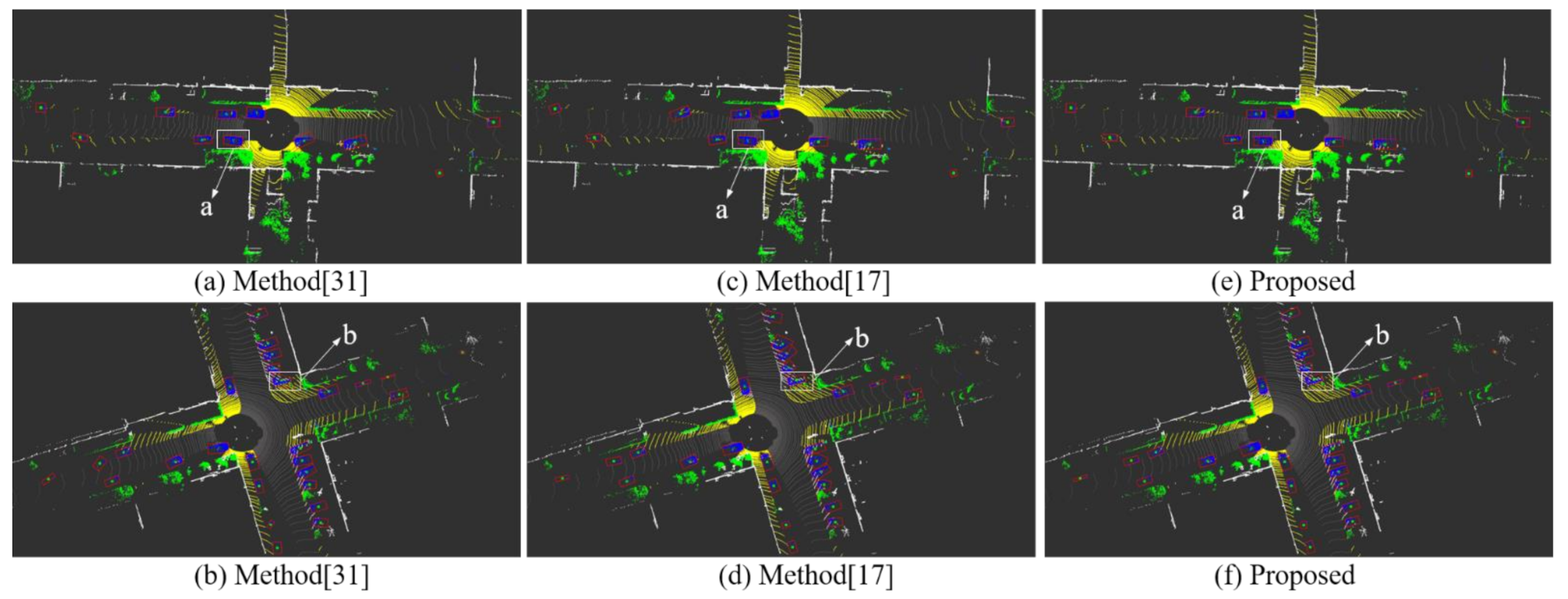
| Method [31] | 67.24% | 66.54% | 67.12% |
| Method [17] | 63.11% | 61.05% | 62.70% |
| Proposed | 72.32% | 72.57% | 72.37% |
| Parameters | "Smart Pioneer" SUV Platform | "Smart Pioneer" Minibus Platform | |
|---|---|---|---|
| Basic Information | Vehicle Brand | Chevrolet | ANKAI |
| Power Type | Petrol Car | Blade Electric Vehicles | |
| Length (mm) | 4673 | 6605 | |
| Width (mm) | 1868 | 2320 | |
| Height (mm) | 1756 | 2870 | |
| Wheel Base (mm) | 2705 | 4400 | |
| Curb Weight (kg) | 1822 | 5500 | |
| Main Performance | Max. Speed (km/h) | 60 | 30 |
| Position Control Error (mm) | ±300 (60km/h) | ±300 (30km/h) | |
| Speed Control Error (km/h) | ±0.5 | ±0.5 | |
| Development Information | Operating System | Linux (Ubuntu 16.04) Robot Operating System (ROS) | |
| Hardware | Intel I7-8700 CPU and 16 GB RAM | ||
| Road Types | Methods | Pose Estimation Results | Object Tracking Results | ||||||||
|---|---|---|---|---|---|---|---|---|---|---|---|
| Shape Error (m) | Position Error (m) | Heading Error (Deg) | Speed Error (m/s) | Speed Direction Error (Deg) | |||||||
| Mean | Std | Mean | Std | Mean | Std | Mean | Std | Mean | Std | ||
| All road | Method [31] | 1.55 | 0.81 | 1.46 | 0.38 | 40.25 | 54.09 | 0.27 | 0.40 | 1.56 | 2.91 |
| Method [17] | 1.57 | 0.98 | 1.45 | 0.39 | 50.78 | 58.05 | 0.36 | 0.54 | 2.83 | 4.99 | |
| Proposed | 1.54 | 0.82 | 1.44 | 0.39 | 28.38 | 42.41 | 0.26 | 0.39 | 1.50 | 2.59 | |
| Curved road | Method [31] | 0.87 | 0.68 | 1.14 | 0.38 | 34.93 | 52.12 | 0.37 | 0.54 | 2.98 | 4.08 |
| Method [17] | 0.88 | 0.92 | 1.15 | 0.39 | 47.14 | 56.45 | 0.56 | 0.79 | 4.30 | 6.65 | |
| Proposed | 0.85 | 0.66 | 1.13 | 0.39 | 13.29 | 22.92 | 0.36 | 0.53 | 2.62 | 3.44 | |
| Straight road | Method [31] | 2.35 | 0.50 | 1.77 | 0.16 | 52.57 | 60.79 | 0.22 | 0.33 | 0.39 | 0.49 |
| Method [17] | 2.38 | 0.64 | 1.77 | 0.16 | 59.26 | 62.11 | 0.27 | 0.39 | 0.84 | 1.26 | |
| Proposed | 2.32 | 0.48 | 1.77 | 0.16 | 38.15 | 51.92 | 0.21 | 0.32 | 0.38 | 0.55 | |
Publisher’s Note: MDPI stays neutral with regard to jurisdictional claims in published maps and institutional affiliations. |
© 2021 by the authors. Licensee MDPI, Basel, Switzerland. This article is an open access article distributed under the terms and conditions of the Creative Commons Attribution (CC BY) license (https://creativecommons.org/licenses/by/4.0/).
Share and Cite
Wang, H.; Wang, Z.; Lin, L.; Xu, F.; Yu, J.; Liang, H. Optimal Vehicle Pose Estimation Network Based on Time Series and Spatial Tightness with 3D LiDARs. Remote Sens. 2021, 13, 4123. https://doi.org/10.3390/rs13204123
Wang H, Wang Z, Lin L, Xu F, Yu J, Liang H. Optimal Vehicle Pose Estimation Network Based on Time Series and Spatial Tightness with 3D LiDARs. Remote Sensing. 2021; 13(20):4123. https://doi.org/10.3390/rs13204123
Chicago/Turabian StyleWang, Hanqi, Zhiling Wang, Linglong Lin, Fengyu Xu, Jie Yu, and Huawei Liang. 2021. "Optimal Vehicle Pose Estimation Network Based on Time Series and Spatial Tightness with 3D LiDARs" Remote Sensing 13, no. 20: 4123. https://doi.org/10.3390/rs13204123
APA StyleWang, H., Wang, Z., Lin, L., Xu, F., Yu, J., & Liang, H. (2021). Optimal Vehicle Pose Estimation Network Based on Time Series and Spatial Tightness with 3D LiDARs. Remote Sensing, 13(20), 4123. https://doi.org/10.3390/rs13204123