Abstract
The Mars Science Laboratory rover Curiosity landed in Gale crater (Mars) in August 2012. It has since been studying the lower part of the 5 km-high sedimentary pile that composes Gale’s central mound, Aeolis Mons. To assess the sedimentary record, the MSL team mainly uses a suite of imagers onboard the rover, providing various pixel sizes and fields of view from close to long-range observations. For this latter, we notably use the Remote Micro Imager (RMI), a subsystem of the ChemCam instrument that acts as 700 mm-focal length telescope, providing the smallest angular pixel size of the set of cameras on the Remote Sensing Mast. The RMI allows observations of remote outcrops up to a few kilometers away from the rover. As retrieving 3D information is critical to characterize the structures of the sedimentary deposits, we describe in this work an experiment aiming at computing for the first time with RMI Digital Outcrop Models of these distant outcrops. We show that Structure-from-Motion photogrammetry can successfully be applied to suitable sets of individual RMI frames to reconstruct the 3D shape and relief of these distant outcrops. These results show that a dedicated set of observations can be envisaged to characterize the most interesting geological features surrounding the rover.
1. Introduction
Gale crater on Mars records a large section of sedimentary rocks, mainly represented by the 5-km-thick sequence of Mount Sharp (Aeolis Mons). It is home to the Mars Science Laboratory (MSL) rover Curiosity, whose mission is to help characterize the geological record using its suite of instruments, seeking out past presence of habitable conditions at a time when liquid water was abundant at the surface of the red planet [1,2]. Its mission therefore critically relies on the capacity of the team in deciphering the multi-scale geomorphological and sedimentological features present there to characterize the past environments.
To that end, we are taking advantage of all the various imaging instruments at our disposal aboard the rover, from the navigation cameras (Navcam) [3], to the color science imagers Mastcam [4,5] and to the Remote Micro Imager (RMI) subsystem of the ChemCam instrument [6,7]. This suite of instruments with nested fields of view allows us to obtain multi-scale close-range to remote observations. This multi-scale imaging capacity is particularly important to characterize the natural rock exposures on Mars. Due to traversability issues and resources/time optimization constraints, the rover cannot access specific zones despite their scientific interest. Their exploration therefore solely relies on orbital data complemented by remote imaging by the rover from several hundreds of meters up to several kilometers, using onboard cameras (Mastcam, RMI [8]).
This is notably the case of the lower sulfates unit of lower Mount Sharp, an area of great interest due to the previous orbital detection of sulfate-bearing strata [9,10]. Orbital data combined with rover-based observations revealed that the sulfate-bearing unit coincides with a major change of depositional environments followed by alternation of wet and dry conditions rather than a monotonous aridification during the Hesperian epoch [11]. However, this distant area has not yet been reached by the rover, so current observations were notably supported using long-distance imaging capabilities of the RMI sub-system of the ChemCam instrument. With a focal length of 700 mm, the RMI telescope complements the color Mastcam imagers with higher spatial resolution views of rocks cropping out several hundred meters up to a few kilometers away from the rover. This long-range imaging capacity is also useful in planning guidance of the rover. While these long-distance observations pointed at the sulfate-bearing unit revealed the presence of sub-metric-scale cross-stratifications, deflation surfaces, and diagenetic features, the resulting images lack depth due to the distance. Yet such 3D information can be critical in characterizing and understanding the sedimentary processes which generated these structures. 3D views enable a more quantitative interpretation of the sedimentary structures (e.g., scale, transport directions, etc.). We thus highlight here the need for a way to better investigate the various readable but distant outcrops using existing imagery produced in situ by Curiosity.
In this work, we propose for the first-time to create Digital Outcrop Models (DOM) of remote outcrops using the long-distance imagery from RMI’s telescope. We use Structure-from-Motion photogrammetry, a method usually performed on close-range geologic features observed with other imagers onboard the rover (MAHLI, Mastcam, Navcam [12]). To conduct this experiment, we apply photogrammetric treatment to specific sets of repeated long-distance RMI observations that we specifically targeted on the sulfate-bearing units. We therefore demonstrate the feasibility of this concept. The use of this technique to produce 3D models of remote geological exposures might have critical implication in helping to assess and to characterize the paleoenvironmental record studied with the Curiosity rover.
2. Localization and Area of Interest
Gale crater is a ~155 km-wide impact crater (Figure 1a) situated near the crustal dichotomy boundary of Mars, separating southern cratered terrain and northern smoother lowlands. The Curiosity rover of the MSL mission landed in August 2012 in the northern part of this crater (Figure 1a) in the Aeolis Palus region. Since then, the rover explored the geological record of Aeolis Palus and the lower flanks of the Mount Sharp (Aeolis Mons) along a ~25 km-long traverse. This sedimentary sequence revealed the existence of past lacustrine to fluvial depositional systems [1,2,13,14,15,16,17], but also some levels deposited in dryer aeolian settings [18]. The rover is currently starting the exploration of the lower sulfates unit of Mount Sharp (Figure 1b,c), a part of the sedimentary pile that has only been characterized by orbital data [9,10] or by remote long-distance imaging using the onboard cameras of the rover [8,11]. These observations show the presence of large-scale sedimentary structures, possibly associated with ancient aeolian depositional settings [11], but also the presence of younger yardang structures linked to wind abrasion [19]. Here, we focus on long-distance observations performed using RMI on the lower sulfate unit buttes above the Glen Torridon region where the rover was situated at the time the images were taken (cf. Figure 1b,c).
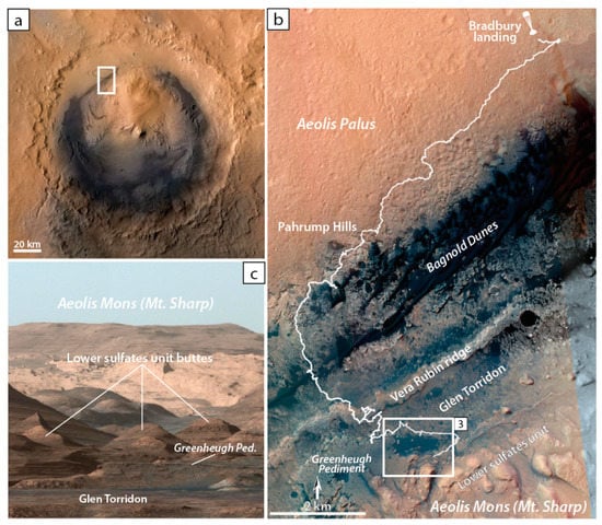
Figure 1.
Localization of the studied area on Mars. (a) Orbital image of the Gale crater. The white box represents the area of operations of the Curiosity rover. (b) View of path followed by the rover (white line) since Bradbury landing in August 2012 and up to the lower sulfate unit transition (as of July 2021). (c) Panoramic view from Aeolis Palus (Photo-journal image PIA19912, https://photojournal.jpl.nasa.gov/catalog/PIA19912, accessed on 8 August 2021) showing the vertical succession of the major units in Mount Sharp stratigraphy, notably highlighting the location of Glen Torridon region and the lower sulfates unit.
3. Data and Methods
3.1. Instruments and Products
The Curiosity rover is equipped with 17 cameras serving multiple purpose from determining trafficability along its traverse to multi-scale scientific observations for scientific remote sensing investigations; we mainly use the five cameras situated on the 2-m high Remote Sensing Mast (RSM) of the rover: the Navcam pair, the Mastcam pair, and ChemCam’s RMI (Figure 2a). The Navcam pair provide wide-angle stereo greyscale imagery (Table 1; Figure 2b) that can be used to produce close to mid-range 3D models of the rover’s surroundings [3,12,20]. The Mastcam pair provide high-resolution color imagery (Table 1; Figure 2b) to allow detailed scientific observations [4,5]. These cameras can be operated to obtain stereo mosaics [21] or even 3D DOM [12] but, contrary to the Navcam pair, their different focal length leads to a restricted field of acquisition of the 3D information. Finally, the RMI is a sub-system of the ChemCam instrument. Its main role is to image the targets analyzed by the Laser-Induced Breakdown Spectrometry [6,22], allowing close inspection of the analyzed rock (Figure 2b), its texture, and the markings left by the laser shots. Whereas RMI was not originally designed to observe at long distance, its 700 mm focal length appeared to be useful when pointing the telescope at remote objects (Table 1; [7]). In that role, the RMI can produce highly detailed greyscale views of outcrops up to several kilometers away (a ~60 km-record observation having recently been achieved [23]). As the pixel size of the RMI is 3.7× smaller than that of the M-100 [7], this instrument provides a complementary imaging capacity of the distant geological features with a very high resolution, but with a reduced field of view. The white box in the color Mastcam mosaic of Figure 2c (upper panel) highlights the area imaged by a composite RMI mosaic made from two merged observations (15 × 3 and 10 × 3 mosaics, lower panel in Figure 2c). With RMI, it is possible to see more details, such as meter-scale cross-stratifications and individual blocks highlighted in the detail boxes at the bottom of Figure 2c, that were not visible on the Mastcam image. This capacity is critical to characterize structures from long-distances and/or of outcrops inaccessible for the rover. However, unlike the Navcam and Mastcam pairs, the RMI is not natively capable of generating stereo-images to provide a 3D view of the imaged outcrops.
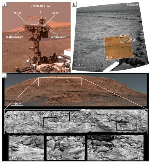
Figure 2.
(a) Detail of a “selfie” picture of Curiosity taken on sol 1943 by the MAHLI camera, showing the Remote Sensing Mast of the rover and the position of its main imaging instruments: Navcam, Mastcam and RMI (base image PIA22207, https://photojournal.jpl.nasa.gov/catalog/pia22207, accessed on 5 October 2021). (b) Composite image showing the variations in resolution, color, and field of view of the different Navcam, Mastcam and RMI imagers (images CR0_412749646PRC_F0060000CCAM02171L1, 0198MR0010070380202807E01, 0170ML0009050660104745E01, NLA_412415874EDR_F0060000NCAM12754M1). (c) Upper part: Mastcam (M-34) color mosaic of a large butte in the lower sulfates unit (Mastcam image sol03154_ML_100270); Lower part: composite RMI mosaic (images ccam3151 and ccam4153) corresponding to the white box in the Mastcam mosaic. RMI shows a higher level of details, allowing to distinguish down to meter-scale cross-stratifications and individual blocks (bottom detail boxes) from several hundred meters.

Table 1.
Main optical parameters of the Navcam, Mastcam and RMI imagers onboard Curiosity.
3.2. Digital Outcrop Modelling
When studying a geological outcrop, 3D information can be critical to characterize and understand the conditions that lead to the formation and/or alteration of the outcrop. This is particularly true in the case of the detrital depositional record encountered in Gale crater and the identification of sedimentary induced structures. However, this 3D information is not readily accessible when studying Martian outcrops from orbit and/or from rover-derived data. To compensate for the impossibility to observe these features “in person”, one solution is to digitally recreate the 3D shape of the explored outcrops from the data gathered by the rover.
To compute these DOMs, we use Structure-from-Motion (SfM) photogrammetry. This technique relies on a suite of algorithms able to recreate an accurate 3D representation of an object from a set of overlapping 2D images [24]. SfM photogrammetry is particularly well suited for geological purposes and is commonly used both on Earth [25,26,27,28,29], and in the planetary community [30,31]. In the case of the Gale crater, several successful examples of DOM reconstruction to characterize the sedimentary record have already been performed using Navcam [20], MAHLI [32], Mastcam [18] or a combination of these instruments [12,33].
In this work, we apply this method to images taken by the RMI telescope, in order to reconstruct the 3D shape of remote and inaccessible outcrops situated several hundred meters away from the rover. For the SfM process, we are using the commercial Agisoft Metashape Professional software v.1.7.1 (Agisoft LLC, St. Petersburg, Russia) [34].
3.3. Targets on the Lower Sulfates Unit
For this imaging experiment, we focus on two remote outcrops belonging to the lower sulfates unit, higher up the section of Mount Sharp (cf. Figure 2c and Figure 3a)). Each outcrop was imaged twice with RMI mosaics, taken from different viewpoints while the rover was situated in the Glen Torridon region (cf. Figure 2b and Figure 3a). To cope with the important distance, and with the necessity to obtain two widely different points of view for the overlapping images, we use a several hundred meters “virtual baseline”, represented by successive position of the rover along its traverse (Figure 3a). This baseline introduces parallax effects which allow the subsequent retrieval of 3D information.
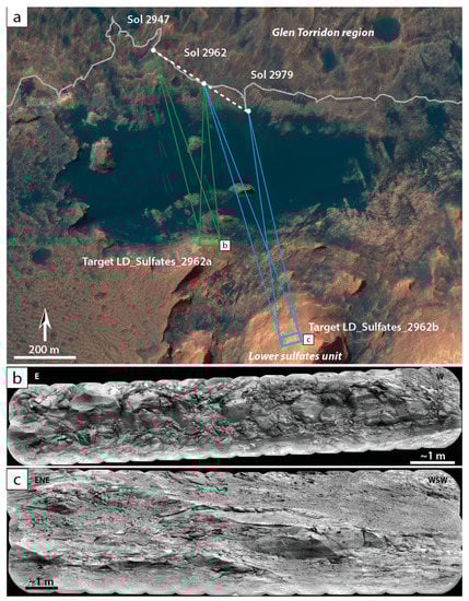
Figure 3.
(a) Detailed view of the eastern Glen Torridon region from where the RMI mosaics have been taken. The grey line represents the rover traverse; Green: successive positions of the rover to acquire the target LD_Sulfates_2692a, illustrated in (b); Blue: successive position of the rover to acquire the target LD_Sulfates_2962b, illustrated in (c); Dashed white line represents the “virtual baselines” set between two successive positions of the rover.
The first outcrop (LD_Sulfates_2962a on Figure 3a, illustrated in Figure 3b) was imaged on Sol (mission Martian day) 2947 and on Sol 2962 by mosaics labeled LD_Sulfates_2947b and LD_Sulfates_2962a, respectively (Table 1). The outcrop is situated between ~510 and ~650 m away from the rover, with a virtual baseline of ~200 m (Table 1, Figure 3a).
The second outcrop (LD_Sulfates_2962b on Figure 3a, illustrated in Figure 3c) was imaged on Sol 2962 and on Sol 2979 by mosaics labeled LD_Sulfates_2962b and LD_Sulfates_2979a, respectively (Table 1). This second outcrop is situated between ~760 and ~875 m away from the rover, with a virtual baseline of ~175 m (Table 1, Figure 3a).
4. Processing Chain
4.1. Imagery Dataset
Individual images taken by ChemCam’s RMI can be downloaded either from the JPL’s MSL RAW images library (https://mars.nasa.gov/msl/multimedia/raw-images/, accessed on 5 October 2021) or from the Planetary Data System (PDS; https://pds-geosciences.wustl.edu/missions/msl/, accessed on 5 October 2021). Images from the PDS are provided in the IMG exchange format, and therefore need to be converted beforehand using the small IMG2PNG command-line software utility (available at: http://bjj.mmedia.is/utils/img2png/, accessed on 5 October 2021). Preprocessed mosaics are also provided on the PDS in PNG format at https://pds-geosciences.wustl.edu/msl/msl-m-chemcam-libs-4_5-rdr-v1/mslccm_1xxx/extras/rmi_mosaics/, accessed on 5 October 2021. The RMI individual frames used for the photogrammetric treatment have been radiometrically corrected following the pipeline described in [7]. Individual frames of each selected mosaic are imported in PNG format within the SfM software (Figure 4a).
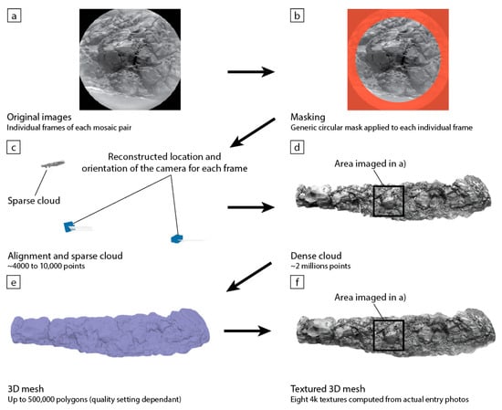
Figure 4.
Processing chain for the computation of a remote DOM from the long-distance RMI mosaics. (a) Import of raw individual frames of each mosaic. (b) Application of a generic circular mask to prevent black and overexposed/blurred areas from being considered by the software. (c) Initial alignment of the cameras and generation of a preliminary sparse point cloud. (d) Generation of dense point cloud. At this step, the actual shape of the outcrop is well recognizable. (e) Generation of a solid 3D mesh from the dense cloud. (f) Computation of a photorealistic texture from the entry images and application to the 3D mesh.
As the RMI optics provide a circular field of view recorded by a square detector matrix, a generic circular mask is applied within the photogrammetric software to all entry images (Figure 4a). This mask (red area in Figure 4b) indicates that this part of the image should not be considered during the alignment and reconstruction process. In some cases, a small amount of stray light may cause the outer border of the RMI image to appear blurred and/or overexposed (cf. Figure 4a). To prevent using these altered data, this outer part of the entry image is included within the applied mask (Figure 4b).
4.2. Camera Alignment and Sparse Cloud Generation
Once each individual frame of the RMI mosaics is imported and masked, a first alignment is computed to obtain a sparse point cloud and a 3D representation of the calculated location and orientation of the original frames in a 3D space (Figure 4c). This alignment results in a cloud composed by a few thousand points (usually 4000 to 10,000, the higher, the better). This sparse cloud gives an idea of the general shape of the distant outcrop but cannot be used for further characterization in this state. Higher density of tie-points is obtained in areas where a greater number of entry images are overlapping, and consequential to the degree of overlap.
Given the distant nature of the targeted outcrops and non-optimal points of view, results at this stage may vary. If not all of the images are aligned, one or more additional iteration(s) of the alignment process can be performed until a satisfactory number of those frames are aligned and a recognizable sparse cloud obtained. However, additional iterations may still fail to produce a good alignment, or even lead to an impossibility of aligning the images. In this latter case, changing the quality setting of the software (and thus the number of tie-points), or adding Ground Control Points (GCP) markers by hand on the entry images could help in aligning the frames and creating a sparse cloud. In some cases, some outcrops just cannot be recreated in 3D due to poor imaging and/or insufficient overlap. Further work is required to propose recommendations for future acquisitions.
4.3. Dense Cloud Generation
With entry images aligned, a dense cloud can be generated. This cloud, composed of up to several millions of points (e.g., ~2 million for mesh #1, Figure 4d), gives a very precise representation of the reconstructed area. The sharpness of the 3D reconstruction is once more linked to the degree of overlapping and overall quality of the entry images but is also a function of the quality setting in the software. In the case displayed in Figure 4, we used a high precision setting in Metashape. The resolution of this dense cloud is sufficient to fulfill our scientific needs and to perform accurate characterization of the shape and structures on the outcrop.
4.4. Mesh Generation and Texturing
The next step in the photogrammetric reconstruction process is the generation of a 3D mesh. While the dense point cloud could be exported and used to perform measurements, a mesh is computed for easier handling and visual characterization, especially when associated with a photorealistic texture, providing an accurate representation of the actual geologic object.
The mesh is composed of several thousand faces or polygons (e.g., 500,000 in mesh #1, Figure 4e) representing the surface relief of the reconstructed object. These polygons can be generated either by triangulation of the dense cloud points (with each point tied to neighbors by a vertex, creating the polygons), or by computation of a depth map. Choice of either of these methods is left to the user, depending on the capacities of the SfM software.
To obtain a more accurate and realistic representation, a texture is computed for the mesh using the original entry images. In this case, a texture made from eight tiles of 4096 × 4096 pixels have been generated and UV-mapped onto the 3D mesh to obtain a photorealistic representation of the actual distant outcrop (Figure 4f). With RMI, the texture is greyscale due to the entry images being so. However, further work is planned to test if RMI frames colorized with Mastcam images using pan-sharpening [7] could be used to produce a full color texture and therefore improve the final 3D product.
Before exporting the DOM, the mesh is manually “cleaned” from any exotic or floating polygons, most being notably on the outer margins of the model [12]. The mesh can therefore be exported for visualization and share, for example in the widespread Wavefront OBJ format, associated with textures in either JPG or PNG format and accompanying MTL library file.
5. Case Studies: Reconstruction of Distant Sulfates Unit DOMs
5.1. Mesh #1 (LD_Sulfates_2947b-2962a)
Mesh #1 is the 3D reconstruction of an area imaged by RMI targets labelled LD_Sulfates_2947b and LD_Sulfates_2962a (Table 2, Figure 5a), that represents a blocky outcrop of cross-stratified sandstones of the lower sulfate unit, which has likely undergone important diagenetic processes. The DOM was reconstructed using 41 aligned images (out of 43 in total, ~95%), taken from two points of view separated by a virtual baseline of approximately 200 m (Figure 3a, Table 2). The resulting mesh is computed from a 2,264,005 points dense cloud, into a 452,976 polygons mesh (Figure 5b). The blocky expression of the outcrop is well reconstructed by the 3D mesh, as observed in the shaded model in Figure 5b. The model is textured by eight tiles of 4096 × 4096 pixels (Figure 5c). Scaling of the resulting mesh has been done by visual comparison and selection of GCPs against scaled and calibrated original 2D RMI and Mastcam mosaics (their scale being determined as a function of the pixel size and distance to the outcrop [7,21]). We also used orbital HiRISE orthoimage to better constrain the regional coverage, resulting in a sub-metric magnitude of error, which is similar to what is observed on 2D mosaics. The resulting mesh can be visualized on the Sketchfab online public repository at: https://skfb.ly/opAwH, accessed on 5 October 2021.
Table 2.
List of targets used to compute 3D DOM of remote outcrops and associated data.
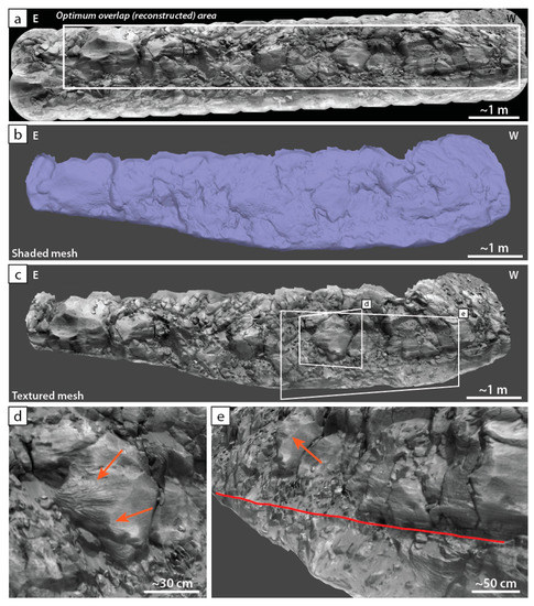
Figure 5.
Mesh #1, DOM for the target LD_Sulfates_2962a. (a) Original RMI mosaic (LD_Sulfates_2962a, ccam04962). The white box indicates the optimum overlap with associated mosaic LD_Sulfates_2947. (b) Resulting 3D mesh in shaded view, highlighting the surface relief. (c) Same view with a photorealistic texture applied. (d) Detail on a specific block reconstructed in the DOM. Orange arrows highlight the presence and distribution of probable diagenetic mineral veins. (e) Detail on the lower right part of the DOM, highlighting a topographic step (red line) corresponding to a possible continuation of the sharp contact between two sedimentary beds. The orange arrow also points to features illustrated in (d).
Thanks to the 3D reconstruction of the model, it is possible to see that sub-metric cross-stratification is quite widespread on the outcrop, and not affected by the several deflation surfaces. This area also presents some structures in the form of arcuate lineations protruding out of some blocks (orange arrows in Figure 5d,e). Here, the 3D mesh representation allows observation of the spatial distribution of these features, and they seem to crosscut the apparent stratal pattern of the entire outcrop. These structures might be interpreted as mineral veins likely of diagenetic origin. A close observation of the topographic expression of the outcrop rendered in 3D allows the viewer to identify the possibility that a contact, hardly seen on the mosaic, continues farther to the left. Indeed, the contact observed at the base of the right part of the outcrop is easily identifiable at the base of the biggest blocks (right Figure 5a,d). However, its continuity is more difficult to assess in the rubblier part on the left. The 3D mesh, however, lets us observe a topographic “step” in this rubblier part (as seen in differential shading in Figure 5b), allowing the viewer to trace the continuity of this contact down to the limits of the model (red line in Figure 5d).
5.2. Mesh #2 (LD_Sulfates_2962b-2979)
Mesh #2 is a 3D reconstruction of an area imaged by RMI targets LD_Sulfates_2962b and LD_Sulfates_2979a (Table 2, Figure 6a), that represents a hummocky outcrop of large-scale cross-stratified sandstones of the lower sulfates unit, possibly remnant of a fossilized dune field. The DOM was reconstructed using 64 aligned images (out of 73 in total, ~88%). Most non-aligned images are out of the optimum overlap area (see Figure 6a) and therefore cannot possibly be aligned as they are singletons, that is images of an object taken from an only point of view. The images were taken from two points of view separated by a virtual baseline of approximately 175 m (Figure 3a, Table 2). The resulting mesh is computed from an 836,381 points dense cloud, into a 180,000 polygons mesh (Figure 6b). The overall hummocky expression of the outcrop is well reconstructed by the 3D mesh, as observed in the shaded model in Figure 6b, despite the lack of marked relief in this specific area. The model is textured by eight tiles of 4096 × 4096 pixels (Figure 6c). The same scaling as described in Section 5.1 is applied for this mesh. The resulting mesh can be visualized on the Sketchfab online public repository at: https://skfb.ly/opAwI, accessed on 5 October 2021.
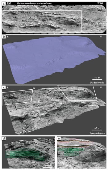
Figure 6.
Mesh #2, DOM for the target LD_Sulfates_2962b. (a) Original RMI mosaic (LD_Sulfates_2962b, ccam05962). The white box indicates the optimum overlap with associated mosaic LD_Sulfates_2979a. (b) Resulting 3D mesh in shaded view, highlighting the surface relief. (c) Same view but with photorealistic texture applied. (d) Detail on a specific small butte presenting several sets of well-evidenced cross-stratifications (green lines). (e) Detail on another small butte also evidencing well-developed cross-stratifications, but also showing two marked sharp contacts defining a deflation (bounding?) surface (red lines).
By observing the model, it is possible to see that metric-scale cross-stratifications are visible all over the outcrop (Figure 6c). Most buttes are made of those cross-stratified sandstones, and the 3D model here helps in characterizing these structures and their spatial distribution from different points of view. For example, the green line-drawing on Figure 6d,e helps identify several sets of large meter-scale sets of through cross-stratifications with their top truncated, which is common in aeolian settings. The direction of propagation implied by trough cross-stratifications is difficult to assess in simple plan/section view, therefore the different points of view permitted by the 3D DOM helps in determining the transport direction which appears to be roughly north-eastwards (Figure 6). The 3D representation also allows identification of several erosional surfaces truncating the cross-stratified structures (red line in Figure 6e), helping to decipher local bounding surfaces within this probable aeolian context.
6. Conclusions and Perspectives
While critical to understanding the sedimentary dynamics, assessing the 3D shape of the sedimentary structures in the Gale crater might be difficult relying only on 2D imagery, even of high quality. SfM photogrammetry has been recently used to propose high-resolution DOM of several areas studied by Curiosity [12,18,32,33], but these only concern outcrops that have been “physically” traversed by the rover. Many remote areas that are not accessible or not yet reached by the rover remain poorly documented in terms of 3D information. This is notably the case for the lower sulfates unit, which has been only characterized so far using orbital data [9] or observed from remote points of view using the rover’s M-100 and RMI telescope [8,11]. Still, this 3D information could be critical in helping us characterize with higher precision the sedimentary record we are observing from a distance, with higher resolution and detail than in usual orbital digital elevation models.
In this work we therefore tested the possibility of recreating the 3D shape of distant outcrop by using long-distance images obtained with the RMI telescope of Curiosity. Even if RMI was not specifically designed for long distance stereo imaging, it is the most powerful imager in terms of pixel size. We demonstrate for the first time that individual frames from overlapping long-distance RMI mosaics can be used to successfully compute DOMs of these distant outcrops on two test cases using SfM photogrammetry (performed by the Metashape software). To maximize the variation in point of view, we are using a “virtual baseline” implied by successive stops of the rover along its traverse, separated by several hundred meters.
The resulting models computed from these RMI mosaics allow examination of the overall accurate 3D shape of the geologic objects that are out of the rover’s reach. With such 3D visualization enabling a multi-point of view observation, it is therefore possible to remotely assess several critical features of the outcrops such as the transport direction represented by cross-stratified sedimentary structures, or the spatial distribution of diagenetic features with an unprecedented accuracy. Coupled with existing imagery such as Mastcam (stereo-)mosaics and usual RMI mosaics, this new original yet powerful way to characterize the 3D geological record remotely observed from several hundred meters will help the science team to characterize, for example, the distant sulfates unit of Mount Sharp, a key-objective of the MSL mission. The possibility of computing a DOM from afar with RMI could also serve to help planning the upcoming exploration of this sulfates interval before arrival of the rover on site to maximize the science return and designate high-interest targets in advance. A further evolution of this technique would be to use RMI frames that have been previously colorized using Mastcam color mosaics [7]. Adding color information to the DOM would be an important improvement that would help better characterization and understanding of the recreated structures. Finally, considering the similarity between ChemCam’s RMI and the enhanced SuperCam’s RMI aboard the newly arrived on Mars Perseverance rover [35,36,37], we could foresee a similar use to compute long-distance DOM of structures observed from the floor of the Jezero crater.
Author Contributions
Conceptualization, methodology, G.C. and S.L.M.; data planification and acquisition, G.C., S.L.M., W.R., A.F., O.G. and H.E.N.; software, G.C.; validation, W.R., G.D. and L.L.D.; writing—original draft preparation, review, and editing, G.C.; supervision, N.M. and O.G.; project administration, funding acquisition, O.G., S.M., R.C.W. and N.L.L. All authors have read and agreed to the published version of the manuscript.
Funding
This work was supported by NASA’s Mars Exploration Program in the US under NASA contract NNH13ZDA018O to LANL, and by CNES in France under convention CNES 180027.
Institutional Review Board Statement
Not applicable.
Informed Consent Statement
Not applicable.
Data Availability Statement
All Mars Science Laboratory data are freely accessible to the public. Raw RMI images can be accessed on the Jet Propulsion Laboratory’s raw images archive at: https://mars.nasa.gov/msl/multimedia/raw-images/, accessed on 5 October 2021. RMI images can also be accessed on the Planetary Data System database at: pds-geosciences.wustl.edu/msl/msl-m-chemcam-libs-4_5-rdr-v1/mslccm_1xxx/data/, accessed on 5 October 2021. Preprocessed mosaics made from individual RMI images can be accessed on the Planetary Data System database at: https://pds-geosciences.wustl.edu/msl/msl-m-chemcam-libs-4_5-rdr-v1/mslccm_1xxx/extras/rmi_mosaics/, accessed on 5 October 2021. All 3D models discussed in this article are freely accessible and visualizable on the public Sketchfab web platform.
Acknowledgments
The authors thank all the people from the MSL and ChemCam teams that made these observations possible. We also thank four anonymous reviewers for their constructive inputs.
Conflicts of Interest
The authors declare no conflict of interest.
References
- Grotzinger, J.P.; Sumner, D.Y.; Kah, L.C.; Stack, K.; Gupta, S.; Edgar, L.; Rubin, D.; Lewis, K.; Schieber, J.; Mangold, N.; et al. A Habitable Fluvio-Lacustrine Environment at Yellowknife Bay, Gale Crater, Mars. Science 2014, 343, 1242777. [Google Scholar] [CrossRef]
- Grotzinger, J.; Gupta, S.; Malin, M.; Rubin, D.; Schieber, J.; Siebach, K.; Sumner, D.; Stack, K.; Vasavada, A.; Arvidson, R.; et al. Deposition, exhumation, and paleoclimate of an ancient lake deposit, Gale crater, Mars. Science 2015, 350, aac7575. [Google Scholar] [CrossRef]
- Maki, J.; Thiessen, D.; Pourangi, A.; Kobzeff, P.; Litwin, T.; Scherr, L.; Elliott, S.; Dingizian, A.; Mainome, M. The Mars Science Laboratory Engineering Cameras. Space Sci. Rev. 2012, 170, 77–93. [Google Scholar] [CrossRef]
- Malin, M.C.; Caplinger, M.A.; Edgett, K.S.; Ghaemi, F.T.; Ravine, M.A.; Schaffner, J.A.; Baker, J.M.; Bardis, J.D.; Dibiase, D.R.; Maki, J.N.; et al. The Mars Science Laboratory (MSL) Mast-mounted Cameras (Mastcams) Flight Instruments. In Proceedings of the 41st Lunar and Planetary Science Conference, The Woodlands, TX, USA, 1–5 March 2010; Abstract #1123. Available online: https://www.lpi.usra.edu/meetings/lpsc2010/pdf/1123.pdf (accessed on 8 August 2021).
- Bell III, J.F.; Godber, A.; Rice, M.S.; Fraeman, A.A.; Ehlmann, B.L.; Goetz, W.; Hardgrove, C.J.; Harker, D.E.; Johnson, J.R.; Kinch, K.M.; et al. Initial multispectral imaging results from the Mars Science Laboratory Mastcam investigation at the Gale crater field site. In Proceedings of the 44th Lunar and Planetary Science Conference, The Woodlands, TX, USA, 18–22 March 2013; Abstract #1719. Available online: https://www.lpi.usra.edu/meetings/lpsc2013/pdf/1417.pdf (accessed on 8 August 2021).
- Maurice, S.; Wiens, R.C.; Saccoccio, M.; Barraclough, B.; Gasnault, O.; Forni, O.; Mangold, N.; Baratoux, D.; Bender, S.; Berger, G.; et al. The ChemCam instrument suite on the Mars Science Laboratory (MSL) rover: Science objectives and mast unit description. Space Sci. Rev. 2012, 170, 95–166. [Google Scholar] [CrossRef]
- Le Mouélic, S.; Gasnault, O.; Herkenhoff, K.E.; Bridges, N.T.; Langevin, Y.; Mangold, N.; Maurice, S.; Wiens, R.C.; Pinet, P.; Newsom, H.E.; et al. The ChemCam Remote Micro-Imager at Gale Crater: Review of the first year of operation on Mars. Icarus 2015, 249, 93–107. [Google Scholar] [CrossRef]
- Le Deit, L.; Anderson, R.B.; Le Mouélic, S.; Mangold, N.; Dromart, G.; Maurice, S.; Gasnault, O.; Wiens, R.C. Lower Mount Sharp, Gale crater, Mars: Key study areas as observed by Curiosity remote cameras. In Proceedings of the 49th Lunar and Planetary Science Conference, The Woodlands, TX, USA, 19–23 March 2018; Abstract #1437. Available online: https://www.hou.usra.edu/meetings/lpsc2018/pdf/1437.pdf (accessed on 8 August 2021).
- Milliken, R.E.; Grotzinger, J.P.; Thomson, B.J. Paleoclimate of Mars as captured by the stratigraphic record in Gale Crater. Geophys. Res. Let. 2010, 37. [Google Scholar] [CrossRef] [Green Version]
- Fraeman, A.A.; Ehlmann, B.L.; Arvidson, R.E.; Edwards, C.S.; Grotzinger, J.P.; Milliken, R.E.; Quinn, D.P.; Rice, M.S. The stratigraphy and evolution of lower Mount Sharp from spectral, morphological, and thermophysical orbital data sets. J. Geophys. Res. Planets 2016, 121, 1713–1736. [Google Scholar] [CrossRef] [PubMed]
- Rapin, W.; Dromart, G.; Rubin, D.; Le Deit, L.; Mangold, N.; Edgar, L.A.A.; Gasnault, O.; Herkenhoff, K.; Le Mouélic, S.; Anderson, R.B.; et al. Alternating wet and dry depositional environments recorded in the stratigraphy of Mount Sharp at Gale crater, Mars. Geology 2021, 49, 842–846. [Google Scholar] [CrossRef]
- Caravaca, G.; Le Mouélic, S.; Mangold, N.; L’Haridon, J.; Le Deit, L.; Massé, M. 3D digital outcrop model reconstruction of the Kimberley outcrop (Gale crater, Mars) and its integration into Virtual Reality for simulated geological analysis. Planet. Space Sci. 2020, 182, 104808. [Google Scholar] [CrossRef]
- Mangold, N.; Forni, O.; Dromart, G.; Stack, K.; Wiens, R.C.; Gasnault, O.; Sumner, D.Y.; Nachon, M.; Meslin, P.Y.; Anderson, R.B.; et al. Chemical variations in Yellowknife Bay formation sedimentary rocks analyzed by ChemCam on board the Curiosity rover on Mars. J. Geophys. Res. Planets 2015, 120, 452–482. [Google Scholar] [CrossRef]
- Le Deit, L.; Mangold, N.; Forni, O.; Cousin, A.; Lasue, J.; Schröder, S.; Wiens, R.C.; Sumner, D.; Fabre, C.; Stack, K.M.; et al. The potassic sedimentary rocks in Gale Crater, Mars, as seen by ChemCam on board Curiosity. J. Geophys. Res. Planets 2016, 121, 784–804. [Google Scholar] [CrossRef] [Green Version]
- Stack, K.M.; Edwards, C.S.; Grotzinger, J.P.; Gupta, S.; Summer, D.Y.; Calef III, F.J.; Edgar, L.A.; Edgett, K.S.; Framan, A.A.; Jacob, S.R.; et al. Comparing orbiter and rover image-based mapping of an ancient sedimentary environment, Aeolis Palus, Gale Crater, Mars. Icarus 2016, 280, 3–21. [Google Scholar] [CrossRef] [Green Version]
- Stack, K.M.; Grotzinger, J.P.; Lamb, M.P.; Gupta, S.; Rubin, D.M.; Kah, L.C.; Edgar, L.A.; Fey, D.M.; Hurowitz, J.A.; McBride, M.; et al. Evidence for plunging river plume deposits in the Pahrump Hills member of the Murray formation, Gale crater, Mars. Sedimentology 2019, 66, 1768–1802. [Google Scholar] [CrossRef] [Green Version]
- Edgar, L.A.; Fedo, C.M.; Gupta, S.; Banham, S.G.; Fraeman, A.A.; Grotzinger, J.P.; Stack, K.M.; Stein, N.T.; Bennett, K.A.; Rivera-Hernandez, F.; et al. A lacustrine paleoenvironment recorded at Vera Rubin ridge, Gale crater: Overview of the Sedimentology and Stratigraphy observed by the Mars Science Laboratory Curiosity rover. J. Geophys. Res. Planets 2020, 125, e2019JE006307. [Google Scholar] [CrossRef] [Green Version]
- Banham, S.G.; Gupta, S.; Rubin, D.M.; Watkins, J.A.; Sumner, D.Y.; Edgett, K.S.; Grotzinger, J.P.; Lewis, K.W.; Edgar, L.A.; Stack Morgan, K.M.; et al. Ancient Martian aeolian processes and palaeomorphology reconstructed from the Stimson formation on the lower slope of Aeolis Mons, Gale crater, Mars. Sedimentology 2018, 65, 993–1042. [Google Scholar] [CrossRef] [Green Version]
- Dromart, G.; Le Deit, L.; Rapin, W.; Gasnault, O.; Le Mouélic, S.; Quantin-Nataf, C.; Mangold, N.; Rubn, D.; Lasue, J.; Maurice, S.; et al. Deposition and erosion of a Light-Toned Yardang-forming unit of Mount Sharp, Gale crater, Mars. Earth Planet. Sci. Let. 2021, 554, 116681. [Google Scholar] [CrossRef]
- Ostwald, A.; Hurtado, J. 3D models from structure-from-motion photogrammetry using Mars science laboratory images: Methods and implications. In Proceedings of the 48th Lunar and Planetary Science Conference, The Woodlands, TX, USA, 20–24 March 2017; Abstract#1787. Available online: https://www.hou.usra.edu/meetings/lpsc2017/pdf/1787.pdf (accessed on 8 August 2021).
- Malin, M.C.; Ravine, M.A.; Caplinger, M.A.; Ghaemi, F.T.; Schaffner, J.A.; Maki, J.N.; Bell III, J.F.; Cameron, J.F.; Dietrich, W.E.; Edgett, K.S.; et al. The Mars Science Laboratory (MSL) Mast cameras and Descent imager: Inverstigation and instrument description. Earth Space Sci. 2017, 4, 506–539. [Google Scholar] [CrossRef] [PubMed] [Green Version]
- Wiens, R.; Maurice, S.; Barraclough, B.; Saccoccio, M.; Barkley, W.C.; Bell, J.F., III; Bender, S.; Bernardin, J.; Blaney, D.; Blank, J.; et al. The ChemCam Instrument Suite on the Mars Science Laboratory (MSL) Rover: Body Unit and Combined System Tests. Space Sci. Rev. 2012, 170, 167–227. [Google Scholar] [CrossRef]
- Le Mouélic, S.; Gasnault, O.; Rapin, W.; Bryk, A.B.; Dietriech, W.E.; Dromart, G.; Wiens, R.C.; Caravaca, G.; Mangold, N.; Newson, H.; et al. Housedon Hill—A ChemCam RMI mega mosaic to investigate distant features in Gale crater. In Proceedings of the 52nd Lunar and Planetary Science Conference, Virtual Conference, 15–19 March 2021; Abstract #1408. Available online: https://www.hou.usra.edu/meetings/lpsc2021/pdf/1408.pdf (accessed on 8 August 2021).
- Ullman, S. The interpretation of structure from motion. Proc. R. Soc. Lond. Ser. B Biol. Sci. 1979, 203, 405–426. [Google Scholar] [CrossRef]
- Verhoeven, G. Taking computer vision aloft–archaeological three-dimensional reconstructions from aerial photographs with photoscan. Archaeol. Prospect. 2011, 18, 67–73. [Google Scholar] [CrossRef]
- Arbuées, P.; García-Sellés, D.; Granado, P.; Lopez-Blanco, M.; Muñoz, J. A method for producing photorealistic digital outcrop models. In Proceedings of the 74th EAGE Conference and Exhibition Incorporating EUROPEC, Abstract #D029, Copenhagen, Denmark, 4–7 June 2012. [Google Scholar] [CrossRef]
- Tavani, S.; Granado, P.; Corradetti, A.; Girundo, M.; Iannace, A.; Arbués, P.; Muñoz, J.A.; Mazzoli, S. Building a virtual outcrop, extracting geological information from it, and sharing the results in Google Earth via OpenPlot and Photoscan: An example from the Khaviz Anticline (Iran). Comput. Geosci. 2014, 63, 44–53. [Google Scholar] [CrossRef]
- Triantafyllou, A.; Watlet, A.; Le Mouélic, S.; Camelbeeck, T.; Civet, F.; Kaufmann, O.; Quinif, Y.; Vandycke, S. 3-D digital outcrop model for analysis of brittle deformation and lithological mapping (Lorette cave, Belgium). J. Struct. Geol. 2019, 120, 55–66. [Google Scholar] [CrossRef]
- Nesbit, P.R.; Boulding, A.D.; Hugenholtz, C.H.; Durkin, P.R.; Hubbard, S.M. Visualization and Sharing of 3D Digital Outcrop Models to Promote Open Science. GSA Today 2020, 30, 4–10. [Google Scholar] [CrossRef] [Green Version]
- Barnes, R.; Gupta, S.; Traxler, C.; Ortner, T.; Bauer, A.; Hesina, G.; Paar, G.; Huber, B.; Juhart, K.; Fritz, L.; et al. Geological analysis of Martian rover-derived Digital Outcrop Models using the 3-D visualization tool, Planetary Robotics 3-D Viewer-PRo3D. Earth Space Sci. 2018, 5, 285–307. [Google Scholar] [CrossRef]
- Le Mouélic, S.; Enguehard, P.; Schmitt, H.H.; Caravaca, G.; Seignovert, B.; Mangold, N.; Combe, J.-P.; Civet, F. Investigating lunar boulders at the Apollo 17 landing site using photogrammetry and Virtual Reality. Remote Sens. 2020, 12, 1900. [Google Scholar] [CrossRef]
- Caravaca, G.; Mangold, N.; Dehouck, E.; Schieber, J.; Bryk, A.B.; Fedo, C.M.; Le Mouélic, S.; Banham, S.G.; Gupta, S.; Cousin, A.; et al. Evidence of depositional settings variation at the Jura/Knockfarril Hill members transition in the Glen Torridon region (Gale crater, Mars). In Proceedings of the 52nd Lunar and Planetary Science Conference, Virtual Conference, 15–19 March 2021; Abstract #1455. Available online: https://www.hou.usra.edu/meetings/lpsc2021/pdf/1455.pdf (accessed on 8 August 2021).
- De Toffoli, B.; Mangold, N.; Massironi, M.; Zanella, A.; Pozzobon, R.; Le Mouélic, S.; L’Haridon, J.; Cremonese, G. Structural analysis of sulfate vein networks in Gale crater (Mars). J. Struct. Geol. 2020, 137, 104083. [Google Scholar] [CrossRef]
- Agisoft LLC. Metashape Professional v.1.7.x. 2021. Available online: https://www.agisoft.com (accessed on 15 June 2021).
- Wiens, R.C.; Maurice, S.; Robinson, S.H.; Nelson, A.E.; Cais, P.; Bernardi, P.; Newell, R.T.; Clegg, S.; Sharma, S.K.; Storms, S.; et al. The SuperCam instrument suite on the NASA Mars 2020 rover: Body unit and Combined system tests. Space Sci. Rev. 2020, 217, 4. [Google Scholar] [CrossRef]
- Gasnault, O.; Virmontois, C.; Maurice, S.; Wiens, R.C.; Le Mouélic, S.; Bernardi, P.; Forni, O.; Pilleri, P.; Daydou, Y.; Rapin, W.; et al. What SuperCam will see: The Remote Micro-Imager aboard Perseverance. In Proceedings of the 52nd Lunar and Planetary Science Conference, Virtual Conference, 15–19 March 2021; Abstract #2248. Available online: https://www.hou.usra.edu/meetings/lpsc2021/pdf/2248.pdf (accessed on 8 August 2021).
- Maurice, S.; Wiens, R.C.; Bernardi, P.; Caïs, P.; Robinson, S.; Nelson, T.; Gasnault, O.; Reess, J.-M.; Deleuze, M.; Rull, F.; et al. The SuperCam Instrument suite on the Mars 2020 rover: Science objectives and Mast-unit description. Space Sci. Rev. 2021, 217, 47. [Google Scholar] [CrossRef]
Publisher’s Note: MDPI stays neutral with regard to jurisdictional claims in published maps and institutional affiliations. |
© 2021 by the authors. Licensee MDPI, Basel, Switzerland. This article is an open access article distributed under the terms and conditions of the Creative Commons Attribution (CC BY) license (https://creativecommons.org/licenses/by/4.0/).