
Three-Dimensional Convolutional Neural Network Model for Early Detection of Pine Wilt Disease Using UAV-Based Hyperspectral Images

 ,
,  ,
,  ,
, 
Abstract
:1. Introduction
2. Materials and Methods
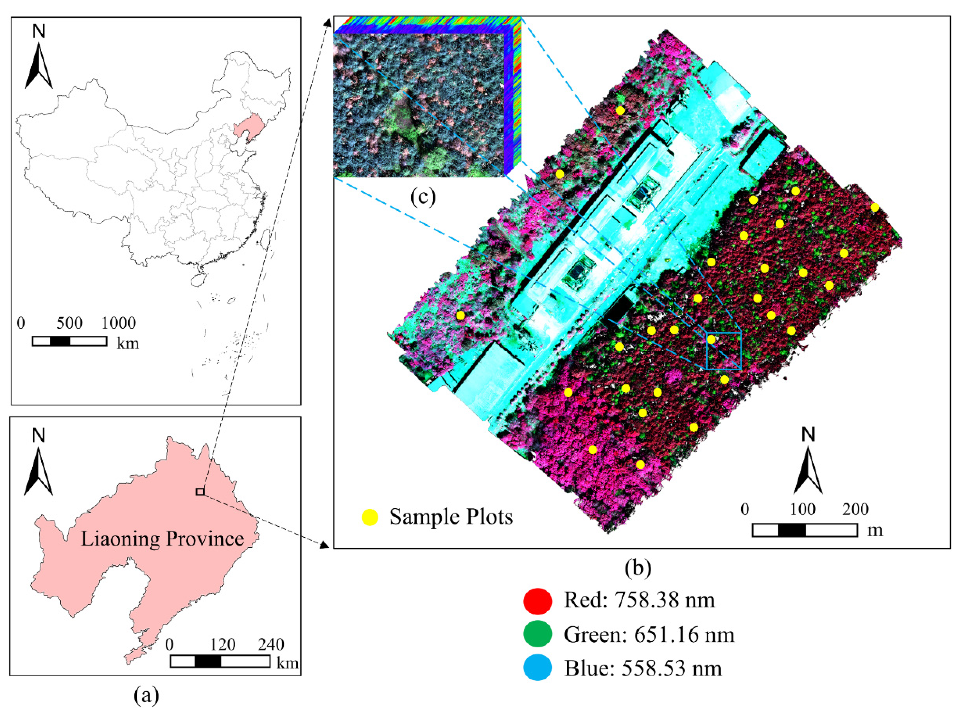
2.1. Study Area and Ground Survey
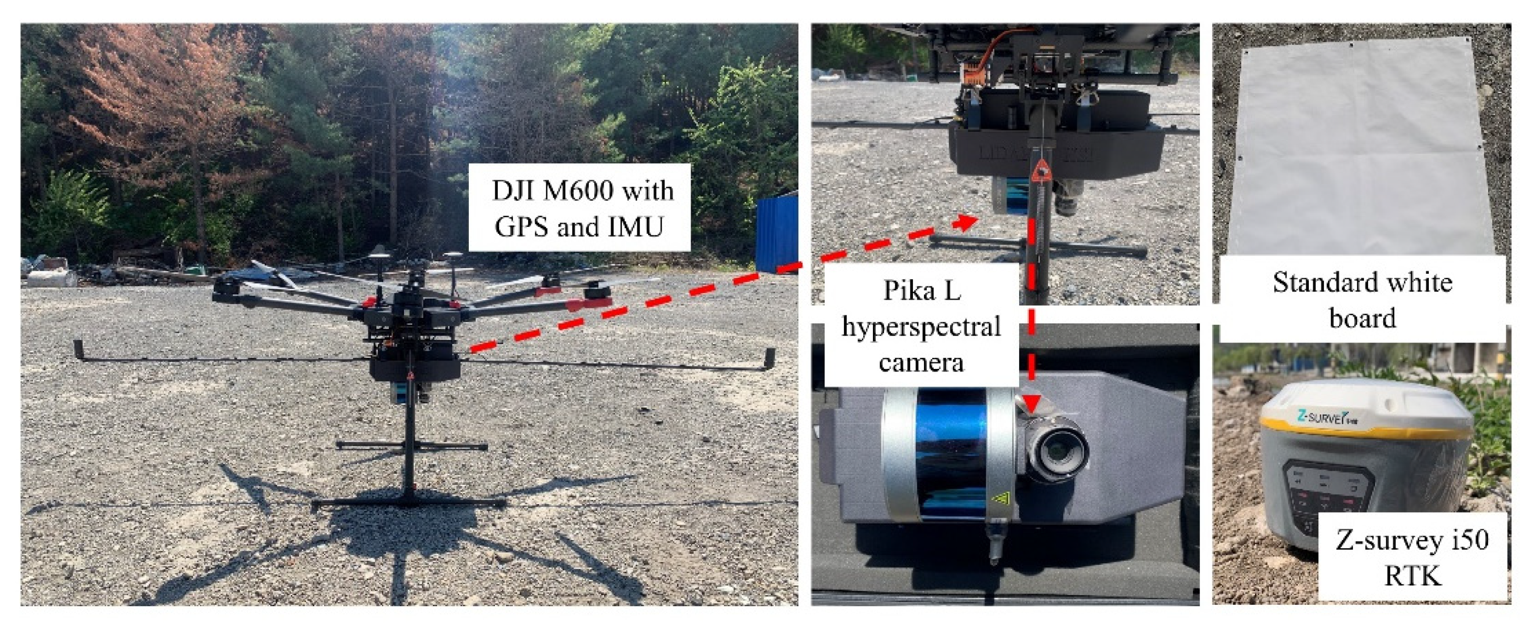
2.2. Airborne Data Collection and Preprocessing
2.3. Division of PWD Infection Stage and Data Labeling
2.4. Model Construction
2.4.1. 3D-CNN
2.4.2. Construction of the 3D-Res CNN Classification Model
- (1)
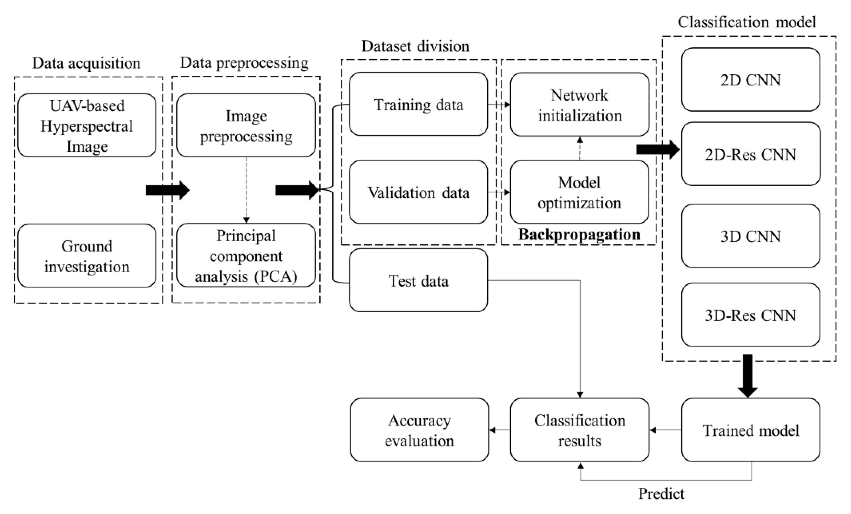
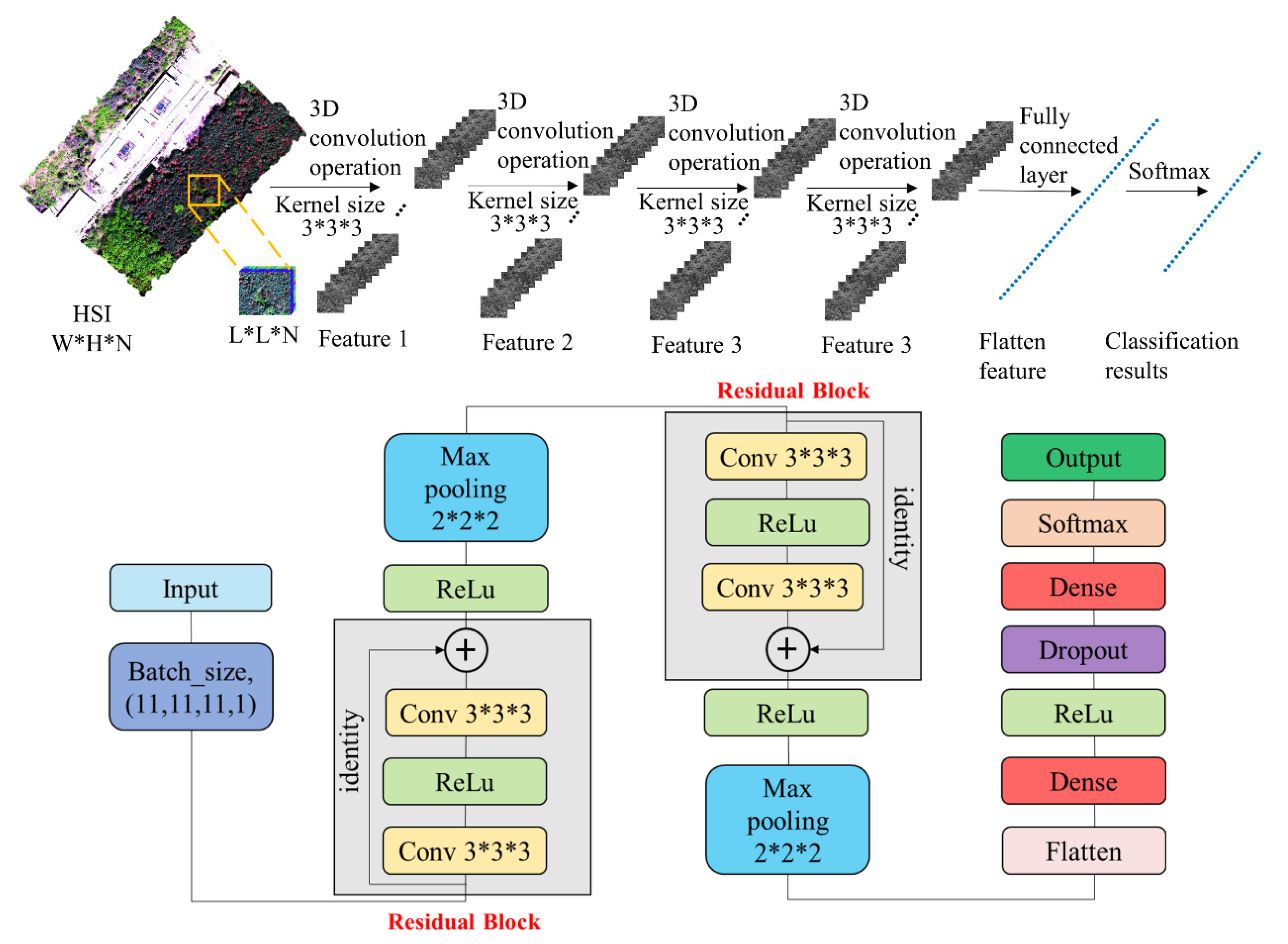
- Data collection from HI. Here, 3D-CNN can use raw data without dimensionality reduction or feature filtering, but the data collected in this study were enormous and contained a lot of redundant information. Therefore, to make our model more rapid and lightweight, the dimensionality of the raw data was reduced through a principal component analysis (PCA), and 11 principal components (PCs) were extracted for further analyses. The objective pixel was set as the center, and the spatial-spectral cubes with a size of L × L × N as well as their category information were extracted. Here, L × L stands for the space size, and N is the number of bands in the image.
- (2)
- Feature extraction after 3-D convolution operation. The model includes four convolution layers and two fully connected layers. The spatial-spectral cubes (L × L × N) obtained from the previous step were used as input of the model. The first convolutional layer (Conv1) contains 32 convolution kernels with a size of 3 × 3 × 3, a step size of 1 × 1 × 1, and a padding of 1. The 32 output 3-D cubes (cubes-Conv1) had a size of (L—kernel size + 2 × padding)/stride + 1. The 32 cubes-Conv1 were input to the second convolution layer (Conv2), and 32 output 3-D cubes (cubes-Conv2) were obtained. The add operation was performed on the output of the input and cubes-Conv2, and the activation function and pooling layer (k = 2 × 2 × 2, stride = 2 × 2 × 2) were applied for down-sampling. As a result, the length, width, and height of these cubes were reduced to half of the original values; the 32 output 3-D cubes were denoted as cubes-Pool1. After two more rounds of convolution operation, cubes-Conv4 were obtained; the add operation was performed to cubes-Pool1 and cubes-Conv4. After applying the activation function and the pooling layer, the length, width, and height were again reduced to half of the original values, and the 32 output cubes were denoted as cubes-Pool2.
- (3)
- Residual blocks. The residual structure consists of two convolution layers. The data were input to the first convolution layer (Conv1R), and the rectified linear unit (ReLU) activation function was used. The output of Conv1R was input to the second convolution layer (Conv2R), and the ReLU activation function was used to obtain the output of Conv2R. The add operation was performed on the output of Conv1R and Conv2R, and the ReLU activation function was then employed to obtain the output of the whole residual structure.
- (4)
- Fully connected layers. The features of cubes-Pool2 were flattened, and by applying the fully connected layers, the cubes-Pool2 were transformed into feature vectors with a size of 1 × 128.
- (5)
- Logistic regression. A logistic regression classifier was added after the fully connected layers. Softmax was applied for multiple classification. After flattening the features of the input data, the probability of these features can be attached to each category of trees.
2.5. Comparison between the 3D-Res CNN and Other Models
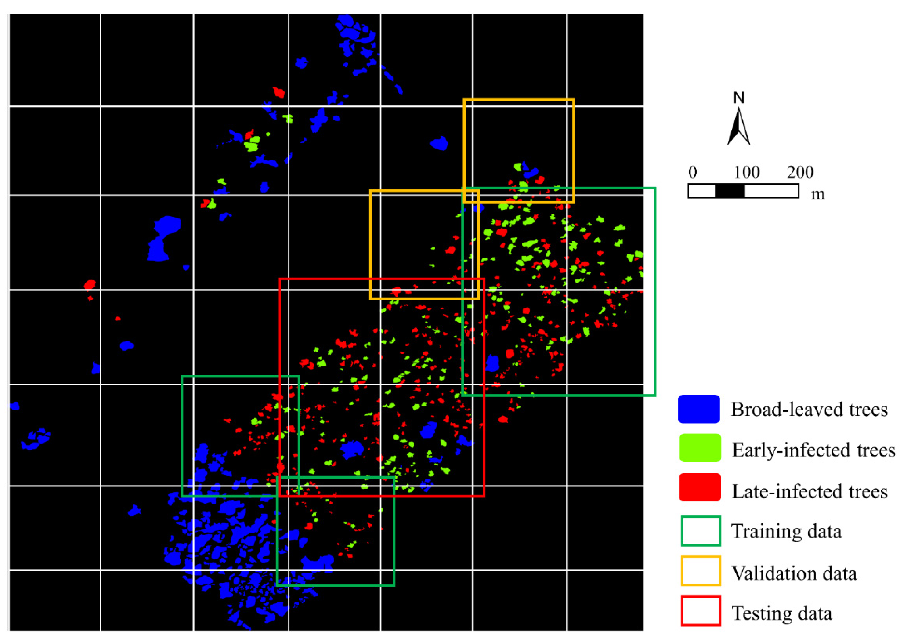
2.6. Dataset Division and Evaluation Metrics
3. Results
4. Discussion
4.1. Comparison of Different Models and the Contribution of Residual Learning
4.2. Early Monitoring of PWD
4.3. Existing Deficiencies and Future Prospects
5. Conclusions
Author Contributions
Funding
Institutional Review Board Statement
Informed Consent Statement
Data Availability Statement
Acknowledgments
Conflicts of Interest
References
- Mamiya, Y.; Kiyohara, T. Description of Bursaphelenchus Lignicolus N. Sp. (Nematoda: Aphelenchoididae) from pine wood and histopathology of nematode-infested trees. Nematologica 1972, 18, 120–124. [Google Scholar] [CrossRef]
- Rodrigues, M. National Eradication Programme for the Pinewood Nematode. In PineWilt Disease: AWorldwide Threat to Forest Ecosystems; Mota, M.M., Vieira, P., Eds.; Springer: Kato Bunmeisha, Japan, 2008; pp. 5–14. [Google Scholar]
- Robertson, L.; Cobacho Arcos, S.; Escuer, M.; Santiago Merino, R.; Esparrago, G.; Abelleira, A.; Navas, A. Incidence of the pinewood nematode Bursaphelenchus xylophlius Steiner & Buhrer, 1934 (Nickle, 1970) in Spain. Nematology 2011, 13, 755–757. [Google Scholar]
- Fonseca, L.; Santos, M.; Santos, M.; Curtis, R.; Abrantes, I. Morpho-biometrical characterization of Portuguese Bursaphelenchus xylophilus isolates with mucronate, digitate or round tailed females. Phytopathol. Mediterr. 2009, 47, 223–2334. [Google Scholar]
- Ye, J. Epidemic status of pine wilt disease in China and its prevention and control techniques and counter measures. Sci. Silv. Sin. 2019, 55, 1–10. [Google Scholar]
- Togashi, K.; Arakawa, Y. Horizontal Transmission of Bursaphelenchus xylophilus between Sexes of Monochamus alternatus. J. Nematol. 2003, 35, 7–16. [Google Scholar] [PubMed]
- Kobayashi, F.; Yamane, A.; Ikeda, T. The Japanese pine sawyer beetle as the vector of pine wilt disease. Annu. Rev. Entomol. 2003, 29, 115–135. [Google Scholar] [CrossRef]
- Mamiya, Y. Pathology of the pine wilt disease caused by Bursaphelenchus xylophilus. Annu. Rev. Phytopathol. 1983, 21, 201–220. [Google Scholar] [CrossRef] [PubMed]
- Yu, H.; Wu, H.; Zhang, X.; Wang, L.; Zhang, X.; Song, Y. Preliminary study on Larix spp. infected by Bursaphelenchus xylophilus in natural environment. For. Pest Dis. 2019, 38, 7–10. [Google Scholar]
- Pan, L.; Li, Y.; Liu, Z.; Meng, F.; Chen, J.; Zhang, X. Isolation and identification of pine wood nematode in Pinus koraiensis in Fengcheng, Liaoning Province. For. Pest Dis. 2019, 38, 1–4. [Google Scholar]
- Yu, R.; Ren, L.; Luo, Y. Early detection of pine wilt disease in Pinus tabuliformis in North China using a field portable spectrometer and UAV-based hyperspectral imagery. For. Ecosyst. 2021, 8, 44. [Google Scholar] [CrossRef]
- Lin, X. Review on damage and control measures of pine wilt disease. East China For. Manag. 2015, 29, 28–30. [Google Scholar]
- Allen, C.D.; Breshears, D.D.; McDowell, N.G. On underestimation of global vulnerability to tree mortality and forest die-off from hotter drought in the Anthropocene. Ecosphere 2015, 6, 1–55. [Google Scholar] [CrossRef]
- Wong, C.M.; Daniels, L.D. Novel forest decline triggered by multiple interactions among climate, an introduced pathogen and bark beetles. Glob. Chang. Biol. 2017, 23, 1926–1941. [Google Scholar] [CrossRef] [PubMed] [Green Version]
- Kärvemo, S.; Johansson, V.; Schroeder, M.; Ranius, T. Local colonization-extinction dynamics of a tree-killing bark beetle during a large-scale outbreak. Ecosphere 2016, 7, e01257. [Google Scholar] [CrossRef] [Green Version]
- Umebayashi, T.; Yamada, T.; Fukuhara, K.; Endo, R.; Kusumoto, D.; Fukuda, K. In situ observation of pinewood nematode in wood. Eur. J. Plant Pathol. 2017, 147, 463–467. [Google Scholar] [CrossRef]
- Kim, S.-R.; Lee, W.-K.; Lim, C.-H.; Kim, M.; Kafatos, M.; Lee, S.-H.; Lee, S.-S. Hyperspectral analysis of pine wilt disease to determine an optimal detection index. Forests 2018, 9, 115. [Google Scholar] [CrossRef] [Green Version]
- Iordache, M.-D.; Mantas, V.; Baltazar, E.; Pauly, K.; Lewyckyj, N. A machine learning approach to detecting pine wilt disease using airborne spectral imagery. Remote Sens. 2020, 12, 2280. [Google Scholar] [CrossRef]
- Wu, B.; Liang, A.; Zhang, H.; Zhu, T.; Zou, Z.; Yang, D.; Tang, W.; Li, J.; Su, J. Application of conventional UAV-based high-throughput object detection to the early diagnosis of pine wilt disease by deep learning. For. Ecol. Manag. 2021, 486, 118986. [Google Scholar] [CrossRef]
- Yu, R.; Luo, Y.; Zhou, Q.; Zhang, X.; Ren, L. Early detection of pine wilt disease using deep learning algorithms and UAV-based multispectral imagery. For. Ecol. Manag. 2021, 497, 119493. [Google Scholar] [CrossRef]
- Mäyrä, J.; Keski-Saari, S.; Kivinen, S.; Tanhuanpää, T.; Hurskainen, P.; Kullberg, P.; Poikolainen, L.; Viinikka, A.; Tuominen, S.; Kumpula, T.; et al. Tree species classification from airborne hyperspectral and lidar data using 3D convolutional neural networks. Remote Sens. Environ. 2021, 256, 112322. [Google Scholar] [CrossRef]
- Mou, L.; Ghamisi, P.; Zhu, X.X. Deep recurrent neural networks for hyperspectral image classification. IEEE Trans. Geosci. Remote Sens. 2017, 55, 3639–3655. [Google Scholar] [CrossRef] [Green Version]
- LeCun, Y.; Bengio, Y.; Hinton, G. Deep Learning. Nature 2015, 521, 436–444. [Google Scholar] [CrossRef]
- Zhang, B.; Zhao, L.; Zhang, X. Three-dimensional convolutional neural network model for tree species classification using airborne hyperspectral images. Remote Sens. Environ. 2020, 247, 111938. [Google Scholar] [CrossRef]
- Hinton, G.; Salakhutdinov, R. Reducing the dimensionality of data with neural networks. Science 2006, 313, 504–507. [Google Scholar] [CrossRef] [PubMed] [Green Version]
- Vincent, P.; Larochelle, H.; Lajoie, I.; Bengio, Y.; Manzagol, P.A.; Bottou, L. Stacked denoising autoencoders: Learning useful representations in a deep network with a local denoising criterion. J. Mach. Learn. Res. 2010, 11, 3371–3408. [Google Scholar]
- Krizhevsky, A.; Sutskever, I.; Hinton, G. Imagenet classification with deep convolutional neural networks. Adv. Neural Inf. Process. Syst. 2012, 25, 1097–1105. [Google Scholar] [CrossRef]
- Girshick, R.; Donahue, J.; Darrell, T.; Malik, J. Rich feature hierarchies for accurate object detection and semantic segmentation. In Proceedings of the IEEE conference on computer vision and pattern recognition, Columbus, OH, USA, 23–28 June 2014; pp. 580–587. [Google Scholar]
- Simonyan, K.; Zisserman, A. Very Deep Convolutional Networks for Large-Scale Image Recognition. arXiv 2014, arXiv:1409.1556. [Google Scholar]
- Szegedy, C.; Liu, W.; Jia, Y.; Sermanet, P.; Reed, S.; Anguelov, D.; Erhan, D.; Vanhoucke, V.; Rabinovich, A. Going deeper with convolutions. In Proceedings of the IEEE Conference on Computer Vision and Pattern Recognition, Boston, MA, USA, 7–12 June 2015; pp. 1–9. [Google Scholar]
- Qin, J.; Wang, B.; Wu, Y.; Lu, Q.; Zhu, H. Identifying Pine Wood Nematode Disease Using UAV Images and Deep Learning Algorithms. Remote Sens. 2021, 13, 162. [Google Scholar] [CrossRef]
- Tao, H.; Li, C.; Zhao, D.; Deng, S.; Jing, W. Deep learning-based dead pine trees detection from unmanned aerial vehicle images. Int. J. Remote Sens. 2020, 41, 8238–8255. [Google Scholar] [CrossRef]
- Chen, Y.; Jiang, H.; Li, C.; Jia, X.; Ghamisi, P. Deep Feature Extraction and Classification of Hyperspectral Images Based on Convolutional Neural Networks. IEEE Trans. Geosci. Remote Sens. 2016, 54, 6232–6251. [Google Scholar] [CrossRef] [Green Version]
- He, M.; Bo, L.; Chen, H. Multi-scale 3D deep convolutional neural network for hyperspectral image classification. In Proceedings of the 2017 IEEE International Conference on Image Processing (ICIP), Beijing, China, 17–20 September 2017; pp. 3904–3908. [Google Scholar]
- Li, Y.; Zhang, H.; Shen, Q. Spectral-spatial classification of hyperspectral imagery with 3D convolutional neural network. Remote Sens. 2017, 9, 67. [Google Scholar] [CrossRef] [Green Version]
- He, K.; Zhang, X.; Ren, S.; Sun, J. Deep Residual Learning for Image Recognition. In Proceedings of the IEEE conference on computer vision and pattern recognition, Las Vegas, NV, USA, 27–30 June 2016; pp. 770–778. [Google Scholar]
- He, K.; Zhang, X.; Ren, S.; Sun, J. Identity Mappings in Deep Residual Networks. Lect. Notes Comput. Sci. 2016, 630–645. [Google Scholar] [CrossRef] [Green Version]
- Zhong, Z.; Li, J.; Luo, Z.; Chapman, M. Spectral-spatial residual network for hyperspectral image classification: A 3-D deep learning framework. IEEE Trans. Geosci. Remote Sens. 2017, 56, 847–858. [Google Scholar] [CrossRef]
- Lu, Z.; Xu, B.; Sun, L.; Zhan, T.; Tang, S. 3-D Channel and Spatial Attention Based Multiscale Spatial–Spectral Residual Network for Hyperspectral Image Classification. IEEE J. Sel. Top. Appl. Earth Obs. Remote Sens. 2020, 13, 4311–4324. [Google Scholar] [CrossRef]
- Zhao, L.; Zhang, X.; Wu, Y.; Zhang, B. Subtropical Forest Tree Species Classification Based on 3D-CNN for Airborne Hyperspectral Data. Sci. Silv. Sin. 2020, 11, 97–107. [Google Scholar]
- Gu, J.; Wang, J.; Braasch, H.; Burgermeister, W.; Schroder, T. Morphological and molecular characterization of mucronate isolates (M form) of Bursaphelenchus xylophilus (Nematoda: Aphelenchoididae). Russ. J. Nematol. 2011, 19, 103–120. [Google Scholar]
- Iwahori, H.; Futai, K. Lipid peroxidation and ion exudation of pine callus tissues inoculated with pinewood nematodes. Jpn. J. Nematol. 1993, 23, 79–89. [Google Scholar] [CrossRef]
- Ji, S.; Xu, W.; Yang, M.; Yu, K. 3D convolutional neural networks for human action recognition. IEEE Trans. Pattern Anal. Mach. Intell. 2013, 35, 221–231. [Google Scholar] [CrossRef] [Green Version]
- Tran, D.; Bourdev, L.; Fergus, R.; Torresani, L.; Paluri, M. Learning spatiotemporal features with 3D convolutional networks. In Proceedings of the IEEE International Conference on Computer Vision, Santiago, Chile, 7–13 December 2015; pp. 4489–4497. [Google Scholar]
- Hinton, G.E.; Srivastava, N.; Krizhevsky, A.; Sutskever, I.; Salakhutdinov, R.R. Improving neural networks by preventing co-adaptation of feature detectors. Comput. Sci. 2012, arXiv:1207.0580. [Google Scholar]
- Congalton, R. A review of assessing the accuracy of classification of remotely sensed data. Remote Sens. Environ. 1991, 37, 35–46. [Google Scholar] [CrossRef]
- Hao, Z.; Li, Y.; Jiang, Y. Deep learning for hyperspectral imagery classification: The state of the art and prospects. Acta Autom. Sin. 2018, 44, 961–977. [Google Scholar]
- Yu, R.; Luo, Y.; Zhou, Q.; Zhang, X.; Wu, D.; Ren, L. A machine learning algorithm to detect pine wilt disease using UAV-based hyperspectral imagery and LiDAR data at the tree level. Int. J Appl. Earth. Obs. 2021, 101, 102363. [Google Scholar] [CrossRef]
- Huo, L.; Persson, H.J.; Lindberg, E. Early detection of forest stress from European spruce bark beetle attack, and a new vegetation index: Normalized distance red & SWIR (NDRS). Remote Sens. Environ. 2021, 255, 112240. [Google Scholar]
- Zhang, N.; Zhang, X.; Yang, G.; Zhu, C.; Huo, L.; Feng, H. Assessment of defoliation during the Dendrolimus tabulaeformis Tsai et Liu disaster outbreak using UAV-based hyperspectral images. Remote Sens. Environ. 2018, 217, 323–339. [Google Scholar] [CrossRef]
- Li, Y.; Zhang, X. Research advance of pathogenic mechanism of pine wilt disease. J. Environ. Entomol. 2018, 40, 231–241. [Google Scholar]
- Szegedy, C.; Ioffe, S.; Vanhoucke, V.; Alemi, A. Inception-v4, inception-Resnet and the impact of residual connections on learning. In Proceedings of the Thirty-first AAAI conference on artificial intelligence, San Francisco, CA, USA, 4–9 February 2017; Volume 31. [Google Scholar]
- Xie, S.; Girshick, R.; Dollár, P.; Tu, Z.; He, K. Aggregated Residual Transformations for Deep Neural Networks. In Proceedings of the IEEE conference on computer vision and pattern recognition, Honolulu, HI, USA, 21–26 July 2017; pp. 5987–5995. [Google Scholar]
- Yin, J.; Qi, C.; Chen, Q.; Qu, J. Spatial-Spectral Network for Hyperspectral Image Classification: A 3-D CNN and Bi-LSTM Framework. Remote Sens. 2021, 13, 2353. [Google Scholar] [CrossRef]
- Gong, H.; Li, Q.; Li, C.; Dai, H.; He, Z.; Wang, W.; Li, H.; Han, F.; Tuniyazi, A.; Mu, T. Multiscale Information Fusion for Hyperspectral Image Classification Based on Hybrid 2D-3D CNN. Remote Sens. 2021, 13, 2268. [Google Scholar] [CrossRef]
- Zhang, B.; Ye, H.; Lu, W.; Huang, W.; Wu, B.; Hao, Z.; Sun, H. A Spatiotemporal Change Detection Method for Monitoring Pine Wilt Disease in a Complex Landscape Using High-Resolution Remote Sensing Imagery. Remote Sens. 2021, 13, 2083. [Google Scholar] [CrossRef]
- Xia, L.; Zhang, R.; Chen, L.; Li, L.; Yi, T.; Wen, Y.; Ding, C.; Xie, C. Evaluation of Deep Learning Segmentation Models for Detection of Pine Wilt Disease in Unmanned Aerial Vehicle Images. Remote Sens. 2021, 13, 3594. [Google Scholar] [CrossRef]
- Goodfellow, I.; Pouget-Abadie, J.; Mirza, M.; Xu, B.; Warde-Farley, D.; Ozair, S.; Courville, A.; Bengio, Y. Generative adversarial networks. Adv. Neural Inf. Process. Syst. 2014, arXiv:1406.2661. [Google Scholar]
- Goodfellow, I.; Pouget-Abadie, J.; Mirza, M.; Xu, B.; Warde-Farley, D.; Ozair, S.; Courville, A.; Bengio, Y. Generative adversarial networks. Commun. ACM 2020, 63, 139–144. [Google Scholar] [CrossRef]
- Zhang, M.; Gong, M.; He, H.; Zhu, S. Symmetric All Convolutional Neural-Network-Based Unsupervised Feature Extraction for Hyperspectral Images Classification. IEEE Trans. Cybern. 2020, 1–13. [Google Scholar] [CrossRef] [PubMed]
- Riaño, D.; Valladares, F.; Condés, S.; Chuvieco, E. Estimation of leaf area index and covered ground from airborne laser scanner (Lidar) in two contrasting forests. Agric. For. Meteorol. 2004, 114, 269–275. [Google Scholar] [CrossRef]
- Donoghue, D.N.M.; Watt, P.J.; Cox, N.J.; Wilson, J. Remote sensing of species mixtures in conifer plantations using lidar height and intensity data. Remote Sens. Environ. 2007, 110, 509–522. [Google Scholar] [CrossRef]
- Hovi, A.; Korhonen, L.; Vauhkonen, J.; Korpela, I. Lidar waveform features for tree species classification and their sensitivity to tree- and acquisition related parameters. Remote Sens. Environ. 2016, 173, 224–237. [Google Scholar] [CrossRef]
- Liu, L.; Coops, N.C.; Aven, N.W.; Pang, Y. Mapping urban tree species using integrated airborne hyperspectral and LiDAR remote sensing data. Remote Sens. Environ. 2017, 200, 170–182. [Google Scholar] [CrossRef]
- Li, Q.; Wong, F.; Fung, T. Mapping multi-layered mangroves from multispectral, hyperspectral, and lidar data. Remote Sens. Environ. 2021, 258, 112403. [Google Scholar] [CrossRef]
- Meng, R.; Dennison, P.E.; Zhao, F.; Shendryk, I.; Rickert, A.; Hanavan, R.P.; Cook, B.D.; Serbin, S.P. Mapping canopy defoliation by herbivorous insects at the individual tree level using bi-temporal airborne imaging spectroscopy and LiDAR measurements. Remote Sens. Environ. 2018, 215, 170–183. [Google Scholar] [CrossRef]
- Lin, Q.; Huang, H.; Wang, J.; Huang, K.; Liu, Y. Detection of pine shoot beetle (PSB) stress on pine forests at individual tree level using UAV-based hyperspectral imagery and lidar. Remote Sens. 2019, 11, 2540. [Google Scholar] [CrossRef] [Green Version]
- Lin, Q.; Huang, H.; Chen, L.; Wang, J.; Huang, K.; Liu, Y. Using the 3D model RAPID to invert the shoot dieback ratio of vertically heterogeneous Yunnan pine forests to detect beetle damage. Remote Sens. Environ. 2021, 260, 112475. [Google Scholar] [CrossRef]


| Parameters | Values | Parameters | Values |
|---|---|---|---|
| Field of view | 17.6° | Spectral resolution | 2.10 nm |
| Focal length | 17 mm | Spectral channels | 281 |
| Wavelength range | 400–1000 nm | Sampling interval | 1.07 nm |
| Layer (Type) | Output Shape (Height, Width, Depth, Numbers of Feature Map) | Parameter Number | Connected to |
|---|---|---|---|
| input_1 (InputLayer) | (11, 11, 11,1) | 0 | |
| conv3d (conv3D) | (11, 11, 11, 32) | 896 | input_1 |
| conv3d_1 (conv3D) | (11, 11, 11, 32) | 27680 | conv3d |
| add (Add) | (11, 11, 11, 32) | 0 | conv3d input_1 |
| re_lu (ReLU) | (11, 11, 11, 32) | 0 | add |
| max_pooling3d (MaxPooling3D) | (5, 5, 5, 32) | 0 | re_lu |
| conv3d_2 (conv3D) | (5, 5, 5, 32) | 27680 | max_pooling3d |
| conv3d_3 (conv3D) | (5, 5, 5, 32) | 27680 | conv3d_2 |
| add_1 (Add) | (5, 5, 5, 32) | 0 | conv3d_3max_pooling3d |
| re_lu_1 (ReLU) | (5, 5, 5, 32) | 0 | add_1 |
| max_pooling3d_1 (MaxPooling3D) | (2, 2, 2, 32) | 0 | re_lu_1 |
| flatten (Flatten) | (256) | 0 | max_pooling3d_1 |
| dense (Dense) | (128) | 32896 | flatten |
| dropout (Dropout) | (128) | 0 | dense |
| dense_1 (Dense) | (3) | 387 | dropout |
| Categories | Sample’s Pixel Number | |||
|---|---|---|---|---|
| Training | Validation | Testing | Total | |
| Early infected pine trees | 163,628 | 32,726 | 130,902 | 327,256 |
| Late infected pine trees | 242,107 | 48,421 | 193,685 | 484,213 |
| Broad-leaved trees | 100,163 | 20,033 | 80,130 | 200,326 |
| Total | 505,898 | 101,180 | 404,717 | 1,011,795 |
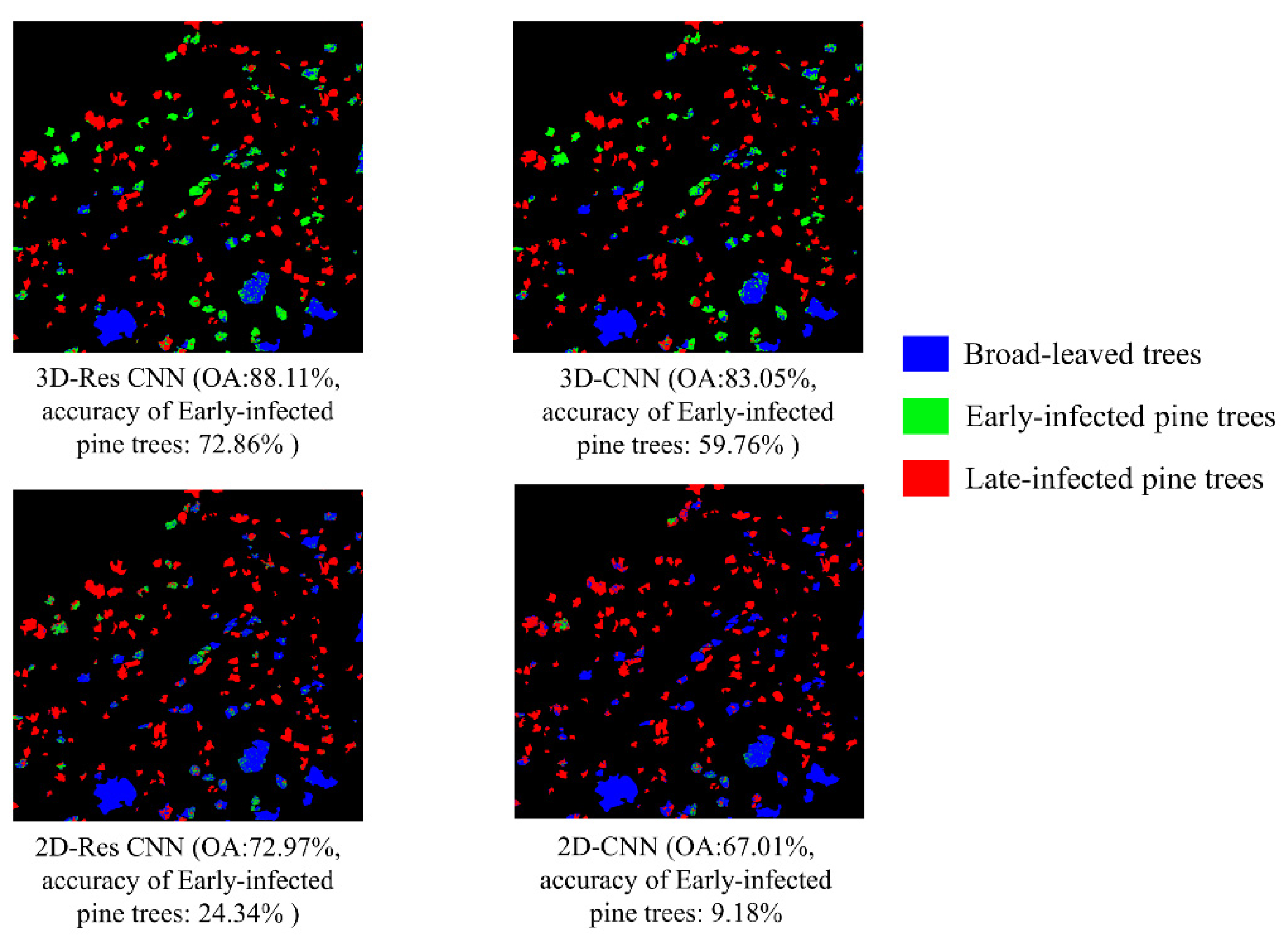
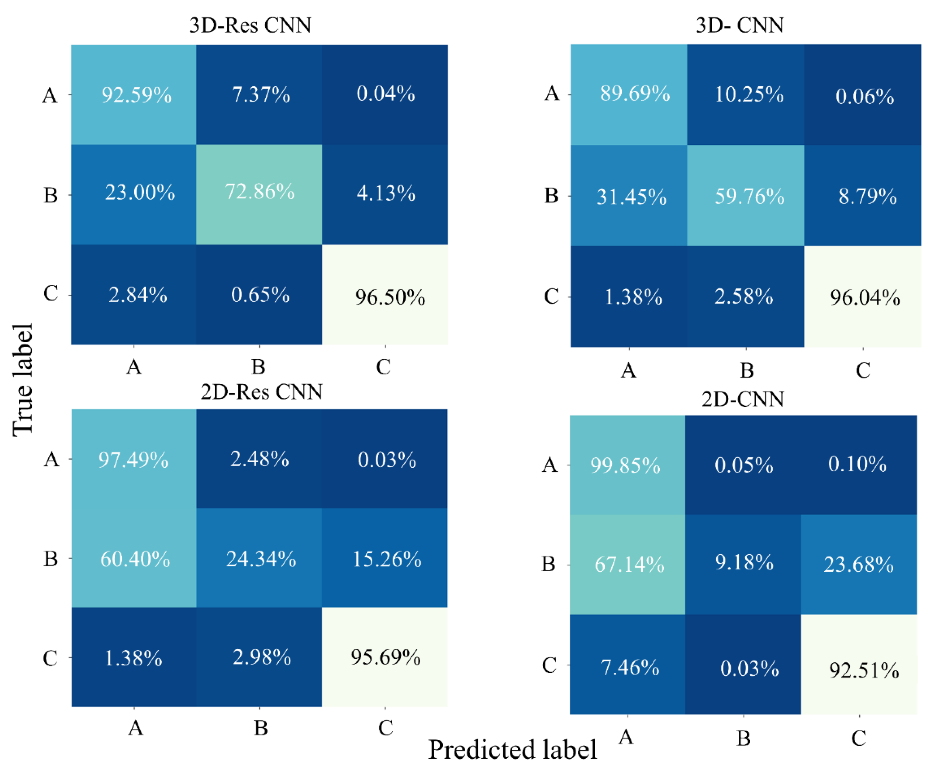
| Model | 2D-CNN | 2D-Res CNN | 3D-CNN | 3D-Res CNN |
|---|---|---|---|---|
| OA (%) | 67.01 | 72.97 | 83.05 | 88.11 |
| AA (%) | 67.18 | 72.51 | 81.83 | 87.32 |
| Kappa × 100 | 49.44 | 58.25 | 73.37 | 81.29 |
| Early infected pine trees (PA%) | 9.18 | 24.34 | 59.76 | 72.86 |
| Late infected pine trees (PA%) | 92.51 | 95.69 | 96.04 | 96.51 |
| Broad-leaved trees (PA%) | 99.85 | 97.49 | 89.69 | 92.58 |
| Trainable parameters | 47,843 | 47,843 | 117,219 | 117,219 |
| Trainable time (minute) | 34 min | 35 min | 100 min | 115 min |
| Prediction time (second) | 14.3 s | 14.8 s | 20.1 s | 20.9 s |
Publisher’s Note: MDPI stays neutral with regard to jurisdictional claims in published maps and institutional affiliations. |
© 2021 by the authors. Licensee MDPI, Basel, Switzerland. This article is an open access article distributed under the terms and conditions of the Creative Commons Attribution (CC BY) license (https://creativecommons.org/licenses/by/4.0/).
Share and Cite
Yu, R.; Luo, Y.; Li, H.; Yang, L.; Huang, H.; Yu, L.; Ren, L. Three-Dimensional Convolutional Neural Network Model for Early Detection of Pine Wilt Disease Using UAV-Based Hyperspectral Images. Remote Sens. 2021, 13, 4065. https://doi.org/10.3390/rs13204065
Yu R, Luo Y, Li H, Yang L, Huang H, Yu L, Ren L. Three-Dimensional Convolutional Neural Network Model for Early Detection of Pine Wilt Disease Using UAV-Based Hyperspectral Images. Remote Sensing. 2021; 13(20):4065. https://doi.org/10.3390/rs13204065
Chicago/Turabian StyleYu, Run, Youqing Luo, Haonan Li, Liyuan Yang, Huaguo Huang, Linfeng Yu, and Lili Ren. 2021. "Three-Dimensional Convolutional Neural Network Model for Early Detection of Pine Wilt Disease Using UAV-Based Hyperspectral Images" Remote Sensing 13, no. 20: 4065. https://doi.org/10.3390/rs13204065
APA StyleYu, R., Luo, Y., Li, H., Yang, L., Huang, H., Yu, L., & Ren, L. (2021). Three-Dimensional Convolutional Neural Network Model for Early Detection of Pine Wilt Disease Using UAV-Based Hyperspectral Images. Remote Sensing, 13(20), 4065. https://doi.org/10.3390/rs13204065