Article

Dielectric Properties of Lunar Materials at the Chang’e-4 Landing Site

1
School of Science, Jiangxi University of Science and Technology, Ganzhou 341000, China
2
State Key Laboratory of Lunar and Planetary Sciences, Macau University of Science and Technology, Macau 999078, China
*
Author to whom correspondence should be addressed.
Remote Sens. 2021, 13(20), 4056; https://doi.org/10.3390/rs13204056
Submission received: 27 August 2021 / Revised: 27 September 2021 / Accepted: 3 October 2021 / Published: 11 October 2021
(This article belongs to the Special Issue Planetary Remote Sensing: Chang’E-4/5 and Mars Applications)

Abstract

:
On January 3rd 2019, the Chang’e-4 mission successfully landed in the Von Kármán Crater inside the South Pole-Aitken (SPA) basin and achieved the first soft landing on the farside of the Moon. Lunar penetrating radar (LPR) equipped on the rover measured the shallow subsurface structure along the motion path for more than 700 m. LPR data could be used to obtain the dielectric properties of the materials beneath the exploration area, providing important clues as to the composition and source of the materials. Although the properties of the upper fine-grained regolith have been studied using various methods, the underlying coarse-grained materials still lack investigation. Therefore, this paper intends to estimate the loss tangent of the coarse-grained materials at depth ranges of ~12 and ~28 m. Stochastic media models with different rock distributions for the LPR finite-difference time-domain (FDTD) simulation are built to evaluate the feasibility of the estimation method. Our results show that the average loss tangent value of coarse-grained materials is 0.0104 ± 0.0027 , and the abundance of F e O T + Ti O 2   is   20.08   wt . % , which is much higher than the overlying fine-grained regolith, indicating different sources.

Graphical Abstract

1. Introduction

In January 2019, the Chang’e-4 lander successfully landed in the Von Kármán Crater on the lunar farside, becoming the first probe to land on the farside of the moon. The Yutu-2 rover is equipped with instruments including a multi-antenna, two channels (channel one and two) lunar penetrating radar (LPR) system. The central frequency of channel one is 60 MHz, which is utilized to detect the relatively deep part of the subsurface structure, specifically the basalt layered structure, basalt thickness, etc. The central frequency of channel two is 500 MHz, which is used to detect the shallow subsurface of the lunar regolith, including the thickness of the lunar regolith and the depth of the basalt layer and the physical parameters of the lunar regolith, such as the electrical constant, loss tangent and density [1,2].
Up to now, most lunar missions have been flyby or orbital explorations, and the more than 20 landing sites are all on the nearside of the Moon. Therefore, the successful implementation of the Chang’e-4 exploration mission provides an unprecedented opportunity to observe the subsurface structure of the lunar farside [3].
The landing site of the Chang’e-4 is located at 177.588° E, 45.457° S in the Von Kármán Crater, marked by a red triangle in Figure 1 [4,5]. The Von Kármán Crater is inside the South Pole-Aitken (SPA) basin, the largest and oldest impact crater on the Moon. According to the spectrum results and impact numerical simulation, it is generally believed that the Aitken Basin at the Lunar South Pole sputters the lower lunar crust and even the upper lunar mantle material on the lunar surface, so SPA Basin has important research value to understand the lunar interior and history [6]. The Von Kármán Crater has experienced multiple impact ejecta filling events and multiple stages of lava flow filling [7,8,9]. This complex geological history has brought uncertainty to the interpretation of the Chang’e-4 LPR data. Huang et al. (2018) utilized the Lunar Reconnaissance Orbiter Camera (LROC) Wide-Angle Camera (WAC) data to obtain the global normalized reflectance image, and found that crater rays and secondary crater chains around the Chang’e-4 landing site pointed to the Finsen Crater [7]. In situ spectral data collected by the Yutu-2 rover showed that the characteristics of surface materials around the motion path are similar to those of Finsen’s ejecta, which were analyzed with the Moon Mineralogy Mapper spectral data. This may indicate that the deposits in these two locations share the same source [10,11]. Furthermore, Lai et al. (2020) used the impact crater ejecta empirical model to estimate the ejecta thickness of the Finsen Crater in the Chang’e-4 landing site to be 7.9 meters, close to the thickness of the lunar regolith based on the radar observation [12]. In summary, recent research showed that there is a 12 m-thick fine regolith layer under the Yutu-2 rover’s motion path, and most of surficial materials came from the Finsen Crater [13,14,15,16,17].
Chang’e-4 LPR observed an important feature of the subsurface structure of the landing site—at a depth of about 12 m, there is a clear boundary between fine and coarse materials (Section 2.1). The fine materials are interpreted as fine-grained regolith, mainly formed by the deposits from Finsen [13]. The coarse materials are recognized as impact ejecta resulting from multiple impact events [16].
The composition and the properties of the fine-grained regolith were analyzed carefully using the in situ LPR data and spectral data. Lai et al. (2019), Li et al. (2020) and Dong et al. (2020) utilized the hyperbola fitting method to estimate the permittivity and density of the subsurface fine regolith [13,14,18]. The permittivity value of the fine regolith layer was estimated to be ~4. Lai et al. (2019) used signal loss to calculate the loss tangent of the fine-grained regolith layer, which was about 0.0039 [13]. Li et al. (2020) determined the average loss tangent of the fine-grained material under the Chang’e-4 landing site to be   ( 5 ± 2 ) × 10 3 , based on the shifting of the centroid frequency with the depth. Since the loss tangent value is smaller than the normal value of the mare basalt, an intact, dense lava flow layer is excluded from possibility [14]. Dong et al. (2021) utilized the surface, subsurface reflections and the incident pulse amplitude to infer the permittivity and density of the fine-grained regolith layer [19]. They also obtained the surface permittivity of the Chang’e-4 landing site for the first time. Dong et al. utilized the empirical model developed with measurements of lunar samples to obtain the loss tangent of the fine-grained regolith layer materials, which was ( 4.4 ± 0.5 ) × 10 3 [19]. Based on the 3D velocity spectrum method, Dong et al. (2020) calculated the properties of the subsurface materials, including velocity, relative permittivity, etc. [20]. Li and Zhang used the migration method and separated the diffractions from reflections to estimate the permittivity and density up to 50 meters [21]. Although the properties of fine materials under the Chang’e-4 landing site have been inversed by various methods, there is still a lack of studies on the properties and source of the coarse materials, such as the loss tangent parameter. The loss tangent and the permittivity of the materials are the most important indicators for the composition of materials on the Moon, which can be further used to speculate on the source of the materials and acquire a better understanding of the geological structure and history around the Chang’e-4 landing site. In this paper, we utilize the Chang’e-4 LPR data of channel two to estimate the loss tangent of the coarse and sub-surface materials and indicate F e O T + Ti O 2 content.
This paper is organized as follows. Section 2 introduces the LPR data processing method, the estimation method of the loss tangent and the stochastic media models. In Section 3, the results of three simulation models are given to verify the feasibility of the loss tangent estimation method, which is applied to the LPR data. A detailed discussion on the results of the three simulation models and LPR data, including the estimated loss tangent and the total F e O and T i O 2 contents of coarse materials inferred using empirical formulas, is given in Section 4. Section 5 contains the conclusion.

2. Materials and Methods
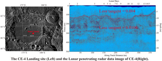
2.1. LPR Data

Channel two of LPR has one transmitting and two receiving antennas, which are deployed on the bottom of the Yutu-2 rover, named as 2A and 2B, respectively. In this study, we only analyzed LPR 2B data. The bandwidth of LPR channel 2B is 450 MHz, which indicates that the resolution is 0.3 m in a vacuum [22]. The Yutu-2 rover has been working on the Moon for more than two years, and the LPR has detected a more than 700 m long subsurface structures along its motion path. The first 15 days of LPR data were utilized in this work (Figure 2). The Data File IDs were listed in Table S2.
Data preprocessing is necessary before interpreting radar data. Based on the characteristics of the Chang’e-4 LPR data, a set of preprocessing methods is proposed [13]. In this paper, the data processing scheme is modified to retain the original amplitude information.
  • Data reading: 2B processing-level data are utilized in the paper, which are generated with raw data after integration, conversion from unsigned integers to signed integers, normalization, removing direct current offset, and adding geometric coordinates.
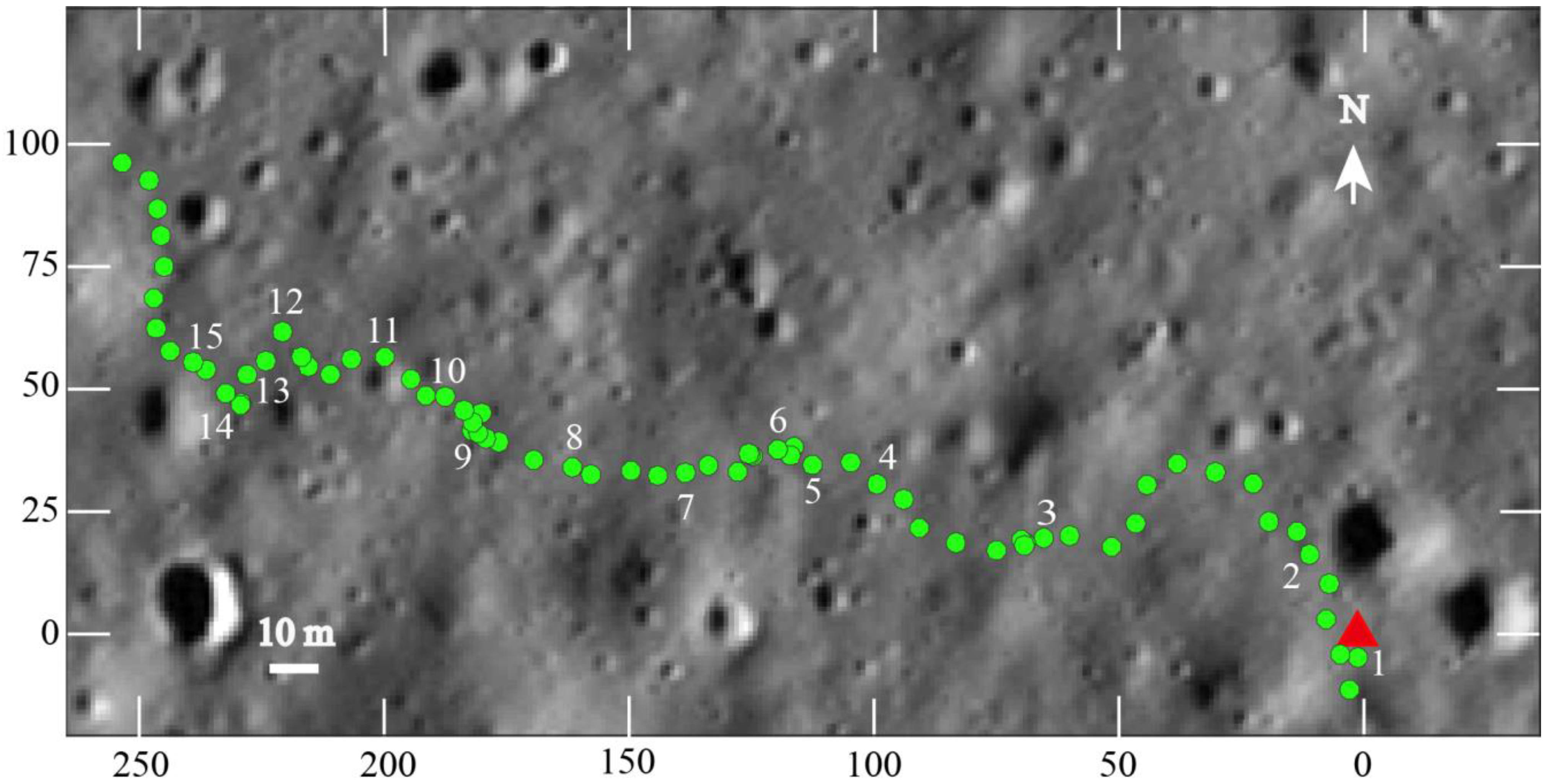
  • Redundant data removal: when LPR is operating, the Yutu-2 rover may stop to perform the operations of other instruments, which generated duplicate data. So, data collected during static sampling should be removed.
  • Data file stitching: the files of different lunar days are stored separately. In this step, these data need to be stitched together.
  • Adjust the time delay: the receiving antenna is turned on 28.203 ns earlier than the transmitting antenna, so the initial 28.203 ns of all the data traces were removed.
  • Background removal: subtracting the average value from the LPR data to reduce the ‘ringing’ effects and periodic noises caused by the antenna–ground coupling.
  • Band-pass filter: the finite impulse response (FIR) filter is used to reduce noise. Its cut-off frequencies are set as 150, 250, 750, and 850 MHz.

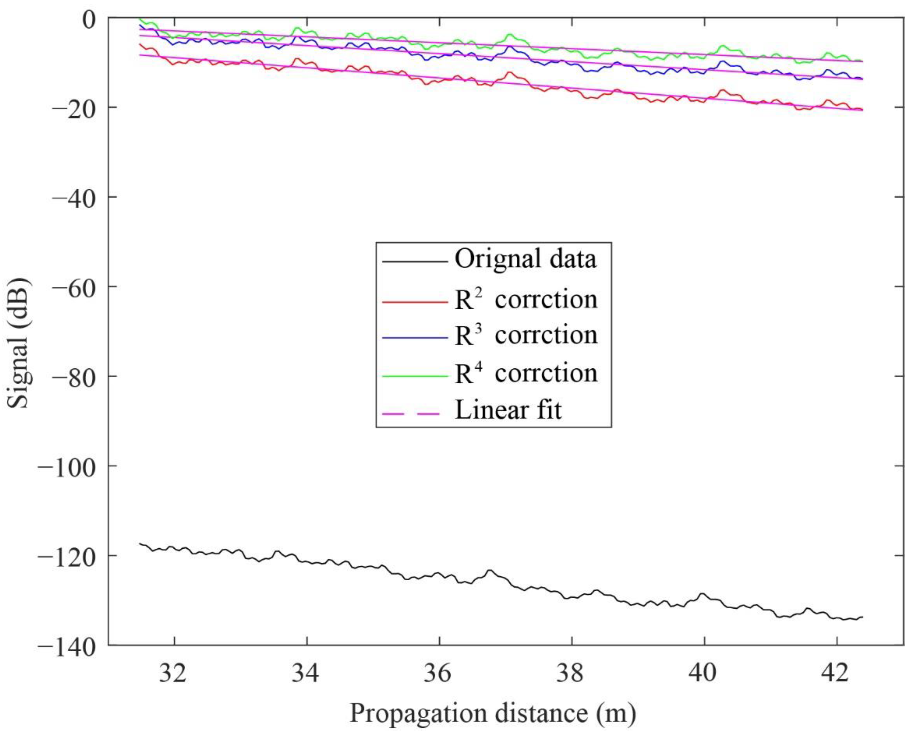
2.2. Loss Tangent Estimation Method

Grimm et al. proposed a method of measuring attenuation using ground penetrating radar [23]. The radar range equation, given in Skolnik [24], is:
P r P t = G 2 λ 2 ξ ( 4 π ) 3 R 4 e 4 α R
where   P r is the received power, P t is the transmitted power, G is the system gain, λ is the wavelength in the medium, ξ is the backscatter cross section, e 4 α R is the attenuation in the medium, and α   is the spatial attenuation coefficient. Later, α can also be expressed as η ( α in dB) in unit dB / m , η = 20 log 10 ( e α ) = 8.686 α .
In general, α can be expressed as the following formula [25]:
α = ω μ ε 2 ( 1 + tan 2 δ 1 )  
where ω is the angular frequency, μ is the magnetic permeability, ε is the dielectric permittivity, and tan δ is the loss tangent. For a lunar sample, tan δ 1 , and μ is assumed to be the free space magnetic permeability. Then,
η = 9.1 × 10 8 ε f tan δ
where ε is the real part of the relative permittivity.
Formula (1) indicates that the attenuation loss can be divided into two parts—the scattering loss and the intrinsic (or absorption) loss. If the scattering loss can be effectively compensated for, then the absorption loss can be estimated.
For different reflected targets, the ratio between the received power and the transmitted power is proportional to the reciprocal power of the propagation distance:
P R / P t 1 / R n
In this case, three different models of reflected targets are considered: n = 2 for a planar and smooth reflected target; n = 3 for the Fresnel zone case; and n = 4 for discrete scatters. After compensating for the scatter signals, the attenuation η can be estimated by least squares fitting of the two-way distance versus the ratio of the transmitted power to received power in unit dB / m . After obtaining the attenuation η , tan δ can be estimated by Formula (3).

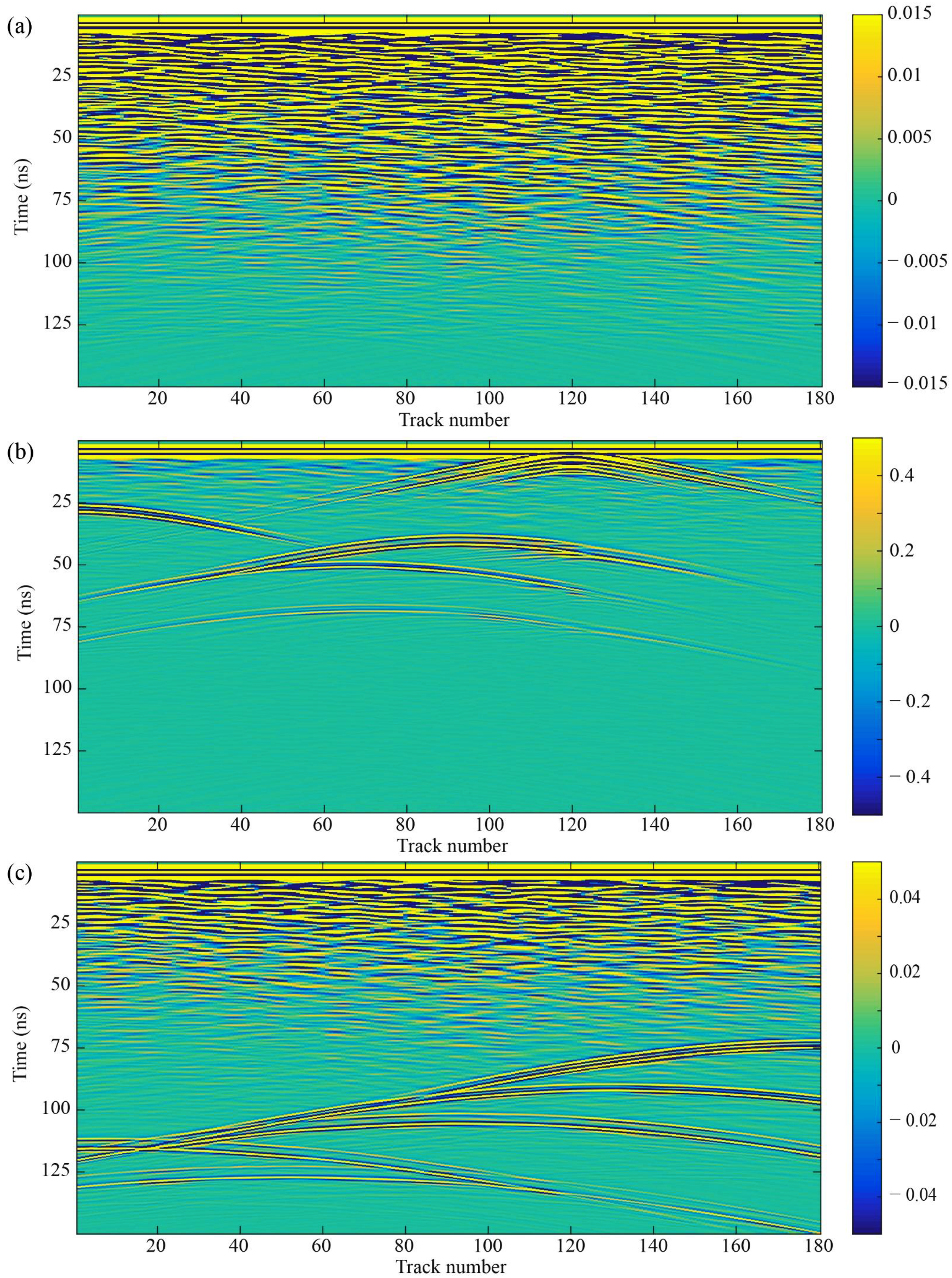
2.3. Simulation Model

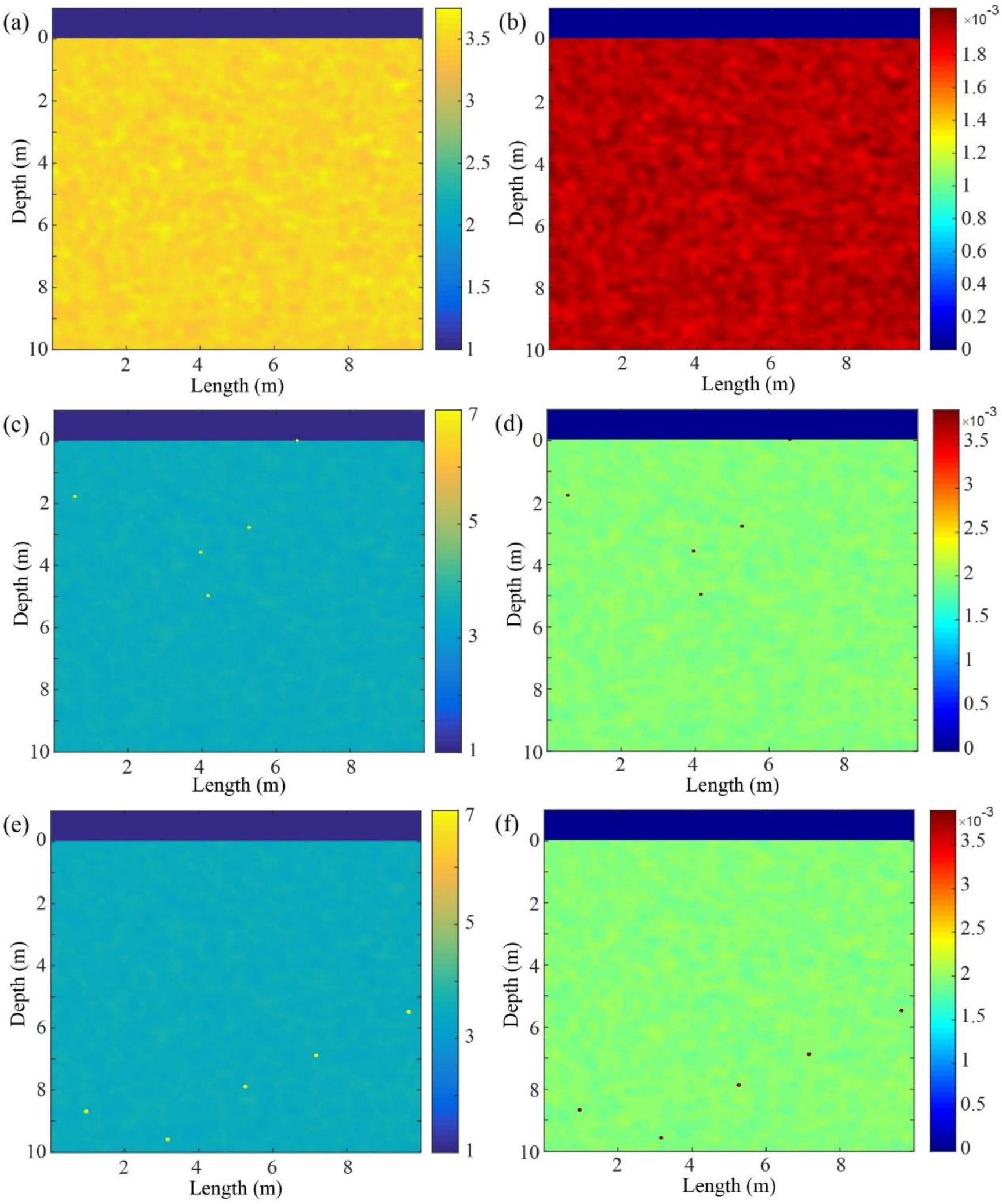
2.3.1. Stochastic Media Model

In order to verify the feasibility of the loss tangent estimation method, a simulation model was utilized. Previous studies have shown that the internal structure of the lunar regolith is close to the stochastic media model [26]. Hence, the stochastic media model with an ellipsoidal autocorrelation function was used in this study to simulate the lunar regolith structure [27]. The method is described as follows:
1. A two-dimensional stochastic equivalent medium model is established by using ellipsoidal autocorrelation function:
f ( x , y ) = e x p [ ( x 2 a 2 + y 2 b 2 ) ] 1 1 + r
where r is the fuzzy factor of the stochastic media model, and a and b represent the autocorrelation length in the X and Y directions, respectively.
2. The f (x, y) is transformed into the wavenumber domain (F ( k x , k y ) ) by the two-dimensional Fourier transform equation, and then the power spectrum function R ( k x , k y )   is calculated.
R ( k ) = F ( k x , k y ) 2
3. Generate the independent and uniform random numbers ϕ ( k x , k y ) in the range of [ 0 , 2 π ) .
4. By adding the random number ϕ ( k x , k y )   into Formula (7), a new energy spectral density function is obtained:
F ( k x , k y ) = R ( k ) e x p [ + i ϕ ( k x , k y ) ]
5. The inversed two-dimensional Fourier transform is performed to transform F ( k x , k y ) from the wavenumber domain to the spatial domain to obtain a new f ( x , y ) .

2.3.2. Simulation Model

In order to model different scenarios of lunar regolith structure, three stochastic media models were used. Model One is shown in Figure 3a. In the models (e.g., Figure 3a,b), the material of the first layer is free space. Model Two and Model Three have the same layered structure, but with different abundances and distribution of rocks. Five rocks are placed in the upper part of Model Two, while in Model Three, they are in the lower part. The autocorrelation lengths in the X and Y directions are both 2. The fuzzy factor r is 0 in this model. The model is 10 m in length, and 11 m in depth, and the spatial steps in the X (length) and Y (depth) direction are both 0.005 m. The time window is 150 ns, the time step is 0.0118 ns. The moving steps of both transmitter and receiver antenna are 0.05 m. The average permittivity of background material is 3.5, which is consistent with the result of Lai et al. [13] and Wang et al. [15]. The relative loss tangent is set as 0.02, which indicates the average conductivity of the model is about 2 × 10 3 (e.g., Figure 3b). The transmitter antenna and receiver antenna are 0.3 m higher than the zero depth. The range between the transmitter antenna and the receiver antenna is 0.32 m, the same as the settings of the Chang’e 4 LPR.

3. Results

3.1. Synthetic Data Results
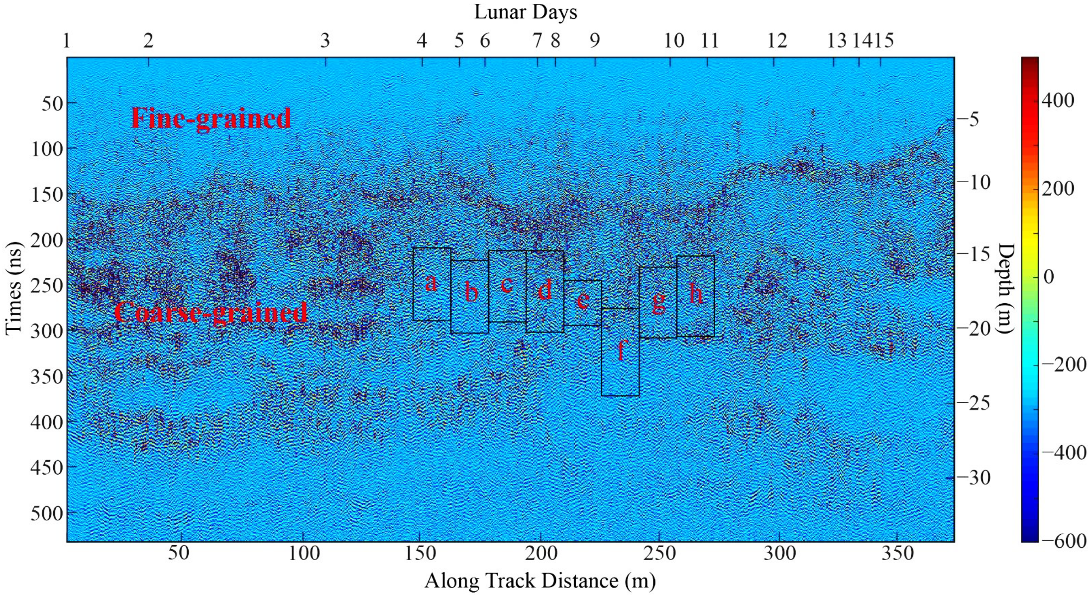
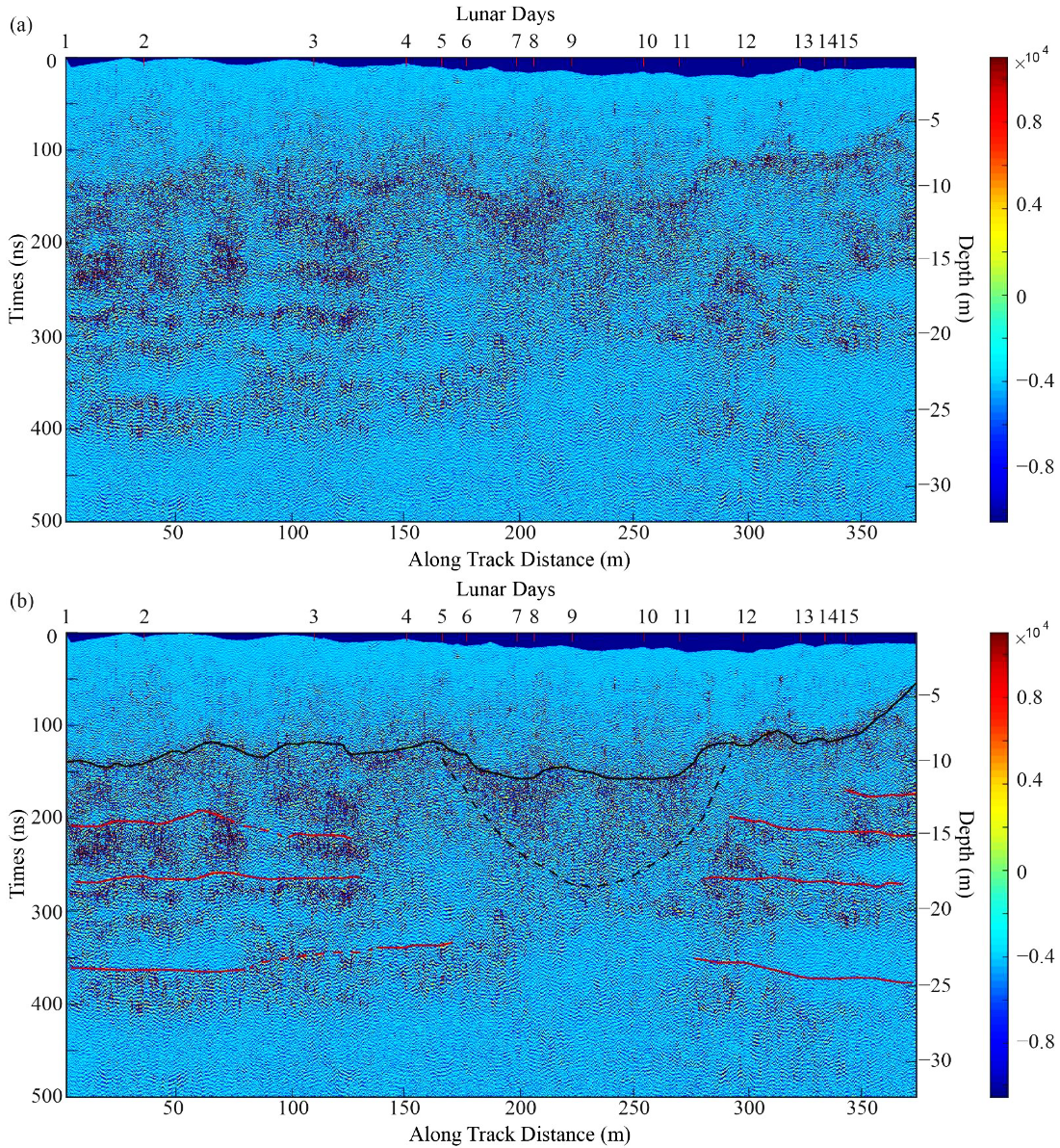
The finite-difference time-domain (FDTD) simulation method is utilized to verify the correctness of the loss tangent estimation method, which is mentioned in Section 2.2. gprMax software, an open source software package for numerical modeling of ground penetrating radar (GPR), is used for simulation [28]. It is foreseeable that the reflection signal of the buried rock and the multiple scattering signals among the rocks will affect the results of the loss tangent estimation, so three models are used in this experiment to evaluate the influence of rocks. The base stochastic media model is the same for these three models, except for locations of the rocks. Figure 4 shows the comparisons between the simulation results of these three models.
The method mentioned in Section 2.2 is utilized to estimate the loss tangent of the simulation model. In order to reduce the influence of noises, the mean square of each radar trace is calculated before estimating the loss tangent. Figure 5 shows the estimated attenuation result.
In Figure 5, the red, blue and green lines represent the synthetic data after R2, R3, and R4 backscatter/spreading correction, respectively. The dashed purple line indicates the least linear fitting results. The slope of the dashed purple line is equal to the attenuation η . Then, Formula (3) is used to calculate loss tangent parameters. Table 1 shows the attenuation’s estimated result.
The average loss tangent of Model One is 0.0229 ± 0.0084 , which is consistent with the simulation model (0.02). The average loss tangents of Model Two and Model Three are 0.0273 ± 0.0061 and 0.0156 ± 0.0134 , respectively. Thus, the presence of rocks introduces some errors to the results, but within a tolerable range. The error of results of Model Two and Model Three is 36.5% and 22%, respectively. The distribution of rocks also affects the inferred loss tangent. In this example, the rocks at the bottom result in fewer errors of the estimated result than that of rocks in the upper part. Next, the algorithm will be used in the Chang’e-4 LPR data.

3.2. LPR Results

The loss tangent estimation method introduced in Section 2.2 is used to calculate the loss tangent of the coarse material. In order to mitigate the influence of the rocks, we only select the depth range of relatively uniform materials (the sampling time exceeds 150ns for the 6th to the 12th lunar days in Figure 6 have been selected. After averaging the energy of adjacent 437 tracks of LPR data, which is obtained after data preprocessing described in Section 2.1, the original root mean square data are obtained (black line in Figure 7). Then, the spreading and backscatter correction factor (R2, R3, R4) are utilized to compensate for the spreading and backscatter loss. Then, the least squares fitting method is used to fit the data after exponential function compensation (dashed purple lines in Figure 7). The estimated results of signal attenuation of LPR data are shown in Figure 7. The corresponding loss tangent results are given in Table 2.

4. Discussion

4.1. Loss Tangent of the Simulation Model

Figure 5 and Table 1 show estimated results of the loss tangent of the simulation models. For the simulation model, the R3 correction result, which indicates that reflections come from a Fresnel-zone sized area, is plausible. The loss tangent of Model One after R3 correction is 0.0229 , compared to the parameter ~0.02 used in the stochastic media model, and the error is less than 15%. Taking into account the result after over-compensation (R4 correction) and under-compensation (R2 correction), the real value is within the range of estimation values ( 0.0229 ± 0.0084 ). Therefore, the simulation results show that the estimation method can effectively obtain the loss tangent when little rock is present.
Model Two includes five stones in the upper part of layer two. It is expected that the reflection signal from the rocks and the scattering signal among the rocks will affect the radar signals. The locations of rocks are known in the simulation model. The deepest rock is placed at the propagation distance of about 10 m, so we selected the echo signal with a propagation distance between 14 and 19 meters to calculate the energy attenuation curve. The average loss tangent of Model Two is 0.0273 ± 0.0061 , which is higher than the actual setting. Judging from the results, rocks cause scattering of the EM wave and result in a slightly larger loss tangent than the simulation parameter, as the interference of rocks increases the signal attentions. Therefore, avoiding rocks in the calculation area could improve the accuracy of the loss tangent. However, if rocks are ubiquitous, the result can also be considered as the upper limit of the loss tangent.
Model Three has five stones distributed on the bottom. The shallowest rock is about ~10 m in propagation distance, so we selected the echo signal with a propagation distance between 6 and 8.5 m to calculate the energy attenuation curve. The average loss tangent of Model Three is 0.0231 ± 0.0144 , which is consistent with the real setting and better than the case in which rocks are above the study region (Model Two). Hence, the result of the loss tangent can be improved by selecting the area of calculation appropriately. It is worth noting that although the results of Model One and Model Two are similar, the confidences of these two models (0.0084 vs. 0.0144) are different due to the different horizontal length of the calculation area. Increasing the calculation area can reduce the confidence interval. In addition, by comparing Model One and Model Three, it can be concluded that a longer calculation interval in depth could reduce the error bar.
In actual situations, if the selected area contains rocks in the lower part, the tail of the energy attenuation curve may go up, resulting in the estimated loss tangent being smaller than the actual situation. For example, in Model Three, the calculation area is expanded to 9.5 m, so the rocks are included, then the average loss tangent is changed to 0.0156 ± 0.0133 . In this case, it can be considered that the calculated loss tangent is the lower limit of the actual situation.

4.2. Loss Tangent of the Coarse Material

Figure 6 shows the LPR data after processing with the steps proposed by Lai et al. [13]. The significant feature of the LPR image is that there is a continuous horizontal reflection around the depth of ~12 m. In order to calculate the loss tangent of coarse materials, a study area in the depth range of ~146 to ~273 m on the Yutu-2 rover’s motion path was selected in this study. LPR data were divided into a set of groups along the horizontal direction, with each group being 15 m long. The total number of groups is eight, which are named as group a, b, …, h, respectively (Figure 6). The attenuation of these eight groups was calculated separately, and the corresponding results are shown in Figure 7 and Table 2. Then, we utilized Formula (3) to estimate the loss tangent. From Figure 7 and Table 2, it can be seen that each data group used different depth ranges to calculate the loss tangent to reduce the noises caused by rocks. Table 2 shows that the estimated loss tangent of groups a, b, c, d, g and h are similar, the average value of which is 0.0105. The estimated loss tangent of group e is larger than the average result, while group f’s value is smaller.
The main reason for deviations in the estimation results is that there are several energy bumps (Figure 7e) at bottom (40–43m) of the group e, probably due to rock scattering, which causes the result of group e to be relatively small. The group e can be regarded as the situation that the tail of the energy attention curve is affected by the rock reflection signal, which is similar to the situation of Model three, and it can be considered as the lower limit of the loss tangent.
From Figure 7, the energy attenuation curve of group f changes relatively smoothly compared to other groups, and the error bar is smaller than those of other groups. However, the loss tangent of group f is larger than the average value, which may indicate that some rocks might be distributed above the selected area. Similar to the results of Model Two, scattering caused by rocks affects the estimation of loss tangent. In this situation, the upper limit of the loss of coarse materials can be obtained.
In groups a, b, c and d, the maximum value of the estimated loss tangent after R3 correction is 0.0112 and the minimum value is 0.0101. The difference between these two values is about 10%. To improve the confidence of the results, the sampled data on a longer motion path are used to calculate the energy attenuation curve and then estimate the loss tangent. In this study, we use the energy attenuation curve of adjacent 1700 tracks of LPR data to re-estimate the loss tangent, and obtain Figure 8.
The corresponding result of Figure 7 is calculated in Table 3.
From Figure 8, we can conclude that increasing the size of the calculation area can effectively improve the R-square value, and can fit the curve better to reduce the error bars. The average value of the loss tangent is 0.0104, which is consistent with the average value of the loss tangent of group a, b, c, d, g and h (0.0105).
Based on the previous analysis, it is concluded that the estimated average loss tangent of the coarse materials in the calculated area is 0.0104 ± 0.0027 . If empirical results of the simulation model are used, the upper limit of the loss tangent is 0.0120, and the lower limit is 0.087.

4.3. The Geological History of the Chang’e-4 Landing Site

In radargrams, there are continuous horizontal reflectors inside the coarse-grained materials [13,14,15,16,17]. Zhang et al. (2020) argued that there are 4-5 layers of impact ejecta blanket coverage between 12 and 40 meters under the motion path of the Yutu-2 rover [16]. Xu et al. (2021) found four impact craters (the thickness of the local materials and ejecta deposits are more than 1 meter) that can have a greater impact on the landing site through the model [29]. In order to better analyze the subsurface structure of the landing site, the migration method and topographic correction are applied to the radargram in Figure 2. Figure 9a shows the radar image after processing. There are some horizontal reflectors around ~210, ~270 and ~360 ns, which are marked by red lines in Figure 9b. These continuous interface reflections appear on both sides of the loss tangent estimated area (Figure 6 and Figure 9). The interruption of the continuity is because of a bowl-shaped area marked by the black dotted line in Figure 9b. Zhang et al. (2021) and Zhou et al. (2021) believed that this area is a buried impact crater, and the continuous reflective interfaces were destroyed by the subsequent impact event [30,31]. The materials under the impact crater were mixed and are relatively uniform, so the loss tangent estimation model can be applied. The estimated loss tangent is the loss tangent of the mixed multi-layered coarse materials.
Considering that the central frequency of the Yutu-2 high-frequency radar is 500 MHz, the empirical formula based on the data points only representing measurements at 450 MHz is utilized [32].
tan δ = 10 ( 0.038 × ( % T i O 2 + % F e O ) 2.746 )
Substitute the average loss obtained by the previous calculation (0.0104) into Formula (8), and then we can obtain the total F e O T and T i O 2 concentrations of the coarse materials at the CE-4 landing site as 20.08 wt.%. Additionally, with the upper and lower loss tangent bounds (0.0120 and 0.0087), the total F e O T + T i O 2 concentrations will be 21.7 and 18.0 wt.%, respectively. The F e O T + T i O 2 concentration of the surface fine materials around the Chang’e-4 landing site is lower than 15 wt.%, and the T i O 2 content of which is between 1 and 2 wt.% [9,33,34,35,36]. This value is below even the lowest boundary estimates based on Equation (8) of the coarse materials. This may indicate that the surface fine material has much lower F e O T content than that of the underlying coarse substance, and may share a different source. Qiao et al. (2019) proposed that dozens of craters (about 330 m–1.1 km in diameter) have relatively high F e O T in the crater interiors and ejecta blankets [36]. The high F e O T + Ti O 2 concentrations of the coarse materials may be caused by the iron-rich nature of the ejecta blankets.

5. Conclusions

In this study, we use signal attenuation to estimate the loss tangent value of the coarse material in lunar regolith beneath the motion path of the Chang’e-4 rover. Three stochastic media models are utilized to verify the estimation method. The simulation results demonstrate that the estimation is close to the real setting when the propagation medium is uniform with little scattering, and the error is about 15%. If, however, scattering targets are present in the study area, the results will be affected. For example, the result becomes larger when rocks appear above the calculation area. In this case, the estimated result can be considered as the upper limit of the loss tangent. When the rocks appear below the calculation area, the estimated result is smaller than the actual value. In addition, increasing the calculation area could improve the confidence of the estimation results.
The average loss tangent value of the coarse materials in the Chang’e-4 landing site is about 0.0104; considering the influence of the rocks, the upper limit of the loss tangent is 0.0120, and the lower limit is 0.087. Based on the empirical model of Apollo samples, the total F e O T and T i O 2 content of coarse-grained materials was estimated to be 20.08 wt.%, higher than that of the upper fine-grained materials, which indicates different origins of these two parts.

Supplementary Materials

The following are available online at https://www.mdpi.com/article/10.3390/rs13204056/s1, Table S1: IDs of LPR CH-2 data.

Author Contributions

Conceptualization, J.L., F.C. and Y.X.; formal analysis, J.L., F.C. and Y.X.; data curation, J.L. and F.C.; methodology, J.L., F.C. and L.Z.; validation, J.L., F.C. and L.Z.; writing—original draft preparation, J.L., F.C. and Y.X.; supervision, Y.X. and C.L.; funding acquisition, J.L., Y.X. and C.L. All authors have read and agreed to the published version of the manuscript.

Funding

Scientific data are provided by the China National Space Administration (CNSA). We are grateful for the support from the team members of the Ground Application and Research System (GRAS), who contributed to data receiving and preprocessing. This research was funded by the Science and Technology Development Fund (FDCT) of Macau (Grants 0042/2018/A2, 0089/2018/A3, 0079/2019/A2, and 0049/2020/A1), the Pre-research Project on Civil Aerospace Technologies of CNSA (D020101), The National Natural Science Foundation of China, grant number 12103020, 11875149; the Science and technology project of Jiangxi education department, grant number GJJ200821 and the Scientific Research Starting Foundation for scholars from Jiangxi University of Science and Technology, grant number jxxjbs18017, The Youth Jinggang Scholars Program in Jiangxi Province, and The Program of Qingjiang Excellent Yong Talents, Jiangxi University of Science and Technology.

Institutional Review Board Statement

Not applicable.

Informed Consent Statement

Not applicable.

Data Availability Statement

CE-4 LPR data are available at Data Publishing and Information Service System of China’s Lunar Exploration Program (http://moon.bao.ac.cn). All the LPR data IDs are listed in Supplementary Table S1. Data sources of Figure 1 and Figure 2 are given in the captions.

Acknowledgments

Scientific data are provided by the China National Space Administration (CNSA). We are grateful for the support from the team members of the Ground Application and Research System (GRAS), who contributed to data receiving and preprocessing.

Conflicts of Interest

The authors declare no conflict of interest.

References

  1. Fang, G.-Y.; Zhou, B.; Ji, Y.-C.; Zhang, Q.-Y.; Shen, S.-X.; Li, Y.-X.; Guan, H.-F.; Tang, C.-J.; Gao, Y.-Z.; Lu, W.; et al. Lunar Penetrating Radar onboard the Chang’e-3 mission. Res. Astron. Astrophys. 2014, 14, 1607–1622. [Google Scholar] [CrossRef]
  2. Jia, Y.Z.; Zou, Y.L.; Ping, J.S.; Xue, C.B.; Yan, J.; Ning, Y.M. The scientific objectives and payloads of Chang’E−4 mission. Planet. Space Sci. 2018, 162, 207–215. [Google Scholar] [CrossRef]
  3. Wu, W.R.; Liu, J.Z.; Tang, Y.H.; Yu, D.Y.; Yu, G.B.; Zhang, Z. China Lunar Exploration Program. J. Deep Space Explor. 2019, 6, 405–416. [Google Scholar] [CrossRef]
  4. Robinson, M.S.; Brylow, S.M.; Tschimmel, M.; Humm, D.; Lawrence, S.J.; Thomas, P.C.; Denevi, B.; Bowman-Cisneros, E.; Zerr, J.; Ravine, M.A.; et al. Lunar Reconnaissance Orbiter Camera (LROC) Instrument Overview. Space Sci. Rev. 2010, 150, 81–124. [Google Scholar] [CrossRef]
  5. Barker, M.K.; Mazarico, E.; Neumann, G.A.; Zuber, M.T.; Haruyama, J.; Smith, D.E. A new lunar digital elevation model from the Lunar Orbiter Laser Altimeter and SELENE Terrain Camera. Icarus 2016, 273, 346–355. [Google Scholar] [CrossRef] [Green Version]
  6. Li, C.; Liu, D.; Liu, B.; Ren, X.; Liu, J.; He, Z.; Zuo, W.; Zeng, X.; Xu, R.; Tan, X.; et al. Chang’E-4 initial spectroscopic identification of lunar far-side mantle-derived materials. Nat. Cell Biol. 2019, 569, 378–382. [Google Scholar] [CrossRef]
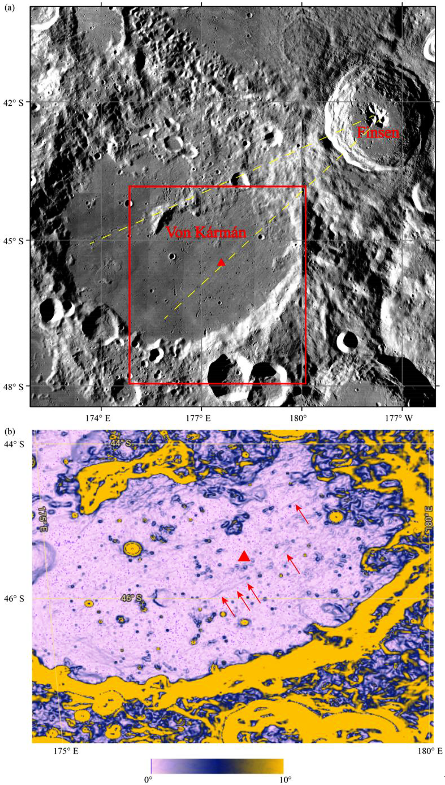
  7. Huang, J.; Xiao, Z.Y.; Flahaut, J.; Martinot, M.; Head, J.; Xiao, X.; Xie, M.G.; Xiao, L. Geological characteristics of Von Kármán crater, northwestern south pole-Aitken Basin: Chang’E-4 landing site region. J. Geophys. Res. Planet. 2018, 123, 1684–1700. [Google Scholar] [CrossRef] [Green Version]
  8. Pasckert, J.H.; Hiesinger, H.; van der Bogert, C.H. Lunar farside volcanism in and around the South Pole–Aitken basin. Icarus 2018, 299, 538–562. [Google Scholar] [CrossRef]
  9. Ling, Z.C.; Qiao, L.; Liu, C.Q.; Cao, H.J.; Bi, X.Y.; Lu, X.J.; Zhang, J.; Fu, X.H.; Li, B.; Liu, J. Composition, mineralogy and chronology of mare basalts and non-mare materials in Von Kármán crater: Landing site of the Chang’E−4 mission. Planet. Space Sci. 2019, 179, 104741. [Google Scholar] [CrossRef]
  10. Gou, S.; Yue, Z.; Di, K.; Bugiolacchi, R.; Wan, W.; Yang, M.; Ye, L. Geologically Old but Freshly Exposed Rock Fragments En-countered by Yutu-2 Rover. J. Geophys. Res. Planet. 2021, 126, e2020JE006565. [Google Scholar] [CrossRef]
  11. Lin, H.; He, Z.; Yang, W.; Lin, Y.; Xu, R.; Zhang, C.; Zhu, M.-H.; Chang, R.; Zhang, J.; Li, C.; et al. Olivine-norite rock detected by the lunar rover Yutu-2 likely crystallized from the SPA-impact melt pool. Natl. Sci. Rev. 2020, 7, 913–920. [Google Scholar] [CrossRef] [Green Version]
  12. Lai, J.; Xu, Y.; Bugiolacchi, R.; Meng, X.; Xiao, L.; Xie, M.; Liu, B.; Di, K.; Zhang, X.; Zhou, B.; et al. First look by the Yutu-2 rover at the deep subsurface structure at the lunar farside. Nat. Commun. 2020, 11, 1–9. [Google Scholar] [CrossRef] [PubMed]
  13. Lai, J.; Xu, Y.; Zhang, X.; Xiao, L.; Yan, Q.; Meng, X.; Zhou, B.; Dong, Z.; Zhao, D. Comparison of Dielectric Properties and Structure of Lunar Regolith at Chang’e-3 and Chang’e-4 Landing Sites Revealed by Ground-Penetrating Radar. Geophys. Res. Lett. 2019, 46, 12783–12793. [Google Scholar] [CrossRef]
  14. Li, C.; Su, Y.; Pettinelli, E.; Xing, S.; Ding, C.; Liu, J.; Ren, X.; Lauro, S.E.; Soldovieri, F.; Zeng, X.; et al. The Moon’s farside shallow subsurface structure unveiled by Chang’E-4 Lunar Penetrating Radar. Sci. Adv. 2020, 6, eaay6898. [Google Scholar] [CrossRef] [PubMed] [Green Version]
  15. Wang, R.; Su, Y.; Ding, C.; Dai, S.; Liu, C.; Zhang, Z.; Hong, T.; Zhang, Q.; Li, C. A Novel Approach for Permittivity Estimation of Lunar Regolith Using the Lunar Penetrating Radar Onboard Chang’E-4 Rover. Remote. Sens. 2021, 13, 3679. [Google Scholar] [CrossRef]
  16. Zhang, L.; Li, J.; Zeng, Z.; Xu, Y.; Liu, C.; Chen, S. Stratigraphy of the Von Kármán Crater Based on Chang’E-4 Lunar Pene-trating Radar Data. Geophys. Res. Lett. 2020, 47, e2020GL088680. [Google Scholar]
  17. Zhang, J.; Zhou, B.; Lin, Y.; Zhu, M.H.; Song, H.; Dong, Z.; Ouyang, Z. Lunar regolith and substructure at Chang’E-4 landing site in South Pole–Aitken basin. Nat. Astron. 2021, 5, 25–30. [Google Scholar] [CrossRef]
  18. Dong, Z.; Fang, G.; Zhao, D.; Zhou, B.; Gao, Y.; Ji, Y. Dielectric Properties of Lunar Subsurface Materials. Geophys. Res. Lett. 2020, 47, e2020GL089264. [Google Scholar] [CrossRef]
  19. Dong, Z.; Fang, G.; Zhou, B.; Zhao, D.; Gao, Y.; Ji, Y. Properties of Lunar Regolith on the Moon’s Farside unveiled by Chang’E-4 Lunar Penetrating Radar. J. Geophys. Res. Planet. 2021, 126, e2020JE006564. [Google Scholar] [CrossRef]
  20. Dong, Z.; Feng, X.; Zhou, H.; Liu, C.; Zeng, Z.; Li, J.; Liang, W. Properties Analysis of Lunar Regolith at Chang’E-4 Landing Site Based on 3D Velocity Spectrum of Lunar Penetrating Radar. Remote Sens. 2020, 12, 629. [Google Scholar] [CrossRef] [Green Version]
  21. Li, C.; Zhang, J. Velocity Analysis Using Separated Diffractions for Lunar Penetrating Radar Obtained by Yutu-2 Rover. Remote Sens. 2021, 13, 1387. [Google Scholar] [CrossRef]
  22. Su, Y.; Fang, G.-Y.; Feng, J.-Q.; Xing, S.-G.; Ji, Y.-C.; Zhou, B.; Gao, Y.-Z.; Li, H.; Dai, S.; Xiao, Y.; et al. Data processing and initial results of Chang’e-3 lunar penetrating radar. Res. Astron. Astrophys. 2014, 14, 1623–1632. [Google Scholar] [CrossRef]
  23. Grimm, R.E.; Heggy, E.; Clifford, S.; Dinwiddie, C.; McGinnis, R.; Farrell, D. Absorption and scattering in ground-penetrating radar: Analysis of the Bishop Tuff. J. Geophys. Res. Space Phys. 2006, 111. [Google Scholar] [CrossRef] [Green Version]
  24. O’Donnell, R.M. Introduction to Radar Systems; MIT OpenCourseWare, Primavera; Massachusetts Institute of Technology: Cambridge, MA, USA, 2007. [Google Scholar]
  25. Ward, S.H.; Hohmann, G.W. Electromagnetic Theory for Geophysical Applications. In Electromagnetic Methods in Applied Geophysics; Society of Exploration Geophysicists: Beijing, China, 1988; pp. 130–311. [Google Scholar]
  26. Zhang, X.; Lv, W.; Zhang, L.; Zhang, J.; Lin, Y.; Yao, Z. Self-Organization Characteristics of Lunar Regolith Inferred by Yutu-2 Lunar Penetrating Radar. Remote Sens. 2021, 13, 3017. [Google Scholar] [CrossRef]
  27. Jiang, Z.; Zeng, Z.; Li, J.; Liu, F.; Li, W. Simulation and analysis of GPR signal based on stochastic media model with an ellip-soidal autocorrelation function. J. Appl. Geophys. 2013, 99, 91–97. [Google Scholar] [CrossRef]
  28. Warren, C.; Giannopoulos, A.; Giannakis, I. gprMax: Open source software to simulate electromagnetic wave propagation for Ground Penetrating Radar. Comput. Phys. Commun. 2016, 209, 163–170. [Google Scholar] [CrossRef] [Green Version]
  29. Xu, L.; Zhang, X.; Qiao, L.; Lai, J. Evaluating the Thickness and Stratigraphy of Ejecta Materials at the Chang’e-4 Landing Site. Astron. J. 2021, 162, 29. [Google Scholar] [CrossRef]
  30. Zhang, L.; Xu, Y.; Bugiolacchi, R.; Hu, B.; Liu, C.; Lai, J.; Zeng, Z.; Huo, Z. Rock abundance and evolution of the shallow stratum on Chang’e-4 landing site unveiled by lunar penetrating radar data. Earth Planet. Sci. Lett. 2021, 564, 116912. [Google Scholar] [CrossRef]
  31. Zhou, H.; Feng, X.; Ding, C.; Dong, Z.; Liu, C.; Zhang, Y.; Meng, Z. Yutu-2 Radar Sounding Evidence of a Buried Crater at Chang’E-4 Landing Site. IEEE Trans. Geosci. Remote Sens. 2021, PP, 1–19. [Google Scholar] [CrossRef]
  32. Carrier, E.D., III; Olhoeft, G.R.; Mendell, W. Physical properties of the lunar surface. In The Lunar Sourcebook; Cambridge University Press: Cambridge, UK, 1991; p. 543. [Google Scholar]
  33. Guo, D.; Fa, W.; Zeng, X.; Du, J.; Liu, J. Geochemistry of the Von Kármán crater floor and thickness of the non-mare ejecta over the Chang’e-4 landing area. Icarus 2021, 359, 114327. [Google Scholar] [CrossRef]
  34. Zeng, Q.; Chen, S.; Zhang, Y.; Mu, Y.; Dai, R.; Yang, C.; Li, A.; Lu, P. Mineralogical and chemical properties inversed from 21-lunar-day VNIS observations taken during the Chang’E-4 mission. Sci. Rep. 2021, 11, 1–10. [Google Scholar] [CrossRef]
  35. Ohtake, M.; Haruyama, J.; Matsunaga, T.; Yokota, Y.; Morota, T.; Honda, C. Performance and scientific objectives of the SE-LENE (KAGUYA) Multiband Imager. Earth Planet. Space 2008, 60, 257–264. [Google Scholar] [CrossRef] [Green Version]
  36. Qiao, L.; Ling, Z.; Fu, X.; Li, B. Geological characterization of the Chang’e-4 landing area on the lunar farside. Icarus 2019, 333, 37–51. [Google Scholar] [CrossRef]
Figure 1. The landing site of Chang’e-4. (a) The base map obtained from Lunar Reconnaissance Orbiter Camera (LROC) Wide-Angle Camera (WAC) images [4]. The landing site of Chang’e-4 is marked by a red triangle; the yellow dashed lines show the directions of Finsen ejecta. (b) Enlarged view of the red rectangle in (a). The landing site of Chang’e-4 is marked by a red triangle. Red arrows mark the linear features in the northeast–southwest direction created by Finsen ejecta with elevated topography. The base map is of the SLDEM slope, obtained from Barker et al. (2016) [5]. The color bar is the degree of the SLDEM slope.
Remotesensing 13 04056 g001
Figure 2. Motion path of the Yutu-2 rover during the first fifteen lunar days. Background image is the LROC (Robinson et al., 2010) Narrow-Angle Camera (NAC) image of the Yutu-2 rover’s surveying area (NAC image ID: M134022629LE, 1.27m/pixel, 77.55° incidence angle) [4]. The white arrow indicates north. The landing site of the Chang’e-4 mission is marked by a red triangle and the waypoints of the rover’s path are marked as green dots. The number near the waypoint is the starting position of the corresponding lunar day.
Remotesensing 13 04056 g002
Figure 3. Three simulation models. (a) The permittivity of the simulation in Model One. The color bar is the relative permittivity. (b) The conductivity of the simulation in Model One. The color bar is the conductivity, and the unit of conductivity is in Siemens/meter. (c,d) are the permittivity and the conductivity of the simulation in Model Two, respectively. (e,f) are the permittivity and the conductivity of the simulation in Model Three, respectively.
Remotesensing 13 04056 g003
Figure 4. Simulation results of three stochastic media models. (a), (b) and (c) are the simulation results of Models One, Two and Three in Figure 3, respectively.
Remotesensing 13 04056 g004
Figure 5. Estimated attenuation results. (a), (b) and (c) present the attenuation estimated result of the Model one, two and three, respectively. ε = 3.5 is used for time-to-propagation distance conversion.
Remotesensing 13 04056 g005
Figure 6. The first fifteen lunar days’ LPR data image after processing. The color bar is the amplitude of the LPR signal after processing. Groups a-g indicate the areas used to calculate the loss tangent.
Remotesensing 13 04056 g006
Figure 7. The estimated result of signal attenuation of LPR. ε = 3.5 is used for time-to-propagation distance conversion. (ah) present the attenuation estimated result of correspond to the eight calculation regions in Figure 6, respectively.
Remotesensing 13 04056 g007
Figure 8. The attenuation estimated result adjacent 1700 tracks of LPR data. ε = 3.5 is used for time-to-propagation distance conversion.
Remotesensing 13 04056 g008
Figure 9. LPR data after migration and topographic correction. (a) The processed LPR image. (b) The LPR image with interpretation. The depth of the y-axis is converted with ε ¯ = 4.3 (τ ≤ 154 ns), ε ¯ = 6 (τ > 154 ns). The black solid line marks the interface reflector between the fine and coarse materials. Red solid lines show the internal layered interface of coarse-grained materials, while shows the possible internal layered interface of coarse-grained materials.
Remotesensing 13 04056 g009
Table 1. The attenuation’s estimated result of three models.
ModelCorrection MethodSlopeLoss TangentError BarR-Squared
Model oneR2−2.67300.03140.00010.9665
Model oneR3−1.95260.02290.00010.9293
Model oneR4−1.23220.01450.00020.8103
Model twoR2−2.83680.03330.00060.8332
Model twoR3−2.32280.02730.00060.7699
Model twoR4−1.80870.02120.00060.6695
Model threeR2−2.46430.02900.00090.7055
Model threeR3−1.33000.01560.00090.4133
Model threeR4−0.42460.00230.00090.0151
Table 2. The loss tangent’s estimated results.
Along Track Distance (m)Propagation
Distance
(m)
Correction
Method
SlopeLoss
Tangent
Error
bar
R-SquaredAverage
146.8–162.931–43R2−1.0980.01290.00050.9233
R3−0.8620.01010.00050.8816 0.0101 ± 0.0028
R4−0.6250.00730.00050.7972
162.9–178.333–46R2−1.0820.01270.00050.9105
R3−0.8620.01010.00050.8676 0.0101 ± 0.0027
R4−0.6410.00750.00050.7863
178.3–194.032–44R2−1.1810.01390.00040.9437
R3−0.950.01120.00040.9144
R4−0.720.00850.00040.8574
194.0–209.832–46R2−1.1150.01310.00050.9048
R3−0.890.01040.00050.8599
R4−0.6640.00780.00050.7761
209.8–225.437–44R2−0.9540.01120.00070.868
R3−0.740.00870.00070.7968 0.0087 ± 0.0025
R4−0.5260.00620.00070.6624
225.4–241.641–56R2−1.1990.01410.00040.9522
R3−1.020.0120.00040.9329 0.0120 ± 0.0021
R4−0.8410.00990.00040.9012
241.6–258.334–47R2−1.0640.01250.00050.9086
R3−0.8490.010.00050.8624 0.0100 ± 0.0025
R4−0.6340.00740.00050.7757
258.3–273.033–46R2−1.1390.01340.00040.9543
R3−0.9180.01080.00040.9311 0.0109 ± 0.0026
R4−0.6960.00820.00040.8855
Table 3. The attenuation estimated result of adjacent 1700 tracks of LPR data.
Along Track Distance (m)Propagation
Distance
(m)
Correction
Method
SlopeLoss
Tangent
Error
Bar
R-SquaredAverage
146.8–208.131.5–42.5R2−1.11960.01320.00040.9507
R3−0.88680.01040.00040.9246 0.0104 ± 0.0027
R4−0.654000.00770.00040.8709
Publisher’s Note: MDPI stays neutral with regard to jurisdictional claims in published maps and institutional affiliations.

