Abstract
Formaldehyde (HCHO) is one of the most important carcinogenic air contaminants in outdoor air. However, the lack of monitoring of the global surface concentration of HCHO is currently hindering research on outdoor HCHO pollution. Traditional methods are either restricted to small areas or, for research on a global scale, too data-demanding. To alleviate this issue, we adopted neural networks to estimate the 2019 global surface HCHO concentration with confidence intervals, utilizing HCHO vertical column density data from TROPOMI, and in-situ data from HAPs (harmful air pollutants) monitoring networks and the ATom mission. Our results show that the global surface HCHO average concentration is 2.30 μg/m3. Furthermore, in terms of regions, the concentrations in the Amazon Basin, Northern China, South-east Asia, the Bay of Bengal, and Central and Western Africa are among the highest. The results from our study provide the first dataset on global surface HCHO concentration. In addition, the derived confidence intervals of surface HCHO concentration add an extra layer of confidence to our results. As a pioneering work in adopting confidence interval estimation to AI-driven atmospheric pollutant research and the first global HCHO surface distribution dataset, our paper paves the way for rigorous study of global ambient HCHO health risk and economic loss, thus providing a basis for pollution control policies worldwide.
1. Introduction
Formaldehyde (HCHO) is a carcinogenic trace gas and toxic pollutant in the atmosphere [1]. It is considered to be one of the most important carcinogens in outdoor air by the U.S. Environmental Protection Agency (EPA) among 187 harmful air pollutants (HAPs) [2], and accounts for more than 50% of the total risk of HAP-related cancer in the United States [3]. Thirteen out of every one million people are afflicted with nasopharyngeal carcinoma after being exposed to an average concentration of one microgram per cubic meter of HCHO over a lifetime [4]. As the most abundant aldehyde compound in the atmosphere, HCHO is one of the major volatile organic compounds (VOCs) and pollutants in the troposphere [5], which has a close relationship with the formation and extinction of O3 and NO2 in the atmosphere; Thus, HCHO pollution is a global-scale issue. Ambient HCHO can be produced both naturally and artificially by sources including the photolysis of isoprene from vegetation [6,7], farmland emissions [8], energy production, and automobile exhaust emissions [9,10].
Surface concentration represents the amount of HCHO that people are exposed to, and is the direct data source of health risk estimation. Nevertheless, despite the crucial role of HCHO in human health and in the atmosphere, it is difficult to monitor HCHO systematically and comprehensively by using traditional ground-based methods because of the large error and the expensive cost [11]. As a result, there is still no regular or large-scale monitoring of HCHO over most regions of the world. Most countries and regions with serious pollution fail to measure the surface HCHO concentration. Only in the United States is there a HAPs sampling network that collects HCHO information; however, this is limited to cities and industrial sites [12].
In contrast, remote sensing technology can not only monitor the long-term and large-scale dynamics, but also avoid many interference factors. Currently, there are many satellite missions reporting HCHO vertical column density (VCD), which provides fundamental datasets for much related research. The main sensors used to measure the concentration of HCHO VCD in the atmosphere include GOME-1 [13], GOME-2 [14], SCIAMACHY [15], OMI [16] and TROPOMI [17]. In terms of precision, TROPOMI is the most advanced atmospheric monitoring spectrometer, with the highest resolution, a swath of 2600 km and daily global coverage [18]. However, most satellite-based retrieval can only provide the total column concentration due to their limitations in vertical resolution. Therefore, most studies on ambient HCHO only focus on the total amount in the vertical column in certain regions, such as North America [19], South America [20], Europe [21], Asia [22,23] and Africa [7], instead of focusing on surface concentration.
With increasing attention towards health risks and photochemical pollution, demand for HCHO surface concentration distribution from a global perspective is growing more urgent. Many efforts have been put towards deriving surface concentration from total column concentration, such as by using the fixed forms of linear models to assess the relationship between VCD and in-situ concentration (the concentration on the spot, which refers to surface concentration and high-altitude concentration from ATom flight data in our study) of NO2, SO2, CO, PM [24], or by using R2 to assess the relationship between vertical column density and ground in-situ concentration [25]. However, these methods seem to be less accurate and may only be limited to specific pollutants. In the few other existing studies, HCHO surface concentration was derived by applying the vertical distribution profile from the GEOS-Chem model to the satellite-derived total column concentration [26]. However, the atmospheric transportation model itself requires numerous input parameters, which may impede its application to the global scale with a reasonable spatial and temporal resolution. Therefore, our main focus here is to derive the global surface HCHO concentration distribution based on satellite-derived total column HCHO concentration and a quite limited in-situ HCHO concentration.
Neural networks, a powerful type of machine learning algorithm, have gained a reputation for revealing hidden patterns in data with great accuracy in various fields, such as image classification [27], object detection [28], image denoising [29], image synthesis [30], person re-identification [31], etc. However, some algorithms, such as vanilla neural networks, do not assign confidence levels or confidence intervals to point estimation results, which are necessary for scientific estimation and public policy decision-making. To quantify the uncertainty of results derived from neural networks, a diversity of approaches has been adopted, including Bayesian neural network [32], delta method [33], bootstrap [34], mean variance estimation [34], and interpreting dropout as performing variational inference [35]. However, these methods are either computationally demanding or strongly based on assumptions. The quality-driven (QD) method, a method based on LUBE for deriving confidence intervals for neural networks by combining the uncertainty estimating loss and the neural network loss function as a whole [36], is not only compatible with gradient descent algorithms but also shrinks the average confidence interval length up to 10% compared with previous attempts [37]. Therefore, to enhance the credibility of our model, this method is leveraged to obtain the interval estimation of surface concentration of HCHO. By combining the point and interval estimation, we attempt to strike a balance between maintaining accuracy and controlling uncertainty in the form of a pre-set confidence level.
The potential health impact of HCHO compared to the lack of global surface monitoring data demands an efficient way to get a better understanding of global HCHO surface distribution given this limited data. In this paper, as a novel study, we derived the global surface concentration of HCHO in 2019 by feeding TROPOMI VCD data and limited surface HCHO concentration data into a neural network model. In addition, besides the capture of the seasonal changes of key areas, confidence intervals for the derived surface HCHO were also estimated by using QD method. As a novel work on adopting interval estimation in AI-driven atmospheric pollutant research and deriving the first dataset of global HCHO surface distribution, our paper will pave the way for rigorous study on global ambient HCHO health risks and economic loss, thus providing a basis for pollution control policies worldwide.
2. Data and Methods
To estimate the global distribution of HCHO surface concentration, we used two discrete in-situ data sources and Sentinel-5P TROPOMI VCD data on the corresponding location (as shown by the red points in Figure 1) to train our neural network model. We then applied our model on the global scale and estimated the surface HCHO distribution with confidence intervals.
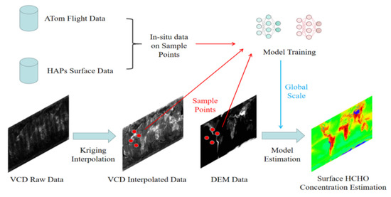
Figure 1.
Data processing workflow.
2.1. Datasets
2.1.1. Sentinel-5P VCD Data
The data on vertical column density (VCD) of HCHO in this study comes from TROPOMI (Tropospheric Monitoring Instrument), which is carried on Sentinel-5P [18,38]. Sentinel-5P is a global air pollution monitoring satellite launched by the ESA on 13 October 2017 as part of the Copernicus project. TROPOMI can effectively observe trace gas components in the atmosphere around the world, including NO2, O3, SO2, HCHO, CH4, CO and other important indicators closely related to human activities, and can strengthen the observation of aerosols and clouds [39].
In terms of accuracy, TROPOMI is currently the most advanced atmospheric monitoring spectrometer, with the highest spatial resolution. The satellite provides global coverage daily with a spatial resolution of 5.5 km × 3.5 km and an equator crossing time at about 13:30 local time, which effectively ensures the comparability of data in different regions [17]. Sentinel-5P data are currently available for public access (https://s5phub.copernicus.eu/dhus/#/home accessed on 21 June 2021). The averaged uncertainty of TROPOMI VCD HCHO data is 1.2 × 10¹⁶ molec.cm−2 (80%) [40], and the method used for the derivation of HCHO VCD from UV spectral measurements is the Differential Optical Absorption Spectroscopy method [17].
We used the data for 2019 because (a) 2018 is the first year that Sentinel-5P was in operation, and the algorithm of the product was not as stable then; (b) 2020 was within the global COVID-19 pandemic, which might have had a special impact on anthropogenic sources, making the result less representative in terms of their long-term status.
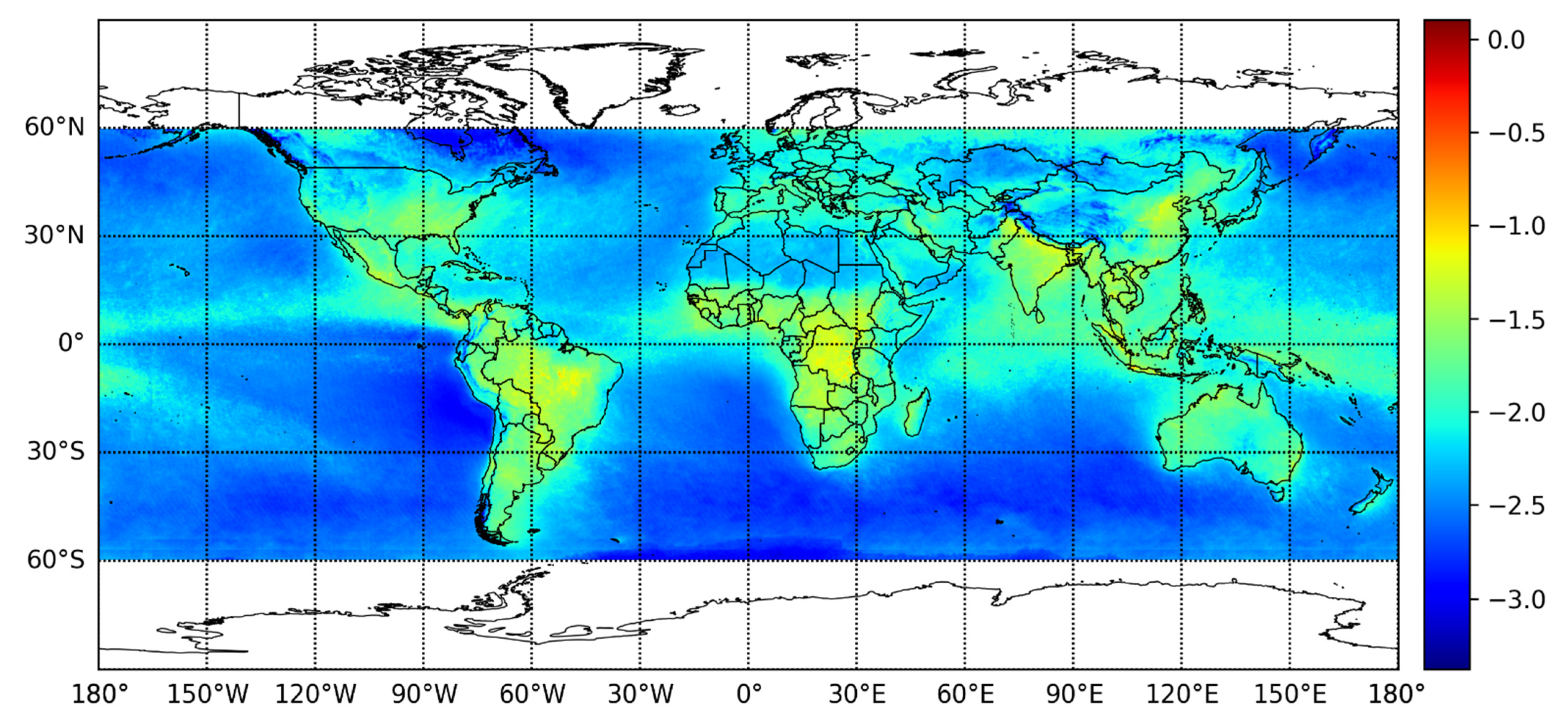
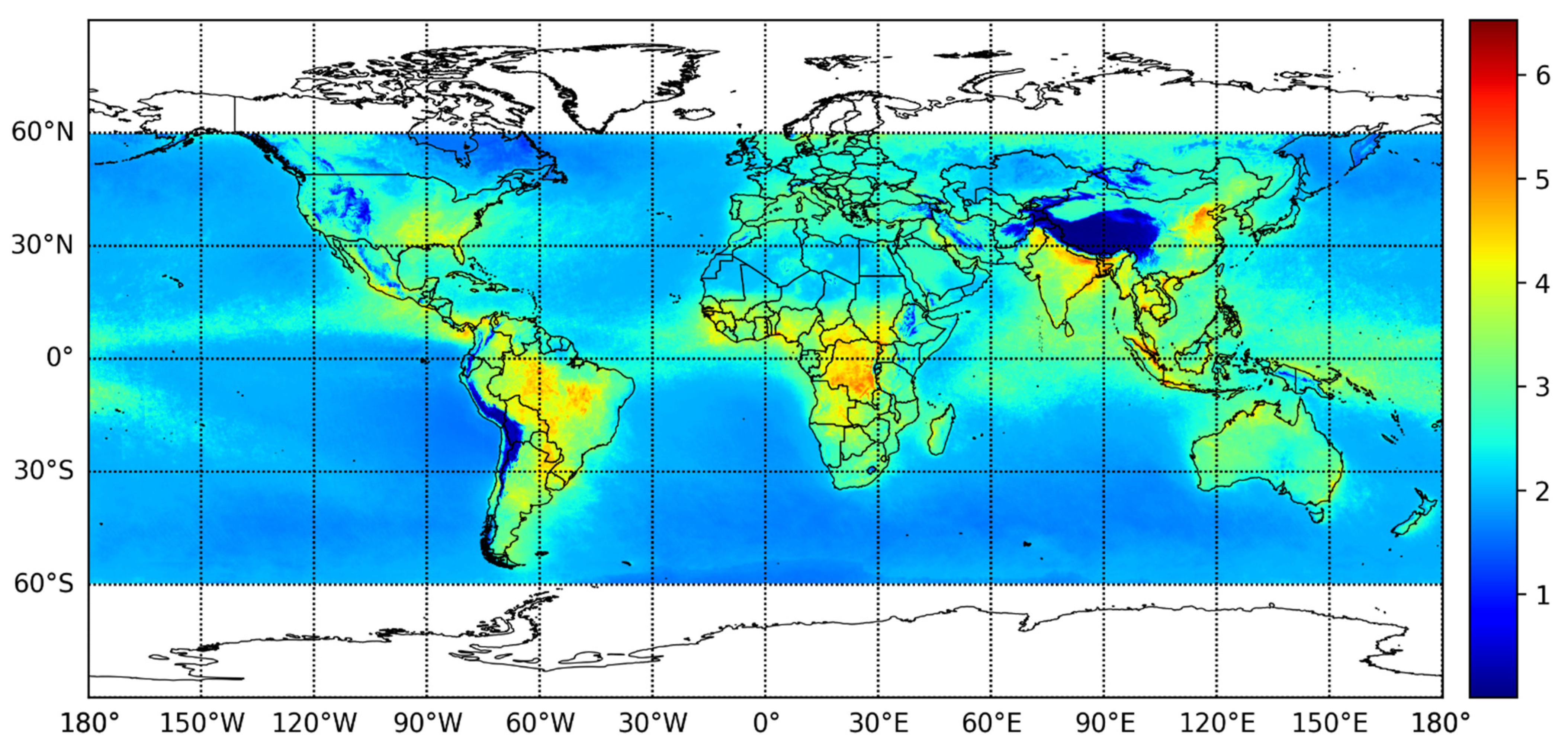
Offline HCHO data from 1 January to 31 December 2019 were collected. According to the technical documents, data points whose quality index (QA_value) was less than 0.5 were removed in order to ensure the best quality. After performing mosaic on the datasets and applying Ordinary Kriging interpolation, we obtained the distribution of global average total column concentration of HCHO with a resolution of 0.05° by 0.05° (Figure 2). The data beyond 60° S and 60° N were discarded due to the sparsity of satellite data and scarceness of human activities, which has little impact on health risk estimation.
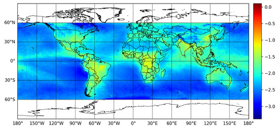
Figure 2.
The natural logarithm of global vertical column density (VCD) of HCHO in 2019, after being interpolated and averaged on an annual basis. (unit: mol/m2).
2.1.2. In-Situ Data
Since our study aimed to estimate the surface concentration of HCHO on a global level, we needed surface-level concentration data covering diverse types of underlying surfaces as well as different altitudes in order to train our model. Therefore, the following two data sources were considered.
ATom aerial in-situ data. NOAA/NASA’s atmospheric tomography mission (ATom) is a systematic global sampling of the atmosphere in the United States from 2016 to 2018, and provides continuous profile analysis from 0.2 km to 12 km. The volume mixing ratio of HCHO in air was provided by ATom flight measurements. A large number of gases and aerosol payloads were deployed on NASA’s DC-8 aircraft; among these, HCHO was measured by the ISAF instrument [41,42]. This instrument uses laser-induced fluorescence (LIF) to obtain the high sensitivity needed to detect HCHO in the upper troposphere and lower stratosphere, where it has an abundance of about ten parts per trillion. LIF can also achieve a quick response to measure the abundance of HCHO in the fine structure outflow of convective storms. These HCHO measurements can be used to elucidate the mechanism of convective transport and to quantify the effects of boundary layer pollutants on ozone photochemistry and cloud microphysics in the upper atmosphere [43]. Atom data are taken only once at quite arbitrary hours of the day. Since the ocean is relatively free from anthropogenic VOC sources, and since sea water buffers the air–sea VOC exchange at quite a steady rate (and which is quite hard to observe) [44,45], we assume that the diurnal VOC concentration variation can be ignored. Therefore, we took the Atom HCHO data as a diurnal average, since a remarkable percentage of HCHO comes from the secondary product of VOC oxidation [46].
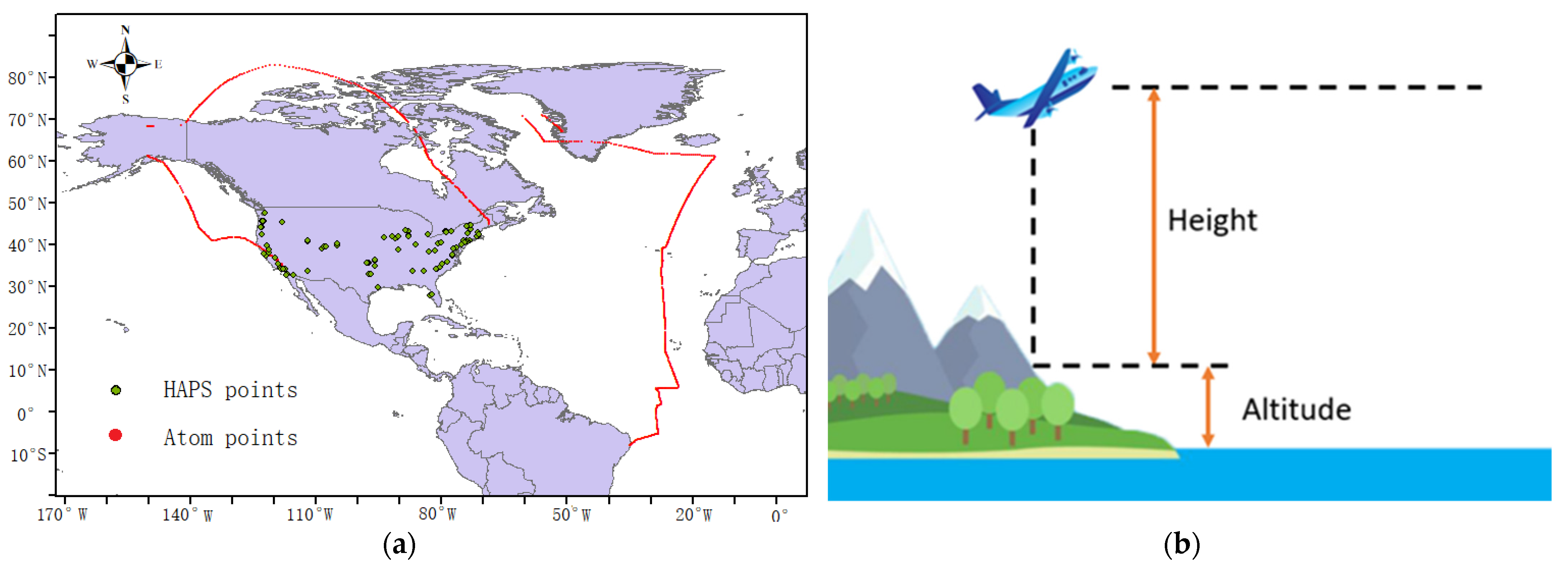
HAPs ground monitoring data. We obtained ground HCHO observations from EPA SLTS network at https://www.epa.gov/outdoor-air-quality-data accessed on 21 June 2021, which reports diurnal average HCHO concentration throughout the year. Here, we used 5965 data points from 109 sites in 2019, covering the whole country, as shown in Figure 3a.

Figure 3.
(a) The geographical distribution of our data, where red represents ATom aerial in-situ data points and green represents HAPs ground monitoring network. (b) The meaning of “Height” and “Altitude” for ATom mission data.
These two datasets generally represented the diurnal average HCHO level, and covered a wide range of latitudes from −8.1977° S to 82.9404° N as well as a diverse variety of landscapes in the U.S. The selection of the HAP dataset was to ensure that the concentration distribution feature at ground level was represented in our model, and the use of ATom data was to ensure that our model could be generalized and applied at the global scale.
Since ATom data are obtained far above the surface, and the vertical distribution of HCHO usually changes largely from ground to 1~2 km above [47], we took the “Height” of the aircraft measurements as another input variable in our model to control the impact of vertical distribution along the column. For HAPs ground in-situ data, we assigned 0 as the height.
Figure 4 illustrates how the in-situ data were matched up with the satellite data spatially. The circle represents the center of each pixel of satellite data, and the brown lines indicate the vertical projection of in-situ data. The in-situ data is matched with the nearest pixel center of a satellite data grid, as shown by the red arrows in Figure 4.
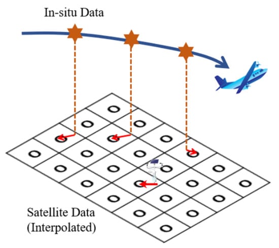
Figure 4.
Spatial matchups of in-situ data with satellite data.
2.1.3. Global DEM Data
Since descriptive statistics showed a negative relationship between surface altitude and in-situ concentration, with a Pearson’s correlation of r = −0.3907 in our in-situ dataset, we used global Digital Elevation Model (DEM) data as one of the input variables, “Altitude”, in order to estimate the ground-level concentration. The relationship between the variables “Height” and “Altitude” is shown in Figure 3b.
In our study, we used the Shuttle Radar Topography Mission (SRTM) DEM product and resampled it to a resolution of 0.05°. This dataset had an initial resolution of 90 m at the equator and was provided in WGS84 projection with a resolution of 1 arc [48].
2.2. Data Processing
After collecting and organizing data into formattable structure, we visualized and preprocessed these data. Then, two neural networks were implemented for point and interval estimations by using PyTorch, a well-known deep-learning framework. Our code is available online (https://github.com/dingyizhe2000/Interval-HCHO-Concentration-Estimation accessed on 21 June 2021).
The preprocessed data with the ground truth from in-situ HCHO concentration were then divided randomly into two groups; 90% of the dataset was used to train our models and 10% was used for validation. After that, global VCD data were fed into the model in order to derive global surface level HCHO concentration.
2.2.1. Preprocessing
In theory, a neural network is able to handle input data with a varied distribution; however, a significant defect was noticed in the training process without preprocessing, owing to the highly imbalanced and skewed distribution of the HCHO concentration (both column and in-situ). Therefore, we first applied log-transformation to the raw data. As shown in Figure S1, the logarithm of the HCHO concentration data shows a bell-shaped distribution, and increments in estimation accuracy have also proven the effectiveness of log-transformation.
2.2.2. Neural Network Architecture
As a universal function approximator, the neural network played a vital role in helping us derive the point and interval estimations of the HCHO concentration. However, instead of training a single network to get these estimations jointly, two separate neural networks were constructed for point and interval estimation, respectively, because several experiments which we carried out indicated that a joint model always has to compromise between point estimation and interval estimation, thus greatly reducing the accuracy of point estimation.
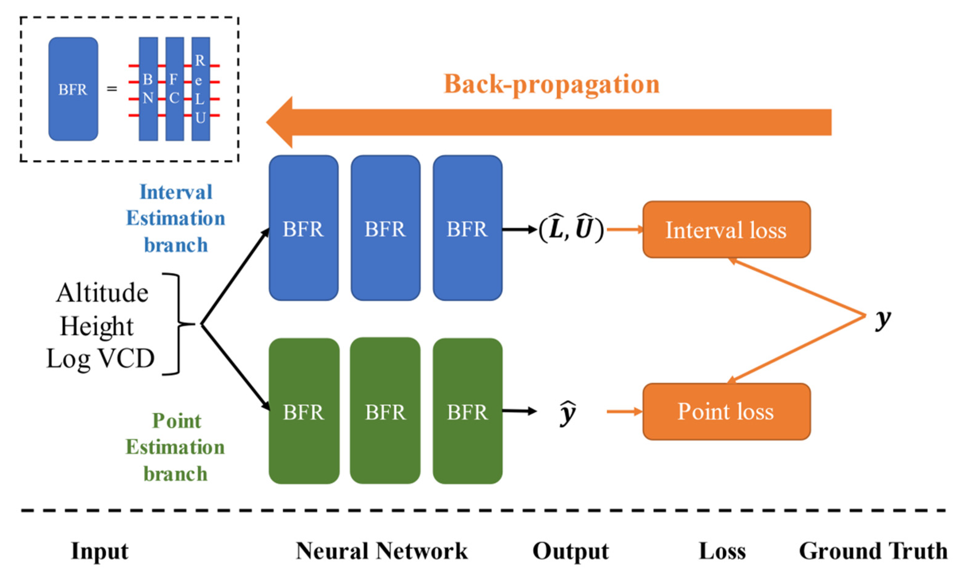
Like ordinary multi-layer perceptrons, each neural network in our model contained three input nodes, three BFR blocks (with the ReLUs in the last blocks disabled). The network for point estimation had one output node, and the other network for interval estimation had two nodes. The structure of our model is shown in Figure 5.

Figure 5.
Illustration of two separate neural networks for point and interval estimations respectively. Each network has three BFR blocks (with ReLU in the last block disabled).
For the sake of stabilizing the training and prediction procedure, instead of stacking full-connection and non-linear activation layers, we proposed to stack BFR blocks, which are made up of a batch normalization layer, a full connection layer and a ReLU activation layer sequentially.
Batch normalization (BN) was first introduced to address Internal Covariate Shift, a phenomenon referring to the unfavorable change of data distributions in the hidden layers. Just like data standardization, BN forces the distribution of each hidden layer to have exactly the same means and variances dimension-wise, which not only regularizes the network but also accelerates the training procedure by reducing the dependence of gradients on the scale of the parameters or of their initial values [49].
The full connection (FC) layer was connected immediately after the BN layer in order to provide linear transformation, where we set the number of hidden neurons as 50. The output from the FC layer was non-linearly activated by ReLU function [49,50]. The specific method is shown in the Supplemental materials.
2.2.3. Loss Function
Objective functions with suitable forms are crucial for applying stochastic gradient descent algorithms to converge while training. Though point estimation only needs to take precision into consideration, two conflicting factors are involved in evaluating the quality of interval estimation: higher confidence levels usually yield an interval with greater length, and vice versa.
With respect to point estimation loss, we found that dispensing with more elaborate forms, a loss is sufficient for training rapidly:
Interval estimation loss is relatively complex compared to point estimation loss. The QD-loss takes the confidential level and interval length into consideration simultaneously [37]:
On the one hand, in order to control the confidential level of the interval estimator, is set to indicate at most how many intervals proportionally failing to cover the true value can be tolerated. We set multiple , including 0.05, 0.10 and 0.20 in our model in order to derive interval predictions of various confidence levels and average coverage length, and it was verified that higher yields shorter intervals. indicates the covering rate of intervals:
where if and only if , else it equals 0.
On the other hand, the average length of intervals subject to should be minimized. However, intervals that fail to capture their corresponding data point should not be encouraged to shrink further. The average interval length to penalize is therefore
where works as a continuous approximation towards “hard”, since the sigmoid function is known for providing a differentiable alternative to discrete stepwise functions, and is a super-parameter for smoothness.
3. Results
3.1. Point Estimation
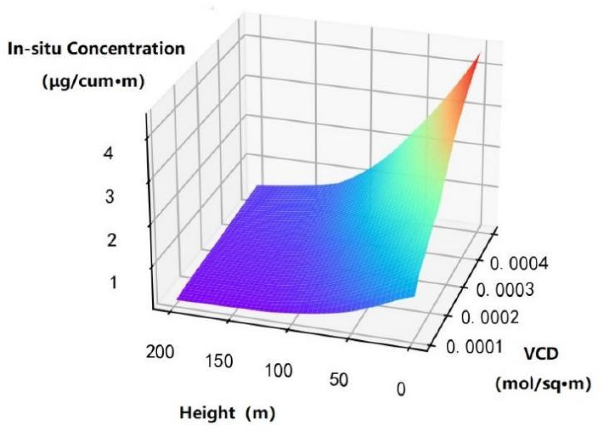
The point estimation model in this study showed relatively high accuracy and was generally consistent with previous studies on the vertical distribution of HCHO. Figure 6 shows the point estimation value of in-situ concentration with the change of vertical column density (VCD) and height when altitude at sea level is fixed. It can be seen that in-situ concentration is negatively correlated with height and positively correlated with VCD.

Figure 6.
The model’s estimation of in-situ concentrations of HCHO at certain height and vertical column densities when altitude is fixed at 0 m.
To evaluate the performance of our model, statistics including MAE and RMSE were calculated based on the training and validation datasets, respectively. As shown in Table 1, both MAEs and RMSEs were around 1μg/m3. As for relative bias, MAE to the average of surface concentration: was 0.495997 on the training set and 0.540923 on the validation set; RMSE to the average of surface concentration: was 0.390205 on the training set and 0.449029 on the validation set. Although the values seem to be somewhat high, they are in the same order of magnitude as the uncertainty of the TROPOMI data, which has a 40–80% bias with MAXDOS sites. In addition, this bias can be diluted by calculating long term averages during the process of deriving health risks.

Table 1.
MAE and RMSE of point estimation for surface concentration (unit: μg/m3).
By loading the global DEM, logarithm VCD and the height (0 m at surface) into the model, the annual average of the global surface HCHO distribution map was derived. As shown in Figure 7, there are generally six regions where HCHO surface concentration is high, namely the Amazon area, Southeastern U.S., Central and Western Africa, Northeastern India, South East Asia, and North China, with an average concentration of more than 4 μg/m3. The seasonal change of HCHO in these key areas is discussed in Section 3.3.
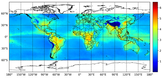
Figure 7.
Annual average of global surface concentration in 2019. (unit: μg/m3).
The uneven distribution of HCHO concentration on the sea and land surface is also noticeable in Figure 7, which shows that the HCHO concentration is relatively lower and more homogeneous on the sea surface than on the land. The statistics given in Table 2 also confirm this. It can be seen that the annual mean of surface HCHO concentration is about 2.21 μg/m3 over the ocean and 2.77 μg/m3 over land.
Table 2.
Statistics of surface HCHO concentration for sea surface, land surface and combined (unit: μg/m3).
Cities, as the regions with the densest population, deserve specific attention towards their surface HCHO concentration due to its known and potential harms to people living there. Table 3 shows the surface concentration of HCHO for some of the typical cities in these regions, with Jakarta and Singapore, two major cities in South East Asia, ranking the highest and the second highest with 6.18 and 5.83 μg/m3, respectively.
Table 3.
Surface HCHO concentration in some typical cities.
3.2. Interval Estimation
Besides point estimation, the model in this study also provided estimations of the upper and lower bounds of surface concentration of HCHO, so that the uncertainty, or variability of the surface concentration can be evaluated. In Figure 8a, the relationship between the estimated upper bound, lower bound and the point estimation are displayed in a 3D space. Figure 8b shows the results of cross-validation on the validation set. The point estimation lies around the red line, in the middle of the upper bound and lower bound (90% CI). It is worth emphasizing that the captured uncertainty, or the interval length, delineates the variability of the data itself, not the lower trustworthiness of our model or its estimations.
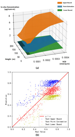
Figure 8.
(a) The estimated upper bound, point estimation and lower bound (90% CI) as a function of the height and vertical column density of HCHO when the altitude is fixed at 0 m, where CI represents confidence level. The results in this figure were obtained by feeding the equally spaced mock data into the two models. (b) The comparison of the models’ estimation and the real value in the validation set. Taken logarithm and standardized to 0–1 for proper visualization.
Confidence level, together with covering length, lay the foundation for the trustworthiness and precision of our interval prediction. As shown in Table 4, the interval estimation model obtained the covering rates and the ratio of true values covered by the predicted interval of 94.41% and 88.74%, exceeding the pre-set confidence levels of and , respectively.
Table 4.
Statistics of interval estimation for surface concentration (unit: μg/m3).
In addition, as expected in Section 2.2.3, a higher confidence level yielded a longer average interval length (Interval length = Upper Bound–Lower Bound), which was 4.530 μg /m3 for , 17% more than 3.864 μg /m3 for . Such a phenomenon can also be seen in the statistics, shown in Table 4, for minimum, maximum and mean values of the upper and lower bounds, respectively, for the two confidence levels.
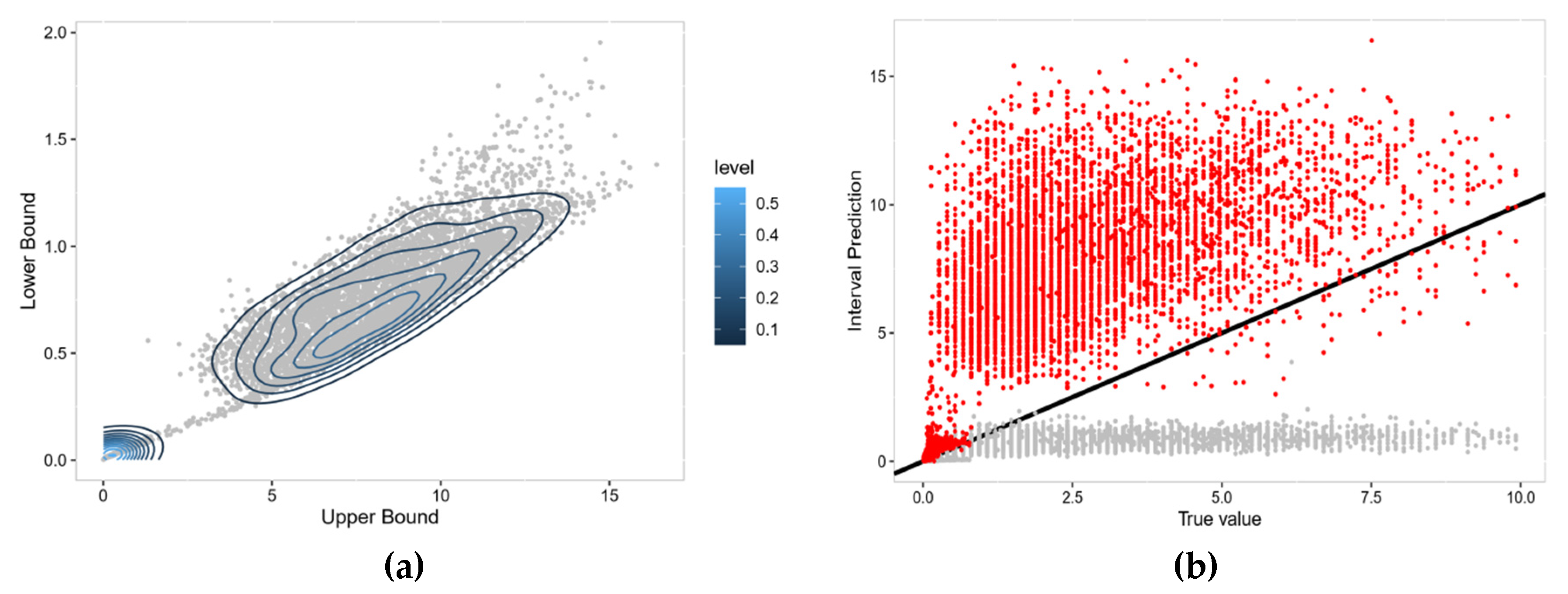
However, the standard deviation of upper bounds seems to be larger than that of the lower bounds under both scenarios in Table 4. From the density scatter plot between these two, shown in Figure 9, it can be seen that that the upper bound estimation is not deterministic, though interval estimation successfully covers the true values (and point estimations, as discussed below) of surface concentration. Nevertheless, further exploration of seasonal changes of HCHO in some key areas in Section 3.3 could explain that seasonal variations of surface HCHO may contribute to the majority of the uncertainty in interval estimation.
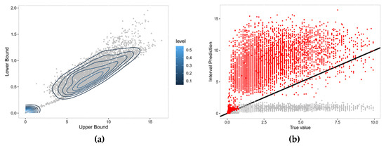
Figure 9.
(a) The density scatter plot of upper bound (x-axis) against lower-bound (y-axis). (b) Scatter plot of the relation between point estimation (x-axis) and predicted intervals (y-axis); red points are for upper bounds and grey points are for lower bounds. The black line is the fitted line. (unit: μg/m3).
Global distribution of the estimated upper and lower bounds is given in Figure 10a. It shows that the upper and lower bounds generally share the same global pattern, though with different magnitudes, with a range of between 3.77 and 8.83 μg/m3 for upper bounds and from 0.52 to 1.03 μg/m3 for lower bounds. The interval length6 of 90% confidence interval is 4.77 μg/m3.
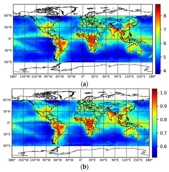
Figure 10.
(a) Distribution of upper bound from 90% surface concentration estimation. (b) Distribution of lower bound from 90% surface concentration estimation. (unit: μg/m3).
As shown in Figure 10b, the upper and lower bounds share a significantly positive relation, and a majority of predicted intervals are in the regions of 0.5~1.0 μg/m3 for lower bounds and 5~10 μg/m3 for upper bounds. aims for indicating the relative positions of true values in the predicted intervals. In addition, the predicted intervals can essentially cover true values.
3.3. Seasonal Changes of HCHO in Some Key Regions
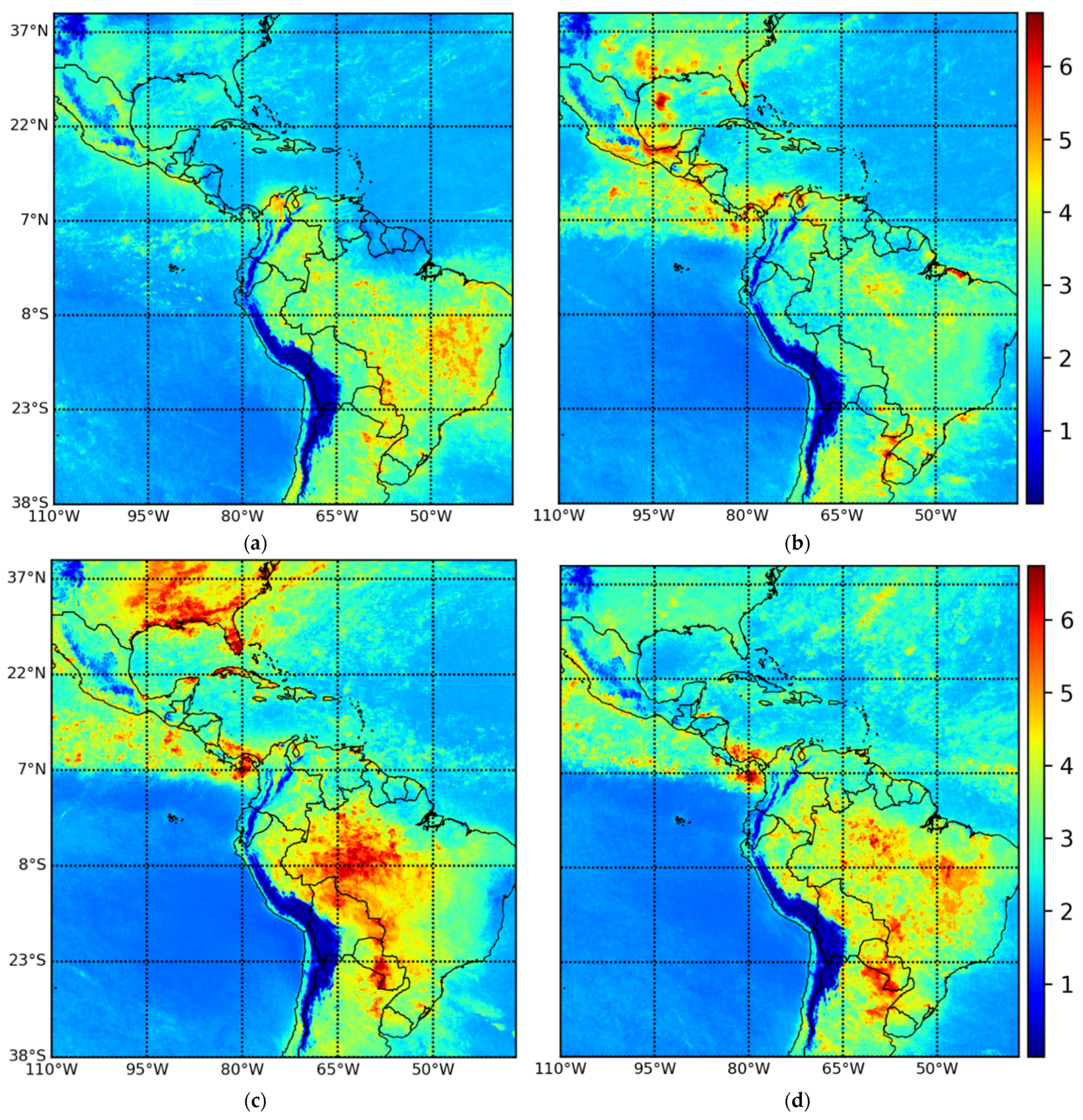
To better understand the seasonal variation of surface HCHO, the distribution pattern of four typical months of some key areas where surface concentration is relatively high were analyzed.
America.Figure 11 shows the surface concentration in February, May, August, and November in South America and around the Caribbean Sea. The Amazon Basin, Paraguay, and Eastern Central America had a high HCHO surface concentration in May and August, which is attributed to the large number of tropical rain forests and HCHO released by biomass combustion in the dry season [51]. In addition, the southeastern coast of the U.S. had the highest concentration in August and was almost free from HCHO pollution in February and November, which may be because plants are more active and release more volatile organic compounds (VOCs), particularly biogenic isoprene, during the summer [46]. The Andes Mountains had a significantly low concentration, with a value of less than 0.5 μg/m3.
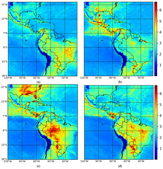
Figure 11.
Surface concentration of HCHO in Central and South America in some typical months: (a) February; (b) May; (c) August; (d) November. (unit: μg/m3).
Africa. As shown in Figure 12, there are two regions in Africa whose HCHO surface concentration is relatively high. One is in the south of R. D. Congo around the city of Kolwezi, a mining center with a humid subtropical climate. The surface concentration of HCHO here reaches its maximum in July. The other pollution belt stretches along the Gulf of Guinea, which is famous for its rainforest climate. Oxidation of biological isoprene released from tropical rain forest and biomass burning are the main cause of formaldehyde pollution [52,53].
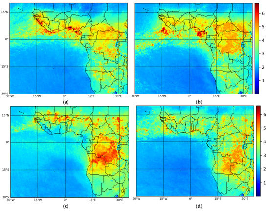
Figure 12.
Surface concentration of HCHO in Central and South Africa in some typical months: (a) January; (b) April; (c) July; (d) October. (unit: μg/m3).
Indo-Pacific. As shown in Figure 13, there are several regions in the Indo-Pacific where the timing of high HCHO concentrations differ from each other; this may result from several different reasons. First, Malaysia and the Indonesian islands, due to their large number of tropical rain forests, have relatively high concentrations all the year round and reach their maximum in December [54]. Second, the surface HCHO concentration of the China-Indochina Peninsula reach their maximum in March, while the high concentration center moves to the Gulf of Tonkin and Pearl River Delta in June. Third, the Bay of Bengal and the coasts nearby witness a high concentration in September. Fourth, the Beijing-Tianjin-Hebei Urban Agglomeration (BTH) has no rainforest distribution but mass population and economic activities, which contribute to a high HCHO concentration through most of the year [55]. The concentration there reached its maximum in 2019 around September.
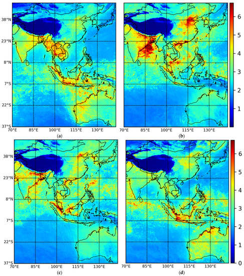
Figure 13.
Surface concentration of HCHO in Indo-Pacific region in some typical months: (a) March; (b) June; (c) September; (d) December. (unit: μg/m3).
4. Discussion
4.1. Improvements and Innovativeness
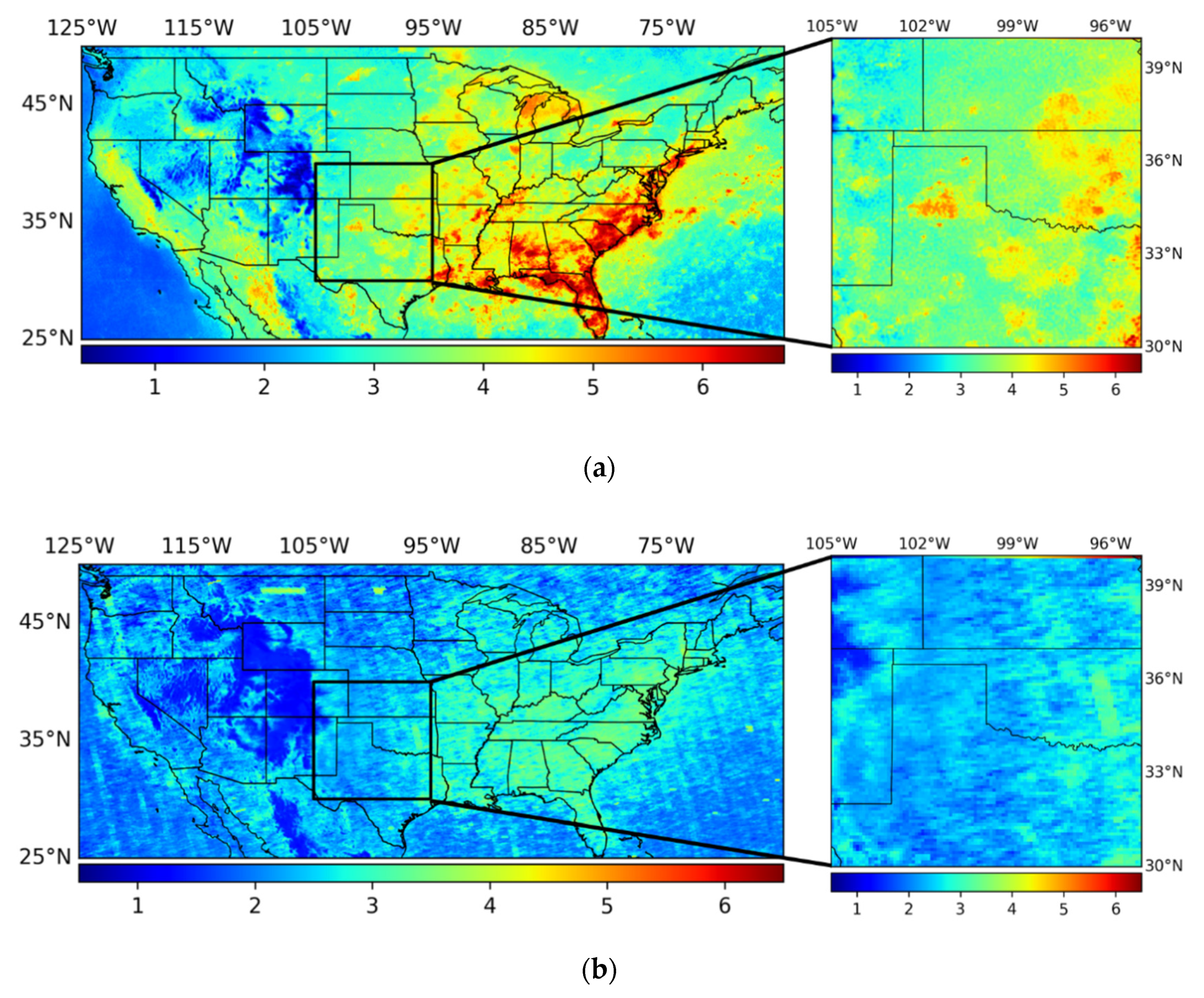
It is clear that the global surface distribution of HCHO with point and interval estimation is able to be obtained successfully by using neural network models like those described above. To show the improvement of Sentinel-5P in pollutant health estimation, the point estimation model was applied to both Sentinel-5P VCD data and OMI VCD data for July 2019. Zooming in on the view of America, two things can be seen from the comparison.
First, Sentinel-5P is far less disturbed by noise along the satellite trail. This was precisely the goal of the designers of Sentinel-5P before its launch [56]. The improvement of signal-to-noise ratio in TROPOMI is well illustrated by Figure 14.

Figure 14.
(a) Average surface distribution of HCHO over the U.S. in July 2019, derived from Sentinel-5P data; (b) Average surface distribution of HCHO over the U.S. in July 2019, derived from OMI data (unit: μg/m3).
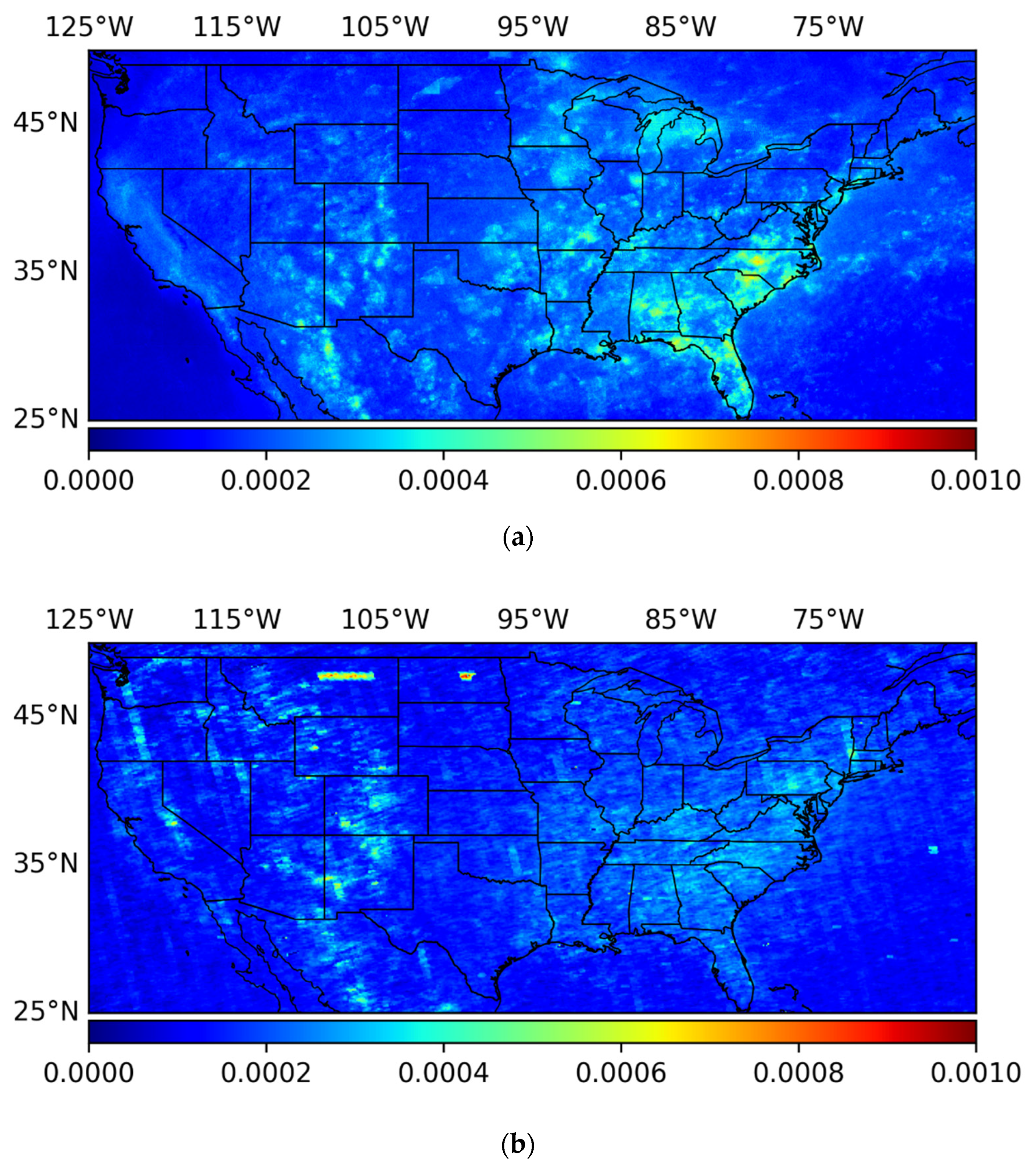
Second, although Sentinel-5P and OMI generally give the same distribution trend, Sentinel-5P shows an obviously higher level of HCHO. This can be attributed to the slightly higher concentration levels in VCD data, as is shown in Figure 15. In shown area, due to the non-linear character of the model, a 17.8% higher observed VCD level leads to a 42.2% higher level of surface HCHO estimation, which would make a huge difference to further health risk estimation. Therefore, the high sensitivity of the model requires very precise HCHO VCD observation. This phenomenon calls for more studies on the validation between TROPOMI and OMI.

Figure 15.
(a) Average HCHO VCD over the U.S. in July 2019, derived from Sentinel-5P data; (b) Average HCHO VCD over the U.S. in July 2019, derived from OMI data (unit: mol/m2).
The results of global surface concentration estimation for 2019 give a closer look at the global distribution pattern of HCHO. Obviously, HCHO tends to prevail on the plain of the continent, instead of over the oceans or in high altitude areas. According to previous studies, this can be attributed to the scarceness of VOC sources such as chemical industry, combustion, and rainforests, which are common precursors of the free radical reaction of HCHO production [57,58,59]. By mapping the distribution of HCHO, two kinds of sources around the world can be distinguished preliminarily. One is plant-related, including the Amazon, South East Asia, and the Gulf of Guinea; the other is human-related, including the North China Plain and Pearl River Delta [60,61]. More work is needed to accurately identify the source of these HCHO-polluted areas.
In addition, we introduce here for the first time interval estimation using the neural network model for the conversion from VCD to global surface concentration of HCHO, increasing the credibility of the model by providing uncertainty information. This new idea can make up for the deficiency of inexplicability of the neural network model [62], thus being useful for the application of neural network models in the field of estimating atmospheric pollutants or health risk in the future.
4.2. Limitations and Potential Improvements
Despite the improvements and innovativeness mentioned before, the shortage of in-situ data hinders the further improvement of model accuracy. On one hand, the existing HCHO in-situ concentration data is seriously insufficient in both the spatial and temporal dimensions. Only the U.S. monitors HCHO in-situ concentration routinely, mostly in urban areas. Even if ATom data are also adopted, in-situ concentration data in low latitude regions and rural areas is still sparse, which may lead to estimation bias in the regions outside urban America. On the other hand, it is also difficult to reach a better result by adding more covariates into our model. Experiments with additional covariate inputs such as latitude and months have failed, with degenerated or overfitting outputs. In addition, the large gap between true values and the upper bounds from our interval estimation model may suggest a heterogeneous in-situ concentration of HCHO distribution in different months or seasons, since the model is required to give the interval estimations on the scale of a whole year, rather than on a fine time scale. The seasonal changes of HCHO in some key areas, as discussed in Section 3.3, have also demonstrated this phenomenon directly.
Good agreement shown in the validation over North America indicated the capability of the framework of the model we designed; uncertainties will be well under-controlled and improved once more training datasets covering other part of the world and other time periods become available in the future as rendered by ongoing and future satellite missions and also by increased ground-based monitoring activities. Meanwhile, with more Sentinel-5P data accumulating over time, the model in this study can take more factors such as latitude and seasons into consideration, which could provide more precise estimation of global-scale health risks and economic loss based on specific regions and seasons. Besides the significance of the health risks, the results from this study can also aid research on the generation of photochemical pollution, the concentration of VOCs, NO2 and other photochemical reaction-related pollutants.
4.3. Health Risk of HCHO in Major Cities
HCHO, as one of the most important carcinogens in the outdoor environment [2], draws little attention due to the longtime lack of ground measurement of HCHO in most countries and regions, leading to a shortage of knowledge about resulting health and economic losses. Even if the vertical column density of HCHO is currently available and does partially settle concerns about these issues, it is the ground level HCHO concentration that reflects the actual amount of concentration people are exposed to.
Taking 2019 as an example, it was assumed that the HCHO concentration has always been the same as that year. Health risks were calculated using inhalation unit risk and population data [4,63] (the specific method is shown in the Supplementary materials). Health risks in the main high-risk cities were calculated and are given in Table 5. It is indicated that more than a thousand people have the potential to get cancer due to exposure to HCHO in Jakarta, Dhaka, Bangkok, Kolkata, Beijing and Guangzhou. Jakarta has the most potential victims of exposure, with 2593. Jakarta, Singapore, Kuala Lumpur, Dhaka and Lagos are the cities with the highest prevalence of exposure, with 80.34, 75.79, 72.93, 71.63, and 71.37 potential cancer patients per million, respectively. The main cities with high health risks are concentrated in Southeast Asia, which has been previously neglected by academia but which may become the next hotspot for research into HCHO pollution and the attendant health risk.
Table 5.
Potential number of cancer cases in typical cities if HCHO surface concentration remains at 2019 levels.
5. Conclusions
With the benefit of a quality-driven interval estimation algorithm designed for neural networks, we were able to derive confidence intervals and a precise point estimation of 2019 global surface HCHO at different confidence levels, even with a limited amount of data. By mapping the HCHO surface concentration distribution, we found that Southeast Asia, North China, Central and Western Africa, and the rainforest area of Latin America have relatively more serious HCHO pollution than other regions. Major cities in these regions, such as Bangkok, Beijing, Guangzhou and Singapore, have an annual concentration over 5.00 μg/m3. The health effects from such high levels of HCHO pollution deserve more attention from academia and governments.
Our work paves the way for research on formaldehyde-related cancers and provides guidance for policymaking and insurance pricing. To the best of our knowledge, we are the first to map the global distribution of HCHO and provide insights on its potential health risks. With more HCHO VCD data from Sentinel-5P accumulating, the surface concentration of HCHO dataset covering a longer period of time will be generated, which will aid in better assessment of the global risk distribution of formaldehyde-related cancers.
Supplementary Materials
The following are available online at https://www.mdpi.com/article/10.3390/rs13204055/s1, Figure S1. (a) Distribution of vertical column density (mmol/sq·m); (b) Distribution of log (vertical column density); (c) Distribution of log (in-situ concentration); (d) Distribution of in-situ concentration (μg/cum·m), Method 1. Health Risk, Method 2. Neural Network Architecture.
Author Contributions
Conceptualization, W.W.; Methodology, J.G. and Y.D.; Software, J.G., G.L., B.J. and Y.D.; Validation, B.J.; Formal Analysis, J.G. and B.J.; Investigation, B.J. and J.G.; Resources, B.J. and J.G.; Data Curation, B.J. and Y.D.; Writing, J.G., B.J., Y.D. and P.C.; Visualization, B.J. and Y.D.; Supervision, W.W. and P.C.; Project Administration, W.W.; Funding Acquisition, W.W. All authors have read and agreed to the published version of the manuscript.
Funding
This research was supported by the National Social Science Foundation of China Grant (16CTJ003).
Data Availability Statement
The data presented in this study are openly available at https://s5phub.copernicus.eu/dhus/#/home (accessed on 21 June 2021) for Sentinel-5P VCD Data; https://www.epa.gov/outdoor-air-quality-data (accessed on 21 June 2021) for HAPs ground in-situ data; https://drive.google.com/drive/folders/0B_J08t5spvd8VWJPbTB3anNHamc (accessed on 21 June 2021) for Global DEM Data. ATom aerial in-situ data is available in a publicly accessible repository [40,41]. The input data of our model is available at [https://drive.google.com/file/d/1tovF73HogGNEXC1i_jBbnVRHlm1n-ZT_/view?usp=sharing (accessed on 21 June 2021)]. The data presented in this study are available at [https://drive.google.com/file/d/10A2VIEHm22DF_gyCufV-pbgUdYYhNJKf/view?usp=sharing (accessed on 21 June 2021)].
Acknowledgments
We appreciate Lei Zhu for providing us with technical support about searching available data. We also appreciate NOAA/NASA for their valuable Atmospheric Tomography Mission data, US EPA for the ground-based measurements and ESA for its TROPOMI VCD HCHO data.
Conflicts of Interest
The authors declare no conflict of interest.
References
- Tesfaye, S.; Hamba, N.; Gerbi, A.; Neger, Z. Oxidative Stress and Carcinogenic Effect of Formaldehyde Exposure: Systematic Review & Analysis. Endocrinol. Metab. Syndr. 2020, 9, 319. [Google Scholar]
- Scheffe, R.D.; Strum, M.; Phillips, S.B.; Thurman, J.; Eyth, A.; Fudge, S.; Morris, M.; Palma, T.; Cook, R. Hybrid Modeling Approach to Estimate Exposures of Hazardous Air Pollutants (HAPs) for the National Air Toxics Assessment (NATA). Environ. Sci. Technol. 2016, 50, 12356–12364. [Google Scholar] [CrossRef] [PubMed]
- Blair, A.; Saracci, R.; Stewart, P.A.; Hayes, R.; Shy, C. Epidemiologic evidence on the relationship between formaldehyde exposure and cancer. Scand. J. Work. Environ. Health 1990, 16, 381–393. [Google Scholar] [CrossRef] [PubMed]
- Agency, E.P. Formaldehyde. Available online: https://www.epa.gov/sites/production/files/2016-09/documents/formaldehyde.pdf (accessed on 21 May 2021).
- Jin, X.; Fiore, A.; Boersma, K.F.; Smedt, I.D.; Valin, L. Inferring Changes in Summertime Surface Ozone–NO x–VOC Chemistry over US Urban Areas from Two Decades of Satellite and Ground-Based Observations. Environ. Sci. Technol. 2020, 54, 6518–6529. [Google Scholar] [CrossRef] [PubMed]
- Javed, Z.; Liu, C.; Khokhar, M.F.; Tan, W.; Liu, H.; Xing, C.; Ji, X.; Tanvir, A.; Hong, Q.; Sandhu, O.; et al. Ground-Based MAX-DOAS Observations of CHOCHO and HCHO in Beijing and Baoding, China. Remote Sens. 2019, 11, 1524. [Google Scholar] [CrossRef] [Green Version]
- Liu, Y.; Tang, Z.; Abera, T.; Zhang, X.; Hakola, H.; Pellikka, P.; Maeda, E. Spatio-temporal distribution and source partitioning of formaldehyde over Ethiopia and Kenya. Atmos. Environ. 2020, 237, 117706. [Google Scholar] [CrossRef]
- Kaiser, J.; Wolfe, G.M.; Bohn, B.; Broch, S.; Fuchs, H.; Ganzeveld, L.N.; Gomm, S.; Häseler, R.; Hofzumahaus, A.; Holland, F.; et al. Evidence for an unidentified non-photochemical ground-level source of formaldehyde in the Po Valley with potential implications for ozone production. Atmos. Chem. Phys. Discuss. 2015, 15, 1289–1298. [Google Scholar] [CrossRef] [Green Version]
- Green, J.R.; Fiddler, M.N.; Fibiger, D.L.; McDuffie, E.E.; Aquino, J.; Campos, T.; Shah, V.; Jaeglé, L.; Thornton, J.A.; DiGangi, J.P.; et al. Wintertime Formaldehyde: Airborne Observations and Source Apportionment Over the Eastern United States. J. Geophys. Res. Atmos. 2021, 126, e2020JD033518. [Google Scholar] [CrossRef]
- Geddes, J. Impacts of Interannual Variability in Biogenic VOC Emissions Near Transitional Ozone Production Regimes. In AGU Fall Meeting Abstracts; American Geophysical Union: Washington, DC, USA, 2017; p. A54B-06. [Google Scholar]
- Gratsea, M.; Vrekoussis, M.; Richter, A.; Wittrock, F.; Schönhardt, A.; Burrows, J.; Kazadzis, S.; Mihalopoulos, N.; Gerasopoulos, E. Slant column MAX-DOAS measurements of nitrogen dioxide, formaldehyde, glyoxal and oxygen dimer in the urban environment of Athens. Atmos. Environ. 2016, 135, 118–131. [Google Scholar] [CrossRef]
- EPA. Outdoor Air Quality Data. Available online: https://www.epa.gov/outdoor-air-quality-data (accessed on 21 March 2021).
- Product User Manual for GOME Total Columns of Ozone, NO2, Tropospheric NO2, BrO, SO2, H2O, HCHO, OClO, and Cloud Properties. Available online: https://atmos.eoc.dlr.de/app/docs/DLR_GOME_PUM.pdf (accessed on 1 October 2021).
- Algorithm Theoretical Basis Document for GOME-2 Total Column Products of Ozone, NO2, BrO, HCHO, SO2, H2O and Cloud Properties. Available online: https://atmos.eoc.dlr.de/app/docs/DLR_GOME-2_ATBD_GDP48.pdf (accessed on 1 October 2021).
- SCIAMACHY Offline Processor Level1b-2 ATBD Algorithm Theoretical Baseline Document. Available online: https://atmos.eoc.dlr.de/sciamachy/documents/level_1b_2/sciaol1b2_atbd_master.pdf (accessed on 15 September 2021).
- OMI Algorithm Theoretical Basis Document. Available online: https://ozoneaq.gsfc.nasa.gov/media/docs/ATBD-OMI-04.pdf (accessed on 15 September 2021).
- S5P/TROPOMI HCHO ATBD. Available online: https://sentinels.copernicus.eu/documents/247904/2476257/Sentinel-5P-ATBD-HCHO-TROPOMI (accessed on 15 September 2021).
- Veefkind, J.; Aben, I.; McMullan, K.; Förster, H.; de Vries, J.; Otter, G.; Claas, J.; Eskes, H.; de Haan, J.; Kleipool, Q.; et al. TROPOMI on the ESA Sentinel-5 Precursor: A GMES mission for global observations of the atmospheric composition for climate, air quality and ozone layer applications. Remote Sens. Environ. 2012, 120, 70–83. [Google Scholar] [CrossRef]
- Millet, D.B.; Jacob, D.J.; Boersma, K.F.; Fu, T.; Kurosu, T.P.; Chance, K.; Heald, C.L.; Guenther, A. Spatial distribution of isoprene emissions from North America derived from formaldehyde column measurements by the OMI satellite sensor. J. Geophys. Res. 2008, 113. [Google Scholar] [CrossRef]
- Zhang, Y.; Li, R.; Min, Q.; Bo, H.; Fu, Y.; Wang, Y.; Gao, Z. The controlling factors of atmospheric formaldehyde (HCHO) in Amazon as seen from satellite. Earth Space Sci. 2019, 6, 959–971. [Google Scholar] [CrossRef] [Green Version]
- Curci, G.; Palmer, P.I.; Kurosu, T.P.; Chance, K.; Visconti, G. Estimating European volatile organic compound emissions using satellite observations of formaldehyde from the Ozone Monitoring Instrument. Atmos. Chem. Phys. Discuss. 2010, 10, 11501–11517. [Google Scholar] [CrossRef] [Green Version]
- Biswas, M.S.; Choudhury, A.D. Impact of COVID-19 Control Measures on Trace Gases (NO2, HCHO and SO2) and Aerosols over India during Pre-monsoon of 2020. Aerosol Air Qual. Res. 2021, 20, 200306. [Google Scholar] [CrossRef]
- Sun, W.; Zhu, L.; De Smedt, I.; Bai, B.; Pu, D.; Chen, Y.; Shu, L.; Wang, D.; Fu, T.; Wang, X.; et al. Global Significant Changes in Formaldehyde (HCHO) Columns Observed From Space at the Early Stage of the COVID-19 Pandemic. Geophys. Res. Lett. 2021, 48, 2e020GL091265. [Google Scholar] [CrossRef] [PubMed]
- Yu, T.; Wang, W.; Ciren, P.; Zhu, Y. Assessment of human health impact from exposure to multiple air pollutants in China based on satellite observations. Int. J. Appl. Earth Obs. Geoinf. 2016, 52, 542–553. [Google Scholar] [CrossRef]
- Schroeder, J.R.; Crawford, J.H.; Fried, A.; Walega, J.; Weinheimer, A.; Wisthaler, A.; Müller, M.; Mikoviny, T.; Chen, G.; Shook, M.; et al. Formaldehyde column density measurements as a suitable pathway to estimate near-surface ozone tendencies from space. J. Geophys. Res. Atmos. 2016, 121, 13088–13112. [Google Scholar] [CrossRef] [Green Version]
- Zhu, L.; Jacob, D.J.; Keutsch, F.N.; Mickley, L.J.; Scheffe, R.; Strum, M.; Abad, G.G.; Chance, K.; Yang, K.; Rappenglück, B.; et al. Formaldehyde (HCHO) As a Hazardous Air Pollutant: Mapping Surface Air Concentrations from Satellite and Inferring Cancer Risks in the United States. Environ. Sci. Technol. 2017, 51, 5650–5657. [Google Scholar] [CrossRef] [PubMed]
- Krizhevsky, A.; Sutskever, I.; Hinton, G.E. ImageNet classification with deep convolutional neural networks. Commun. ACM 2017, 60, 84–90. [Google Scholar] [CrossRef]
- Ren, S.; He, K.; Girshick, R.; Sun, J. Faster R-CNN: Towards Real-Time Object Detection with Region Proposal Networks. IEEE Trans. Pattern Anal. Mach. Intell. 2017, 39, 1137–1149. [Google Scholar] [CrossRef] [Green Version]
- Zhang, K.; Zuo, W.; Chen, Y.; Meng, D.; Zhang, L. Beyond a Gaussian Denoiser: Residual Learning of Deep CNN for Image Denoising. IEEE Trans. Image Process. 2017, 26, 3142–3155. [Google Scholar] [CrossRef] [PubMed] [Green Version]
- Goodfellow, I.; Pouget-Abadie, J.; Mirza, M.; Xu, B.; Warde-Farley, D.; Ozair, S.; Courville, A.; Bengio, Y. Generative Adversarial Nets. Adv. Neural Inf. Process. Syst. 2014, 27, 1–9. [Google Scholar]
- Ye, M.; Shen, J.; Lin, G.; Xiang, T.; Shao, L.; Hoi, S.C. Deep Learning for Person Re-identification: A Survey and Outlook. IEEE Trans. Pattern Anal. Mach. Intell. 2021. [Google Scholar] [CrossRef]
- Mackay, D.J.C. A Practical Bayesian Framework for Backpropagation Networks. Neural Comput. 1992, 4, 448–472. [Google Scholar] [CrossRef]
- Tibshirani, R. A Comparison of Some Error Estimates for Neural Network Models. Neural Comput. 1996, 8, 152–163. [Google Scholar] [CrossRef]
- Heskes, T.M.; Wiegerinck, W.; Kappen, H.J. Practical confidence and prediction intervals. Prog. Neural Process. 1997, 128–135. [Google Scholar] [CrossRef]
- Gal, Y.; Ghahramani, Z. Dropout as a Bayesian Approximation: Representing Model Uncertainty in Deep Learning. In Proceedings of the International Conference on Machine Learning, New York, NY, USA, 19 June 2016; pp. 1050–1059. [Google Scholar]
- Khosravi, A.; Nahavandi, S.; Creighton, D.; Atiya, A.F. Lower Upper Bound Estimation Method for Construction of Neural Network-Based Prediction Intervals. IEEE Trans. Neural Netw. 2010, 22, 337–346. [Google Scholar] [CrossRef]
- Pearce, T.; Zaki, M.; Brintrup, A.; Neely, A. High-Quality Prediction Intervals for Deep Learning: A Distribution-Free, Ensembled Approach. In Proceedings of the 35th International Conference on Machine Learning, Stockholm, Sweden, 10 July 2018; pp. 4075–4084. [Google Scholar]
- Sentinel-5 Precursor/TROPOMI Level 2 Product User Manual Formaldehyde HCHO. Available online: https://sentinels.copernicus.eu/documents/247904/2474726/Sentinel-5P-Level-2-Product-User-Manual-Formaldehyde (accessed on 1 October 2021).
- Sentinel-5 Precursor/TROPOMI Level 2 Product User Manual Carbon Monoxide Document Number. Available online: http://www.tropomi.eu/sites/default/files/files/Sentinel-5P-Level-2-Product-User-Manual-Carbon-Monoxide_v1.00.02_20180613.pdf (accessed on 1 October 2021).
- S5P Mission Performance Centre Formaldehyde [L2_HCHO] Readme. Available online: https://sentinels.copernicus.eu/documents/247904/3541451/Sentinel-5P-Formaldehyde-Readme.pdf (accessed on 15 September 2021).
- Williamson, C.; Kupc, A.; Wilson, J.; Gesler, D.W.; Reeves, J.M.; Erdesz, F.; McLaughlin, R.; Brock, C.A. Fast time response measurements of particle size distributions in the 3–60 nm size range with the nucleation mode aerosol size spectrometer. Atmos. Meas. Tech. 2018, 11, 3491–3509. [Google Scholar] [CrossRef] [Green Version]
- Brock, C.A.; Williamson, C.; Kupc, A.; Froyd, K.D.; Erdesz, F.; Wagner, N.; Richardson, M.; Schwarz, J.P.; Gao, R.-S.; Katich, J.M.; et al. Aerosol size distributions during the Atmospheric Tomography Mission (ATom): Methods, uncertainties, and data products. Atmos. Meas. Tech. 2019, 12, 3081–3099. [Google Scholar] [CrossRef] [Green Version]
- ATom: L2 Measurements of In-Situ Airborne Formaldehyde (ISAF). Available online: https://daac.ornl.gov/ATOM/guides/ATom_ISAF_Instrument_Data.html (accessed on 1 October 2021). [CrossRef]
- Fischer, E.V.; Jacob, D.J.; Millet, D.B.; Yantosca, R.M.; Mao, J. The role of the ocean in the global atmospheric budget of acetone. Geophys. Res. Lett. 2012, 39, L01807. [Google Scholar] [CrossRef] [Green Version]
- Singh, H.B.; Tabazadeh, A.; Evans, M.J.; Field, B.D.; Jacob, D.J.; Sachse, G.; Crawford, J.H.; Shetter, R.; Brune, W.H. Oxygenated volatile organic chemicals in the oceans: Inferences and implications based on atmospheric observations and air-sea exchange models. Geophys. Res. Lett. 2003, 30. [Google Scholar] [CrossRef]
- Palmer, P.I.; Jacob, D.J.; Fiore, A.M.; Martin, R.V.; Chance, K.; Kurosu, T.P. Mapping isoprene emissions over North America using formaldehyde column observations from space. J. Geophys. Res. Atmos. 2003, 108. [Google Scholar] [CrossRef] [Green Version]
- Wang, Y.; Dörner, S.; Donner, S.; Böhnke, S.; De Smedt, I.; Dickerson, R.R.; Dong, Z.; He, H.; Li, Z.; Li, Z.; et al. Vertical profiles of NO2, SO2, HONO, HCHO, CHOCHO and aerosols derived from MAX-DOAS measurements at a rural site in the central western North China Plain and their relation to emission sources and effects of regional transport. Atmos. Chem. Phys. Discuss. 2019, 19, 5417–5449. [Google Scholar] [CrossRef] [Green Version]
- Farr, T.G.; Edward, P.A.R.; Kobrick, M.; Rodriguez, M.P.E.; Shaffer, S.; Umland, J.S.J.; Burbank, D.; Alsdorf, A.D. The shuttle radar topography mission. Rev. Geophys. 2007, 45. [Google Scholar] [CrossRef] [Green Version]
- Ioffe, S.; Szegedy, C. Batch normalization: Accelerating deep network training by reducing internal covariate shift. In Proceedings of the International Conference on Machine Learning, Lille, France, 6 June 2015; pp. 448–456. [Google Scholar]
- Glorot, X.; Bordes, A.; Bengio, Y. Deep sparse rectifier neural networks. In Proceedings of the Fourteenth International Conference on Artificial Intelligence and Statistics, Fort Lauderdale, FL, USA, 11 April 2011; pp. 315–323. [Google Scholar]
- Barkley, M.P.; Kurosu, T.P.; Chance, K.; De Smedt, I.; Van Roozendael, M.; Arneth, A.; Hagberg, D.; Guenther, A. Assessing sources of uncertainty in formaldehyde air mass factors over tropical South America: Implications for top-down isoprene emission estimates. J. Geophys. Res. Space Phys. 2012, 117. [Google Scholar] [CrossRef]
- Meyer-Arnek, J.; Ladstätter-Weißenmayer, A.; Richter, A.; Wittrock, F.; Burrows, J.P. A study of the trace gas columns of O3, NO2 and HCHO over Africa in September 1997. Faraday Discuss. 2005, 130, 387–405. [Google Scholar] [CrossRef] [PubMed]
- Wittrock, F.; Richter, A.; Oetjen, H.; Burrows, J.P.; Kanakidou, M.; Myriokefalitakis, S.; Volkamer, R.; Beirle, S.; Platt, U.; Wagner, T. Simultaneous global observations of glyoxal and formaldehyde from space. Geophys. Res. Lett. 2006, 33. [Google Scholar] [CrossRef] [Green Version]
- Fu, T.M.; Jacob, D.J.; Palmer, P.I.; Chance, K.; Wang, Y.X.; Barletta, B.; Blake, D.R.; Stanton, J.C.; Pilling, M.J. Space-based formaldehyde measurements as constraints on volatile organic compound emissions in east and south Asia and implications for ozone. J. Geophys. Res. Atmos. 2007, 112, D06312. [Google Scholar] [CrossRef] [Green Version]
- Fan, J.; Ju, T.; Wang, Q.; Gao, H.; Huang, R.; Duan, J. Spatiotemporal variations and potential sources of tropospheric formaldehyde over eastern China based on OMI satellite data. Atmos. Pollut. Res. 2021, 12, 272–285. [Google Scholar] [CrossRef]
- Nett, H.; Ingmann, P.; McMullan, K. ESA’s Sentinel-5 Precursor Mission: A GMES Mission for Global Observations of Atmospheric Composition. In Proceedings of the EGU General Assembly Conference Abstracts, Vienna, Austria, 22 April 2012; p. 1662. [Google Scholar]
- Starn, T.K.; Shepson, P.B.; Bertman, S.B.; Riemer, D.D.; Zika, R.G.; Olszyna, K. Nighttime isoprene chemistry at an urban-impacted forest site. J. Geophys. Res. Space Phys. 1998, 103, 22437–22447. [Google Scholar] [CrossRef]
- Guo, S.; Wen, S.; Wang, X.; Sheng, G.; Fu, J.; Hu, P.; Yu, Y. Carbon isotope analysis for source identification of atmospheric formaldehyde and acetaldehyde in Dinghushan Biosphere Reserve in South China. Atmos. Environ. 2009, 43, 3489–3495. [Google Scholar] [CrossRef]
- Kean, A.J.; Grosjean, E.; Grosjean, D.; Harley, R.A. On-Road Measurement of Carbonyls in California Light-Duty Vehicle Emissions. Environ. Sci. Technol. 2001, 35, 4198–4204. [Google Scholar] [CrossRef] [PubMed] [Green Version]
- Luecken, D.J.; Napelenok, S.L.; Strum, M.; Scheffe, R.; Phillips, S. Sensitivity of Ambient Atmospheric Formaldehyde and Ozone to Precursor Species and Source Types Across the United States. Environ. Sci. Technol. 2018, 52, 4668–4675. [Google Scholar] [CrossRef] [PubMed]
- Zhu, S.; Li, X.; Cheng, T.; Yu, C.; Wang, X.; Miao, J.; Hou, C. Comparative analysis of long-term (2005-2016) spatiotemporal variations in high-level tropospheric formaldehyde (HCHO) in Guangdong and Jiangsu Provinces in China. J. Remote Sens. 2019, 23, 137–154. [Google Scholar]
- Nourani, V.; Paknezhad, N.J.; Tanaka, H. Prediction Interval Estimation Methods for Artificial Neural Network (ANN)-Based Modeling of the Hydro-Climatic Processes, a Review. Sustainability 2021, 13, 1633. [Google Scholar] [CrossRef]
- Demographia. World Urban Areas. Available online: http://www.demographia.com/db-worldua.pdf (accessed on 21 May 2021).


Publisher’s Note: MDPI stays neutral with regard to jurisdictional claims in published maps and institutional affiliations. |
© 2021 by the authors. Licensee MDPI, Basel, Switzerland. This article is an open access article distributed under the terms and conditions of the Creative Commons Attribution (CC BY) license (https://creativecommons.org/licenses/by/4.0/).