
Wood–Leaf Classification of Tree Point Cloud Based on Intensity and Geometric Information

 ,
,
Abstract
:1. Introduction
2. Materials and Methods
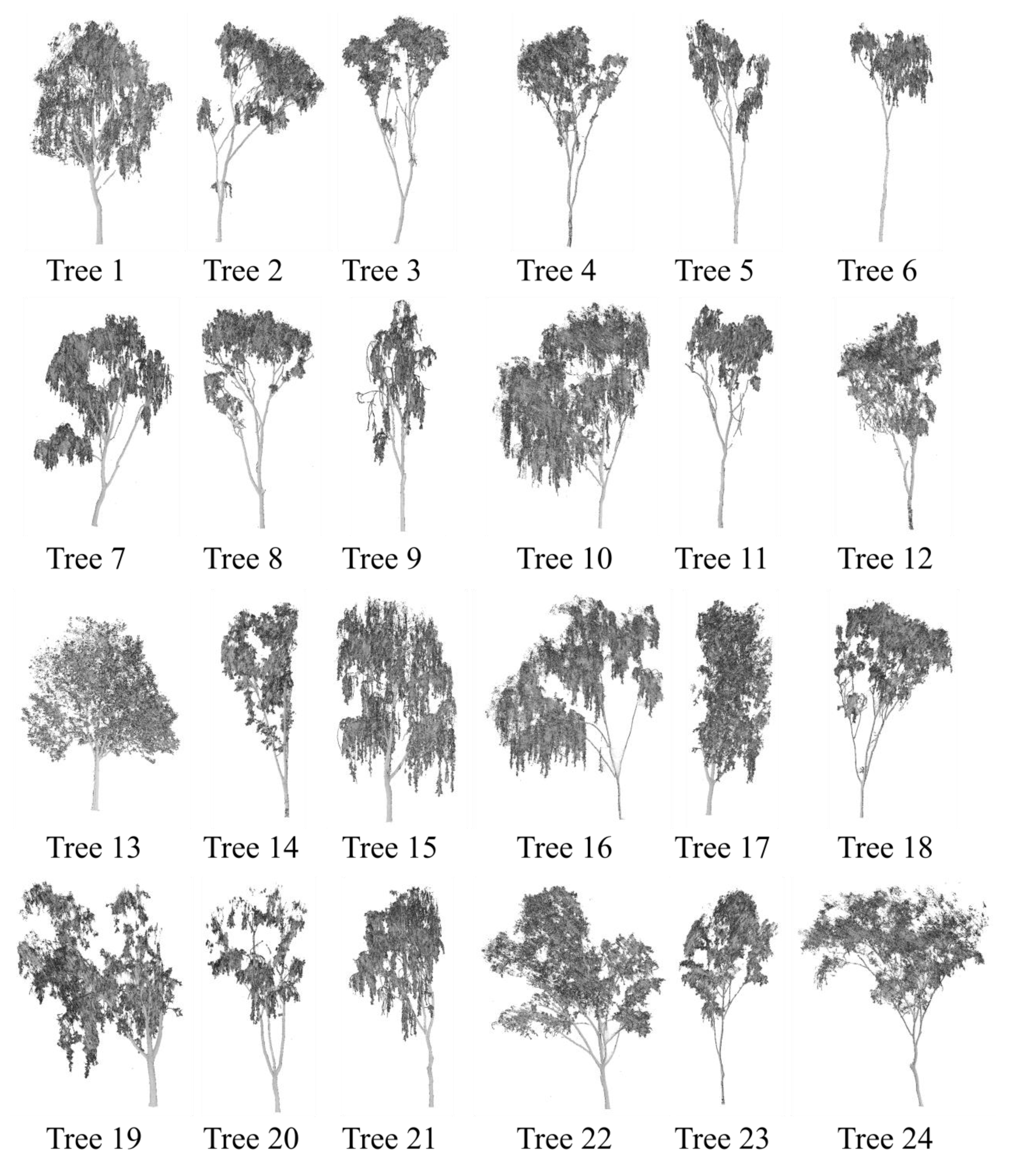
2.1. Experimental Data
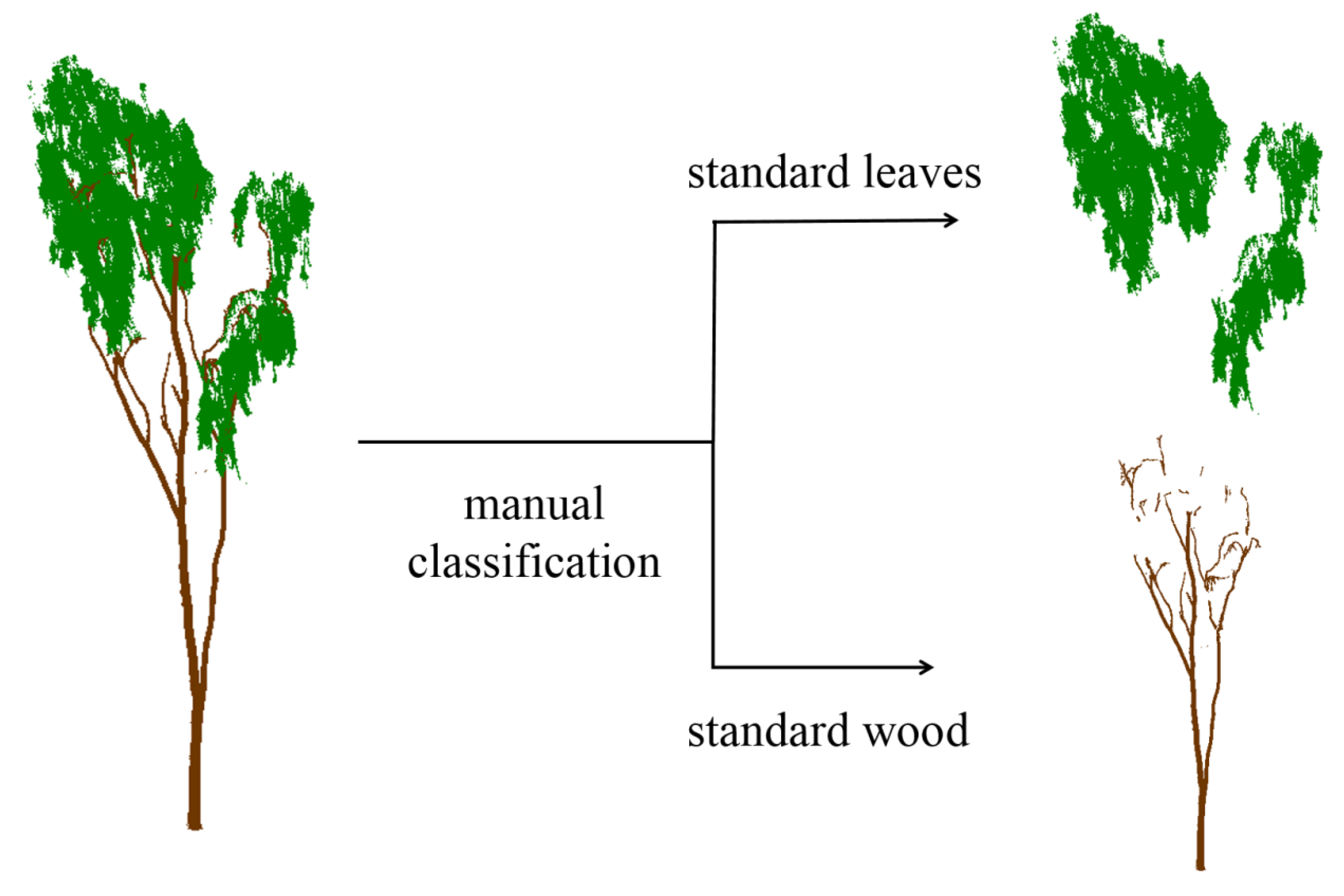
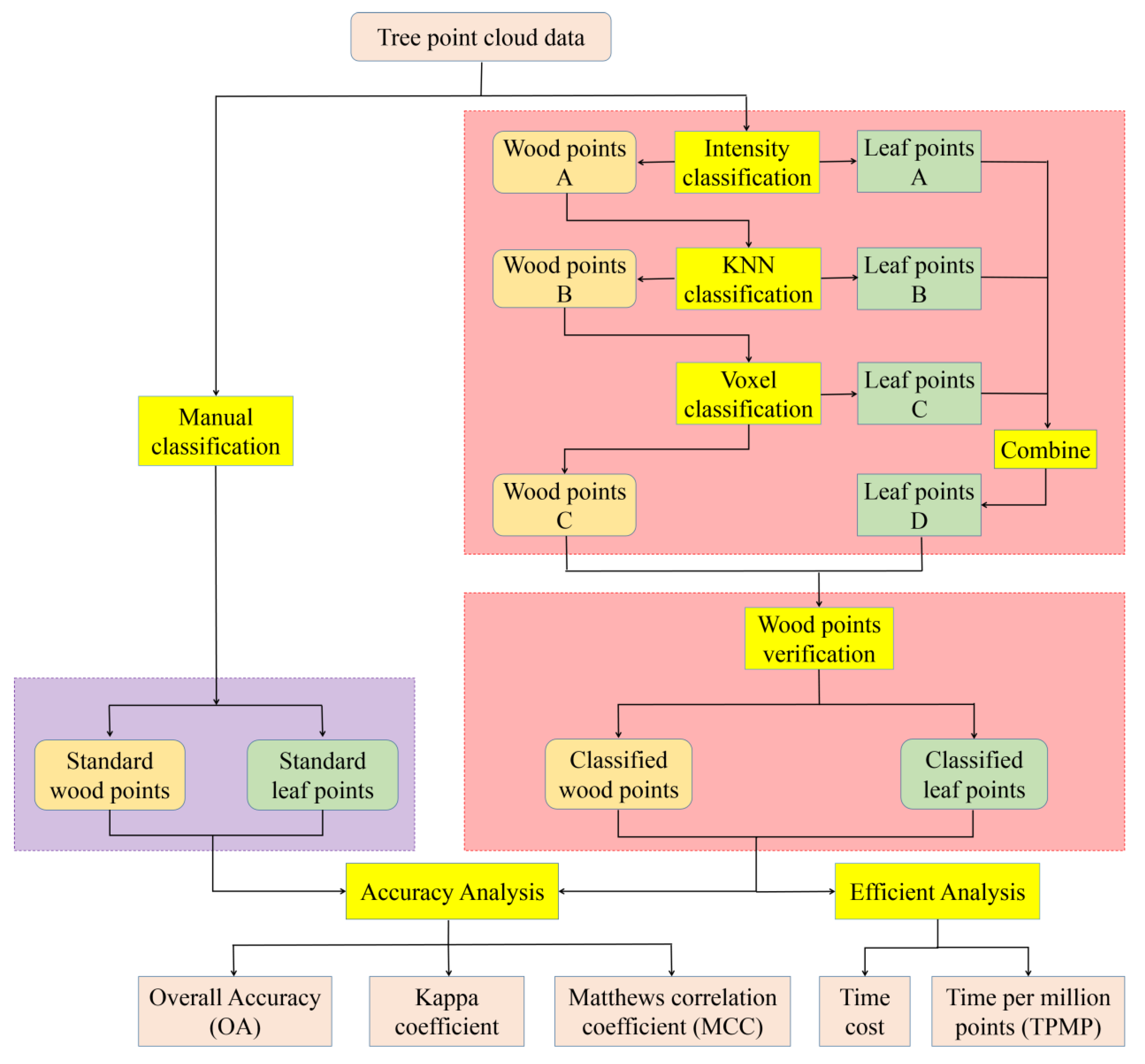
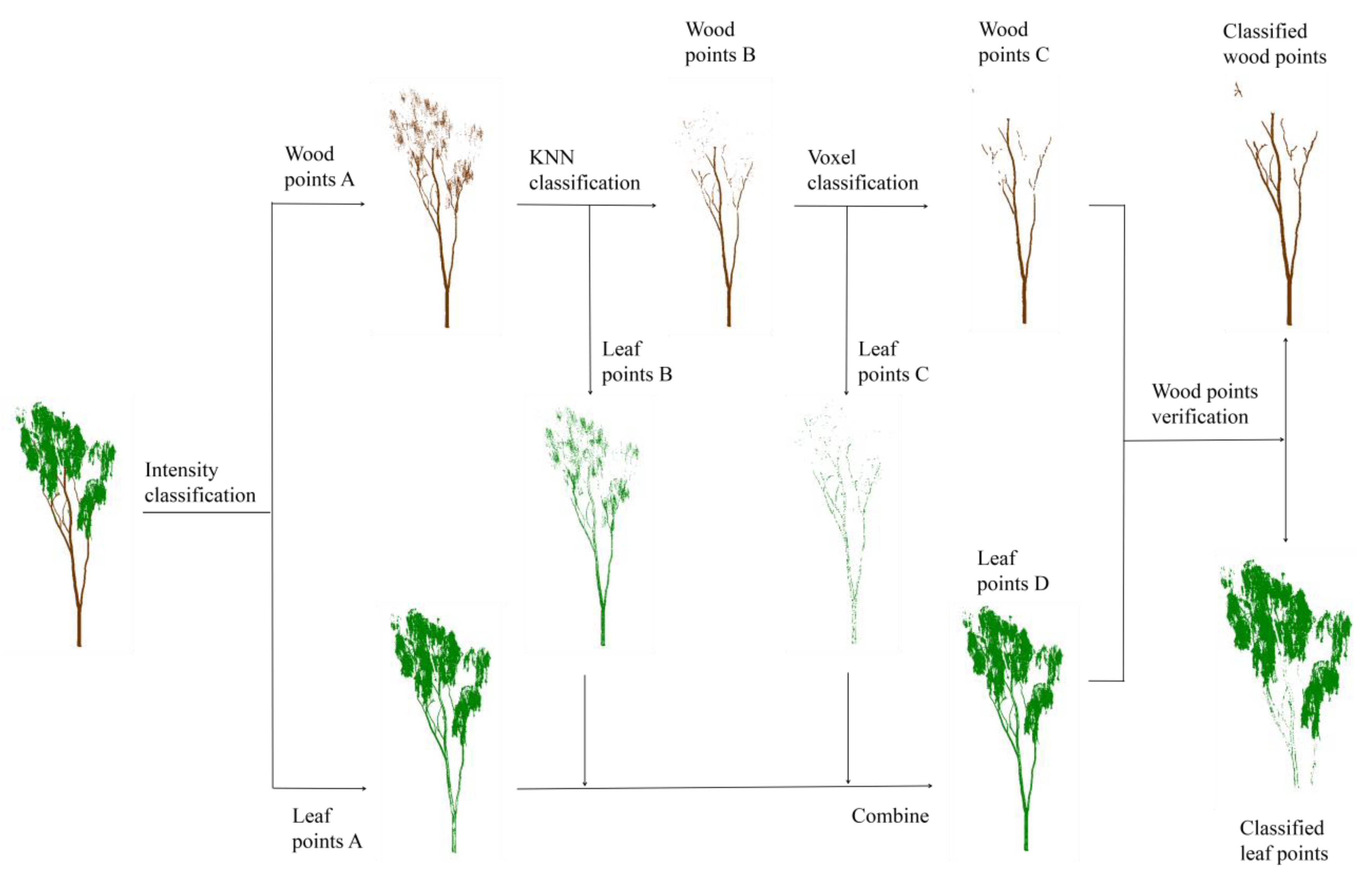
2.2. Method
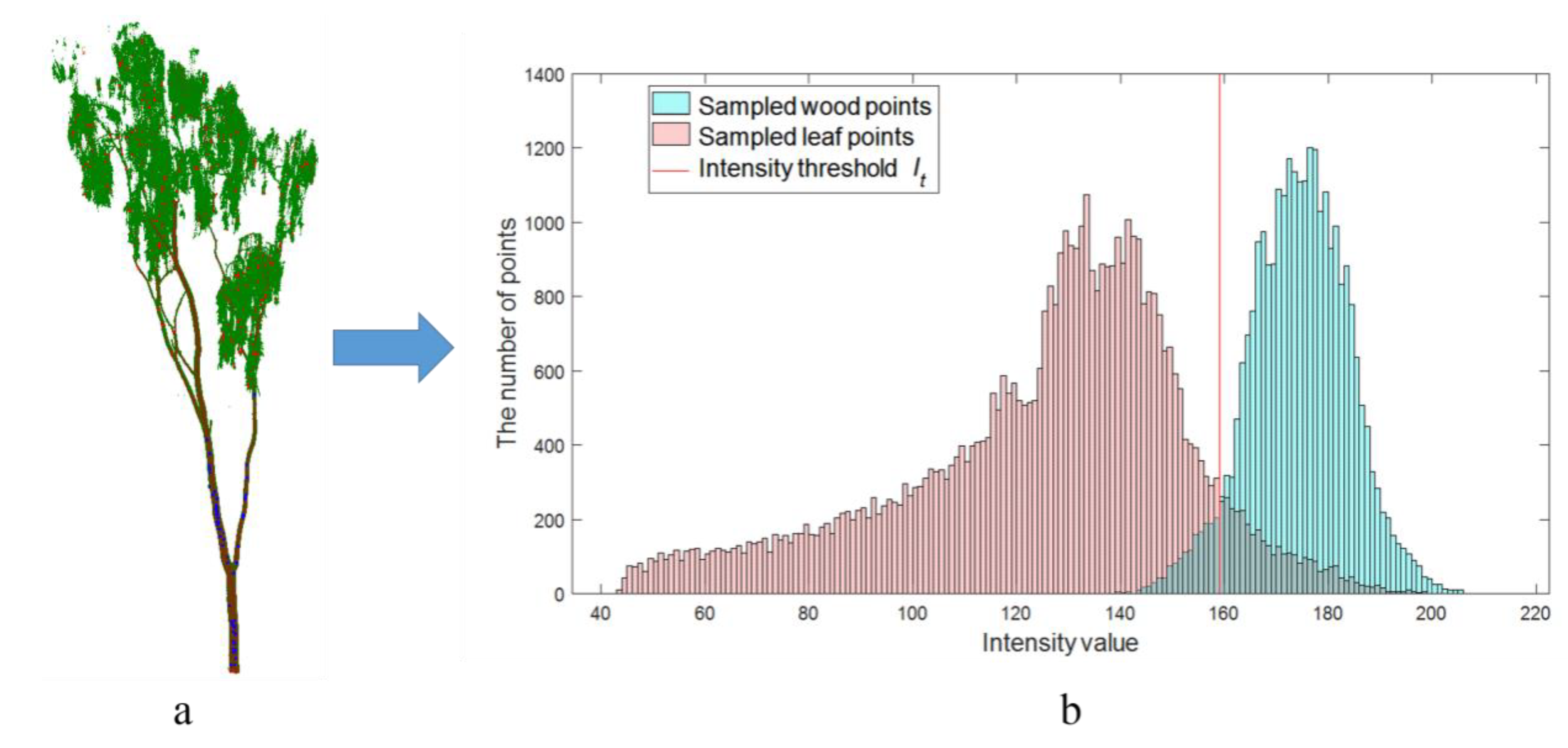
2.2.1. Intensity Classification
2.2.2. Neighborhood Classification
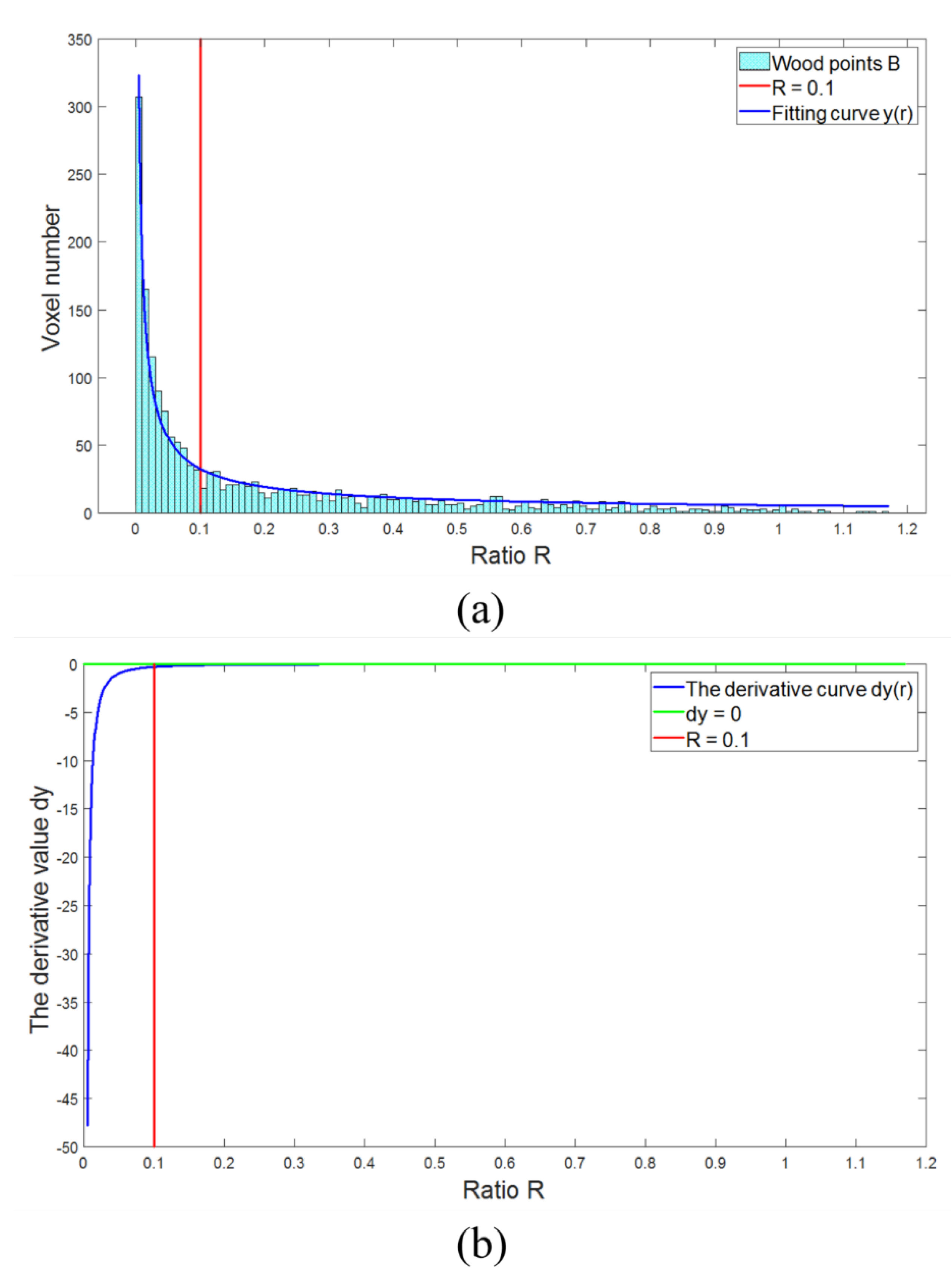
2.2.3. Voxel Classification
2.2.4. Wood Point Verification
- (1)
- The value of each wood point in the voxels was calculated according to Equation (2);
- (2)
- The distance between each wood point and leaf point in the voxels was calculated;
- (3)
- Then, the new wood point was determined according to the following formula:where is the intensity value of each leaf point. If a leaf point meets condition (a) or condition (b), the leaf point will be determined as a new wood point.
- (4)
- Check each leaf point in the neighbor voxels to complete the new wood point verification;
- (5)
- These new wood points were subjected to the above process until no more new wood points were found.
3. Results
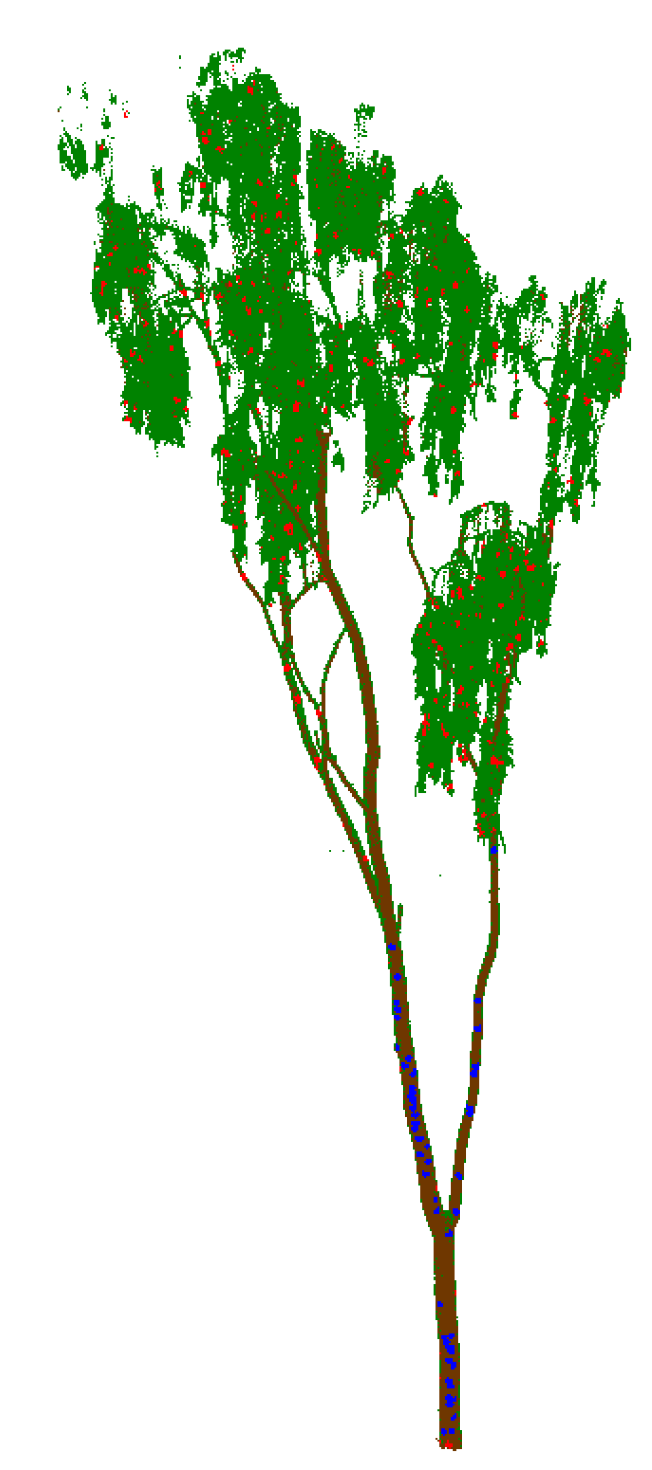
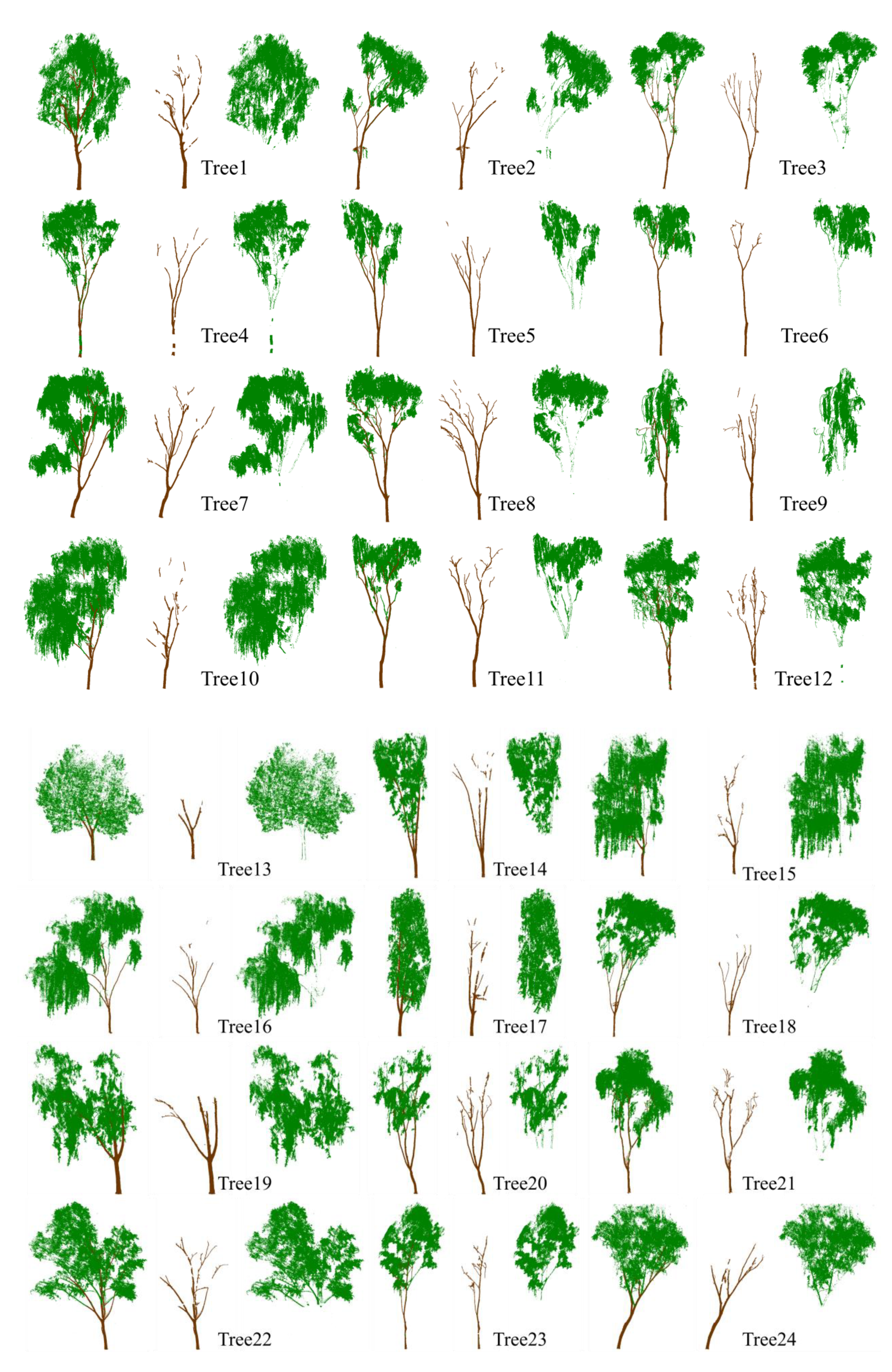
3.1. Classification Results
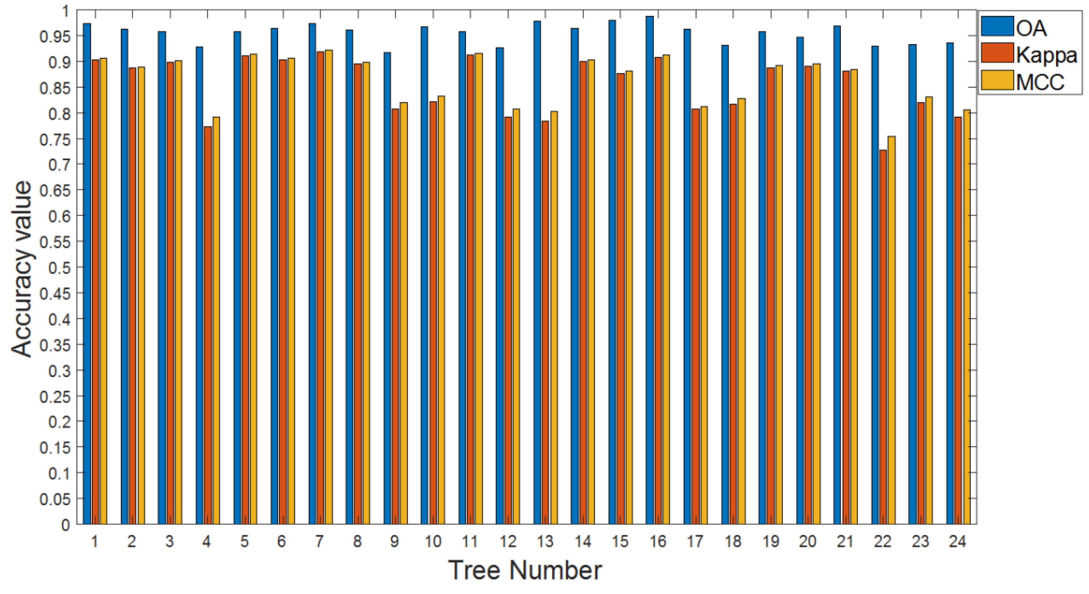
3.2. Accuracy and Efficiency Analysis
4. Discussion
5. Conclusions
Author Contributions
Funding
Data Availability Statement
Acknowledgments
Conflicts of Interest
References
- Lindenmayer, D.B.; Laurance, W.F.; Franklin, J.F.; Likens, G.E.; Banks, S.C.; Blanchard, W.; Gibbons, P.; Ikin, K.; Blair, D.; McBurney, L.; et al. New Policies for Old Trees: Averting a Global Crisis in a Keystone Ecological Structure: Rapid Loss of Large Old Trees. Conserv. Lett. 2014, 7, 61–69. [Google Scholar] [CrossRef]
- Food and Agriculture Organization of the United Nations. Global Forest Resources Assessment 2005: Progress towards Sustainable Forest Management; FAO forestry paper 147; Food and Agriculture Organization of the United Nations: Rome, Italy, 2006; ISBN 978-92-5-105481-9. [Google Scholar]
- Sohngen, B. An Analysis of Forestry Carbon Sequestration as a Response to Climate Change; Copenhagen Consensus Center: Frederiksberg, Denmark, 2009. [Google Scholar]
- Mizanur Rahman, M.; Nabiul Islam Khan, M.; Fazlul Hoque, A.K.; Ahmed, I. Carbon stock in the Sundarbans mangrove forest: Spatial variations in vegetation types and salinity zones. Wetl. Ecol. Manag. 2015, 23, 269–283. [Google Scholar] [CrossRef]
- Ross, M.S.; Ruiz, P.L.; Telesnicki, G.J.; Meeder, J.F. Estimating Above-Ground Biomass and Production in Mangrove Communities of Biscayne National Park, Florida (USA). Wetl. Ecol. Manag. 2001, 9, 27–37. [Google Scholar] [CrossRef]
- van Leeuwen, M.; Nieuwenhuis, M. Retrieval of Forest Structural Parameters Using LiDAR Remote Sensing. Eur. J. Forest Res. 2010, 129, 749–770. [Google Scholar] [CrossRef]
- Popescu, S.C. Estimating Biomass of Individual Pine Trees Using Airborne Lidar. Biomass Bioenergy 2007, 31, 646–655. [Google Scholar] [CrossRef]
- Lin, Y.; Herold, M. Tree Species Classification Based on Explicit Tree Structure Feature Parameters Derived from Static Terrestrial Laser Scanning Data. Agric. For. Meteorol. 2016, 216, 105–114. [Google Scholar] [CrossRef]
- Terryn, L.; Calders, K.; Disney, M.; Origo, N.; Malhi, Y.; Newnham, G.; Raumonen, P.; Å kerblom, M.; Verbeeck, H. Tree Species Classification Using Structural Features Derived from Terrestrial Laser Scanning. ISPRS J. Photogramm. Remote. Sens. 2020, 168, 170–181. [Google Scholar] [CrossRef]
- Calders, K.; Newnham, G.; Burt, A.; Murphy, S.; Raumonen, P.; Herold, M.; Culvenor, D.; Avitabile, V.; Disney, M.; Armston, J.; et al. Nondestructive Estimates of Above-ground Biomass Using Terrestrial Laser Scanning. Methods Ecol. Evol. 2015, 6, 198–208. [Google Scholar] [CrossRef]
- Means, J.E.; Acker, S.A.; Renslow, M.; Emerson, L.; Hendrix, C.J. Predicting Forest Stand Characteristics with Airborne Scanning Lidar. Photogramm. Eng. Remote Sens. 2000, 66, 1367–1372. [Google Scholar]
- Asner, G.P.; Powell, G.V.N.; Mascaro, J.; Knapp, D.E.; Clark, J.K.; Jacobson, J.; Kennedy-Bowdoin, T.; Balaji, A.; Paez-Acosta, G.; Victoria, E.; et al. High-Resolution Forest Carbon Stocks and Emissions in the Amazon. Proc. Natl. Acad. Sci. USA 2010, 107, 16738–16742. [Google Scholar] [CrossRef] [Green Version]
- Palace, M.; Sullivan, F.B.; Ducey, M.; Herrick, C. Estimating Tropical Forest Structure Using a Terrestrial Lidar. PLoS ONE 2016, 11, e0154115. [Google Scholar] [CrossRef] [PubMed]
- Hosoi, F.; Nakai, Y.; Omasa, K. Estimation and Error Analysis of Woody Canopy Leaf Area Density Profiles Using 3-D Airborne and Ground-Based Scanning Lidar Remote-Sensing Techniques. IEEE Trans. Geosci. Remote Sens. 2010, 48, 9. [Google Scholar] [CrossRef]
- Zheng, G.; Moskal, L.M.; Kim, S.-H. Retrieval of Effective Leaf Area Index in Heterogeneous Forests with Terrestrial Laser Scanning. IEEE Trans. Geosci. Remote Sens. 2013, 51, 777–786. [Google Scholar] [CrossRef]
- Olsoy, P.J.; Mitchell, J.J.; Levia, D.F.; Clark, P.E.; Glenn, N.F. Estimation of Big Sagebrush Leaf Area Index with Terrestrial Laser Scanning. Ecol. Indic. 2016, 61, 815–821. [Google Scholar] [CrossRef]
- Béland, M.; Widlowski, J.-L.; Fournier, R.A. A Model for Deriving Voxel-Level Tree Leaf Area Density Estimates from Ground-Based LiDAR. Environ. Model Softw. 2014, 51, 184–189. [Google Scholar] [CrossRef]
- Béland, M.; Baldocchi, D.D.; Widlowski, J.-L.; Fournier, R.A.; Verstraete, M.M. On Seeing the Wood from the Leaves and the Role of Voxel Size in Determining Leaf Area Distribution of Forests with Terrestrial LiDAR. Agric. For. Meteorol. 2014, 184, 82–97. [Google Scholar] [CrossRef]
- Kong, F.; Yan, W.; Zheng, G.; Yin, H.; Cavan, G.; Zhan, W.; Zhang, N.; Cheng, L. Retrieval of Three-Dimensional Tree Canopy and Shade Using Terrestrial Laser Scanning (TLS) Data to Analyze the Cooling Effect of Vegetation. Agric. For. Meteorol. 2016, 217, 22–34. [Google Scholar] [CrossRef]
- Xu, W.; Su, Z.; Feng, Z.; Xu, H.; Jiao, Y.; Yan, F. Comparison of Conventional Measurement and LiDAR-Based Measurement for Crown Structures. Comput. Electron. Agric. 2013, 98, 242–251. [Google Scholar] [CrossRef]
- Oveland, I.; Hauglin, M.; Gobakken, T.; Næsset, E.; Maalen-Johansen, I. Automatic Estimation of Tree Position and Stem Diameter Using a Moving Terrestrial Laser Scanner. Remote Sens. 2017, 9, 350. [Google Scholar] [CrossRef] [Green Version]
- Hauglin, M.; Astrup, R.; Gobakken, T.; Næsset, E. Estimating Single-Tree Branch Biomass of Norway Spruce with Terrestrial Laser Scanning Using Voxel-Based and Crown Dimension Features. Scand. J. For. Res. 2013, 28, 456–469. [Google Scholar] [CrossRef]
- Yu, X.; Liang, X.; Hyyppä, J.; Kankare, V.; Vastaranta, M.; Holopainen, M. Stem Biomass Estimation Based on Stem Reconstruction from Terrestrial Laser Scanning Point Clouds. Remote Sens. Lett. 2013, 4, 344–353. [Google Scholar] [CrossRef]
- McHale, M.R. Volume Estimates of Trees with Complex Architecture from Terrestrial Laser Scanning. J. Appl. Remote Sens. 2008, 2, 023521. [Google Scholar] [CrossRef]
- Saarinen, N.; Kankare, V.; Vastaranta, M.; Luoma, V.; Pyörälä, J.; Tanhuanpää, T.; Liang, X.; Kaartinen, H.; Kukko, A.; Jaakkola, A.; et al. Feasibility of Terrestrial Laser Scanning for Collecting Stem Volume Information from Single Trees. ISPRS J. Photogramm. Remote Sens. 2017, 123, 140–158. [Google Scholar] [CrossRef]
- Liang, X.; Kankare, V.; Yu, X.; Hyyppa, J.; Holopainen, M. Automated Stem Curve Measurement Using Terrestrial Laser Scanning. IEEE Trans. Geosci. Remote Sens. 2014, 52, 1739–1748. [Google Scholar] [CrossRef]
- Kelbe, D.; van Aardt, J.; Romanczyk, P.; van Leeuwen, M.; Cawse-Nicholson, K. Single-Scan Stem Reconstruction Using Low-Resolution Terrestrial Laser Scanner Data. IEEE J. Sel. Top. Appl. Earth Obs. Remote Sens. 2015, 8, 3414–3427. [Google Scholar] [CrossRef]
- Pueschel, P.; Newnham, G.; Hill, J. Retrieval of Gap Fraction and Effective Plant Area Index from Phase-Shift Terrestrial Laser Scans. Remote Sens. 2014, 6, 2601–2627. [Google Scholar] [CrossRef] [Green Version]
- Zheng, G.; Ma, L.; He, W.; Eitel, J.U.H.; Moskal, L.M.; Zhang, Z. Assessing the Contribution of Woody Materials to Forest Angular Gap Fraction and Effective Leaf Area Index Using Terrestrial Laser Scanning Data. IEEE Trans. Geosci. Remote Sens. 2016, 54, 1475–1487. [Google Scholar] [CrossRef]
- Ku, N.-W.; Popescu, S.C.; Ansley, R.J.; Perotto-Baldivieso, H.L.; Filippi, A.M. Assessment of Available Rangeland Woody Plant Biomass with a Terrestrial Lidar System. Photogramm. Eng. Remote Sens. 2012, 78, 349–361. [Google Scholar] [CrossRef]
- Kankare, V. Individual Tree Biomass Estimation Using Terrestrial Laser Scanning. ISPRS J. Photogramm. Remote Sens. 2013, 75, 64–75. [Google Scholar] [CrossRef]
- Béland, M.; Widlowski, J.-L.; Fournier, R.A.; Côté, J.-F.; Verstraete, M.M. Estimating Leaf Area Distribution in Savanna Trees from Terrestrial LiDAR Measurements. Agric. For. Meteorol. 2011, 151, 1252–1266. [Google Scholar] [CrossRef]
- Yao, T.; Yang, X.; Zhao, F.; Wang, Z.; Zhang, Q.; Jupp, D.; Lovell, J.; Culvenor, D.; Newnham, G.; Ni-Meister, W.; et al. Measuring Forest Structure and Biomass in New England Forest Stands Using Echidna Ground-Based Lidar. Remote Sens. Environ. 2011, 115, 2965–2974. [Google Scholar] [CrossRef]
- Yang, X.; Strahler, A.H.; Schaaf, C.B.; Jupp, D.L.B.; Yao, T.; Zhao, F.; Wang, Z.; Culvenor, D.S.; Newnham, G.J.; Lovell, J.L.; et al. Three-Dimensional Forest Reconstruction and Structural Parameter Retrievals Using a Terrestrial Full-Waveform Lidar Instrument (Echidna ®). Remote Sens. Environ. 2013, 135, 36–51. [Google Scholar] [CrossRef]
- Douglas, E.S.; Martel, J.; Li, Z.; Howe, G.; Hewawasam, K.; Marshall, R.A.; Schaaf, C.L.; Cook, T.A.; Newnham, G.J.; Strahler, A.; et al. Finding Leaves in the Forest: The Dual-Wavelength Echidna Lidar. IEEE Geosci. Remote Sens. Lett. 2015, 12, 776–780. [Google Scholar] [CrossRef]
- Zhao, X.; Shi, S.; Yang, J.; Gong, W.; Sun, J.; Chen, B.; Guo, K.; Chen, B. Active 3D Imaging of Vegetation Based on Multi-Wavelength Fluorescence LiDAR. Sensors 2020, 20, 935. [Google Scholar] [CrossRef] [Green Version]
- Tao, S.; Guo, Q.; Xu, S.; Su, Y.; Li, Y.; Wu, F. A Geometric Method for Wood-Leaf Separation Using Terrestrial and Simulated Lidar Data. Photogram. Eng. Rem. Sens. 2015, 81, 767–776. [Google Scholar] [CrossRef]
- Ma, L.; Zheng, G.; Eitel, J.U.H.; Moskal, L.M.; He, W.; Huang, H. Improved Salient Feature-Based Approach for Automatically Separating Photosynthetic and Nonphotosynthetic Components Within Terrestrial Lidar Point Cloud Data of Forest Canopies. IEEE Trans. Geosci. Remote Sens. 2016, 54, 679–696. [Google Scholar] [CrossRef]
- Ferrara, R.; Virdis, S.G.P.; Ventura, A.; Ghisu, T.; Duce, P.; Pellizzaro, G. An Automated Approach for Wood-Leaf Separation from Terrestrial LIDAR Point Clouds Using the Density Based Clustering Algorithm DBSCAN. Agric. For. Meteorol. 2018, 262, 434–444. [Google Scholar] [CrossRef]
- Xiang, L.; Bao, Y.; Tang, L.; Ortiz, D.; Salas-Fernandez, M.G. Automated Morphological Traits Extraction for Sorghum Plants via 3D Point Cloud Data Analysis. Comput. Electron. Agric. 2019, 162, 951–961. [Google Scholar] [CrossRef]
- Wang, D.; Momo Takoudjou, S.; Casella, E. LeWoS: A Universal Leaf-wood Classification Method to Facilitate the 3D Modelling of Large Tropical Trees Using Terrestrial LiDAR. Methods Ecol. Evol. 2020, 11, 376–389. [Google Scholar] [CrossRef]
- Yun, T.; An, F.; Li, W.; Sun, Y.; Cao, L.; Xue, L. A Novel Approach for Retrieving Tree Leaf Area from Ground-Based LiDAR. Remote Sens. 2016, 8, 942. [Google Scholar] [CrossRef] [Green Version]
- Zhu, X.; Skidmore, A.K.; Darvishzadeh, R.; Niemann, K.O.; Liu, J.; Shi, Y.; Wang, T. Foliar and Woody Materials Discriminated Using Terrestrial LiDAR in a Mixed Natural Forest. Int. J. Appl. Earth Obs. Geoinf. 2018, 64, 43–50. [Google Scholar] [CrossRef]
- Vicari, M.B.; Disney, M.; Wilkes, P.; Burt, A.; Calders, K.; Woodgate, W. Leaf and Wood Classification Framework for Terrestrial LiDAR Point Clouds. Methods Ecol. Evol. 2019, 10, 680–694. [Google Scholar] [CrossRef] [Green Version]
- Liu, Z.; Zhang, Q.; Wang, P.; Li, Z.; Wang, H. Automated Classification of Stems and Leaves of Potted Plants Based on Point Cloud Data. Biosyst. Eng. 2020, 200, 215–230. [Google Scholar] [CrossRef]
- Liu, Z.; Zhang, Q.; Wang, P.; Li, Y.; Sun, J. Automatic Sampling and Training Method for Wood-Leaf Classification Based on Tree Terrestrial Point Cloud. arXiv 2020, arXiv:2012.03152 [cs]. [Google Scholar]
- Krishna Moorthy, S.M.; Calders, K.; Vicari, M.B.; Verbeeck, H. Improved Supervised Learning-Based Approach for Leaf and Wood Classification from LiDAR Point Clouds of Forests. IEEE Trans. Geosci. Remote Sens. 2020, 58, 3057–3070. [Google Scholar] [CrossRef] [Green Version]
- Morel, J.; Bac, A.; Kanai, T. Segmentation of Unbalanced and In-Homogeneous Point Clouds and Its Application to 3D Scanned Trees. Vis. Comput. 2020, 36, 2419–2431. [Google Scholar] [CrossRef]
- Soudarissanane, S.; Lindenbergh, R.; Menenti, M.; Teunissen, P. Scanning Geometry: Influencing Factor on the Quality of Terrestrial Laser Scanning Points. ISPRS J. Photogramm. Remote Sens. 2011, 66, 389–399. [Google Scholar] [CrossRef]
- Matthews, B.W. Comparison of the Predicted and Observed Secondary Structure of T4 Phage Lysozyme. Biochim. Biophys. Acta (BBA) -Protein Struct. 1975, 405, 442–451. [Google Scholar] [CrossRef]
- Delgado, R.; Tibau, X.-A. Why Cohen’s Kappa Should Be Avoided as Performance Measure in Classification. PLoS ONE 2019, 14, e0222916. [Google Scholar] [CrossRef] [Green Version]
- Pfeifer, N.; Gorte, B.; Winterhalder, D. Automatic reconstruction of single trees from terrestrial laser scanner data. In Proceedings of the 20th ISPRS Congress, Istanbul, Turkey, 12–23 July 2004; Volume 35, pp. 114–119. [Google Scholar]


| Technical Parameters | |
|---|---|
| The farthest distance measurement | 600 m (Natural object reflectivity ≥ 90%) |
| The scanning rate (points/second) | 300000 (emission), 125000 (reception) |
| The vertical scanning range | −40°–60° |
| The horizontal scanning range | 0°–360° |
| Laser divergence | 0.3 mrad |
| The scanning accuracy | 3 mm (single measurement), 2 mm (multiple measurements) |
| The angular resolution | Better than 0.0005° (in both vertical and horizontal directions) |
| Tree/Number | Total Points | TTH (m) | DBH (m) | Distance (m) |
|---|---|---|---|---|
| 1 | 876657 | 13.90 | 0.29 | 14.63 |
| 2 | 716701 | 13.33 | 0.20 | 10.26 |
| 3 | 629250 | 13.75 | 0.24 | 12.26 |
| 4 | 733233 | 15.12 | 0.26 | 13.03 |
| 5 | 1064546 | 13.08 | 0.18 | 6.07 |
| 6 | 971915 | 11.88 | 0.15 | 6.56 |
| 7 | 3398859 | 13.30 | 0.26 | 6.39 |
| 8 | 1162123 | 13.61 | 0.23 | 10.86 |
| 9 | 1068644 | 9.87 | 0.14 | 5.21 |
| 10 | 1210685 | 14.40 | 0.29 | 15.23 |
| 11 | 1318700 | 13.96 | 0.26 | 5.93 |
| 12 | 742280 | 14.87 | 0.27 | 14.22 |
| 13 | 203303 | 10.02 | 0.26 | 36.99 |
| 14 | 1896619 | 13.71 | 0.25 | 6.83 |
| 15 | 1080397 | 13.27 | 0.28 | 14.85 |
| 16 | 980776 | 12.41 | 0.20 | 14.25 |
| 17 | 841575 | 15.18 | 0.28 | 17.11 |
| 18 | 1357196 | 13.33 | 0.21 | 7.06 |
| 19 | 4925230 | 8.82 | 0.28 | 3.74 |
| 20 | 1716488 | 14.30 | 0.25 | 5.94 |
| 21 | 1275620 | 13.63 | 0.21 | 11.45 |
| 22 | 1301100 | 11.73 | 0.24 | 10.68 |
| 23 | 1315914 | 14.65 | 0.23 | 7.69 |
| 24 | 771395 | 11.05 | 0.23 | 11.45 |
| Intensity Classification | KNN Classification | Voxel Classification | Combine | Wood Point Verification |
|---|---|---|---|---|
| wood points A | wood points B | wood points C | / | classified wood points |
| 301392 | 261408 | 242513 | / | 393211 |
| leaf points A | leaf points B | leaf points C | leaf points D | classified leaf points |
| 763154 | 39984 | 18895 | 822033 | 671335 |
| Tree/Number | Total Points | Standard Results | Classification Results | ||||
|---|---|---|---|---|---|---|---|
| Wood Points | Leaf Points | Wood Points | Leaf Points | ||||
| True | False | True | False | ||||
| 1 | 876657 | 150479 | 726178 | 128879 | 1215 | 724963 | 21600 |
| 2 | 716701 | 154548 | 562153 | 133791 | 5647 | 556506 | 20757 |
| 3 | 629250 | 190793 | 438457 | 166616 | 2080 | 436377 | 24177 |
| 4 | 733233 | 169071 | 564162 | 116880 | 651 | 563511 | 52191 |
| 5 | 1064546 | 427139 | 637407 | 384086 | 1592 | 635815 | 43053 |
| 6 | 971915 | 246251 | 725664 | 213843 | 1899 | 723765 | 32408 |
| 7 | 3398859 | 719573 | 2679286 | 638655 | 7436 | 2671850 | 80918 |
| 8 | 1162123 | 312819 | 849304 | 271612 | 4924 | 844380 | 41207 |
| 9 | 1068644 | 374865 | 693779 | 289835 | 3926 | 689853 | 85030 |
| 10 | 1210685 | 143532 | 1067153 | 105130 | 1653 | 1065500 | 38402 |
| 11 | 1318700 | 562884 | 755816 | 508514 | 1065 | 754751 | 54370 |
| 12 | 742280 | 193707 | 548573 | 140832 | 1491 | 547082 | 52875 |
| 13 | 203303 | 13301 | 190002 | 8801 | 37 | 189965 | 4500 |
| 14 | 1896619 | 482532 | 1414087 | 420063 | 7086 | 1407001 | 62469 |
| 15 | 1080397 | 109269 | 971128 | 88755 | 1962 | 969166 | 20514 |
| 16 | 980776 | 79224 | 901552 | 66944 | 184 | 901368 | 12280 |
| 17 | 841575 | 100118 | 741457 | 76668 | 8182 | 733275 | 23450 |
| 18 | 1357196 | 375669 | 981527 | 286918 | 4034 | 977493 | 88751 |
| 19 | 4925230 | 1329062 | 3596168 | 1128847 | 8731 | 3587437 | 200215 |
| 20 | 1716488 | 727900 | 988588 | 644566 | 6718 | 981870 | 83334 |
| 21 | 1275620 | 215761 | 1059859 | 179962 | 4550 | 1055309 | 35799 |
| 22 | 1301100 | 240684 | 1060416 | 150458 | 1391 | 1059025 | 90226 |
| 23 | 1315914 | 364161 | 951753 | 279447 | 3560 | 948193 | 84714 |
| 24 | 771395 | 165762 | 605623 | 118643 | 1805 | 603828 | 47119 |
| Tree/Number | Accuracy Analysis | Time Analysis | |||
|---|---|---|---|---|---|
| OA | Kappa | MCC | Time Cost (ms) | TPMP (ms) | |
| 1 | 0.9739 | 0.9032 | 0.9066 | 935 | 1067 |
| 2 | 0.9631 | 0.8870 | 0.8889 | 930 | 1298 |
| 3 | 0.9582 | 0.8979 | 0.9012 | 870 | 1383 |
| 4 | 0.9279 | 0.7726 | 0.7923 | 912 | 1244 |
| 5 | 0.9580 | 0.9113 | 0.9144 | 1901 | 1786 |
| 6 | 0.9647 | 0.9027 | 0.9061 | 1350 | 1390 |
| 7 | 0.9740 | 0.9191 | 0.9211 | 5547 | 1633 |
| 8 | 0.9603 | 0.8952 | 0.8983 | 1565 | 1347 |
| 9 | 0.9167 | 0.8076 | 0.8203 | 1625 | 1521 |
| 10 | 0.9669 | 0.8219 | 0.8331 | 1103 | 912 |
| 11 | 0.9579 | 0.9130 | 0.9162 | 2456 | 1863 |
| 12 | 0.9267 | 0.7923 | 0.8080 | 917 | 1236 |
| 13 | 0.9776 | 0.7837 | 0.8021 | 506 | 2489 |
| 14 | 0.9633 | 0.8995 | 0.9024 | 2981 | 1572 |
| 15 | 0.9792 | 0.8762 | 0.8808 | 990 | 917 |
| 16 | 0.9872 | 0.9080 | 0.9116 | 880 | 898 |
| 17 | 0.9624 | 0.8080 | 0.8115 | 791 | 940 |
| 18 | 0.9316 | 0.8164 | 0.8281 | 1789 | 1319 |
| 19 | 0.9575 | 0.8872 | 0.8919 | 12753 | 2590 |
| 20 | 0.9475 | 0.8910 | 0.8949 | 3517 | 2049 |
| 21 | 0.9683 | 0.8805 | 0.8843 | 1334 | 1046 |
| 22 | 0.9295 | 0.7276 | 0.7544 | 1392 | 1070 |
| 23 | 0.9329 | 0.8200 | 0.8315 | 1778 | 1352 |
| 24 | 0.9365 | 0.7913 | 0.8065 | 938 | 1216 |
| Mean | 0.9550 | 0.8547 | 0.8627 | / | 1423 |
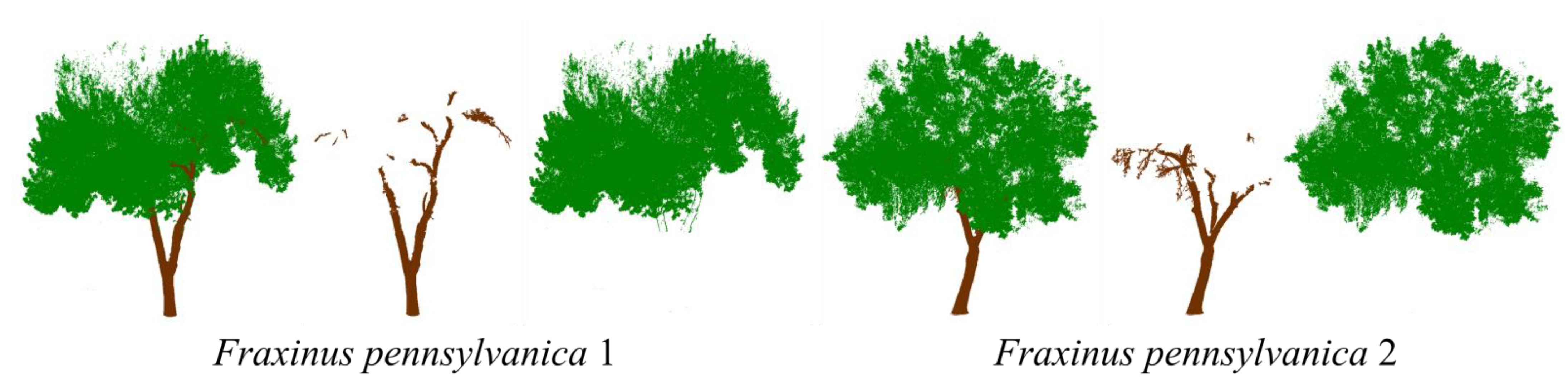
| Tree/Number | Total Points | Standard Results | Classification Results | ||||
|---|---|---|---|---|---|---|---|
| Wood Points | Leaf Points | Wood Points | Leaf Points | ||||
| True | False | True | False | ||||
| Fraxinus pennsylvanica 1 | 3523822 | 350208 | 3173614 | 225688 | 8344 | 3165270 | 124520 |
| Fraxinus pennsylvanica 1 | 2164520 | 182081 | 1982439 | 146612 | 3661 | 1978778 | 35469 |
| Tree/Number | Accuracy Analysis | Time Analysis | |||
|---|---|---|---|---|---|
| OA | Kappa | MCC | Time Cost (ms) | TPMP (ms) | |
| Fraxinus pennsylvanica 1 | 0.9622 | 0.7529 | 0.7711 | 3369 | 957 |
| Fraxinus pennsylvanica 2 | 0.9819 | 0.8725 | 0.8772 | 2200 | 1017 |
Publisher’s Note: MDPI stays neutral with regard to jurisdictional claims in published maps and institutional affiliations. |
© 2021 by the authors. Licensee MDPI, Basel, Switzerland. This article is an open access article distributed under the terms and conditions of the Creative Commons Attribution (CC BY) license (https://creativecommons.org/licenses/by/4.0/).
Share and Cite
Sun, J.; Wang, P.; Gao, Z.; Liu, Z.; Li, Y.; Gan, X.; Liu, Z. Wood–Leaf Classification of Tree Point Cloud Based on Intensity and Geometric Information. Remote Sens. 2021, 13, 4050. https://doi.org/10.3390/rs13204050
Sun J, Wang P, Gao Z, Liu Z, Li Y, Gan X, Liu Z. Wood–Leaf Classification of Tree Point Cloud Based on Intensity and Geometric Information. Remote Sensing. 2021; 13(20):4050. https://doi.org/10.3390/rs13204050
Chicago/Turabian StyleSun, Jingqian, Pei Wang, Zhiyong Gao, Zichu Liu, Yaxin Li, Xiaozheng Gan, and Zhongnan Liu. 2021. "Wood–Leaf Classification of Tree Point Cloud Based on Intensity and Geometric Information" Remote Sensing 13, no. 20: 4050. https://doi.org/10.3390/rs13204050
APA StyleSun, J., Wang, P., Gao, Z., Liu, Z., Li, Y., Gan, X., & Liu, Z. (2021). Wood–Leaf Classification of Tree Point Cloud Based on Intensity and Geometric Information. Remote Sensing, 13(20), 4050. https://doi.org/10.3390/rs13204050