Article

Estimation of Plot-Level Burn Severity Using Terrestrial Laser Scanning

by
Michael R. Gallagher
1,*,
Aaron E. Maxwell
2,
Luis Andrés Guillén
3,
Alexis Everland
4,
E. Louise Loudermilk
5 and
Nicholas S. Skowronski
6
1
USDA Forest Service, Northern Research Station, New Lisbon, NJ 08064, USA
2
Department of Geology and Geography, West Virginia University, Morgantown, WV 26506, USA
3
Southern Swedish Forest Research Centre, Swedish University of Agricultural Science, P.O. Box 49, SE-230 53 Alnarp, Sweden
4
USDA Forest Service, Southern Research Station, Athens Fire Laboratory, 320 Green Street, Athens, GA 30602, USA
5
New Jersey Department of Environmental Protection, Forest Fire Service, P.O. Box 239, New Lisbon, NJ 08064, USA
6
USDA Forest Service, Northern Research Station, Morgantown, WV 26506, USA
*
Author to whom correspondence should be addressed.
Remote Sens. 2021, 13(20), 4168; https://doi.org/10.3390/rs13204168
Submission received: 9 September 2021 / Revised: 2 October 2021 / Accepted: 12 October 2021 / Published: 18 October 2021
(This article belongs to the Special Issue Advances in LiDAR Remote Sensing for Forestry and Ecology)

Abstract

:
Monitoring wildland fire burn severity is important for assessing ecological outcomes of fire and their spatial patterning as well as guiding efforts to mitigate or restore areas where ecological outcomes are negative. Burn severity mapping products are typically created using satellite reflectance data but must be calibrated to field data to derive meaning. The composite burn index (CBI) is the most widely used field-based method used to calibrate satellite-based burn severity data but important limitations of this approach have yet to be resolved. The objective of this study was focused on predicting CBI from point cloud and visible-spectrum camera (RGB) metrics derived from single-scan terrestrial laser scanning (TLS) datasets to determine the viability of TLS data as an alternative approach to estimating burn severity in the field. In our approach, we considered the predictive potential of post-scan-only metrics, differenced pre- and post-scan metrics, RGB metrics, and all three together to predict CBI and evaluated these with candidate algorithms (i.e., linear model, random forest (RF), and support vector machines (SVM) and two evaluation criteria (R-squared and root mean square error (RMSE)). In congruence with the strata-based observations used to calculate CBI, we evaluated the potential approaches at the strata level and at the plot level using 70 TLS and 10 RGB independent variables that we generated from the field data. Machine learning algorithms successfully predicted total plot CBI and strata-specific CBI; however, the accuracy of predictions varied among strata by algorithm. RGB variables improved predictions when used in conjunction with TLS variables, but alone proved a poor predictor of burn severity below the canopy. Although our study was to predict CBI, our results highlight that TLS-based methods for quantifying burn severity can be an improvement over CBI in many ways because TLS is repeatable, quantitative, faster, requires less field-expertise, and is more flexible to phenological variation and biomass change in the understory where prescribed fire effects are most pronounced. We also point out that TLS data can also be leveraged to inform other monitoring needs beyond those specific to wildland fire, representing additional efficiency in using this approach.

Graphical Abstract

1. Introduction

Wildland fires have varying effects on ecosystems that result from a complicated interplay between the pre-fire characteristics of the ecosystem such as species composition, three-dimensional structure, and topography [1], environmental conditions such as weather and drought status, and the dynamics of the fire (heat release, residence time, etc. [2]). Wildland fire managers aim to monitor fire effects both spatially and temporally to quantify the effectiveness of fuel reduction fire treatments, identify wildfire consequences, guide responsive post-fire management, justify fuels management needs, and better understand the ecological roles, patterns, and processes of wildland fire. There is a growing need to increase the pace and scale of fire effects monitoring in the management community particularly as prescribed fire programs and wildfire response expand to meet the growing challenges of fire suppression and ecosystem management.
Because monitoring fire effects directly is often intensive and tedious, there is substantial interest in developing and applying simpler and more efficient observation approaches from which fire effects can be inferred. The term “burn severity” is often used to describe some measure of a fire’s effect on an ecosystem, but there are varying arguments about its precise meaning [3,4,5]. Bond and Keeley [6] conceptualized “fire severity” as the loss of or change in organic matter aboveground and belowground while Simard [3] defined burn severity as the magnitude of significant negative fire impacts on wildland systems. Lastly, Hardy et al. [7] defined it as the intensity of the fire as it affects the biogeochemical environment. Overall, burn severity is important for identifying and monitoring fire impacts, which vary across landscapes and throughout the vertical structure of forests [8], and guides mitigation or restoration responses to ecologically negative consequences of fire [9]. However, this abstract term has led to subjective, inconsistent, and often indirect measurement techniques that need improvement to be considered rigorous and comparable.
Burn severity is often estimated as an index of surface reflectance estimated from remotely sensed near-infrared (NIR) and shortwave infrared (SWIR) data that are collected pre- and post-burn then differenced to calculate the change detection index known as the differenced normalized burn ratio (dNBR [10,11]). Unburned forests are characterized by higher NIR reflectance in comparison to SWIR while burned areas tend to show higher SWIR reflectance in comparison to NIR, a signature of bare soil as opposed to photosynthetically active vegetation [12]. Ignoring the impact of cloud cover, dNBR provides wall-to-wall coverage as a two-dimensional map of burn severity that can be extremely useful, although it is important to consider that organic matter loss from fire is only indirectly measured from spectral reflectance, and canopy cover can easily obscure lower-level changes in vegetation [13]. Without field reference data, two-dimensional remotely sensed burn severity products such as dNBR offer limited insight and dimensionality to fire effects on vegetation density and structure beneath the canopy [14], where effects are often targeted [15].
To bridge the gap between two-dimensional remote sensing burn severity products and understory and midstory effects of interest, the ‘composite burn index’ (CBI [11]) has been employed as the field-based standard reference despite important repeatability and subjectivity issues with the method [14,16,17]. CBI is generated at the plot level from visual assessments of fire effects, either in as effects (i.e., first-order effects) or as a long-term assessment that includes both fire-induced and other post-fire effects (i.e., second-order effects), in five forest strata: substrates (e.g., soil/rock and detritus), low shrubs and herbs (e.g., vegetation <1 m tall), tall shrubs and herbs (e.g., vegetation 1–5 m tall), pole size trees, and tall trees [11]. However, data are subjective relative to interpretation and assumptions of unmeasured pre-fire conditions by observers and may be biased toward specific strata due to prior management or forest growth form [14]. For instance, observers using this method visually “guess” percentages of fuel consumption, greenness, necrosis, and char following burning, without physical measurements or prior data as to fuel load, structure, or vegetation conditions which are instead inferred based on vegetation remaining post-fire and visual cues [11]. These qualitative estimates, which are subject to observer bias, are then used to index signatures of reflectance; however, similar spectral signatures may inadvertently lead to a grouping of characteristics that are dissimilar results of a fire. For instance, a low severity signature in satellite spectral data could hypothetically result either where understory severity was actually high but mostly obscured by dense undamaged canopy foliage, or where understory and overstory severity were actually homogenously low. The crux of this difference is the fact that fire effects are correlated inconsistently between forest strata [8].
Alternatively, airborne light detection and ranging (lidar; ALS) has been used to decompose the two-dimensional dNBR to three-dimensional effects on forest structure and density and to link pre-fire structure with resultant burn severity [8,18]. However, ALS typically has a much lower return density (per m2) than terrestrial laser scanning (TLS) collections (typically 2–5 pts. per m2 vs. 10–20 pts. per m2) and, as a result, does not provide detailed information about forest structure in lower forest strata where low to moderate severity fire effects are most prominent. Lower forest strata are most relevant for low-intensity surface fire regimes [14]. Further, ALS datasets are expensive to collect at temporal frequencies necessary to effectively monitor prescribed fire or wildfire effects consistently every year.
TLS excels in collecting structure and density data in understory and midstory strata where ALS is weakest due to canopy occlusion and can be conducted quickly with minimal training and no expertise in remote sensing or fire effects and thus offers a potential alternative to CBI as a consistent, repeatable, field-based approach to creating rich three-dimensional plot-level datasets of vegetation structure and density [19,20]. Kato et al. [20] used linear and non-linear regression to compare dNBR data with voxelized TLS data from burned plots and found that correlations were strongest when using all data (R2 = 0.73–0.75) but became weaker when data were binned according to CBI correlations with dNBR (R2 = 0.05–0.63). Alternatively, the Phillip and Levick [21] used linear regression to compare a new burn severity metric derived from Sentinel 2 C-band Synthetic Aperture Radar data with binned TLS point data and found consistent yet weak correlations (R2 = 0.23–0.37). However, to the best of our knowledge, no study has directly attempted to predict CBI from TLS derived metrics or has leveraged the full potential of information-rich TLS point-clouds with more sophisticated prediction approaches like machine learning algorithms to predict burn severity. Due to the benefits of TLS, predicting CBI can be an important step toward improving field estimation of burn severity in a way that can harmonize with existing monitoring programs, and predictions from which are likely to be improved with the use of machine learning.
Beyond the potential to predict burn severity, TLS also offers the complimentary benefit of also being a forest vegetation inventorying approach and can produce data that is richer and more dynamic for ecological analyses uses than CBI. TLS data have been used to estimate canopy characteristics outside of fire applications such as leaf area index [22], biomass [23,24], and canopy cover [25,26]. TLS collections have also targeted the mapping and measuring of individual trees [27,28]. More recently, TLS has been used to map fuels in three dimensions [29] and changes in forest structure following wildfire [30]. Additionally, because some TLS systems collect spectral reflectance data that are appended to each return, there is potential to integrate a spectral-reflectance index with the three-dimensional data for consistent fine-scale burn severity mapping [19,31]. With costs of TLS units becoming increasingly affordable to the typical forest manager, TLS-based inventorying and monitoring methods are well poised to revolutionize monitoring efforts as data extraction and analysis approaches continue to be refined [32].
We conducted a field study at a mixed-severity prescribed fire in New Jersey to evaluate the prediction of CBI using machine learning (ML) regression and metrics derived from single-return, single-position TLS data. To consider the difference in field opportunities to evaluate burn severity in prescribed fires and wildfires, we created TLS multitemporal metrics (e.g., differenced pre- and post-burn TLS) from single-date metrics (e.g., post-burn-only TLS). We used ML to evaluate the performance of these metrics in predicting CBI and compare multitemporal and single-date predictions. We provide workflows and processing TLS data and discuss how this approach may be incorporated into fuels inventorying and monitoring programs.

2. Materials and Methods
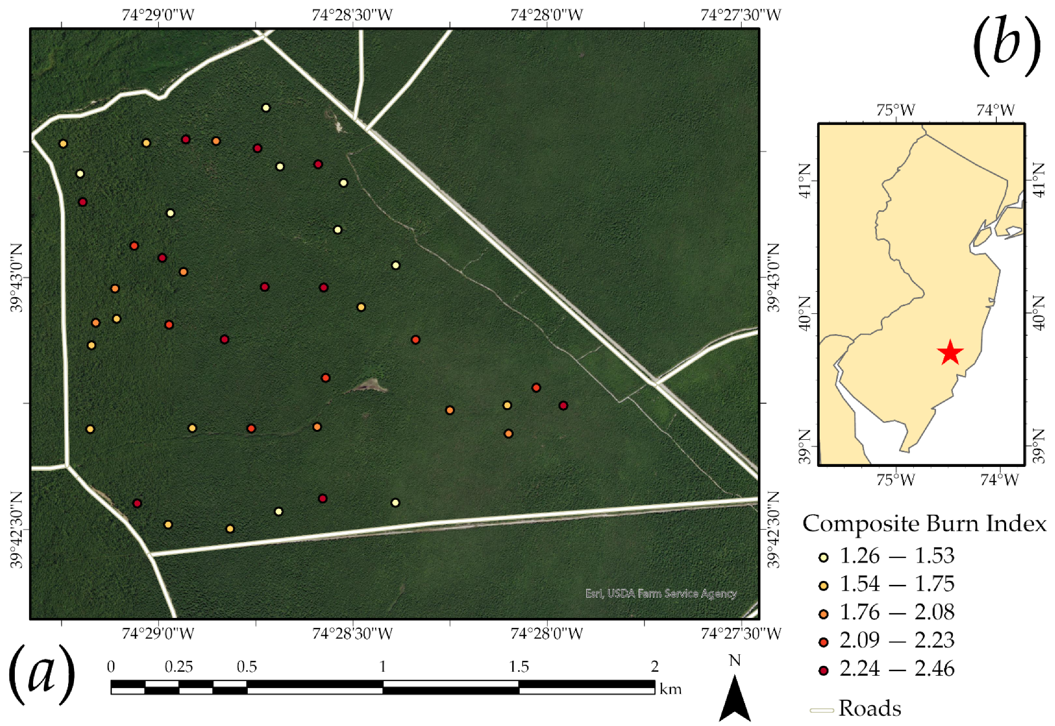
2.1. Study Area

The New Jersey Pinelands National Reserve (PNR) is a pyrogenic landscape that has a long history of landscape-scale prescribed burning as a wildfire management strategy. Upland and lowland forests dominated by pitch pine (Pinus rigida Mill.) characterize this 440,000-ha landscape and represent the greatest fuel hazard for wildfire management. Annually, approximately 10,000 ha are treated with prescribed fire in a mix of units that have been burned frequently and some that have been fire excluded for decades, while approximately 5000 ha also burn in wildfires [33]. Impacted forests rapidly regenerate via prolific dormant buds that are protected by bark or soil; however, the removal of biomass and sprouting regeneration can profoundly and durably create distinctive patterns in the three-dimensional structure of forest vegetation [18,34].
This study focused on a burn unit located in Wharton State Forest in southeastern Burlington County, New Jersey within the PNR. Overstory vegetation was dominated by pitch pine (Pinus rigida Mill.) and included infrequent subdominant post oaks (Quercus stellate Wangenh.), while blackjack oak (Quercus marilandica Muenchh.), suppressed or immature pitch pine, and immature post oak occupied the midstory. A mix of ericaceous shrubs (Vaccinium, Gaylussacia species primarily), laurels (Kalmia latifolia L. and angustifolia Kalm.), and shrub form oaks (Q. marilandica Muenchh. and ilicifolia Wangenh.) comprised the understory. Canopy height varied significantly across the unit between areas of a unique genetic provenance of pitch pine that exhibits short stature and exceptionally poor form [35,36,37]. The area was treated with mixed intensity prescribed fire in February 2021 but had not burned since June of 1939 or earlier.

2.2. Field Data Collection

Forty-three plots were randomly selected with the criteria that plots be at least 400 m apart from each other and 100 m from roads to facilitate separation of plots and prevent potential edge effects (Figure 1). Plots were marked in the field prior to burning, at which time pre-burn scans were collected with a BLK360 TLS (Leica Geosystems, Heerbrugg, Switzerland) following [19] as single return, single scans. GPS points at plot center with >2 m accuracy were collected at each plot using a Trimble GeoExplorer 6000 paired to a Tornado receiver (Trimble Inc., Sunnyvale, CA, USA). These data were collected during the dormant season in this region when foliage of deciduous shrubs was senescenced, between 25 February and 3 March 2021, or 3–9 days prior to burning.
The unit was then burned by the New Jersey Forest Fire Service on 6 March 2021. Post-burn scans were also collected as single return scans, between 15 and 22 March 2021, or 9–16 days after burning and still within the dormant season. Post-burn composite burn index (CBI) data were collected at plots within a 10 m radius shortly thereafter between 22 and 26 March 2021 (16–20 days post-burn) using the CBI field sheet provided in [11]. As per [11] this effort to collect CBI data reflects the objective of conducting an ‘initial assessment’ to identify first-order fire effects (i.e., chemical or physical changes relating to combustion processes) immediately following fire, in contrast to an ‘extended assessment’ that would be designed to observe first- and second-order fire effects (i.e., those that may occur later such as compositional change). In our assessment, half of the metrics pertaining to understory vegetation characteristics (i.e., foliage) were unavailable for observation during the dormant season for deciduous species present in plots and were thus omitted from observation in all plots. Basic tree data including species, height, and diameter were collected between 14 April and 5 August 2021. Tallied field data for each plot were then summarized to strata level ‘burn index’ results and then combined via averaging to develop plot-level CBI results as per the CBI method [11].

2.3. TLS Processing and Metric Generation

For each plot, both the pre- and post-fire single return, single-scan TLS datasets in e57 format were separately processed to derive summary metrics using the R [38] open-source data science environment and language and the lidR package [39]. First, points occurring within 10 m of the laser scanner were extracted to approximate the area in which CBI data were collected. Next, segmentation algorithms were used to remove trees from the point cloud and create two separate datasets, all returns and all non-tree returns, using the methods described by de Conto et al. [40]. The goal was to summarize the point cloud with and without trees present. Next, ground classification was applied to differentiate ground returns from all other returns using the cloth simulation function (CSF) as implemented in the lidR and the RCSF [41] packages. CSF classifies ground returns by modeling a rigid cloth surface defined by interconnected nodes within an inverted three-dimensional space (i.e., the point cloud is inverted, and the cloth surface is modeled above the points). This surface and its associated nodes are used to extract ground return points such that the cloth surface meets defined constraints of rigidness [42]. In this study, specifically, our process involved smoothing the surface to account for steep slopes with a threshold of 0.5 to specify the maximum distance from a cloth to potential ground returns and a distance of 0.5 between nodes in the cloth. Rigidness was maintained at the default value of 1 to allow for the modeling of rugged terrain and the time step was set to 0.65, which relates to how gravity is simulated in the model.
Once the ground classification was performed, lidR was used to normalize the point cloud to convert the elevation measurements to height above ground. This first required a triangulated irregular network (TIN) to be created from the classified ground returns followed by a rasterization of this surface to create a digital terrain model (DTM) of bare earth surface elevations. The ground elevation measurements from the DTM surface were then subtracted from the returns occurring above them.
All metrics were calculated from the classified and normalized point clouds. In order to calculate metrics that more closely aligned with the subcomponent forest strata of the CBI the point cloud was stratified as defined in Table 1. Similar to [20], we stratified point cloud data into 4 bins representative of forest subcomponent strata (i.e., substrate (L1), herbs and low shrubs (L2), tall shrubs (L3), and pole-size to tall trees (L4)); however, our bin definitions differed marginally from [20] to match those of CBI ([11]; Table 1). Next, summary statistics were calculated for all returns, ground returns, and not ground returns separated into the four height strata. The original CBI intermediate and tall tree categories were combined to a single tree group (L4).
Table 2 summarizes the features calculated. For ground-classified points, we simply calculated the number of ground returns and the percentage of all returns that were classified as ground. For all returns classified as not ground, we calculated total number, percent of total returns, and a variety of summary statistics for the height, or z, data including mean, median, standard deviation, entropy, vertical complexity index (VCI), skewness, kurtosis, percent of returns above the mean height, percent of returns occurring 2 m or higher above the ground, percentiles of z, and cumulative percent of returns above specified heights. Entropy is a measure of height diversity and was calculated using height bins of 0.25 m after Shannon [43]. VCI is a normalization of entropy and was calculated after [44]. In order to summarize the three-channel, visible camera (RGB) data, which were collected with the integrated camera and subsequently associated with each point return in the resulting point cloud in the original output files, we calculated the triangular greenness index (TGI [45]; see Equation (1)) and the visible atmospherically resistant index (VARI [46]; see Equation (2)), which are both vegetation indices that rely only on the visible spectral bands. We only used the RGB values associated with the point returns and did not make use of raster-based representations of the data. Although the camera data were not calibrated and the digital number values could not be converted to an estimate of spectral reflectance, we still included these metrics as a means to include spectral information in the regression models to complement point cloud-derived structural information. For each height bin, L1 through L4, we calculated the total number of returns; percent of not ground returns; mean, median, standard deviation, entropy, and the VCI from the z data; and TGI and VARI from the RGB data.
T G I = ( G r e e n 0.39 ) × ( R e d 0.61 ) × B l u e
V A R I = ( G r e e n R e d ) ( G r e e n + R e d B l u e )
A total of 80 metrics were calculated for each plot from the pre- and post-burn data separately. We then differenced each variable by subtracting the post-burn metrics from the pre-burn metrics to obtain differences.

2.4. Predictive Modeling and Assessment

Once the metric sets were generated and pre- and post-burn differences were calculated, multiple linear regression and machine learning were implemented to make predictions of CBI. All metrics were used to predict total CBI, as calculated from the entire point cloud without the trees removed. For the four components of CBI, only variables calculated from the associated strata, L1 through L4, were used. For predicting substrate (L1), herbaceous and small shrubs (L2), and tall shrubs (L3) CBI, metrics obtained from the point cloud with trees removed were used. For intermediate to large trees (L4) metrics were calculated with the trees included.
Due to the large number of predictor variables in comparison to the number of plots for predicting total CBI, we implemented a variable reduction method to select important variables. Specifically, we used the Boruta method as implemented by the Boruta package in R [47]. The Boruta method attempts to determine what features are relevant to the predictive task, as opposed to selecting a minimal optimal set of variables, as is common in other RF-based recursive feature elimination methods. It is a wrapper method that uses variable importance, as calculated by the RF algorithm, to assess the relevance of features relative to randomly generated “shadow variables”. The result is a distribution of Z-scores for each variable and a categorization of features as “important”, “unimportant”, or “tentatively important” [47,48]. In this study, we maintained all variables that were identified as “important”.
Three separate regression techniques were applied: multiple linear regression, random forest (RF) regression, and support vector machine (SVM) regression. Many methods are available to make predictions of continuous measures. We included multiple linear regression since this is a traditional, standard, and interpretable method that is often used as a benchmark for comparing or assessing other algorithms [49]. RF and SVM were explored since they are well established and operationalized and have been shown to generally provide strong performance for a wide variety of predictive modeling tasks. These methods have been widely adopted in the field of remote sensing and have even been integrated into commercial software packages, such as ArcGIS Pro [50,51,52,53]. Linear regression predicts the dependent variable, CBI in this case, using all independent variables and an ordinary least square fitting method. This results in the prediction of a y-intercept and coefficient for each predictor variable. Multiple linear regression assumes linear relationships between the dependent variable and all predictor variables, normal distribution of the dependent variable and model residuals, no or little multicollinearity between predictor variables, no spatial autocorrelation, and homoscedasticity (i.e., no changes in the variability in the model residuals with changes in the dependent variable) [49].
The RF algorithm is based on decision trees. Decision trees use binary partitioning of the input data to create more homogenous subsets. Recursive binary partitioning results in a series of decision rules, which can be used to make predictions of categorical or continuous variables. RF expands upon single decision trees by (1) incorporating many decision trees as an ensemble, (2) allowing only a subset of predictor variables to be available for determining a splitting rule at each node, and (3) using only a subset of the available training samples to produce each tree in the ensemble. The subset of training samples used in each tree is selected using bootstrapping, or random sampling with replacement. The goal is to generate a set of weak classifiers that are collectively strong due to reductions in correlation between the trees. RF has been shown to be robust to complex, noisy data and a large feature space [51,52,54].
SVM is a kernel-based method that attempts to determine the optimal hyperplane in a multidimensional feature space. This optimal boundary is defined based on the best or maximum separation or margin. Training samples nearest to the margins are used to define the hyperplane, as opposed to all examples, and these samples are termed support vectors. Since linear relationships may not exist in the original feature space, the problem can be projected to a higher-dimensional space using a kernel function where patterns may be more linear. This is known as the kernel trick [49,55,56,57]. In this study, we used the radial basis function (RBF) kernel.
All three regression methods were implemented using the caret [58] package in R. Model hyperparameters were optimized using a grid search and five-fold cross validation where the data are randomly split into five folds. Since only 43 plots were available, we used five folds as opposed to the more traditional ten folds to increase the number of samples assigned to each fold. Models are then generated using four folds, while the remaining fold is withheld for assessment. This process is repeated until each of the five folds have been withheld for assessment. For RF, the number of variables available for splitting at each node, or mtry, parameter was optimized. For SVM, the cost parameter (C) was optimized. The caret package acts as a wrapper for executing learning methods from other packages. Multiple linear regression uses the stats package [38], RF uses the randomForest package [59], and SVM uses the kernlab package [60].
Due to the limited number of plots, we did not withhold a dataset to validate the models. Instead, we used the results from the five-fold cross validation. Since the assessment is based only on the withheld data in each fold, this yields an assessment that is not impacted by overfitting [49]. Here, we report the highest average RMSE (Equation (3)) and R-squared (Equation (4)) calculated from the withheld folds during the hyperparameter optimization.
R M S E = ( y y ^ ) 2
R 2 = ( 1 R e s i d u a l   S u m   o f   S q u a r e s ) / ( T o t a l   S u m   o f   S q u a r e s )

3. Results

3.1. Field Data

Basal area of plots ranged from 9 to 25 m2/ha with stems per ha ranging from 541 to 3280, encompassing the ranges observed in other studies on this landscape [61,62,63,64]. Average diameter at breast height (DBH) in plots ranged from 8.1 to 19.1 cm and average stem height ranged from 4.5 m (e.g., areas dominated by dwarf pitch pine) to 11.2 m (see Appendix A for plot-level biometric summaries). Over 99% of trees were living prior to the burn.

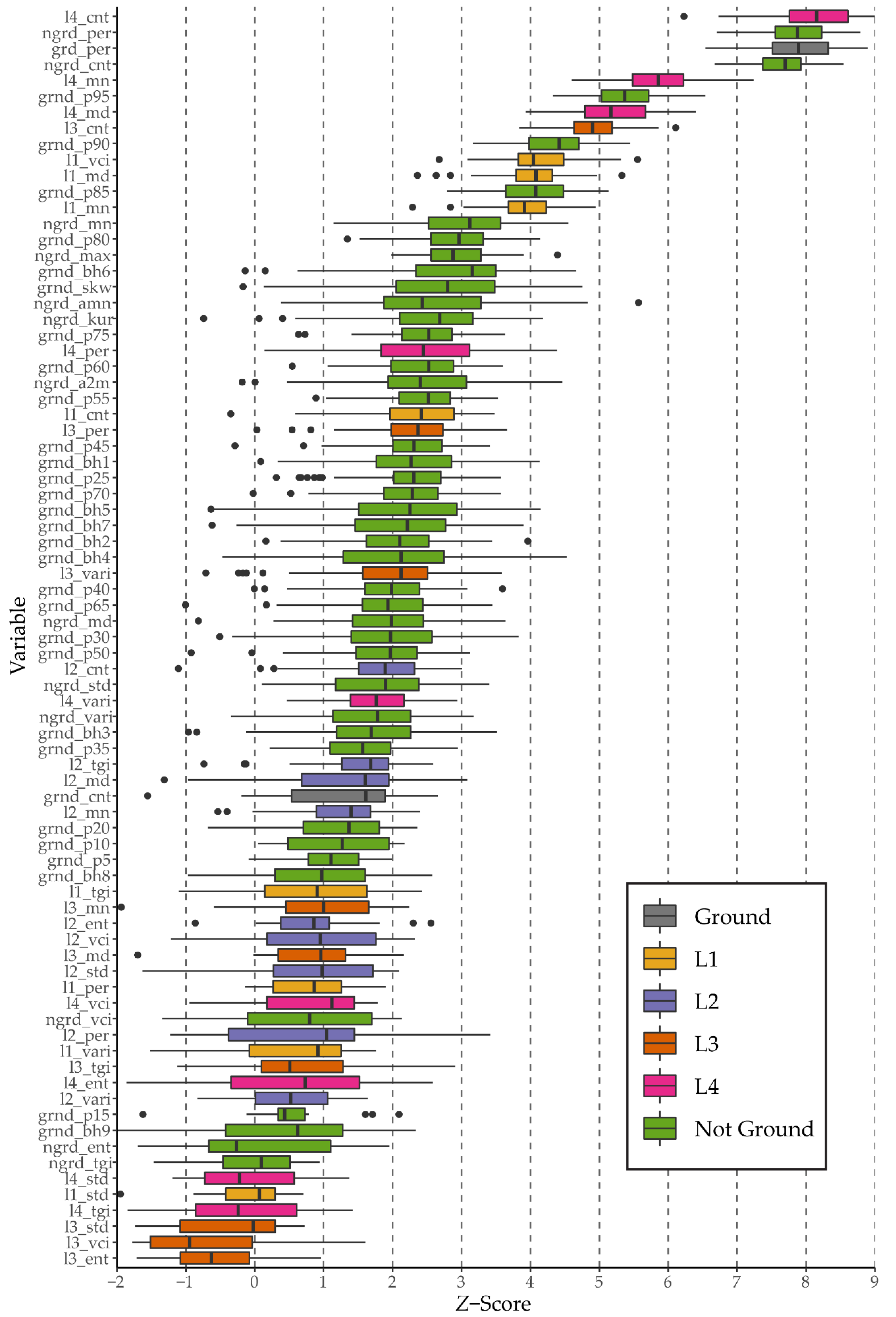
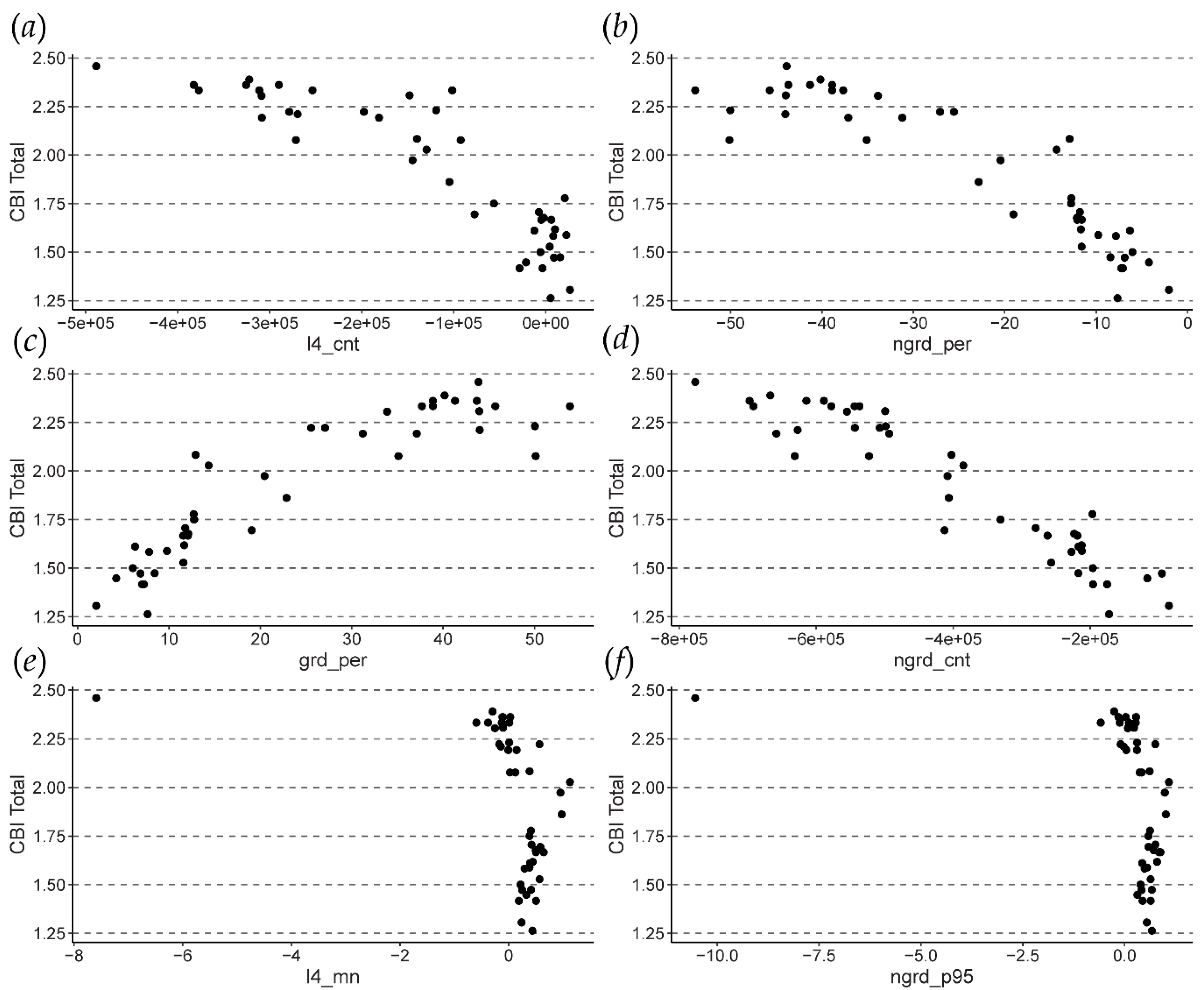
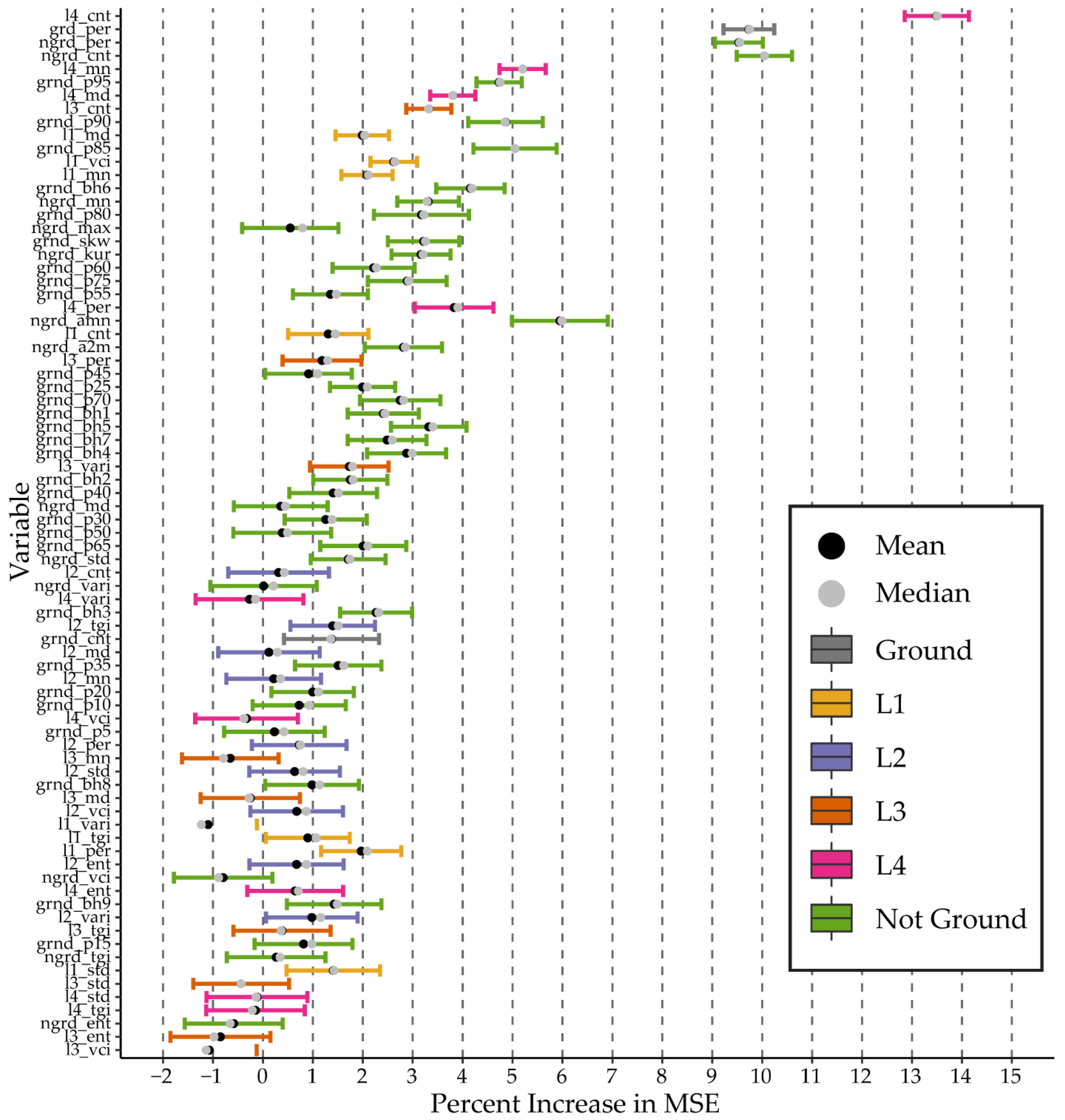
3.2. Variable Importance

Figure 2 shows the distribution of Z-scores, which provide an estimate of variable importance, generated using the Boruta method [10] for estimating total CBI. Given the small number of training samples and due to the stochastic nature of RF, variability in importance estimates is expected [65,66,67,68]. For comparison, Figure 3 shows variable importance estimated using the default RF importance estimation method, which is based on the mean increase in mean square error (MSE) when the predictor variable of interest is randomly permutated while all other variables are maintained [54]. In order to assess variability in the importance estimates, 500 separate RF models were generated to obtain mean and median measures for each variable along with standard deviations, shown in the figure using error bars. The variable order in Figure 3 is the same as in Figure 2 for comparison. Although the order of importance is not the same between the Boruta and standard RF importance estimation methods, similar patterns are observed, and several variables are highlighted as consistently important. It should be noted that traditional RF-based variable importance estimates are generally interpreted as marginal importance, or an assessment of variable importance not impacted by other variables in the feature space [54,65,66,67,68].
Using the Boruta method, several variables were noted to be of importance. The top six ranked variables were as follows (ρ = Spearman’s rho): l4_cnt (ρ = −0.87), ngrd_per (ρ = −0.91), grd_per (ρ = 0.91), ngrd_cnt (ρ = −0.92), l4_mn (ρ = −0.64), and grnd_p95 (ρ = −0.64). Spearman’s rho, which is based on ranks, was provided as a metric of correlation between total CBI and these specific predictor variables since we were interested in correlation in general as opposed to linear correlation. The relationships between total CBI and each of these variables are shown in Figure 4, which generally suggest strong correlations with total CBI. For predicting total CBI specifically, variables calculated using the entire set of not ground returns and those calculated using just not ground returns in L4 tended to show higher importance in the model than variables calculated using not ground returns in the other three strata. This suggests that CBI for trees has a larger impact or contribution on overall CBI than the substrate, herbaceous and small shrubs, and large shrubs strata.

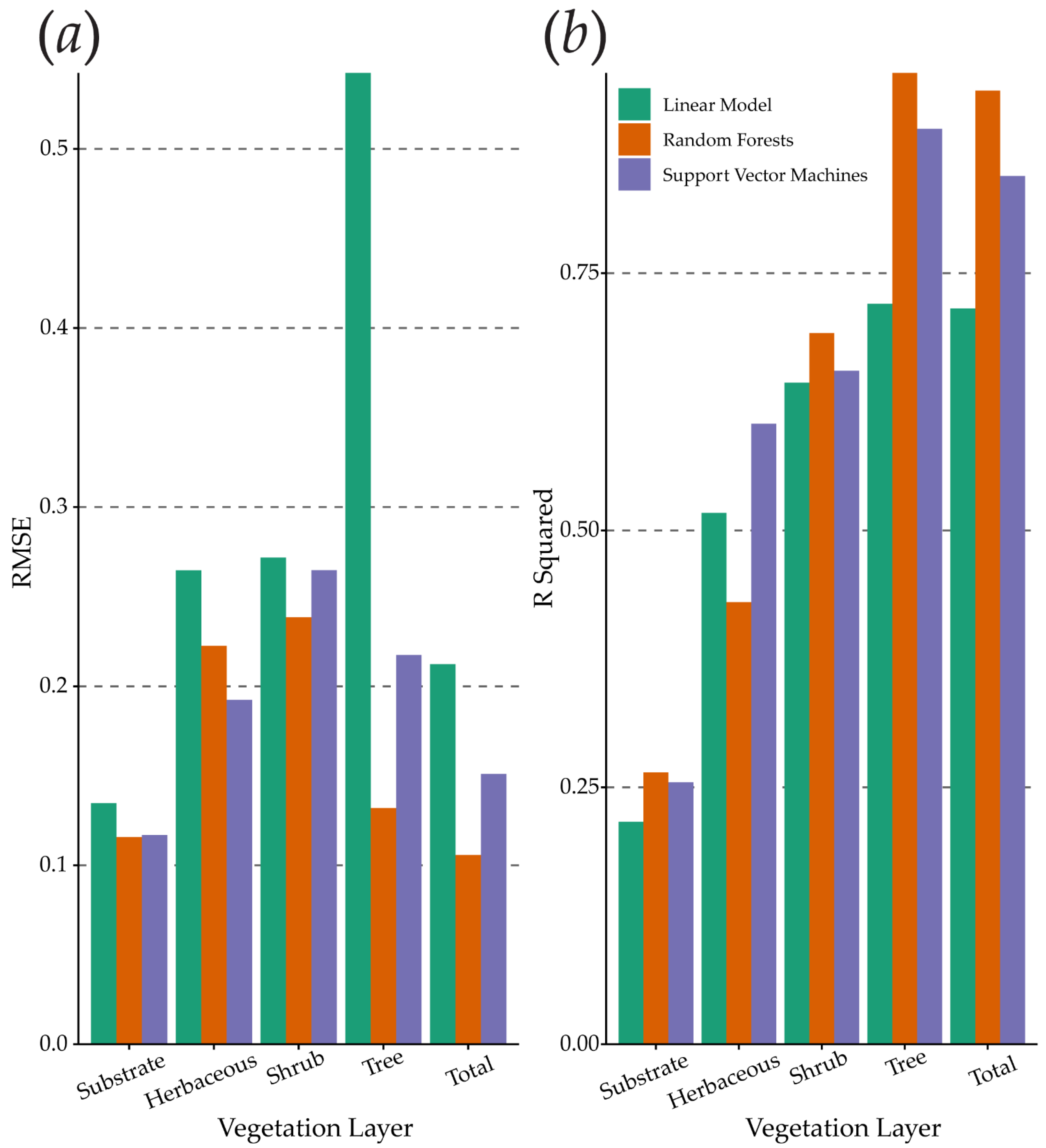
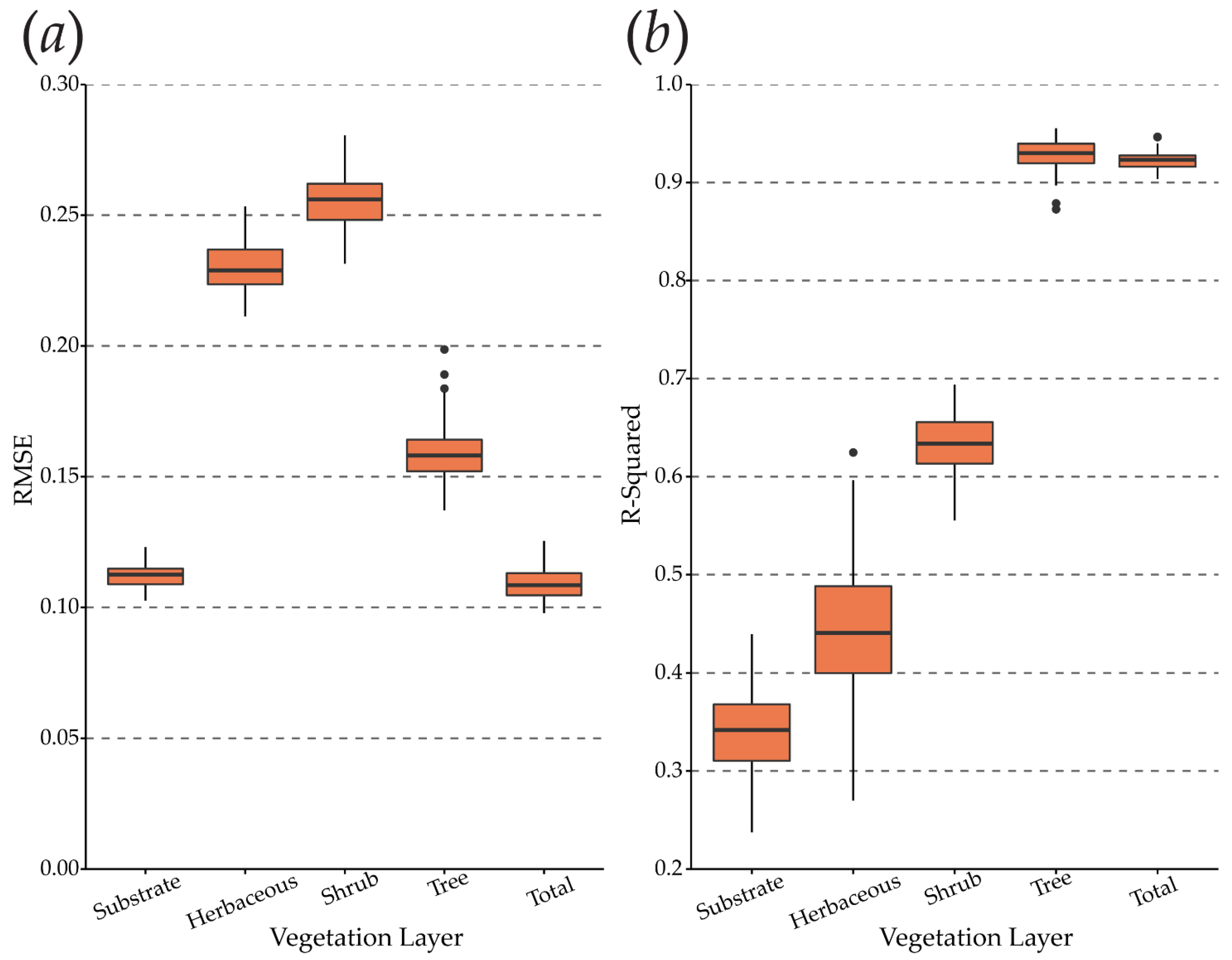
3.3. Model Performance

Figure 5 shows the RMSE and R-squared metrics estimated from the withheld folds for each prediction by strata for each algorithm. Generally, the machine learning methods outperformed multiple linear regression based on both metrics. Or, RMSE tended to be lower and R-squared higher for the SVM and RF models. We attribute this to the ability of these algorithms to model more complex, non-linear patterns and relationships within the feature space. Generally, RF outperformed SVM in the calculations.
Generally, total plot CBI and CBI for trees was predicted more accurately than CBI for the other strata. This makes sense for the substrate and herbaceous layers since the majority of the provided variables relate to distribution of the z measurements, which is less meaningful for these strata. The lower predictive performance for shrubs was more surprising. This could be related to occlusion of shrub features by tree trunks or due to the characteristics of the fire.
It should be noted that due to the stochastic nature of the RF algorithm, results and predictive performance may vary between model runs. This can be especially true when using a small training set [49,54]. In order to assess the consistency of the RF predictions, we trained 50 separate models for each vegetation layer or CBI strata. The results of this experiment are shown in Figure 6. Generally, model performance was consistent, especially for strata that were predicted with higher accuracies (i.e., trees and total CBI). However, due to this variability, the relative performance between RF and SVM may vary.
Other than overall accuracy and predictive performance, it is also important to consider the suitability of modeling techniques for specific tasks. In this study in particular, it was important to assess assumptions of multiple linear regression. We made use of diagnostic tests and visualizations made available by the car package in R [69] and specifically investigated the total CBI prediction using the variable subset suggested by Boruta. Visual assessment with a Q-Q plot suggested normality of model residuals and minimal issues of skewness or kurtosis while the Score Test for Non-Constant Error Variance suggested no issues associated with homogeneity of variance (p-value = 0.289). Partial residual plots showed some non-linear relationships between total CBI and specific variables. The largest issue is related to multicollinearity between many of the predictor variables. In summary, given the complexity of the feature space, nonlinear relationships, and multicollinearity between predictor variables, we argue that multiple linear regression is not an optimal method for this task. So, other than just consistently lower predictive performance in comparison to RF and SVM, violation of model assumption further supports the use of nonparametric machine learning for this task. If multiple linear regression is desired, perhaps to obtain more interpretable results, some preprocessing would be required.
It should also be noted that machine learning methods do require some specific considerations. For example, a large number of predictor variables and a small number of training samples can result in overfitting in some cases. Additionally, imbalanced training data for classification problems can result in poor predictive performance for the rarer classes while training samples that do not capture the full variability or range of a continuous dependent variable may result in poorer predictions due to extrapolation errors. For RF specifically, it has been shown that measures of importance can be misleading when predictor variables are highly correlated or variables are measured on different scales or have a different number of levels, in the case of categorical variables. Although model predictive performance may not be greatly impacted by collinearity, such issues can complicate variable importance assessment and make model interpretation more difficult [49,51,53,54,65,66,67,68,70,71].
Figure 7 compares different subsets of features for predicting each strata and total plot CBI. Generally, the best performance was obtained using all predictor variables or just those derived from the TLS data. Using just the camera-derived variables of TGI and VARI generally yielded poor results. Using just the metrics from the post-burn data, as opposed to the difference, yielded slightly reduced performance, but also outperformed the camera-only models.

4. Discussion

Our study provides a replicable workflow and numerous variables relating to forest structure and true color RGB values that can be used as alternative criteria for refencing burn severity (e.g., dNBR or other indices) consistently in any landscape for both prescribed fire and wildfire. The TLS approach presented is beneficial in that it is fast (~4 min to scan), consistent, repeatable, provides a far more detailed depiction of forest conditions than CBI, is relatively inexpensive with regard to the cost of current forest monitoring programs, and data can also be used to inventory fuels with greater richness and speed than traditional inventorying methods [19]. In contrast to the typical 23 indirectly observed variables that are integrated into CBI calculations, the 70 TLS-based variables and 10 RGB-based variables presented in this study demonstrate how our approach can be used to characterize forest structure and spectral conditions. Further, we demonstrate how machine learning can greatly improve predictions that integrate many predictor variables, compared to the more traditional multiple linear regression. These methods were able to model more complex relationships and patterns in the data in comparison to linear regression. Overall, including all available predictor variables did not improve the prediction of total plot CBI in comparison to just using the TLS-derived measures when using the RF algorithm (Figure 4); however, at the strata level, fit was best when predictions were made with the SVM algorithm. The RGB data improved predictions in some but not all cases (Figure 7), but alone poorly predicted total plot CBI. Compared to previous studies that have attempted to predict plot-level or strata-specific burn severity from TLS data with poor to moderate results (R2 = 0.05–0.75 [20,21]), our approach produced substantially stronger results (R2 = 0.70–0.94, Figure 7). Our study differed in that it leveraged the richness of TLS datasets by generating far more variables related to vegetation structure heterogeneity and then utilized machine learning to generate predictions. The predictions generated in this study also differed in their incorporation of RGB variables which are linked to non-structural vegetation effects (i.e., charring, necrosis of vegetation).
Our results highlight important challenges of observing burn severity linked to plant phenology that have yet to be reconciled in existing methods or the method we have tested. CBI field observations are heavily reliant on color proportions in the burned environment (e.g., green foliage, yellow/brown foliage, and char) to infer vegetation damage or mortality; however, these observations can be challenging to infer during leaf-off conditions immediately after fires in the dormant season. In our study area, the understory and mid-story compositions were primarily deciduous and were dormant during our study and corresponded with poor strata-specific predictions of CBI; however, the overstory was evergreen and in that strata predictions from RGB were substantially better (Figure 6). RGB data may be more useful for initial burn severity assessments following growing season fires or for extended assessments of dormant season burn severity during the growing season (i.e., after vegetation has seeded or resprouted). Similarly, CBI may also be a more useful for extended assessments when fire effects of dormant season burns are difficult to assess until vegetation has leafed out in the spring, although managers may not always have the flexibility to wait many months before assessing the impacts of their burns. These phenological considerations are particularly important for managers and researchers in regions such as the eastern US where the majority of prescribed burning occurs in the dormant season, or when comparing severity of fires that occurred across both leaf-on and leaf-off conditions.
Other studies have shown that ALS can identify important structural variation in fire effects from both prescribed fires and wildfires and that dNBR is highly correlated with structural change in the forest [8,18]. However, this study and previous works highlight that despite correlations between total plot CBI and dNBR, total plot CBI is a poor reference for understory fire effects because of its bias towards the canopy and focus on observation variables that poorly reflect physical change in the understory. We also highlight that CBI is performed after the fire, where the observer makes assumptions about the pre-fire vegetation conditions. As such, CBI only considers the post-fire state and as such, is not a true change detection method. This has limited capacity to rigorously infer physical change on vegetation from fire. Development of a TLS-based field approach could replace the CBI method for validation of dNBR mapping products and provide a more robust reference of fire effects in the forest, especially during low-to-moderate severity fires where fire effects are focused on the understory.
Our study had shortcomings that can be considered in the planning of future studies to maximize the usefulness of data and reduce confounding factors. First, we point out that we exported our TLS data in e57 format and then converted that data to laz format on the basis that it required less storage space than other formats and aligned with our existing workflows. However, since conducting this study, it has been learned that e57 format permanently truncates important non-return data collected by the BLK360, reducing the richness of the data and weakening the user’s ability to interpret potential relationships with field observations of vegetation [32]. Alternatively, we suggest future users consider following Stovall and Atkins’ recommendation of exporting data in ptx format, which preserves the complete dataset of both return and non-return information [32]. There are also additional inherent challenges associated with using RGB data that may have affected our results and should be considered in future studies. Inconsistencies in lighting across plots during the 360-degree data collection are impossible to avoid and thus variable shading may be a confounding factor that reduces predictive power of these variables. As previously stated, the RGB data in our study were uncalibrated; however, digital image calibration processes using color calibration panels or discs has improved interpretation or characterization of vegetation for other purposes (e.g., fine-scale analyses of agricultural field crop foliar conditions) and may be useful for improving burn severity prediction with 360-degree RGB imagery in the future [72,73]. It should be noted that these approaches require calibration panels or discs to be placed in the scene during image capture, which we did not do, and thus post hoc calibration of RGB data in this study was not possible.
Monitoring of prescribed fire and wildfire effects is a critical component of determining management needs and evaluating the ecological and fuel effects of management treatments and responses. Forest resource managers typically use remotely sensed data and indices of burn severity as an alternative to directly observing fire effects. Wall-to-wall remote sensing of burn severity typically provides two-dimensional maps that can indirectly measure loss of organic matter from fire when calibrated with field data, but alone are of insufficient resolution to predict change throughout the canopy profile [8]. However, the primary method for observing burn severity in the field (i.e., CBI) has multiple documented weaknesses that have yet to be improved upon, especially for below canopy biomass. These weaknesses are rooted in the indirect nature of observations of forest biomass change.
TLS and associated RGB data can be very useful for quantifying forest structure and its change, but also can be challenging to use. There is complexity in merging multiple- TLS and RGB scan collections due to different sensor positions, identification of similar features in complex vegetation, issues of occlusion when only single-return data are used. We avoided these issues by collecting single scans at each plot before and after burning, and by utilizing point cloud summary information rather than differencing point clouds themselves. Despite the occlusion issues that can arise from using single return TLS units, multiple return TLS data can also present challenges to the user if outputs do not differentiate first returns from other returns because assessing the probability of returns encountering vegetation becomes intractable. Similarly, the spherical probability pattern of TLS pulses encountering vegetation is a challenging factor of 360-degree data acquisitions that can complicate interpretation analyses that are dependent on the density of soft features (e.g., foliage) rather than the presence or absence of hard features (e.g., the walls of buildings), yet have remained largely overlooked. This challenge contrasts with the use of ALS data or more simplistic upward facing TLS units where data where the directionality of data sampling is uniform and thus the probability of laser pulses encountering vegetation is easier to interpret. Referencing the RGB data to the point measurements, errors in tree removal necessary for objectively analyzing understory and midstory vegetation, ground classification and normalization methods, and lack of metadata for some cheaper sensors are additional challenges that need to be considered when using our approach to estimate burn severity.
This study demonstrated how TLS and RGB data can be used to quantify burn severity following a dormant season fire in a pitch-pine dominated forest; however, future research that builds on this by conducting similar studies in forests of other species compositions and during growing season (e.g., leaf-on) conditions will be extremely informative for expanding the use of this approach among managers and researchers. Similarly, research that explores the spherical influence of scan patterns on TLS data probability distributions would improve the validation and interpretation of TLS-based results, whether for burn severity estimation or other purposes (e.g., vegetation structure monitoring). Additionally, future research can utilize the structural and reflectance variables presented in the manuscript to predict dNBR and investigate the potential for TLS and RGB-based burn severity data to replace CBI. This would be extremely beneficial in enhancing manager capacity to monitor fire treatment and utilize monitoring data to inform management and can be incorporated with TLS-based fuels monitoring strategies [19,29].

5. Conclusions

Our study demonstrated the use of terrestrial laser scanner data in the New Jersey PNR to characterize the forest structure before and after burns to create metrics of change based on loss of organic matter to estimate burn severity. The results of this work indicate that this approach is fast, consistent, and repeatable. In addition, it requires little field expertise or training, and data can also be used to inventory fuels with additional calibration in ways that meet the requirements of new physics-based fire behavior simulators.
Comparison of data analysis algorithms showed that the random forests machine learning algorithm provided substantially better results than a multiple linear regression approach, but also highlighted inconsistencies in the correlation between CBI data and loss of organic matter between forest strata. Canopy CBI and TLS burn severity had the highest correlation, while tall shrubs had the weakest despite being closest to the scanner and therefore less occluded than other layers. This result suggests future research should investigate replacing or modifying CBI with a TLS approach that is demonstrably more consistent and tractable.
These results have important implications for forest resource managers. The opportunity to increase the quality and pace of burn severity observations and integrate with inventorying and modeling needs documented here could contribute to the updating of field-based fuels and fire effects monitoring to better meet current needs of forest resource managers. Similarly, these results demonstrate the potential for this approach to define burn severity at prescribed burns in terms of metrics based on loss in organic matter in specific strata, which are more informative than strata-specific CBI metrics. These results also highlight the advantage of incorporating computational skills like machine learning into wildland fire management, particularly in low to moderate severity fires or frequently burned systems where fire effects are generally found beneath the canopy.

Author Contributions

Conceptualization, M.R.G., A.E.M., N.S.S. and E.L.L.; methodology, A.E., M.R.G., L.A.G. and A.E.M.; formal analysis, A.E.M. and L.A.G.; investigation, M.R.G., A.E.M., A.E., E.L.L. and L.A.G.; resources, A.E.M., N.S.S. and E.L.L.; data curation, A.E. and L.A.G.; writing—original draft preparation, M.R.G., A.E., N.S.S. and E.L.L.; writing—review and editing, N.S.S. and E.L.L.; visualization, M.R.G. and A.E.M.; supervision, M.R.G.; project administration, N.S.S.; funding acquisition N.S.S., A.E.M., and M.R.G. All authors have read and agreed to the published version of the manuscript.

Funding

This project was funded by the USDA Forest Service Northern Research Station through joint venture agreement 20-JV-11242306-069.

Informed Consent Statement

Not applicable.

Data Availability Statement

The data presented in this study are available on request from the corresponding author.

Acknowledgments

We thank New Jersey Forest Fire Service, especially Trevor Raynor and John Earlin for their field expertise and for providing the opportunity to conduct this study. We thank the New Jersey Division of Parks and Forestry and the or access to portions of the burn unit on Wharton State Forest. We thank Julia Defeo, Richard Strittmatter, and Matthew Patterson for their help in the field. The use of trade, firm, or corporation names in this article is for the information and convenience of the reader. Such use does not constitute an official endorsement or approval by the U.S. Department of Agriculture or the Forest Service of any product or service to the exclusion of others that may be suitable.

Conflicts of Interest

The authors declare no conflict of interest.

Appendix A

Table A1. Summary of Biometric Data for Field Plots.
Basal Area (m2/ha)Stems/ha (n)DBH (cm; Mean ± 1SD)Height (m; Mean ± 1SD)
9.78289.4 ± 8.34.6 ± 2.9
15.124528.2 ± 3.44.5 ± 1.6
17.028348.1 ± 3.54.5 ± 1.6
17.624208.8 ± 3.84.8 ± 2.0
18.325808.7 ± 3.94.6 ± 2.0
19.425489.2 ± 3.54.9 ± 1.8
19.554119.1 ± 10.011.2 ± 4.6
20.898714.7 ± 7.57.5 ± 4.2
22.2127412.7 ± 7.97.7 ± 4.1
22.6108313.6 ± 9.18.7 ± 4.9
22.8219710.4 ± 5.06.5 ± 3.1
23.7235710.5 ± 4.26.4 ± 2.3
23.9121013.5 ± 8.37.6 ± 4.4
23.932808.8 ± 3.95.2 ± 2.1
24.7159212.1 ± 7.28.2 ± 4.5
24.9114613.4 ± 10.08.7 ± 5.5
25.098715.1 ± 9.98.1 ± 5.1
26.3114614.1 ± 9.98.7 ± 6.2
26.7197511.7 ± 6.07.4 ± 3.5
26.7105114.6 ± 10.69.2 ± 6.1
26.8149713.8 ± 6.38.4 ± 3.6
26.9245210.3 ± 5.96.9 ± 3.3
27.0194312.1 ± 5.67.2 ± 3.1
27.6117814.5 ± 9.59.2 ± 5.4
27.9187911.9 ± 6.98.1 ± 4.3
28.098716.9 ± 8.910.3 ± 4.5
28.1178312.6 ± 6.59.0 ± 4.7
28.7127414.6 ± 8.710.2 ± 4.9
29.6105117.0 ± 8.59.7 ± 4.5
30.2127413.9 ± 10.68.2 ± 4.9
30.3222911.7 ± 6.37.4 ± 3.7
30.3108314.8 ± 11.99.3 ± 6.5
30.4140113.7 ± 9.59.4 ± 5.4
30.9194312.8 ± 6.38.3 ± 3.3
31.6175213.1 ± 7.68.0 ± 4.3
32.0181513.2 ± 7.28.8 ± 4.2
32.0197512.2 ± 7.77.8 ± 4.4
32.2140115.1 ± 8.110.6 ± 4.2
32.3165614.1 ± 7.29.9 ± 4.0
32.6117817.5 ± 6.913.2 ± 4.2
33.6207012.7 ± 6.97.8 ± 4.1
33.8165614.4 ± 7.39.0 ± 4.1
35.1178314.0 ± 7.69.6 ± 4.7

References

  1. Kane, V.R.; Cansler, C.A.; Povak, N.A.; Kane, J.T.; McGaughey, R.J.; Lutz, J.A.; Churchill, D.J.; North, M.P. Mixed severity fire effects within the Rim fire: Relative importance of local climate, fire weather, topography, and forest structure. For. Ecol. Manag. 2015, 358, 62–79. [Google Scholar] [CrossRef] [Green Version]
  2. McLauchlan, K.K.; Higuera, P.E.; Miesel, J.; Rogers, B.M.; Schweitzer, J.; Shuman, J.K.; Tepley, A.J.; Varner, J.M.; Veblen, T.T.; Adalsteinsson, S.A. Fire as a fundamental ecological process: Research advances and frontiers. J. Ecol. 2020, 108, 2047–2069. [Google Scholar] [CrossRef]
  3. Simard, S. Fire severity, changing scales, and how things hang together. Int. J. Wildland Fire 1991, 1, 23–34. [Google Scholar] [CrossRef]
  4. Hardy, C.C. Wildland fire hazard and risk: Problems, definitions, and context. For. Ecol. Manag. 2005, 211, 73–82. [Google Scholar] [CrossRef]
  5. Keeley, J.E. Fire intensity, fire severity and burn severity: A brief review and suggested usage. Int. J. Wildland Fire 2009, 18, 116–126. [Google Scholar] [CrossRef]
  6. Bond, W.J.; Keeley, J.E. Fire as a global ‘herbivore’: The ecology and evolution of flammable ecosystems. Trends Ecol. Evol. 2005, 20, 387–394. [Google Scholar] [CrossRef] [PubMed]
  7. Hardy, C.C.; Schmidt, K.M.; Menakis, J.P.; Sampson, R.N. Spatial data for national fire planning and fuel management. Int. J. Wildland Fire 2001, 10, 353–372. [Google Scholar] [CrossRef]
  8. Skowronski, N.S.; Gallagher, M.R.; Warner, T.A. Decomposing the Interactions between Fire Severity and Canopy Fuel Structure Using Multi-Temporal, Active, and Passive Remote Sensing Approaches. Fire 2020, 3, 7. [Google Scholar] [CrossRef] [Green Version]
  9. Meyer, M.D.; Long, J.; Safford, H.; Sawyer, S.; North, M.; White, A. Chapter 1: Principles of postfire restoration in Meyer. In Postfire Restoration Framework for National Forests in California; Gen. Tech. Rep. PSW-GTR-270; Department of Agriculture, Forest Service, Pacific Southwest Research Station: Albany, CA, USA, 2021; pp. 1–30. [Google Scholar]
  10. Miller, J.D.; Yool, S.R. Mapping forest post-fire canopy consumption in several overstory types using multi-temporal Landsat TM and ETM data. Remote Sens. Environ. 2002, 82, 481–496. [Google Scholar] [CrossRef]
  11. Key, C.H.; Benson, N.C. Landscape assessment (LA). In FIREMON: Fire effects monitoring and inventory system; Gen. Tech. Rep. RMRS-GTR-164-CD; US Department of Agriculture, Forest Service, Rocky Mountain Research Station: Fort Collins, CO, USA, 2006; 164, p. LA-1-55. [Google Scholar]
  12. Garcia, M.J.L.; Caselles, V. Mapping burns and natural reforestation using Thematic Mapper data. Geocarto Int. 1991, 6, 31–37. [Google Scholar] [CrossRef]
  13. French, N.H.; Kasischke, E.S.; Hall, R.J.; Murphy, K.A.; Verbyla, D.L.; Hoy, E.E.; Allen, J.L. Using Landsat data to assess fire and burn severity in the North American boreal forest region: An overview and summary of results. Int. J. Wildland Fire 2008, 17, 443–462. [Google Scholar] [CrossRef]
  14. Gallagher, M.R.; Skowronski, N.S.; Lathrop, R.G.; McWilliams, T.; Green, E.J. An Improved Approach for Selecting and Validating Burn Severity Indices in Forested Landscapes. Can. J. Remote Sens. 2020, 46, 100–111. [Google Scholar] [CrossRef]
  15. Hiers, J.K.; O’Brien, J.J.; Varner, J.M.; Butler, B.W.; Dickinson, M.; Furman, J.; Gallagher, M.; Godwin, D.; Goodrick, S.L.; Hood, S.M. Prescribed fire science: The case for a refined research agenda. Fire Ecol. 2020, 16, 11. [Google Scholar] [CrossRef] [Green Version]
  16. Kolden, C.A.; Smith, A.M.S.; Abatzoglou, J.T. Limitations and utilisation of Monitoring Trends in Burn Severity products for assessing wildfire severity in the USA. Int. J. Wildland Fire 2015, 24, 1023–1028. [Google Scholar] [CrossRef]
  17. Picotte, J.J.; Bhattarai, K.; Howard, D.; Lecker, J.; Epting, J.; Quayle, B.; Benson, N.; Nelson, K. Changes to the Monitoring Trends in Burn Severity program mapping production procedures and data products. Fire Ecol. 2020, 16, 16. [Google Scholar] [CrossRef]
  18. Warner, T.A.; Skowronski, N.S.; La Puma, I. The influence of prescribed burning and wildfire on lidar-estimated forest structure of the New Jersey Pinelands National Reserve. Int. J. Wildland Fire 2020, 29, 1100–1108. [Google Scholar] [CrossRef]
  19. Pokswinski, S.; Gallagher, M.R.; Skowronski, N.S.; Loudermilk, E.L.; Hawley, C.; Wallace, D.; Everland, A.; Wallace, J.; Hiers, J.K. A simplified and affordable approach to forest monitoring using single terrestrial laser scans and transect sampling. MethodsX 2021, 8, 101484. [Google Scholar] [CrossRef] [PubMed]
  20. Kato, A.; Moskal, L.M.; Batchelor, J.L.; Thau, D.; Hudak, A.T. Relationships between Satellite-Based Spectral Burned Ratios and Terrestrial Laser Scanning. Forests 2019, 10, 444. [Google Scholar] [CrossRef] [Green Version]
  21. Philipp, M.B.; Levick, S.R. Exploring the potential of C-Band SAR in contributing to burn severity mapping in tropical savanna. Remote Sens. 2020, 12, 49. [Google Scholar] [CrossRef] [Green Version]
  22. Zhu, X.; Skidmore, A.K.; Wang, T.; Liu, J.; Darvishzadeh, R.; Shi, Y.; Premier, J.; Heurich, M. Improving leaf area index (LAI) estimation by correcting for clumping and woody effects using terrestrial laser scanning. Agric. For. Meteorol. 2018, 263, 276–286. [Google Scholar] [CrossRef]
  23. Calders, K.; Newnham, G.; Burt, A.; Murphy, S.; Raumonen, P.; Herold, M.; Culvenor, D.; Avitabile, V.; Disney, M.; Armston, J. Nondestructive estimates of above-ground biomass using terrestrial laser scanning. Methods Ecol. Evol. 2015, 6, 198–208. [Google Scholar] [CrossRef]
  24. Greaves, H.E.; Vierling, L.A.; Eitel, J.U.; Boelman, N.T.; Magney, T.S.; Prager, C.M.; Griffin, K.L. Estimating aboveground biomass and leaf area of low-stature Arctic shrubs with terrestrial LiDAR. Remote Sens. Environ. 2015, 164, 26–35. [Google Scholar] [CrossRef]
  25. Danson, F.M.; Hetherington, D.; Morsdorf, F.; Koetz, B.; Allgower, B. Forest canopy gap fraction from terrestrial laser scanning. IEEE Geosci. Remote Sens. Lett. 2007, 4, 157–160. [Google Scholar] [CrossRef] [Green Version]
  26. Li, Y.; Guo, Q.; Su, Y.; Tao, S.; Zhao, K.; Xu, G. Retrieving the gap fraction, element clumping index, and leaf area index of individual trees using single-scan data from a terrestrial laser scanner. ISPRS J. Photogramm. Remote Sens. 2017, 130, 308–316. [Google Scholar] [CrossRef]
  27. Disney, M.; Burt, A.; Wilkes, P.; Armston, J.; Duncanson, L. New 3D measurements of large redwood trees for biomass and structure. Sci. Rep. 2020, 10, 16721. [Google Scholar] [CrossRef] [PubMed]
  28. Ye, W.; Qian, C.; Tang, J.; Liu, H.; Fan, X.; Liang, X.; Zhang, H. Improved 3D stem mapping method and elliptic hypothesis-based DBH estimation from terrestrial laser scanning Data. Remote Sens. 2020, 12, 352. [Google Scholar] [CrossRef] [Green Version]
  29. Rowell, E.; Loudermilk, E.L.; Hawley, C.; Pokswinski, S.; Seielstad, C.; Queen, L.; O’brien, J.J.; Hudak, A.T.; Goodrick, S.; Hiers, J.K. Coupling terrestrial laser scanning with 3D fuel biomass sampling for advancing wildland fuels characterization. For. Ecol. Manag. 2020, 462, 117945. [Google Scholar] [CrossRef]
  30. Wilson, N.; Bradstock, R.; Bedward, M. Detecting the effects of logging and wildfire on forest fuel structure using terrestrial laser scanning (TLS). For. Ecol. Manag. 2021, 488, 119037. [Google Scholar] [CrossRef]
  31. Wilkes, P.; Lau, A.; Disney, M.; Calders, K.; Burt, A.; de Tanago, J.G.; Bartholomeus, H.; Brede, B.; Herold, M. Data acquisition considerations for terrestrial laser scanning of forest plots. Remote Sens. Environ. 2017, 196, 140–153. [Google Scholar] [CrossRef]
  32. Stovall, A.E.; Atkins, J.W. Assessing low-cost terrestrial laser scanners for deriving forest structure parameters. Preprints 2021. [Google Scholar] [CrossRef]
  33. Gallagher, M. Monitoring Fire Effects in the New Jersey Pine Barrens Using Burn Severity Indices; Dissertation; Rutgers, The State University of New Jersey: New Brunswick, NJ, USA, 2017. [Google Scholar]
  34. Skowronski, N.S.; Clark, K.L.; Duveneck, M.; Hom, J. Three-dimensional canopy fuel loading predicted using upward and downward sensing LiDAR systems. Remote Sens. Environ. 2011, 115, 703–714. [Google Scholar] [CrossRef]
  35. Lutz, H.J. Ecological Relations in the Pitch Pine Plains of Southern New Jersey; Yale University: New Haven, CT, USA, 1934. [Google Scholar]
  36. Givnish, T.J. Serotiny, geography, and fire in the Pine Barrens of New Jersey. Evolution 1981, 35, 101–123. [Google Scholar] [CrossRef] [Green Version]
  37. Ledig, F.T.; Hom, J.L.; Smouse, P.E. The evolution of the New Jersey pine plains. Am. J. Bot. 2013, 100, 778–791. [Google Scholar] [CrossRef]
  38. R Core Team. R: A Language and Environment for Statistical Computing; R Foundation for Statistical Computing: Vienna, Austria, 2020. [Google Scholar]
  39. Roussel, J.-R.; Auty, D.; Coops, N.C.; Tompalski, P.; Goodbody, T.R.; Meador, A.S.; Bourdon, J.-F.; de Boissieu, F.; Achim, A. lidR: An R package for analysis of Airborne Laser Scanning (ALS) data. Remote Sens. Environ. 2020, 251, 112061. [Google Scholar] [CrossRef]
  40. De Conto, T.; Olofsson, K.; Görgens, E.B.; Rodriguez, L.C.E.; Almeida, G. Performance of stem denoising and stem modelling algorithms on single tree point clouds from terrestrial laser scanning. Comput. Electron. Agric. 2017, 143, 165–176. [Google Scholar] [CrossRef]
  41. Roussel, J.; Qi, J. RCSF: Airborne LiDAR Filtering Method Based on Cloth Simulation. R Package Version 2018, 1, 1. [Google Scholar]
  42. Zhang, W.; Qi, J.; Wan, P.; Wang, H.; Xie, D.; Wang, X.; Yan, G. An easy-to-use airborne LiDAR data filtering method based on cloth simulation. Remote Sens. 2016, 8, 501. [Google Scholar] [CrossRef]
  43. Shannon, C.E. A mathematical theory of communication. Bell Syst. Tech. J. 1948, 27, 379–423. [Google Scholar] [CrossRef] [Green Version]
  44. Van Ewijk, K.Y.; Treitz, P.M.; Scott, N.A. Characterizing forest succession in Central Ontario using LiDAR-derived indices. Photogramm. Eng. Remote Sens. 2011, 77, 261–269. [Google Scholar] [CrossRef]
  45. Hunt, E.R., Jr.; Doraiswamy, P.C.; McMurtrey, J.E.; Daughtry, C.S.; Perry, E.M.; Akhmedov, B. A visible band index for remote sensing leaf chlorophyll content at the canopy scale. Int. J. Appl. Earth Obs. Geoinf. 2013, 21, 103–112. [Google Scholar] [CrossRef] [Green Version]
  46. Gitelson, A.; Stark, R.; Grits, U.; Rundquist, D.; Kaufman, Y.; Derry, D. Vegetation and soil lines in visible spectral space: A concept and technique for remote estimation of vegetation fraction. Int. J. Remote Sens. 2002, 23, 2537–2562. [Google Scholar] [CrossRef]
  47. Kursa, M.B.; Rudnicki, W.R. Feature selection with the Boruta package. J. Stat. Softw. 2010, 36, 1–13. [Google Scholar] [CrossRef] [Green Version]
  48. Stoppiglia, H.; Dreyfus, G.; Dubois, R.; Oussar, Y. Ranking a random feature for variable and feature selection. J. Mach. Learn. Res. 2003, 3, 1399–1414. [Google Scholar]
  49. James, G.; Witten, D.; Hastie, T.; Tibshirani, R. An Introduction to Statistical Learning; Springer: Berlin/Heidelberg, Germany, 2013; Volume 112. [Google Scholar]
  50. Lawrence, R.L.; Moran, C.J. The AmericaView classification methods accuracy comparison project: A rigorous approach for model selection. Remote Sens. Environ. 2015, 170, 115–120. [Google Scholar] [CrossRef]
  51. Maxwell, A.E.; Warner, T.A.; Fang, F. Implementation of machine-learning classification in remote sensing: An applied review. Int. J. Remote Sens. 2018, 39, 2784–2817. [Google Scholar] [CrossRef] [Green Version]
  52. Cutler, D.R.; Edwards, T.C., Jr.; Beard, K.H.; Cutler, A.; Hess, K.T.; Gibson, J.; Lawler, J.J. Random forests for classification in ecology. Ecology 2007, 88, 2783–2792. [Google Scholar] [CrossRef] [PubMed]
  53. Mountrakis, G.; Im, J.; Ogole, C. Support vector machines in remote sensing: A review. ISPRS J. Photogramm. Remote Sens. 2011, 66, 247–259. [Google Scholar] [CrossRef]
  54. Breiman, L. Random forests. Mach. Learn. 2001, 45, 5–32. [Google Scholar] [CrossRef] [Green Version]
  55. Hearst, M.A.; Dumais, S.T.; Osuna, E.; Platt, J.; Scholkopf, B. Support vector machines. IEEE Intell. Syst. Appl. 1998, 13, 18–28. [Google Scholar] [CrossRef] [Green Version]
  56. Gunn, S.R. Support vector machines for classification and regression. ISIS Tech. Rep. 1998, 14, 5–16. [Google Scholar]
  57. Pal, M.; Mather, P. Support vector machines for classification in remote sensing. Int. J. Remote Sens. 2005, 26, 1007–1011. [Google Scholar] [CrossRef]
  58. Kuhn, M. Caret: Classification and regression training. Astrophys. Source Code Libr. 2015, ascl: 1505.1003. [Google Scholar]
  59. Liaw, A.; Wiener, M. Classification and regression by randomForest. R News 2002, 2, 18–22. [Google Scholar]
  60. Karatzoglou, A.; Smola, A.; Hornik, K.; Zeileis, A. kernlab-an S4 package for kernel methods in R. J. Stat. Softw. 2004, 11, 1–20. [Google Scholar] [CrossRef] [Green Version]
  61. Clark, K.L.; Gallagher, M.; Aoki, C.; Ayers, M. Southern pine beetle: Damage and consequences in forests of the mid-Atlantic region, USA. Tree Plant Notes 2020, 63, 91–103. [Google Scholar]
  62. Clark, K.; Renninger, H.; Skowronski, N.; Gallagher, M.; Schäfer, K. Decadal-scale reduction in forest net ecosystem production following insect defoliation contrasts with short-term impacts of prescribed fires. Forests 2018, 9, 145. [Google Scholar] [CrossRef] [Green Version]
  63. Gallagher, M.R.; Clark, K.L.; Thomas, J.C.; Mell, W.E.; Hadden, R.M.; Mueller, E.V.; Kremens, R.L.; El Houssami, M.; Filkov, A.I.; Simeoni, A.A.; et al. New Jersey Fuel Treatment Effects: Pre- and Post-Burn Biometric Data; Forest Service Research Data Archive: Fort Collins, CO, USA, 2017. [Google Scholar] [CrossRef]
  64. Good, R.E.; Good, N.F.; Andresen, J.W. The Pine Barren Plains; Pine Barrens: Ecosystem and landscape; Forman, R.T.T., Ed.; Academic Press: New York, NY, USA, 1998; pp. 283–294. [Google Scholar]
  65. Debeer, D.; Strobl, C. Conditional permutation importance revisited. BMC Bioinform. 2020, 21, 1–30. [Google Scholar] [CrossRef] [PubMed]
  66. Nicodemus, K.K.; Malley, J.D.; Strobl, C.; Ziegler, A. The behaviour of random forest permutation-based variable importance measures under predictor correlation. BMC Bioinform. 2010, 11, 110. [Google Scholar] [CrossRef] [PubMed] [Green Version]
  67. Strobl, C.; Boulesteix, A.-L.; Kneib, T.; Augustin, T.; Zeileis, A. Conditional variable importance for random forests. BMC Bioinform. 2008, 9, 307. [Google Scholar] [CrossRef] [PubMed] [Green Version]
  68. Strobl, C.; Boulesteix, A.-L.; Zeileis, A.; Hothorn, T. Bias in random forest variable importance measures: Illustrations, sources and a solution. BMC Bioinform. 2007, 8, 1–21. [Google Scholar] [CrossRef] [PubMed] [Green Version]
  69. Fox, J.; Weisberg, S. An R Companion to Applied Regression, 3rd ed.; Sage Publications: Los Angeles, CA, USA, 2019. [Google Scholar]
  70. He, H.; Garcia, E.A. Learning from imbalanced data. IEEE Trans. Knowl. Data Eng. 2009, 21, 1263–1284. [Google Scholar]
  71. Krawczyk, B. Learning from imbalanced data: Open challenges and future directions. Prog. Artif. Intell. 2016, 5, 221–232. [Google Scholar] [CrossRef] [Green Version]
  72. Rorie, R.L.; Purcell, L.C.; Karcher, D.E.; King, C.A. The assessment of leaf nitrogen in corn from digital images. Crop. Sci. 2011, 51, 2174–2180. [Google Scholar] [CrossRef] [Green Version]
  73. Putra, B.T.W.; Soni, P. Improving nitrogen assessment with an RGB camera across uncertain natural light from above-canopy measurements. Precis. Agric. 2020, 21, 147–159. [Google Scholar] [CrossRef]
Figure 1. (a) Study area and field plots. (b) Location of study area in southern NJ, USA. Imagery from the National Agriculture Imagery Program (NAIP).
Remotesensing 13 04168 g001
Figure 2. Variable importance estimates from Boruta for estimating total CBI.
Remotesensing 13 04168 g002
Figure 3. Variable importance estimates for predicting total CBI using standard RF-based method. Mean, median, and standard deviation where estimated from 500 separate model runs. Errors bars represent one standard deviation. The order of the variables is the same as in Figure 2 for comparison.
Remotesensing 13 04168 g003
Figure 4. Correlation between total plot CBI and the six variables, which were documented to be of highest importance based on the Boruta method. These variables included (a) l4_cnt, (b) ngrd_per, (c) grd_per, (d) ngrd_cnt, (e) l4_mn, and (f) ngrd_p95.
Remotesensing 13 04168 g004
Figure 5. Comparison of different algorithms for predicting total plot CBI and CBI by strata using RMSE (a) and R-squared (b).
Remotesensing 13 04168 g005
Figure 6. Variability in RF performance for predicting CBI based on 50 model runs for each vegetation layer. (a) shows RMSE while (b) shows R-Squared.
Remotesensing 13 04168 g006
Figure 7. R-squared for predicting total plot CBI and CBI by strata using different feature subsets. (a) RF, (b) SVM, and (c) multiple linear regression.
Remotesensing 13 04168 g007
Table 1. Height bins and stratifications used in study.
StratificationDefinition
GroundPoints classified as ground
Not GroundPoints not classified as ground
L1Substrate (height > 0.001 m & height ≤ 0.3 m)
L2Herbs and low shrubs (height > 0.3 m & height ≤ 1 m)
L3Tall shrubs (height > 1 m & height ≤ 3 m)
L4Pole-size trees and tall trees (height > 3 m)
Table 2. Predictor variables generated from TLS data.
StrataSensorVariableAbbreviationCount
GroundTLSNumber of returns grnd_cnt1
Percent of total returns grd_per1
Not GroundTLSNumber of returnsngrnd_cnt1
Percent of total returnsngrnd_per1
Mean of z 1 ngrnd_mn1
Median of z ngrnd_md1
Standard deviation of z ngrnd_std1
Entropy of z ngrnd_ent1
Vertical complexity index (VCI) of z ngrnd_vci1
Skewness of zngrnd_skw1
Kurtosis of zngrnd_kur1
Percent above mean zngrnd_amn1
Percent more than 2 m above groundngrnd_a2m1
Maximum not ground zngrnd_max1
z percentiles for not ground 2ngrnd_px19
Percent of points below height 3ngrnd_bhx9
RGBTriangular greenness index (TGI) ngrnd_tgi1
Visible atmospherically resistant index (VARI)ngrnd_vari1
Not Ground in L1, L2, L3, L4TLSNumber of total not ground returns in stratalx_cnt 44
Percent of total not ground returns in stratalx_per4
Mean of zlx_mn4
Median of z lx_md4
Standard deviation of z lx_std4
Entropy of zlx_ent4
Vertical Complexity Index (VCI) of z lx_vci4
RGBTriangular greenness index (TGI) lx_tgi4
Visible atmospherically resistant index (VARI)lx_vari4
1z = elevation in m. 2 The following percentiles of z were calculated: 5%, 10%, 15%, 20%, 25%, 30%, 35%, 40%, 45%, 50%, 55%, 60%, 65%, 79%, 75%, 80%, 85%, 90%, and 95%. Example abbreviation: ngrnd_p50. 3 The following heights were used: 1, 2, 3, 4, 5, 6, 7, 8, and 9 m. Example abbreviation: ngrnd_bh5. 4 x is replaced with level (for example, l1_cnt).
Publisher’s Note: MDPI stays neutral with regard to jurisdictional claims in published maps and institutional affiliations.

