Abstract
Studying green urban infrastructure is important because of its ecosystem services, contributing to the welfare and comfort of citizens, mitigation of climate changes, and sustainability goals. Urban planning can increase or diminish the performance of ecosystem services. Despite numerous studies on the green infrastructure–services–planning nexus, there are very few concrete planning recommendations. This study aims to provide such recommendations for a broader audience by analyzing the dynamic of open green areas in Polish and Romanian cities, connected with its drivers. A novel approach including mathematical modeling and geostatistical analyses was applied to Urban Atlas and statistical yearbooks data. The results indicated that open green areas were lost and fragmented in all Romanian and Polish cities during 2006–2018. The drivers included urban built-up areas, population and density, the number of building permits, number of new dwellings completed, number of employees, and total length of roads. The study also revealed a tremendous lack of consistent datasets across the countries using the same statistical indicators. Based on the findings, planners should aim to preserve and develop urban greenery and maintain its continuity. City managers should use more research and decision-making policy developers to develop targeted policies and scientists should develop planning manuals.
1. Introduction
1.1. Literature Review
This section aims to delineate the commonly agreed body of knowledge that is referred to today in relation to Green Infrastructures (GI). As the following table clearly shows, most of the insights are somewhat fuzzy. They do indicate, however, the emergence of some interesting research topics, which may act as a possible roadmap for future research (Table 1).

Table 1.
The commonly agreed body of knowledge on the importance of GI.
Before explaining the table above in greater detail, a conceptual clarification is due. According to its official definition, [25], GI consist of areas of a high biodiversity value, parks, gardens, small forest areas, grassy edges, green walls and roofs, Sustainable Urban Drainage Systems, home greenery, cemeteries, allotment gardens, roadside trees, ponds which provide natural connectivity, and ecological corridors such as hedges, rivers and wildlife belts. A recent study [8] found that the types of city nature, i.e., (1) remnants and (2) extensions of natural systems, (3) landscaped or managed areas, and (4) spontaneous, invasive or ruderal species [26,27] corresponded to the categories of urban green infrastructure (UGI): (1) ecological corridors, (2) urban areas, (3) industrial parks, (4) suburban areas, (5) sustainable drain systems, and (6) coastal areas [4]. Wetlands and water bodies are part of the “blue-green infrastructure”, a broader concept, while this study focuses on GI components only, due to its relevance for planning [28]. Accounting for all the concepts and definitions above, this study only addresses the parts of GI known as “open green areas” (OGA).
Returning now to the table, a clear trend is revealed: firstly, there is the question of establishing the relevant research niche for the study of GI. Hence, the study of GI, corresponding to all major directions of urban ecology studies [3], is important given the unprecedented urban growth: in 2003, the share of urban population was forecasted to reach 50% in the next decade [1], but this value was already exceeded by 2008 [2].
The fast pace of urbanization, increased by economic activities [29], resulted in land cover and use changes [2], an important component of the global changes [30] connected with climate changes and the alteration of energy flows, affecting the global resilience [24]. One of the most important consequences of urbanization, particularly of urban sprawl, is the fragmentation of the ecological systems and habitats [2,10,11,13,21,23]. Within urban areas, the fragmentation of GI determines a patched pattern [24] and influences species and biogeochemical cycles [21], determining the loss of biodiversity [20], although the abundances of some species might peak due to edge effects [2], exposing species to anthropogenic impacts [20], and reducing the areas occupied by natural species [22].
Particular attention is paid to the relationship between the dynamics of UGI, climate changes and planning. Climate change issues are crucially important in the current debates concerning the ongoing climate changes, the role of ES that could counter or mitigate them, the process affecting the land take and soil sealing, and GI, among others. Global political documents emphasize the importance of these links, including the Millennium Ecosystem Assessment (2005) [31], IPCC Reports, United Nations Global Agenda (2015) [32], Habitat Directive (2016) [33], and, last but not least, the EU Next Generations (2020) [34] for the recovery of country members and the increase in their resilience following the social, economic and environmental impacts of the COVID-19 pandemic.
From a scientific perspective, Dale et al. [30] defined “global changes” as a nexus consisting of land cover and use changes, the alteration of energy flows, and climate changes. The idea of “nexus” implies the different connections between these three factors. Previous studies indicate that land cover and use changes are likely to determine climate changes or amplify their effects [35,36,37] through the surface energy budget and carbon cycle [38], or at least interact with them [39]. On the other hand, GI, particularly green spaces, have significant potential for adapting cities to climate changes [40,41] and mitigating these effects [5].
Hence, it seems then that GI are indeed a matter of general interest. When perusing the available literature on the subject, this supposition seems to be fully validated. Unfortunately, as any budding field of academic enquiry, the study of GI appears highly sensitive to a never-ending quest within the academic discourse to hunt for novel and appealing concepts and metaphors.
Nonetheless, there is also a more technical side to this matter, which aims to substantiate the importance of GI within this newly established research niche. This is, in itself, a logical and necessary second step in this endeavor. It is against this background that the importance of studying GI is justified by its ES, provided by spatially distributed ecological systems [8], and classified as provisional, regulatory and cultural services [6]. Meanwhile, their level depends on biodiversity [11], which is, in turn, influenced by the spatial structure–size of habitats and the distance between them [10]; ES can, together with GI, help reconnect cities and people to the biosphere [7]. Furthermore, GI can contribute to human and ecosystem health [4], human restoration and wellbeing [9], the preservation of biodiversity [4], or the mitigation of climate change effects [5].
However, when it comes to describing the exact relationship between GI and ES, things prove more difficult, as the process proves to be painstakingly slow. Preciously little is known beyond the fact that the normal functioning of GI and the consequent level of ES depend on connectivity, which provides corridors for certain species [13] and joins different habitats, penetrating urban areas [15]. Green residential areas can maintain ES [14], and thus planners and practitioners must account for the connectivity of GI [5,17], transforming the vicious circle (a fragmented GI provides fewer ES and the welfare of citizens decreases) into a virtuous one, leading ultimately to an increased sustainability and resilience [8,12,16,18]. An important condition here is to address the social and ecological issues in an integrated manner [18].
In this process, the preferences of different stakeholders, property regimes and different regulations play a very important role in negotiating the trade-off between densification and the preservation or enhancement of GI, especially in compact cities [18].
1.2. The Current Study: Aims, Need for Research, Original Elements
This paper tackles planning practices explicitly, thereby addressing a broader audience consisting of academia, research, planning practitioners, city managers, and policy developers. While its aim is to provide evidence for the influence of socio-economic drivers on the dynamics of OGA and their fragmentation, with an impact on human welfare and sustainability, the crucial importance of the paper is that its findings are taken one step further, filling the gaps existing in the current literature by phrasing concrete planning recommendations. The recommendations are based on applying a novel data-driven approach employing mathematical modeling and statistical analyses to make comparisons between two countries, one from the Central Europe and another from the Eastern Europe, chosen in order to illustrate a common recent history, yet divergent dynamic, thereby making the results applicable to a larger number of countries.
It is against this background that the stated aim of this article is to provide additional evidence on the influence of socio-economic drivers on the dynamics of OGA and their fragmentation based on a comparison between two countries, one from the Central Europe and another from the Eastern Europe. Based on the findings is an attempt to phrase the relevant recommendations for planners. However, as will become evident within the discussions, this aim might prove to be far too ambitious for reasons that are not sufficiently debated within the literature.
In order to highlight the difficulties we encountered, a series of demanding research questions became necessary. Hence, we used the following three: (1) Are there any variables that could help predict the dynamics of OGA beyond the particularities of the two countries analyzed? (2) Can the subsequent differences between the dynamics of OGA in the two countries be attributed to a particular planning system or not? In a sense, these two preliminary questions served to pave the way for a third, more critical, question: (3) What insights can we offer to planning practitioners based on our analysis? Though unremarkable at first, this final question strikes directly at the crux of the matter, by making planning professionals aware of the subtler implications of the current planning research.
2. Materials and Methods
2.1. Original Data and Derived Indices
This study relied on spatial ‘land cover and use’ and ‘land cover and use changes’ data from the “Urban Atlas” for Poland and Romania. The two countries were chosen in order to illustrate the potential influence of a common recent history, followed by divergent post-socialist dynamics. The spatial data are freely available in a shape file format with the ETRS 1989 Lambert Azimuthal Equal Area L52 M10 projection from the Copernicus Land Monitoring Service website (https://land.copernicus.eu/, accessed on 27 September 2021). Three datasets reflected the 2006, 2012 and 2018 land cover and use, with a resolution of a minimum mapping unit of 250,000 m2, and a minimum width of linear elements of 100 m [42]. The two other datasets covered the changes from 2006–2012 and from 2012–2018, at a resolution of 2500 m2 for the artificial surfaces and 100 m2 for the other surfaces [43].
It must be stressed that our primary interest lay with the changes which occurred from 2006–2012, particularly because of the relevance of this timeframe regarding the relationship between the socio-economic changes characterizing the pre- and post-crisis period. The analyses from 2012–2018 were carried out for an internal validation of the results. However, since data changes occurred between 2006 and the next periods, several adjustments had to be made in order to make the results comparable for the two different periods.
The study used only the cities represented in the Urban Atlas in all years (2006, 2012, and 2018); 32 cities in Poland. Additional data on the sample can be found in Table 2, displaying the names of the cities included from each country, and their population, area, and density of population. The location of the cities is displayed in Figure 1.
Table 2.
Cities included in the study. The cities were selected based on their inclusion in the Urban Atlas Data in all the three periods considered (2000–2006, 2006–2021, and 2012–2018). In addition to their location, the table provides data on their population, area, and density of population, also used in the analysis.
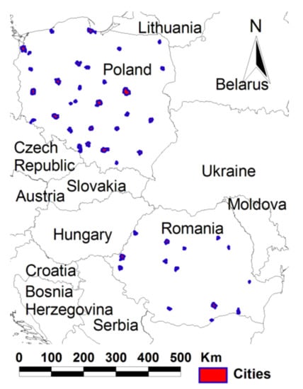
Figure 1.
Cities included in the study. The size of the cities was enlarged for a better visualization of their position.
Although the Urban Atlas was designed in theory to include cities with a population of over 100,000, in each country analyzed in this study smaller cities were included, and larger cities were left out. This was a shortcoming of the data, and could not be addressed by the current study, which had to use the available data. Although newer versions of the Urban Atlas included cities corresponding to the criteria, we could not include them due to the data missing from the earlier periods.
It must be stressed that the Urban Atlas data covered more than the city, i.e., its Functional Urban Area (FUA), defined as a contiguous set of municipalities which had at least 50% of their population in the urban center (defined as the contiguous set of urban cells of 1 km by 1 km with a population density of at least 1500 inhabitants/km2 and a total population of at least 50,000 inhabitants), plus the surrounding municipalities for which at least 15% of the employed persons commuted to the main municipality of the urban agglomeration [44]. Although cities exerted an influence over their FUA, it was impossible to ascertain using the Urban Atlas data alone; if a change occurred outside of the city limits it was due to that city or the drivers pertaining to the local administrative unit (LAU) where it occurred. Provided that the FUA of a city does not coincide with its administrative boundaries, the resulting contours of the FUA may include only parts of other local administrative units (LAUs). This will make an objective assessment of the potential drivers almost impossible. The decision to include only a share of the data (population, etc.) pertaining to a given unit equal to its share from the FUA of the larger city is arbitrary. Hence, the only feasible solution is to use only that part of the FUA, which lies within the administrative limits of the Urban Atlas cities in the analyses.
Moreover, additional decisions had to be taken with respect to further processing the data. Firstly, since our study looked at the dynamics of OGA in relation to planning, we focused naturally on human-driven changes. The study by Petrisor et al. [8] showed that the Urban Atlas categories corresponding to GI were (a) agricultural and semi-natural areas and wetlands, (b) forests, (c) green areas, (d) sports and leisure areas, and (e) water bodies. However, this study addressed only OGA, and the analysis was limited to the following four classes: green urban areas, sports and leisure facilities, and all “agricultural” and “natural” lands.
Secondly, the 2006 dataset differed from those of 2012 and 2018 through its classification scheme. Hence, in 2006, “agricultural” and “natural” lands each formed a single class, while the 2012 and 2018 datasets split them into sub-categories. Using the raw data in the analysis would have affected the results, especially the indices related to the fragmentation and transformation of OGA, because a single plot of land from 2006 would appear split over the next periods, due to a fine-tuned classification and not to the interventions resulting from it. For this reason, we reclassified the 2012 and 2018 data, thereby matching the 2006 classification scheme. We also made sure that the land use change data did not include a transformation of the two 2006 unique categories into sub-categories as “change”, or the conversion of a sub-category into another during 2012–2018.
2.1.1. Mathematical Model of Fragmentation
Some exceptions notwithstanding, the shape of most European cities is roughly circular, thereby strongly indicating the presence of a core-periphery structure [45,46]. Hence, if fragmentation is modeled by the ‘breaking of a mirror’ approach, the same initial area is divided into smaller areas, thus increasing the total perimeter through what is known as the ‘edge effect’.
Against this background, Rutledge [47] compared several indices of fragmentation, showing both their advantages and disadvantages. The findings indicated that a good index was invariant to the size of the study area, but accounted for its geometry instead. Fractal measures had this advantage, but the study by Petrisor et al. [8] showed that a fractal analysis yielded more than one index describing the fragmentation process, thus making the overall interpretation difficult, due to the individual variations across the indices.
The mathematical proof below shows the derivation of the fragmentation index (F), starting from the following points:
- The ‘perimeter to area ratio’ mentioned by Rutledge [47], consisting of the ratio between the perimeter and the area, which is the most suited to the ‘broken mirror’ model, is 1 for a circle.
- Additionally, if the total area is constant, the fragmentation process increases its value with the total perimeter.
Proof.
For a circle with the radius r, the area is , and the perimeter is .
Following Rutledge [47], we can calculate F′, the perimeter-to-area ratio:
Hence, in order to assess whether a fragmentation process occurred, we considered the ratio of the fragmentation index in the final year and its value in the first year: FI = F2012/F2006, and FI = F2018/F2012. The fragmentation index (FI) was computed for the total area and perimeter of OGA within each city separately. □
2.1.2. Indices Assessing the Transformations of OGA
In this study, we reclassified the Urban Atlas data on land use changes by extracting only the categories of interest from the original datasets, and subsequently totalling them all up as ‘OGA’. We then derived the following indices describing the dynamics of OGA across the chosen FUAs, using the X-Tool extension of ArcView GIS 3.X (ESRI, Redlands, CA, USA):
- FI (fragmentation): the fragmentation index, as defined in Section 2.1.1.
- G (gain): the increase in the total area of OGA through the transformation of other land uses into one of the four categories of GI corresponding to OGA: green urban areas, sports and leisure facilities, “agricultural” and “natural” lands.
- L (loss): the decrease in the total area of OGA through the transformation of the four categories of GI corresponding to OGA in other land uses.
- B (balance): the difference between the two indices above (G–L). The dynamic can either be positive or negative.
- T (inner transformation): the transformation of one of the four categories of GI corresponding to OGA into another category, measuring the human pressure within the green areas.
2.1.3. Predictors
Independent variables used to explain the behavior of the five indices above consisted of collateral data on the factors that could, in principle, influence the dynamics of green urban infrastructure, collected for the two countries from statistical yearbooks. We therefore selected them based on the following criteria: (1) measuring possible drivers of change, as identified in the literature review; (2) consistency and computation in the same way for both countries; (3) the ability to represent economic or social phenomena, and (4) the availability in official sources (the Central Statistical Office of Poland and the National Statistical Institute in Romania) for all cities, both years, and both countries. A decision had to be made for the local budgets (revenues and expenditures), as data existed only in a local currency. Since the conversion of data in one currency or another or into euros distorted the comparisons, and the indicator used for the comparisons of the two periods (ratio of the budget during the end year and its correspondent for the beginning year) was irrespective of the currency used, we used the raw data.
2.2. Methodology
This study uses an “ecological approach” in the epidemiological sense of the term [48]: a study carried out at the population level instead of the individual one. We chose this particular design due to its limitations, as presented in the Discussion section, because the spatial data was available at the city level only. The analogy with epidemiological studies is continued by using rates instead of absolute (raw) values, in order to overcome the differences between cities and countries. The rates are more suitable for assessing the relationship between the dynamics of OGA, seen as a process, as well as the dynamics of its drivers, also seen as a process. As a consequence, we used ratios of the values in 2012 and 2006, as well as in 2018 and 2012, respectively. We preferred ratios to differences because they were positive, non-dimensional and invariant to city size. Consequently, the study used the variables presented in Table 3.
Table 3.
Variables included in the study and their definitions.
The study employed the following statistical methods:
- A study in the dynamics of the fragmentation index and the gain, loss, dynamic, and inner transformation of OGA was conducted in each city during the study period, in order to see whether the difference between the values from 2012 and 2006, and between 2018 and 2012, respectively, were positive or negative.
- ANCOVA analyses were used to look at the simultaneous influence of the set of independent variables on each dependent variable, for both the global data and for each country separately, specifically assessing the simultaneous dependence of the fragmentation index and the gain, loss, dynamic, and inner transformation of OGA on the predictors: built-up area of the city, population of the city, population density, number of building permits, number of new dwellings completed, number of employed people, and total length of roads.
- A correlation analysis (based on computing the Bravais-Pearson coefficient of the linear correlation and its significance, in Excel 2003) was used to test whether correlations exist between the components of each possible pair of dependent and independent variables: fragmentation index, raw gain (ha), raw loss (ha), raw dynamic (ha), raw transformation of OGA (ha), gain ratio, loss ratio, dynamic ratio, inner transformation of OGA ratio, population of the city (ratio), population density (ratio), number of building permits (ratio), number of new dwellings completed (ratio), number of employed people (ratio), total length of roads (ratio), total length of modernized road (ratio)s, local budget-revenues (ratio), and local budget expenses (ratio).
The statistical procedures were implemented using the programs R (R Core Team, Vienna, Austria) [49] with the packages “car” and “psych” [50,51] and Microsoft Excel 2003. The level of significance was 0.5 for all analyses.
3. Results
The present study was carried out in the cities represented in the Urban Atlas from 2006–2018; 32 cities in Poland, and 14 cities in Romania. The following results present an overall picture of the trends affecting OGA (fragmentation, gain, loss, overall balance, and inner transformation) in the studied cities, regardless of the values of the parameters. Additional details can be found in Table 4, and maps in Figure 2.
Table 4.
Trends of the changes of OGA in the Polish and Romanian cities during 2006–2018.
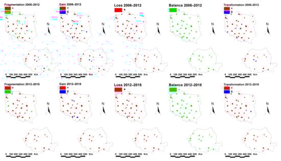
Figure 2.
Dynamic of the main indicators of OGA (fragmentation, gain, loss, overall balance and transformation) in Urban Atlas Polish and Romanian cities during 2006–2012 and 2012–2018. Green indicates positive values, meaning that fragmentation increased in intensity (images labeled “Fragmentation”), some OGA were gained (“Gain”), some OGA were lost (“Loss”), more OGA were gained than lost (images labeled “Balance”), and some OGA suffered inner changes (“Transformation”). Negative values (red) indicate the contrary, and blue shows no change. The size of the cities was enlarged for a better visualization of their position and dynamics of OGA.
- The fragmentation manifests itself differently in the two periods; the trend is less consistent from 2006–2012 (18/32 Polish and 11/14 Romanian cities), and stronger in the next period (29/32 Polish and 14/14 Romanian cities). The second period corresponds to the recovery after the economic crisis and a development boom.
- OGA were lost through the change to other uses in all cities from 2006–2012 and 2012–2018, as shown by the “Loss” indicator. Although new infrastructure was created through the transformation of other uses in some cities, as shown by the “Gain”, the overall 2006–2018 balance-indicated by the “Balance” showed that all of the cities permanently lost some OGA.
- OGA were subject to changes between 2006 and 2018 in many cities, especially from 2006–2012. These changes might pinpoint future land use changes.
- There were some cities that in one period, or both periods, showed no gain and/or transformation of OGA. Most likely, these local variations also depended on the resolution of data.
The results revealed some alarming trends, given the fact that the study was carried out in two countries with different planning practices and different social and economic dynamics: OGA continue to be fragmented in most cities, and lost in all cities.
Our statistical analysis aimed to check whether the variation in the area covered by OGA (fragmentation, gain, loss, overall balance, and inner transformation) could be explained by any of the socio-economic predictors, simultaneously or individually. The results of testing the simultaneous influence proved inconclusive. When looking at the raw values of the areas affected by changes of OGA, the global set of predictors showed no significant influence (at p = 0.05). When these values were expressed as a share of the city area, the global set of predictors had a significant influence, but very few predictors proved to exert a significant individual influence.
For this reason, the results of the correlation analysis, displayed in Table 5, are more relevant. The table displays the results for both countries taken together, as well as for Poland and for Romania separately. One might find a correlation between the raw gain and loss of OGA surprising; however, this is a typical case of confounding, where both indicators are related to the city size; more precisely, the larger the city, the larger the areas affected by the gain or loss of OGA. This is why the correlation is no longer present when the gain and loss are computed as a share of the urban area.
Table 5.
Correlation analysis of the variables describing the changes of OGA and possible predictors.
The results suggested that all the predictors could explain at least some of the phenomena affecting OGA. However, the overall findings were not necessarily applicable to each country separately, and differed from one period to another. Moreover, we were unable to identify a single driver responsible for all the transformations of OGA, even for a single period and country. While the small number of cities studied could be a potential explanation, this did not hold true in all cases. For example, in Romania, where the sample consisted of only 14 cities, the loss of OGA was found to correlate from 2012–2018 with the number of employees and local budgets (revenues and expenses); these correlations were not found in Poland or in the overall results during the same period. Similarly, in Poland and in the overall results, the number of employees was significantly correlated from 2006–2012 with the raw loss and balance of OGA; none of these correlations were found in Romania during the same period, although they were present from 2012–2018, when they were missing from Poland and the overall results.
4. Discussion
4.1. Significance of the Results
Our results showed that, regardless of the differences between the cities analyzed and between the two countries, in terms of the planning systems and socioeconomic dynamics during the study period, OGA were lost and fragmented in both Romanian and Polish cities between 2006 and 2018. Albeit alarming, this trend was consistent with other findings covering almost two decades [4,52]. Hence, the broader relevance of these findings is as follows:
- From a theoretical perspective, the results provided additional evidence verifying the hypothesis, often repeated in the literature, regarding the crucial impact of urbanization processes on the fragmentation of OGA in special and UGI in general.
- From a methodological perspective, the mathematical model of fragmentation, applicable to most European cities and potentially to any city with a concentric growth pattern, and invariant to the size of the city, proved its utility in bringing new and potentially different perspectives to the fragmentation process.
- This study resulted in concrete recommendations for planners (presented in Section 5). However, the main contribution of this article was the proof that, for the time being, these recommendations could be based solely on precautionary principles. Simply put, both the dedicated literature and the quality of the available datasets prevented us from making precise and mature recommendations for planning practitioners that were based on conclusive proofs. We believe this to be a major problem with current research practices, for reasons not sufficiently debated within the current literature.
- Additionally, last but not least, even though some studies that were carried out separately in different countries were are available in the existing literature, very few investigations were carried out in several countries simultaneously, especially in countries with different planning systems.
Returning to our key findings, the significance of the loss and fragmentation affecting OGA and UGI should be analyzed separately. Given the ES it provides (from a socioeconomic perspective) and its diversity (from an ecological standpoint), its loss can be seen as a negative phenomenon. However, its fragmentation can be placed in a “gray” area of the literature, especially within landscape ecology. When reviewing empirical studies carried out at the landscape scale, Fahrig [53] concluded that the ecological responses to habitat fragmentation per se (i.e., studies that were irrespective to the size of the habitat) were in most cases insignificant, while the most significant relationships were positive, as indicated by the increase in indicators such as species abundance, occurrence, richness, and other response variables to habitat fragmentation per se. This particular article drew upon an article making a contrary statement [54], followed by a new set of arguments provided by Fahrig et al. [55] supporting the claim that fragmentation was not “bad” per se. Since the present study did not deal directly with the ecological responses to the fragmentation, the only implication of the findings indicating the loss of UGI was a call for prudence, applying the precautionary principle.
Moreover, there are several local variations, especially related to the significance of drivers affecting the dynamics of OGA. An important limitation of this particular study lies in the fact that the statistical indicators differed from one country to another rather dramatically, ranging from measuring different indicators to measuring the same indicator in different ways. This is why the chosen set of indicators is confined to the common indicators, where by “common” we mean that they measure the same indicator in the same way.
Unfortunately, this explicit care did not always succeed in investigating some of the driving forces affecting the dynamics of OGA and UGI in depth. For example, in Romania data existed not only on the total length of roads in a given city, which usually showed little variation over time, but also on the modernization of roads, which could eventually result in the removal of adjacent vegetation rows. This indicator was identified as a significant driver for the fragmentation of OGA, for its loss, as well as for the overall balance, unlike the total length of roads. However, it could not be used in Poland, since it was computed in a different way. Similarly, unlike Poland, Romania did not have any indicators on the local Gross Domestic Product, and the only indicator for the overall state of the economy was employment. In summary, while the original plan was to check the influence of all the pillars of sustainability, except for the environmental ones, by selecting the most appropriate social, economic, and cultural indicators, we ended up with the indicators which permitted a comparison of both countries.
The different fragmentation trends, with several cities showing a constant compaction trend, must be correlated with the fact that the other results indicated a continuous loss of OGA. Against this background, we can easily infer that most of the small patches of OGA disappeared, and the remaining parts were found in untouchable areas (public parks and other types of green spaces). This explains both the compression and loss of OGA.
The vicious circle described by Petrişor et al. [8] was also valid for the relationship between climate changes, GI, and planning: a well-planned GI could help mitigate climate changes, but changes to GI due to the lack of or poor planning were likely to increase the negative outcomes of climate changes. If we considered that post-socialist countries were more vulnerable to climate change [56], this study made an important contribution to investigating the relationship between the effects of changing planning policies, particularly in the relationship with GI, and the ability to cope with the effects of climate change, strengthening the importance of addressing GI in planning, and helping to implement planning provisions addressing climate change issues.
4.2. Relevance of the Study Period
As mentioned above, the timeframe we investigated spanned the period between 2006 and 2018. However, our primary interest was in the period from 2006–2012, with the analyses from 2012–2018 conducted for inner validation purposes and for looking at the consistency of trends. In Romania, the period overlaps with the peak in the “real estate boom” occurring between 2006 and 2008, and the subsequent unfolding of the economic crisis between 2008 and 2012, both for the national economy in general and for the construction sector in particular. As a consequence, the values of different socio-economic indicators could be similar in the first and final year, with decreasing trends until 2012 followed by a growth continuing until 2018. The analyses could be run separately to account for the effects of the real estate boom and of the economic crisis, but unfortunately no data were available for the intermediary years. This suggested that the period of updating the Urban Atlas data should be shorter than six years, in order to account for finer-tuned studies, in line with real urban dynamics.
On the other hand, a “housing boom” occurred in Poland during the years 2008–2009. After this period, a slight decline was caused by the influence of the global crisis on the Polish economy. Although the impact of the crisis was definitely smaller than in other European countries and Poland was seen as a “green island” on the map of Europe, in the years from 2009–2011 there was a decrease in the number of completed apartments. Concomitantly, their usable floor area diminished and their price on the real estate market decreased [57]. After 2011, this trend became reversed, increasing continuously until 2018.
4.3. Similarities and Differences between Poland and Romania
The studies aimed to compare two European countries, situated in different parts of the continent (Poland in the center and Romania in the east). Both Poland and Romania as new members of the European Union, are rapidly developing countries. As part of the Eastern Bloc, they differed from other emerging economies in terms of their transition periods, a fact that could, in principle, be generalized to other emerging economies. The two countries developed rapidly in the 21st century, and although they shared some historical background, switched very quickly to their current developing paths. Hence, the study was relevant for countries with a similar background.
Previous studies showed that the urban sprawl in Europe was influenced by the historical structure of cities [23]. Furthermore, other studies pinpointed the influence of the planning system on integrating the concepts of GI and ES in the planning process [18,58].
Against this background, a simple look at the data reveals the differences between Polish and Romanian cities. Although their population does not differ significantly, the size of the Polish cities is significantly greater than that of the Romanian cities; roughly 2–3 times greater. Moreover, the share of OGA in Polish cities is significantly greater than in Romanian cities; roughly twofold. The local budget (revenues and expenditure) was significantly greater in the Polish cities from 2012–2018. Other differences were visible in the results we obtained: fragmentation was significantly greater in Romania from 2006–2012, and the overall balance, i.e., the difference between the area of gained and lost OGA, was greater in Poland during 2012–2018. Since the overall balance was a raw value, it could be explained by the significantly greater size of Polish cities.
Apart from these morphological differences, there were differences in the planning systems and in their dynamics as well. Although planning in general could play a key role in terms of enhancing OGA and maximizing their ES, there could also relevant differences between the Polish and Romanian planning systems.
The Polish planning system does not enforce, but instead stimulates the process of regulating different activities by plans. As a consequence, only a part of the administrative territory of the cities is covered by the plans. Since 2004, when the current law on spatial planning and development came into force, all spatial development plans adopted before 1 January 1995 lost their validity [59]. These legal regulations covered approximately 75% of the country’s area. This decision should be assessed very critically; it meant that many communes, and also urban municipalities, were left with no binding spatial plans. The plans were introduced despite the discontent and protests of self-government authorities [59]. As a result, some areas, previously protected by the provisions of spatial development plans, lost their primary protection.
In Romania, the planning system changed, but the planning process remained a long and arduous bureaucratic process [60]. The law required the existence of different plans, from the Master Plan of an entire city, or what is called a General Urban Plan in Romanian planning parlance, to a detailed plan for each planning objective or investment [60]. During the real estate boom, “derogatory planning” (i.e., legalizing deviations from the initial plan) accounted for most real estate developments [61]. After 2008, the planning became affected by economic crisis, while the period before 2008 corresponded to changes in the planning system as a consequence of the accession of Romania to the European Union [62]. As a consequence of changes in both periods, the plans at different spatial levels contradict each other [62] and the built reality is markedly different from planned intentions [63]. Furthermore, plans were drafted according to an outdated methodology, which lost connection with the progress of urban ecology [64] and did not account for key concepts, such as GI and its ES, allowing for its fragmentation without understanding the importance of continuity for its normal functioning, and ultimately for the welfare and comfort of the urban population [8].
An illustration might prove beneficial at this particular point. In Romania, each urban planning document follows a relatively similar development path. First, a design brief, with its associated terms of reference, is produced, either by a planning authority or by a team of consultants, hired for this task by the planning authority. Then, after a contract is signed, with the brief and the terms of reference as annexed to the contract, the drafting of the planning document commences.
The drafting process comprises four distinct stages: Firstly, a series of background studies are produced, which aim to support the proposals contained within the future planning document. Secondly, a preliminary version of the planning document is drafted by the design team. “Preliminary” in this sense means that the planning document is a development of an urban planning perspective. Once endorsed by the relevant local Technical Committee for Spatial and Urban Planning, which oversees urban development and acts in all major Romanian cities, the planning document enters its third stage, namely the application for notices and agreements from the relevant authorities. It is within this third stage that the planning document might suffer additional changes in order to correspond to various technical and legal requirements. After the successful completion of this third stage, the planning document is now in its final version, and can therefore be approved by the Architect in Chief, with the support of the same Technical Committee for Spatial and Urban Planning that we mentioned earlier. Once approved, it then enters its fifth and final stage, namely the endorsement by the Municipal Council.
It is plain to see that the pivotal component in this entire procedure is the quality of the design brief and of its associated terms of reference, which, as discussed earlier, become mandatory provisions through the inclusion in the contract. Now, the crux of the matter is that most Romanian design briefs, but not all, fare extremely poorly when assessed from a scientific perspective. The provisions related to GI are either completely absent, or else they are surprisingly weak, expressed in terms that became obsolete decades ago. Furthermore, the overwhelming majority of design briefs bow to the recommendations made by outdated technical guidelines, which have not been updated for over two decades. To complicate things further, even if newer-generation design briefs stand to correct this unfortunate state of affairs, they usually run the risk of being contested by potential bidders during the public procurement process.
Returning to our main argument, derogatory planning usually results in detailed plans which violate the provisions of General Urban Plans and oppose the initial planning goals [62] in order to legalize the developments occurring under political or economic pressure. Moreover, the legal requirement of updating the General Urban Plan every 5 to 10 years is not enforced with bureaucratic procedures resulting, under politically unstable conditions, in missed deadlines. At the three points in our study period (2006, 2012, and 2018), some cities did not have an updated plan with the validity of the previous plan being somewhat developed, or with a new plan drafted but not legally approved.
In contrast, the current spatial planning system in Poland was built up under political transformation conditions and based on the axiological assumption according to which the right to protect real property ownership could be extended to the right of land development. This meant that every property owner, by virtue of the act itself, had the right to develop it [59].
This right can be limited (forfeited) when pursuant to the current provisions, i.e., the local spatial development plan (or local plan). Its provisions cannot breach the arrangements of the document which determines the spatial policy of a certain commune, i.e., the study of determinants and directions of spatial development (called ‘study’). This study is a mandatory document, drawn up for the area of an entire commune, but it is not generally binding; therefore, no administrative decision can be based on it [65,66].
Unlike the study, local plans are not mandatory and only some parts of a commune can be included. Such plans are usually prepared for building-free areas (agricultural), stimulating the excessive development of urban areas over adjacent territories. Nevertheless, vast areas of cities and communes (municipalities) are not included in the plans; this does not mean there is no possibility of investing there. The administrative decisions on building conditions can still be applied in the areas not covered by plans. These decisions do not need to be compatible with the study and allow building development in areas with no technical infrastructure.
It is worth noting that, in the case of issuing building conditions, an investor, and not a commune, makes decisions on the land designation. Such a liberal law results in the fact that the construction industry can develop in an unplanned way in places preferred by investors, including floodplains, areas with significant landscapes and environmental assets, etc. This results in a decreasing in the functional efficiency of cities and their capacities for effective and sustainable development, deteriorating the quality of the natural environment and increasing the pressure on building-free areas (including the green areas). The adopted planning solutions refer, to a small extent, to the basic spatial planning principles, which ensure spatial order and sustainable development in Poland. Because of this, the Polish spatial planning system is widely criticized in the literature [59,65,66]. Its weaknesses are proven, among others, by the results of the study conducted in selected Polish cities by the Supreme Audit Office in 2017; they show that, despite the expansion of the area covered by local plans, many cities recorded a decrease in the share of green areas and water in the total area structure included in the local plans [67].
Against this background, Table 6 presents a comparison between the studied cities in the country-specific planning context: the existence and updating with plans in Romania, and the share of the city area covered by plans in Poland. The latest decreases during some periods and in some cities (2006–2012 in Gdańsk, 2012–2018 in Opole and Zielona Góra) are explained by the fact that the city area increased and the existing plans covered a smaller part of it.
Table 6.
Planning status of the studied cities, according to the different planning systems in each country: existence of an up-to-date plan in Romania and share of the planned area from the city area in Poland.
In summary, the lack of coverage by plans in Poland and the derogatory over-planning in Romania had the same effect: development occurred spontaneously, driven by economic and political forces, and did not account for GI, which were fragmented and lost in both countries.
4.4. Study Design
The study employed an ecological approach, which is, by design, subject to the “ecological fallacy”, meaning that the conclusions obtained at the population level are generally not valid at the individual level [68] due to spurious correlations. For instance, a country-wide analysis indicates that the loss of OGA, measured by the difference in area between 2006 and 2012 or 2012 and 2018, is significantly greater in Poland than in Romania, simply because Polish cities are larger than their Romanian counterparts. If the loss is measured as a ratio between the difference in area and city size in 2006 and 2012, or 2012 and 2018, the difference is no longer significant. Furthermore, the ecological fallacy relates to confounding, when variables which are not functionally related appear to be correlated because both are tied to the same third variable. This confounding of results causes a spurious correlation between the raw gain and loss of OGA, both related to city size. Regardless of its inherent shortcomings, the ecological approach has the theoretical advantage of allowing the simultaneous comparison of large amounts of information; therefore, 46 cities are analyzed in the study, with the caveat of relying mostly on quantitative data and treating event qualitative data in a quantitative manner, i.e., integrating it the ANCOVA prediction model. In addition to this, the validity of the approach is proven by its use in studies from other fields, including management, health, sociology, geography, or political studies, to name only a few [69,70,71,72,73].
The ANCOVA prediction model is also subject to limitations: We already pointed out the issue of data availability at the city level, which resulted in a lesser coverage of the economic and social aspects of sustainability. Nevertheless, with this caveat in mind, the model has the theoretical advantage of being able to address the traditional pillars of sustainability (economy, society, and environment), but also some additional dimensions of the concept, i.e., infrastructure, demography, and administration. In addition, its validity results from totaling predictors found to be significant for the dynamics of GI by other studies.
Although the mathematical model used in this study is a novel approach, the findings are consistent with those of previous studies, thereby validating it implicitly, in addition to its mathematical proof. However, the main limitation of this model is that it relies on the radial-concentric geometry of cities. Further research is needed to derive similar models for other shapes, keeping in mind that its development starts from the condition of creating a model that is invariant to the original size of the initial city shape.
4.5. Data and Methodological Limitations, and Future Research Directions
Due to the nature of the data, we deliberately and justifiably assumed several limitations for this study. It must be pointed out that, despite the free availability of European geospatial data such as CORINE or the Urban Atlas, datasets are continuously subject to changes intended to improve them, both in terms of resolution and classification schemes. However, these changes also entail important limitations, with the difficulty of conducting comparative analyses being chief among them [74]. In our case, the different classification scheme used in 2006 compared to 2012 and 2018 was overcome by reclassifying the newer datasets, thereby diminishing their resolution. Future research using newer data would naturally benefit from a more complex classification scheme, but analyses aimed at searching an entire period will have to deal with this issue for the 2006 data.
At the same time, we decided to limit our analyses to GI corresponding to OGA. Future studies could also take into account GI and even “blue-green infrastructure”, since the data are already available. Nevertheless, the inability of discerning between changes in infrastructure which are due to human interventions or have different underlying causes still remains.
Last but not least, for comparison purposes the analysis was limited to the cities covered by Urban Atlas data in all the three periods analyzed, while statistical analyses were carried out only for those cities where data on the different drivers was available. This was another limitation likely to affect the future studies, since the data could not be produced retroactively. While the limitation is inherent to the data and cannot be addressed, future studies could focus on the more recent periods, provided that the data include more cities. At the same time, future studies focusing on recent data will benefit from using larger samples and cities that might be more relevant for statistical purposes (for instance, large Romanian cities, such as Iași, Brașov, Constanța, or Galați, meeting the population criterion, were not included in the analysis due to the lack of available data for 2006).
In methodological terms, the characteristics of the study team allowed for a simple and intuitive spatial analysis, able to translate the spatial data into numbers that could be analyzed statistically, task accomplished using ArcView GIS 3.X. Future studies could consider using more recent pieces of software, such as QGIS and its Phyton language script, which are able not only to collect data, but also to pinpoint the most and least correlated areas, allowing for the involvement of “a broader audience” and a better visualization of the final output, tools that ultimately improve the decision-making process.
In conceptual terms, our study was strictly focused on the dynamic of OGA in relationship to the drivers influencing it and the planning perspective. However, moving to the landscape scale, there were other issues worth exploring, such as the effects generated by urban transformations on landscape, their relationships with ecological connectivity, and the economic attractiveness that may be generated in a city or territory [75,76], or the relationship with the global resilience, in particular to climate change.
Against this background, we can now sum up the main limitations of this study. Hence, we know that all FUAs under scrutiny lost OGA over the period between 2006 and 2018. However, we do not know precisely which kind of GI were lost. Additionally, perhaps even more importantly, we can only formulate recommendations based on precautionary principles, given the quality of the available data.
Each of the previous statements requires a brief explanation. Hence, as mentioned earlier, FUAs encompass more than one municipality. Moreover, FUA boundaries do not always overlap administrative boundaries, which are the main units for census data. Therefore, we cannot confirm a FUA-wide analysis by using additional, finer-grained examinations, aimed at probing the real situation of GI within the administrative boundaries of the constituent municipalities. This is a problem, especially when most of the green open spaces within any given FUA are located across its periphery, and not within its core. Consequently, when we talk about losing GI, we usually mean losing GI at the fringes of the FUA, generally due to the urban sprawl generated by its core. Moreover, this infrastructure consists mostly of agricultural and natural areas, with urban green open spaces or leisure areas being far less common. However, the lack of overlap between FUA and administrative boundaries prevents us from pinpointing the exact amount and position of the lost GI in relation to each municipality’s administrative boundaries. Therefore, we can only say that FUAs lose OGA, most likely at their fringes, where the urban sprawl generated by the core transforms green open spaces into built-up areas. At the same time, better planning recommendations can be phrased through the lens of the four types of urban nature; if the city growth the likely to eliminate and fragment natural areas with their biodiversity, planners can provide for landscaped areas connecting remaining natural islands and ensuring the provision of ES, compensating for the lost ones. In this regard, studies using a fine-grained classification of different types of GI can provide more specific recommendations.
Secondly, it is very important to stress that satellite imagery tells us very little about land use, and, even more importantly, about development rights enshrined within the legal status of each plot. Hence, the administrative anatomy of an FUA is further complicated by the fact that each constituent municipality is governed at least by one urban plan, i.e., the general urban plan for the entire municipality, or a series of zonal urban plans, for different areas within that municipality. It is these plans that affect development rights and might consequently distort the interpretation of satellite imagery. In other words, plots which have not yet been built or that still lie derelict, even if construction is legally possible, might be covered by greenery, and thus appear as part of GI. Moreover, there is a fine line when classifying wooded areas as “forests”, based on the canopy coverage and depending on the spatial resolution of the image. In other words, only large developments may be classified as “change”, while small transformations cannot always be detected.
It is against this background that we can only formulate recommendations based on precautionary principles, because of the gaps in the scientific literature and quality and availability of the data. This is a crucial point to be made, as our recommendations eventually filter through to planning regulations, which are opposable in a court of law [77].
5. Conclusions and Recommendations
The present study was aimed at answering three questions related to the variables that could help predict the dynamics of OGA, the relationship between the differences in the dynamics of OGA in the two countries, and the insights for planning practitioners. With respect to the first two questions, our findings indicated that OGA continued to be fragmented in most cities, and lost in all cities. The drivers included urban built-up areas, population and density, the number of building permits, number of new dwellings completed, number of employees, and the total length of roads. However, the overall findings did not necessarily apply to each country separately and differed from one period to another. Moreover, a single driver cannot be held responsible for all the transformations of GI, even for a single period and country. Despite the different planning systems, the lack of coverage by plans in Poland and the derogatory over-planning in Romania had the same effect: development occurred spontaneously, driven by economic and political forces and did not account for OGA, which were fragmented and lost in both countries.
In a nutshell, the key message of the study is the following: Regardless of the planning systems of the two countries, this study shows that OGA continue to be fragmented and lost. Therefore, the scope of studies is expanded demonstrating this decline. Unfortunately, there is a lack of proactive regulations and instruments for stopping the process, as well as clear-cut guidelines for accomplishing this task. Furthermore, the existing planning literature does not succeed in providing clear and convincing arguments that justify the need for such tools.
It is against this background that we can now make a series of operational recommendation to planners:
- Since design briefs and their associated terms of reference gain contractual power through their inclusion in the public procurement contracts for urban planning documents, they need to have a thorough scientific grounding, as well as a critical perspective on current research. This point cannot be stressed explicitly enough, as a lot of academic output on ES and planning practices in general is surprisingly shallow. It is within such a context that design briefs and their associated terms of reference have the capacity to act as the main drivers for the improvement of future planning documents. Therefore, we strongly urge planning authorities and their consultants to carefully and critically peruse the available scientific literature on ES and to introduce dedicated background studies with expected sets of results in each design brief dedicated to complex urban documents.
- Furthermore, we urge the academic community to try harder and to study the planning process in greater depth, as many of their recommendations are divorced from the planning reality. Recommendations need to be mature enough to be operational, otherwise they are useless to even the most well-disposed of planning practitioners. As we saw earlier while conducting the literature review, academic output was almost entirely self-sufficient, with no real desire to bridge the gap between academia and planning practices. Needless to say, in an ever-changing legal and normative context, operational knowledge is crucial for planners.
- Additionally, last but not least, we encourage academics to produce scientifically informed design manuals, which then can be put to the test in the real world.
Author Contributions
All the authors equally contributed to the article. Conceptualization, A.-I.P., L.M., A.M. and K.D.; methodology, A.-I.P., L.M., A.M. and K.D.; formal analysis, A.-I.P., L.M., A.M. and K.D.; investigation, A.-I.P., L.M., A.M., K.D. and A.V.T.; resources, A.-I.P., L.M., A.M., K.D. and A.V.T.; data curation, A.-I.P., L.M., A.M., K.D. and A.V.T.; writing—original draft preparation, A.-I.P., L.M., A.M. and K.D.; writing—review and editing, A.-I.P., L.M., A.M. and K.D.; validation, A.-I.P., L.M., A.M. and K.D.; visualization, A.-I.P., L.M., A.M. and K.D.; software, K.D. and A.V.T.; supervision, A.-I.P.; project administration, A.-I.P. All authors have read and agreed to the published version of the manuscript.
Funding
This research received no external funding.
Institutional Review Board Statement
Not applicable.
Informed Consent Statement
Not applicable.
Data Availability Statement
This study used existing data. Processed data cannot be easily stored due to the size, but can be obtained by demand from the corresponding author.
Conflicts of Interest
The authors declare no conflict of interest.
References
- Cohen, J.E. Human population: The next half century. Science 2003, 302, 1172–1175. [Google Scholar] [CrossRef]
- Grimm, N.B.; Faeth, S.H.; Golubiewski, N.E.; Redman, C.L.; Wu, J.; Bai, X.; Briggs, J.M. Global Change and the Ecology of Cities. Science 2008, 319, 756–760. [Google Scholar] [CrossRef] [Green Version]
- Wu, J. Urban ecology and sustainability: The state-of-the-science and future directions. Landsc. Urban Plan. 2014, 125, 209–221. [Google Scholar] [CrossRef]
- Tzoulas, K.; Korpela, K.; Venn, S.; Yli-Pelkonen, V.; Kazmierczak, A.; Niemelä, J.; James, P. Promoting Ecosystem and Human Health in Urban Areas using Green Infrastructure: A Literature Review. Landsc. Urban Plan. 2007, 81, 167–178. [Google Scholar] [CrossRef] [Green Version]
- Mell, I.C. Green Infrastructure: Concepts and planning. Newctle. Univ. Forum Ej. 2008, 8, 69–80. [Google Scholar]
- Cilliers, S.; Cilliers, J.; Lubbe, R.; Siebert, S. Ecosystem services of urban green spaces in African countries—Perspectives and challenges. Urban Ecosyst. 2013, 16, 681–702. [Google Scholar] [CrossRef]
- Gómez-Baggethun, E.; Gren, Å.; Barton, D.N.; Langemeyer, J.; McPhearson, T.; O’Farrell, P.; Andersson, E.; Hamstead, Z.; Kremer, P. Urban Ecosystem Services. In Urbanization, Biodiversity and Ecosystem Services: Challenges and Opportunities. A Global Assessment; Elmqvist, T., Fragkias, M., Goodness, J., Güneralp, B., Marcotullio, P.J., McDonald, R.I., Parnell, S., Schewenius, M., Sendstad, M., Seto, K.C., et al., Eds.; Springer: Berlin, Germany, 2013; pp. 175–251. [Google Scholar]
- Petrişor, A.-I.; Andronache, I.C.; Petrişor, L.E.; Ciobotaru, A.-M.; Peptenatu, D. Assessing the fragmentation of the green infrastructure in Romanian cities using fractal models and numerical taxonomy. Proc. Env. Sci. 2016, 32, 110–123. [Google Scholar] [CrossRef] [Green Version]
- Zwierzchowska, I.; Hof, A.; Ioja, I.C.; Mueller, C.; Ponizy, L.; Breuste, J.H.; Mizgajski, A. Multi-Scale Assessment of Cultural Ecosystem Services of Parks in Central European Cities. Urban For. Urban Green. 2018, 30, 84–97. [Google Scholar] [CrossRef]
- Melles, S.; Glenn, S.; Martin, K. Urban bird diversity and landscape complexity: Species—Environment associations along a multiscale habitat gradient. Ecol. Soc. 2003, 7, 5. [Google Scholar] [CrossRef] [Green Version]
- Niemelä, J.; Saarela, S.-R.; Söderman, T.; Kopperoinen, L.; Yli-Pelkonen, V.; Väre, S.; Kotze, D.J. Using the ecosystem services approach for better planning and conservation of urban green spaces: A Finland case study. Biodivers. Conserv. 2010, 19, 3225–3243. [Google Scholar] [CrossRef]
- Niemelä, J. Ecology and urban planning. Biodivers. Conserv. 1999, 8, 119–131. [Google Scholar] [CrossRef]
- Fernández-Juricic, E.; Jokimäki, J. A habitat island approach to conserving birds in urban landscapes: Case studies from southern and northern Europe. Biodivers. Conserv. 2001, 10, 2023–2043. [Google Scholar] [CrossRef]
- Pauleit, S.; Ennos, R.; Golding, Y. Modeling the environmental impacts of urban land use and land cover change—A study in Merseyside, UK. Landsc. Urban Plan. 2005, 71, 295–310. [Google Scholar] [CrossRef]
- Angold, P.G.; Sadler, J.P.; Hill, M.O.; Pullin, A.; Rushton, S.; Austin, K.C.; Small, E.; Wood, B.C.; Wadsworth, R.; Sanderson, R.A.; et al. Biodiversity in urban habitat patches. Sci. Total Environ. 2006, 360, 196–204. [Google Scholar] [CrossRef]
- Young, R.F. Managing municipal green space for ecosystem services. Urban For. Urban Green. 2010, 9, 313–321. [Google Scholar] [CrossRef]
- Clergeau, P.; Linglart, M.; Morin, S.; Paris, M.; Dangeon, M. La trame verte et bleue à l’épreuve de la ville (The green and blue corridors working for the city). Trait. Urbains 2016, 83, 37–40. [Google Scholar]
- Artmann, M.; Bastian, O.; Grunewald, K. Using the Concepts of Green Infrastructure and Ecosystem Services to Specify Leitbilder for Compact and Green Cities—The Example of the Landscape Plan of Dresden (Germany). Sustainability 2017, 9, 198. [Google Scholar] [CrossRef] [Green Version]
- Razin, E.; Rosentraub, M. Are Fragmentation and Sprawl Interlinked? North American Evidence. Urban Aff. Rev. 2000, 35, 821–835. [Google Scholar] [CrossRef]
- Gibb, H.; Hochuli, D.F. Habitat fragmentation in an urban environment: Large and small fragments support different arthropod assemblages. Biol. Conserv. 2002, 106, 91–100. [Google Scholar] [CrossRef]
- Luck, M.; Wu, J. A gradient analysis of urban landscape pattern: A case study from the Phoenix metropolitan region, Arizona, USA. Landsc. Ecol. 2002, 17, 327–339. [Google Scholar] [CrossRef]
- McKinney, M.L. Effects of urbanization on species richness: A review of plants and animals. Urban Ecosyst. 2008, 11, 161–176. [Google Scholar] [CrossRef]
- Poelmans, L.; Van Rompaey, A. Detecting and modelling spatial patterns of urban sprawl in highly fragmented areas: A case study in the Flanders-Brussels region. Landsc. Urban Plan. 2009, 93, 10–19. [Google Scholar] [CrossRef]
- Andersson, E.; Barthel, S.; Borgström, S.; Colding, J.; Elmqvist, T.; Folke, C.; Gren, Å. Reconnecting Cities to the Biosphere: Stewardship of Green Infrastructure and Urban Ecosystem Services. Ambio 2014, 43, 445–453. [Google Scholar] [CrossRef] [Green Version]
- EC. Green Infrastructure (GI)—Enhancing Europe’s Natural Capital; EC: Brussels, Belgium, 2013. [Google Scholar]
- Qureshi, S.; Breuste, J.H. Prospects of Biodiversity in the Mega-City of Karachi, Pakistan: Potentials, Constraints and Implications. In Urban Biodiversity and Design, 1st ed.; Müller, N., Werner, P., Kelcey, J.G., Eds.; Blackwell: Chichister, UK, 2010; pp. 497–517. [Google Scholar]
- Breuste, J.H.; Qureshi, S.; Li, J. Scaling down the ecosystem services at local level for urban parks of three megacities. Hercynia N. F. 2013, 46, 1–20. [Google Scholar]
- Ghofrani, Z.; Sposito, V.; Faggian, R. A Comprehensive Review of Blue-Green Infrastructure Concepts. Int. J. Environ. Sustain. 2017, 6, 15–36. [Google Scholar] [CrossRef]
- Sanesi, G.; Colangelo, G.; Lafortezza, R.; Calvo, E.; Davies, C. Urban green infrastructure and urban forests: A case study of the Metropolitan Area of Milan. Landsc. Res. 2017, 42, 164–175. [Google Scholar] [CrossRef]
- Dale, V.H.; Efroymnson, R.A.; Kline, K.L. The land use—Climate change—Energy nexus. Landsc. Ecol. 2011, 26, 755–773. [Google Scholar] [CrossRef]
- MEA. Millennium Ecosystem Assessment. Ecosystems and Human Well-Being: Synthesis; Island Press: Washington, DC, USA, 2005. [Google Scholar]
- UN. Transforming Our World: The 2030 Agenda for Sustainable Development; UN: New York, NY, USA, 2015; Available online: https://www.un.org/ga/search/view_doc.asp?symbol=A/%20RES/70/1=E (accessed on 27 September 2021).
- The Habitats Directive. The Habitats Directive Establishing Natura 2000 and Requiring Member States to Designate Special Areas of Conservation (SACs); The Habitats Directive: Brussels, Belgium, 1992. [Google Scholar]
- European Commission. Recovery Plan for Europe; European Commission: Brussels, Belgium, 2021; Available online: https://ec.europa.eu/info/strategy/recovery-plan-europe_en (accessed on 27 September 2021).
- Ojima, D.S.; Galvin, K.A.; Turner, B.L., II. The Global Impact of Land-Cover Change. BioScience 1994, 44, 300–304. [Google Scholar] [CrossRef]
- Lambin, E.F.; Rounsevell, M.D.A.; Geist, H.J. Are agricultural land-use models able to predict changes in land-use intensity? Agric. Ecosys. Environ. 2000, 82, 321–331. [Google Scholar] [CrossRef]
- Petrişor, A.-I. Using CORINE data to look at deforestation in Romania: Distribution & possible consequences. Urban Arhit. Constr. 2015, 6, 83–90. [Google Scholar]
- Pielke, R.A.; Marland, G.; Betts, R.A.; Chase, T.N.; Eastman, J.L.; Niles, J.O.; Running, S.W. The influence of land-use change and landscape dynamics on the climate system: Relevance to climate-change policy beyond the radiative effect of greenhouse gases. Philos. Trans. R. Soc. A 2002, 360, 1705–1719. [Google Scholar] [CrossRef] [PubMed]
- Xiao, J.; Shen, Y.; Ge, J.; Tateishia, R.; Tang, C.; Liang, Y.; Huang, Z. Evaluating urban expansion and land use change in Shijiazhuang, China, by using GIS and remote sensing. Landsc. Urban Plan. 2006, 75, 69–80. [Google Scholar] [CrossRef]
- Gill, S.E.; Handley, J.F.; Ennos, A.R.; Pauleit, S. Adapting Cities for Climate Change: The Role of the Green Infrastructure. Built Environ. 2007, 3, 115–133. [Google Scholar] [CrossRef] [Green Version]
- La Greca, P.; La Rosa, D.; Martinico, F.; Privitera, R. Agricultural and green infrastructures: The role of non-urbanised areas for eco-sustainable planning in a metropolitan region. Environ. Pollut. 2011, 159, 2193–2202. [Google Scholar] [CrossRef] [PubMed]
- Hagenauer, J.; Helbich, M. Mining urban land-use patterns from volunteered geographic information by means of genetic algorithms and artificial neural networks. Int. J. Geogr. Inf. Sci. 2012, 26, 963–982. [Google Scholar] [CrossRef]
- Prastacos, P.; Chrysoulakis, N.; Kochilakis, G. Spatial metrics for Greek cities using land cover information from the Urban Atlas. In Multidisciplinary Research on Geographical Information in Europe and Beyond. Proceedings of the AGILE’2012 International Conference on Geographic Information Science “Bridging the Geographic Information Science”, Avignon, France, 24–27 April 2012; Gensel, J., Josselin, D., Vandenbroucke, D., Eds.; Springer: Berlin, Germany, 2012; pp. 261–266. [Google Scholar]
- Dijkstra, L.; Poelman, H. Cities in Europe—The New OECD-EC Definition. Regional Focus 2012, RF1. Available online: http://ec.europa.eu/regional_policy/sources/docgener/focus/2012_01_city.pdf (accessed on 5 April 2021).
- Pénzes, J. The dimensions of peripheral areas and their restructuring in Central Europe. Hung. Geogr. Bull. 2013, 62, 373–386. [Google Scholar]
- Bardzinska-Bonenberg, T. Ring-and-circle, symbolical and practical meaning of the form in town planning and architecture. A: Virtual City and Territory. In Back to the Sense of the City: International Monograph Book; Cladera, J.R., Ed.; Centre de Política de Sòl i Valoracions: Barcelona, Spain, 2016; pp. 37–49. [Google Scholar]
- Rutledge, D. Landscape Indices as Measures of the Effects of Fragmentation: Can Pattern Reflect Process? DOC Science Internal Series No. 98; Department of Conservation: Wellington, New Zealand, 2003; pp. 1–27. [Google Scholar]
- Morgenstern, H. Ecologic studies in epidemiology: Concepts, principles, and methods. Annu. Rev. Public Health 1995, 16, 61–81. [Google Scholar] [CrossRef]
- R Core Team. R: A Language and Environment for Statistical Computing; R Foundation for Statistical Computing: Vienna, Austria; Available online: https://www.R-project.org (accessed on 2 July 2019).
- Fox, J.; Weisberg, S.; Price, B. Car: Companion to Applied Regression. Available online: https://CRAN.R-project.org/package=car (accessed on 2 July 2019).
- Revelle, W. Psych: Procedures for Psychological, Psychometric, and Personality Research. Available online: https://CRAN.R-project.org/package=psych (accessed on 2 July 2019).
- Kabisch, N.; Haase, D. Green spaces of European cities revisited for 1990–2006. Landsc. Urban Plan. 2013, 110, 113–122. [Google Scholar] [CrossRef]
- Fahrig, L. Ecological Responses to Habitat Fragmentation Per Se. Annu. Rev. Ecol. Evol. Syst. 2017, 48, 1–23. [Google Scholar] [CrossRef]
- Fletcher, R.J.; Didham, R.K.; Banks-Leite, C.; Barlow, J.; Ewers, R.M.; Rosindell, J.; Holt, R.D.; Gonzalez, A.; Pardini, R.; Damschen, E.I.; et al. Is habitat fragmentation good for biodiversity? Biol. Cons. 2018, 226, 9–15. [Google Scholar] [CrossRef] [Green Version]
- Fahrig, L.; Arroyo-Rodríguez, V.; Bennett, J.R.; Boucher-Lalonde, V.; Cazetta, E.; Currie, D.J.; Eigenbrod, F.; Ford, A.T.; Harrison, S.P.; Jaeger, J.A.G.; et al. Is habitat fragmentation bad for biodiversity? Biol. Cons. 2019, 230, 179–186. [Google Scholar] [CrossRef] [Green Version]
- Björnsen, G.A.; Bokwa, A.; Chełmicki, W.; Elbakidze, M.; Hirschmugl, M.; Hostert, P.; Ibisch, P.; Kozak, J.; Kuemmerle, T.; Matei, E.; et al. Global Change Research in the Carpathian Mountain Region. Mountain Res. Dev. 2009, 29, 282–288. [Google Scholar]
- Zaniewska, H.; Dąbkowski, N. Budownictwo mieszkaniowe w Polsce i jego standardy w latach 1991–2011 (Housing construction in Poland and its standards in the years 1991–2011). Probl. Rozw. Miast 2013, 10, 123–134. [Google Scholar]
- Badiu, D.-L.; Iojă, I.C.; Pătroescu, M.; Breuste, J.H.; Artmann, M.; Niţă, M.R.; Grădinaru, S.R.; Hossu, C.A.; Onose, D.-A. Is urban green space per capita a valuable target to achieve cities’ sustainability goals? Romania as a case study. Ecol. Ind. 2016, 70, 53–66. [Google Scholar] [CrossRef]
- Kolipiński, B. Planowanie przestrzenne w Polsce w minionym 25-leciu (Spatial planning in Poland in the last 25 years). Maz. Studia Reg. 2014, 15, 109–118. [Google Scholar]
- Petrişor, A.-I. The theory and practice of urban and spatial planning in Romania: Education, laws, actors, procedures, documents, plans, and spatial organization. A multiscale analysis. Serb. Arch. J. 2010, 2, 139–154. [Google Scholar] [CrossRef]
- Petrişor, A.-I.; Hamma, W.; Nguyen, H.D.; Randazzo, G.; Muzirafuti, A.; Stan, M.-I.; Tran, V.T.; Aştefănoaiei, R.; Bui, Q.-T.; Vintilă, D.-F.; et al. Degradation of Coastlines under the Pressure of Urbanization and Tourism: Evidence on the Change of Land Systems from Europe, Asia and Africa. Land 2020, 9, 275. [Google Scholar] [CrossRef]
- Munteanu, M.; Servillo, L. Romanian spatial planning system: Post-communist dynamics of change and Europeanization processes. Eur. Plan Stud. 2013, 22, 2248–2267. [Google Scholar] [CrossRef] [Green Version]
- Grădinaru, S.R.; Iojă, I.C.; Pătru-Stupariu, I.; Hersperger, A.M. Are spatial planning objectives reflected in the evolution of urban landscape patterns? A framework for the evaluation of spatial planning outcomes. Sustainability 2017, 9, 1279. [Google Scholar] [CrossRef] [Green Version]
- Petrişor, A.-I.; Petrişor, L.E. The shifting relationship between urban and spatial planning and the protection of the environment: Romania as a case study. Present Environ. Sustain. Dev. 2013, 7, 267–277. [Google Scholar]
- Mierzejewska, L. Urban planning in Poland in the context of European standards. Quaest. Geogr. 2009, 28, 29–38. [Google Scholar]
- Mierzejewska, L. Wybrane problemy planowania i zagospodarowania przestrzennego w miastach na prawach powiatu w Polsce (Selected issues of spatial planning and development in cities with poviat rights in Poland). In Planowanie Przestrzenne w Miastach na Prawach Powiatu. Diagnoza Problemu (Spatial Planning in Cities with Poviat Rights. Diagnosis of the Issue); Mądry, T., Topolnicka, E., Eds.; Adam Mickiewicz University Press: Poznan, Poland, 2017; pp. 9–26. [Google Scholar]
- The Supreme Audit Office. Zarządzanie Zielenią Miejską. Informacja o Wynikach Kontroli (Management of Urban Greenery. Information about the Audit Results). Available online: http://www.nik.gov.pl/plik/id,15863,vp,18378.pdf (accessed on 8 February 2019).
- Loney, T.; Nagelkerke, N.J. The individualistic fallacy, ecological studies and instrumental variables: A causal interpretation. Emerg. Themes Epidemiol. 2014, 11, 18. [Google Scholar] [CrossRef] [Green Version]
- Jacobs, D. On the Determinants of Class Legislation: An Ecological Study of Political Struggles between Workers and Management. Sociol. Quart. 1987, 19, 469–480. [Google Scholar] [CrossRef]
- Sætersdal, M.; Birks, H.J.B. A comparative ecological study of Norwegian mountain plants in relation to possible future climatic change. J. Biogeogr. 1997, 24, 127–152. [Google Scholar] [CrossRef]
- Whitley, E.; Gunnell, D.; Dorling, D.; Smith, G.D. Ecological study of social fragmentation, poverty, and suicide. Brit. Med. J. 1999, 319, 1034. [Google Scholar] [CrossRef] [PubMed] [Green Version]
- Franco, Á.; Álvarez-Dardet, C.; Ruiz, M.T. Effect of democracy on health: Ecological study. Brit. Med. J. 2004, 329, 1421. [Google Scholar] [CrossRef] [PubMed] [Green Version]
- Sartorius, K.; Sartorius, B.K.D. A spatial model to quantify the mortality impact of service delivery in Sub-Saharan Africa: An ecological design utilizing data from South Africa. Int. J. Health Geogr. 2013, 12, 8. [Google Scholar] [CrossRef] [PubMed] [Green Version]
- Petrişor, A.-I.; Sîrodoev, I.; Ianoş, I. Trends in the national and regional transitional dynamics of land cover and use changes in Romania. Remote Sens. 2020, 12, 230. [Google Scholar] [CrossRef] [Green Version]
- Turner, M.G.; Gardner, R.H. Landscape Ecology in Theory and Practice: Pattern and Process; Springer: New York, NY, USA, 2001. [Google Scholar]
- Assumma, V.; Bottero, M.; De Angelis, E.; Lourenço, J.M.; Monaco, R.; Soares, A.J. A decision support system for territorial resilience assessment and planning: An application to the Douro Valley (Portugal). Sci. Total Environ. 2021, 756, 143806. [Google Scholar] [CrossRef]
- Mitrea, A. The delayed reform: The issue of argumentation in urban planning. In Sustainable Development and Resilience. Territorial Perspectives and Multidisciplinary Approaches; Bănică, A., Petrişor, A.-I., Eds.; Romanian Academy Press: Bucharest, Romania, 2021; pp. 329–357. (In Romanian) [Google Scholar]
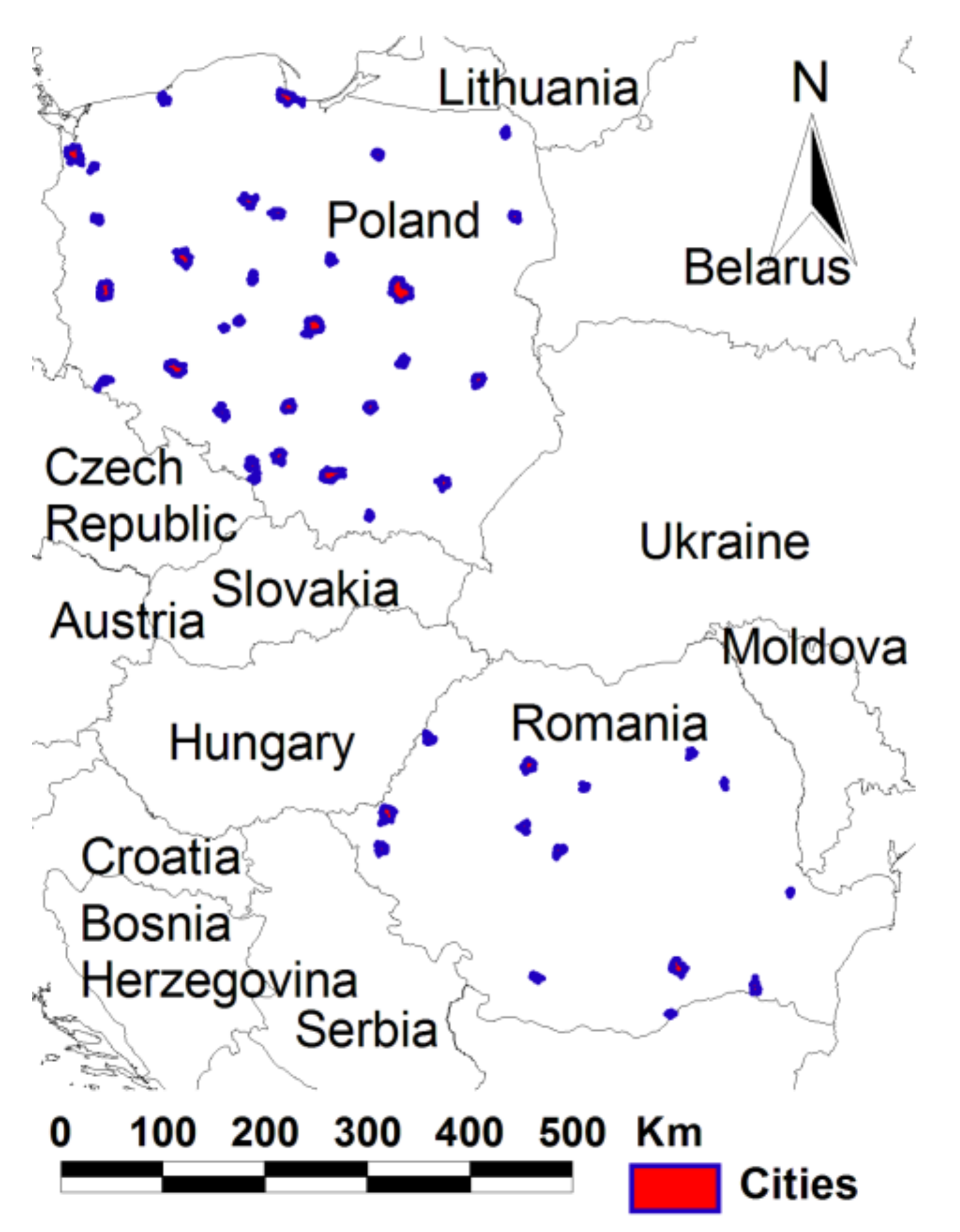

Publisher’s Note: MDPI stays neutral with regard to jurisdictional claims in published maps and institutional affiliations. |
© 2021 by the authors. Licensee MDPI, Basel, Switzerland. This article is an open access article distributed under the terms and conditions of the Creative Commons Attribution (CC BY) license (https://creativecommons.org/licenses/by/4.0/).