Use of Oblique RGB Imagery and Apparent Surface Area of Plants for Early Estimation of Above-Ground Corn Biomass

Abstract

Estimating above-ground biomass in the context of fertilization management requires the monitoring of crops at early stages. Conventional remote sensing techniques make use of vegetation indices such as the normalized difference vegetation index (NDVI), but they do not exploit the high spatial resolution (ground sampling distance < 5 mm) now achievable with the introduction of unmanned aerial vehicles (UAVs) in agriculture. The aim of this study was to compare image mosaics to single images for the estimation of corn biomass and the influence of viewing angles in this estimation. Nadir imagery was captured by a high spatial resolution camera mounted on a UAV to generate orthomosaics of corn plots at different growth stages (from V2 to V7). Nadir and oblique images (30° and 45° with respect to the vertical) were also acquired from a zip line platform and processed as single images. Image segmentation was performed using the difference color index Excess Green-Excess Red, allowing for the discrimination between vegetation and background pixels. The apparent surface area of plants was then extracted and compared to biomass measured in situ. An asymptotic total least squares regression was performed and showed a strong relationship between the apparent surface area of plants and both dry and fresh biomass. Mosaics tended to underestimate the apparent surface area in comparison to single images because of radiometric degradation. It is therefore conceivable to process only single images instead of investing time and effort in acquiring and processing data for orthomosaic generation. When comparing oblique photography, an angle of 30° yielded the best results in estimating corn biomass, with a low residual standard error of orthogonal distance (RSEOD = 0.031 for fresh biomass, RSEOD = 0.034 for dry biomass). Since oblique imagery provides more flexibility in data acquisition with fewer constraints on logistics, this approach might be an efficient way to monitor crop biomass at early stages.

1. Introduction

Since the 1950s, field crops (corn, soybeans, canola, and wheat) have expanded to occupy a greater part of the agricultural landscape in North America. For example, corn (Zea Mays L.) represented 21% of cropland in Quebec in 2016, the most recent numbers according to Statistics Canada [1,2]. This intensified agriculture results in soil degradation and excessive nitrogen use, leading to environmental contamination [3,4] and ultimately, to economic losses [5,6].

To answer those challenges, precision agriculture has emerged as a management strategy that takes into account temporal and spatial variability in order to improve the sustainability of agricultural production [7]. This discipline uses different information and communication technologies in order to collect, process, and analyze multi-source data. In the case of fertilizer management for corn production, the information collected could be used to drive a decision support system in order to act at the right place, at the right time, and with the right quantity [8]. Above-ground biomass, along with chlorophyll content and leaf area index (LAI), is one of the key biophysical parameters for crop monitoring [9]. Therefore, the ability to assess plant-level biomass variations at the field scale is essential for the implementation of novel precision agriculture approaches such as variable nitrogen rate applications [10].

Among the technologies used in precision agriculture, remote sensing platforms are useful for observing, monitoring, and mapping corn growth variability [11]. So-called conventional remote sensing (mostly satellite-borne) operates by modelling the signal from a field crop. Physical or statistical models relate reflectance measures in one or more spectral bands to a given biophysical parameter that expresses the productivity of the crop in some way [11,12]. Estimating vegetation biomass early in the season is critical because many crop management decisions are made when the plant is still at an early growth stage and it is still possible to access the field with machinery without damaging the crop. However, because of their coarse spatial resolutions, satellite-based images present mixels [13], which are defined as pixels containing heterogeneous information from several objects such as the canopy and the underlying soil. Noise attributable to soil effects, the presence of weeds, or cover crops make it difficult to use vegetation indices to adequately estimate crop biomass [14]. Proximal active sensors [15] embedded on heavy agricultural machinery face the same problems [16,17].

The advent of unmanned aerial vehicles (UAVs) has provided an alternative to overcome these problems. Compared to conventional platforms, they offer greater deployment flexibility, shorter revisit times, and better spatial resolution with low atmospheric interference. Compared to proximal sensors, they enable much more flexible logistics and do not impinge on the crop [18,19]. In the context of crop biomass assessment, a UAV equipped with a very high spatial resolution camera is a suitable tool for monitoring biomass at the plant scale, which is still not possible with other remote sensing platforms [20,21]. However, information extraction is still focused on spectral-based approaches relying on vegetation indices [16,22], mostly NDVI (Normalized Difference Vegetation Index) [23]. Although vegetation indices are well-correlated with some biophysical characteristics such as LAI or fresh biomass, their use in the context of high spatial resolution images acquired by UAV-based platforms is not always optimal [24] and requires sophisticated multispectral cameras, presenting challenges in geometric and radiometric corrections [25,26,27].

Other studies have instead relied on object-based approaches exploiting image spatial resolution to extract biophysical parameters through structural features. For example, canopy height can be estimated by photogrammetry and validated with field measurements [28,29,30]. Fractional vegetation cover (FVC) [31,32], plant counting [33,34], or weed detection at early post-emergence [35] are building on the high spatial resolution. Biomass assessment could also benefit from this approach, but this does not seem to be the case yet.

In remote sensing, information is generally extracted from images with the nadir view, i.e., directly above the vertical. This angle of observation is inherent to most optical sensors onboard satellites and is mainly adopted for aerial and UAV platforms. The different biophysical parameters of the plant are thus estimated according to the physical or spectral features of the canopy projected onto the horizontal plane. Furthermore, there is a propensity to generate orthomosaics from UAV imagery for crop monitoring, which imposes image acquisition using the nadir view [36].

Because they can see hidden parts of buildings, oblique (i.e., off-nadir) images have been used to improve 3D reconstruction [37], urban planning, or damage estimation [38]. In agriculture, stereo oblique imagery has been used to generate crop-surface models of barley [39,40]. The ability to measure plant height and LAI from 3D point clouds that were derived from UAV nadir and oblique imagery has also been investigated [36]. Those few studies required the use of photogrammetry and the generation of a spatially continuous model of the canopy. However, single images are rarely used to assess crop parameters, whether in nadir or oblique mode [41]. Our study therefore aims to bridge this gap.

The objective of this research was to assess corn biomass in space and time at early growth stages using images at high spatial resolution. Imagery was acquired with a simple consumer-grade RGB camera mounted on a UAV and on a zip line. We evaluated the impact of using mosaics and single images as well as different viewing angles to estimate corn biomass.

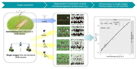
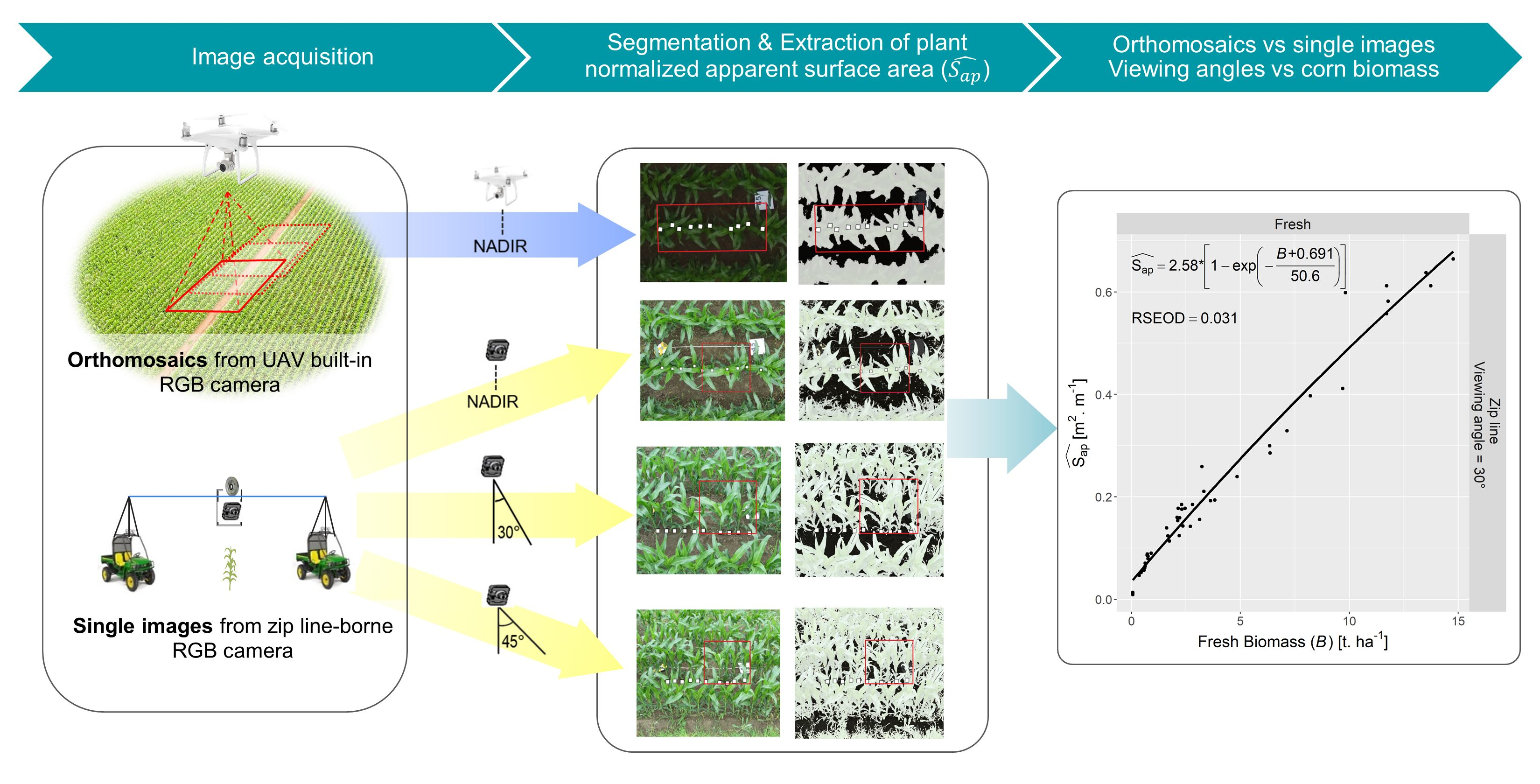
2. Materials and Methods

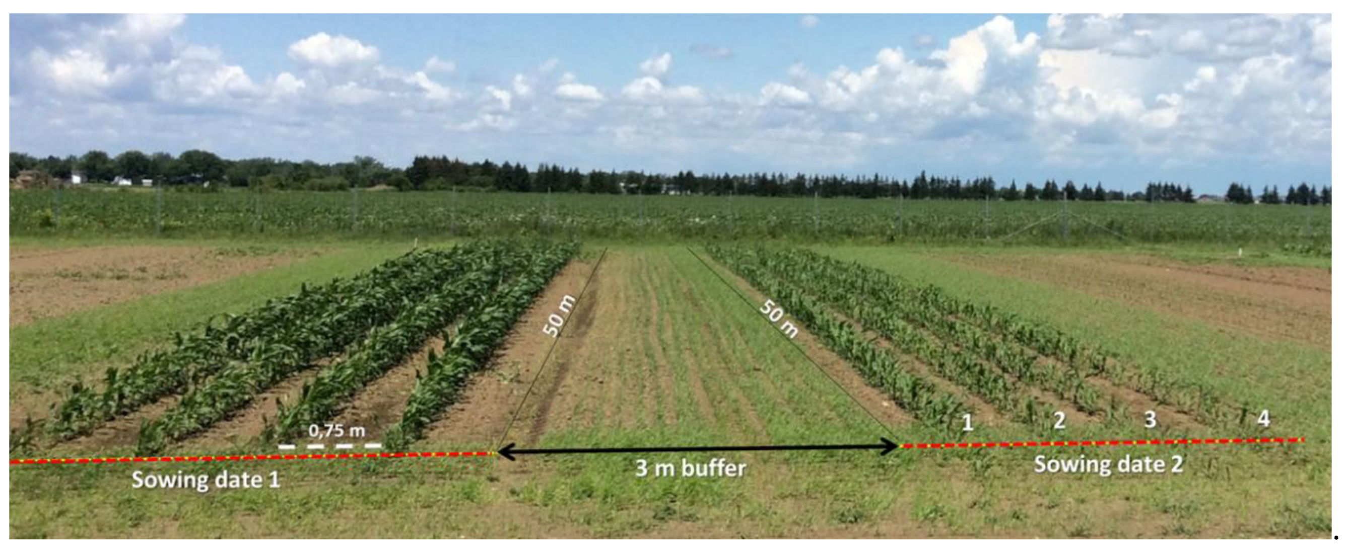
2.1. Study Site

The experiment was conducted at the L’Acadie farm (45°17′40″N, 73°20′45″W), an experimental farm of Agriculture and Agri-Food Canada, located in St-Jean-sur-Richelieu, Quebec. A field of approximately 0.5 ha (100 m × 50 m) was selected for the experiment in the 2017 summer season. Field corn (Zea mays L., cultivar Pioneer P9623, 2850 CHU) was planted (seeding rate fixed at 82,000 seeds ha⁻¹) using an inter-row spacing of 0.75 m. Fertilizer level at seeding was set according to the needs and the soil tests previously carried out. Since we never exceeded the V10 stage, no N fertilizer was applied at mid-season. Weed control was performed mechanically. The field was further divided laterally into four-row plots, with a 3 m buffer zone between each plot (Figure 1). A total of 15 plots were used with different sowing dates such that a diversity of stages (from V2 to V7, 10–40 days after sowing) was present for each data acquisition campaign. Vegetative stages were determined using the V-stages method, based on the number of visible collars [42].

During the experiment, a weekly ground truth campaign was conducted at the same time as the image acquisition. Each ground reference was randomly selected and consisted of two row sections with ten consecutive corn plants each. Only the two middle rows of each plot were used to avoid border effects. The first and the tenth plants of each row-section were identified with a golf tee positioned next to them. After image acquisition, the ten (10) sampled plants of each row were clipped at ground level and weighed individually using a high-precision balance to determine the fresh biomass. The samples were then dried at 70 °C for a minimum of 5 days, and weighed again to get the dry biomass.

Since the purpose of this experiment was to assess the ability of remote sensing to estimate corn biomass, it was important to obtain a diversity of biomass values from our samples. The boxplots in Figure 2 shows the range of biomass values for our ground references and how they increase according to the growth stages.

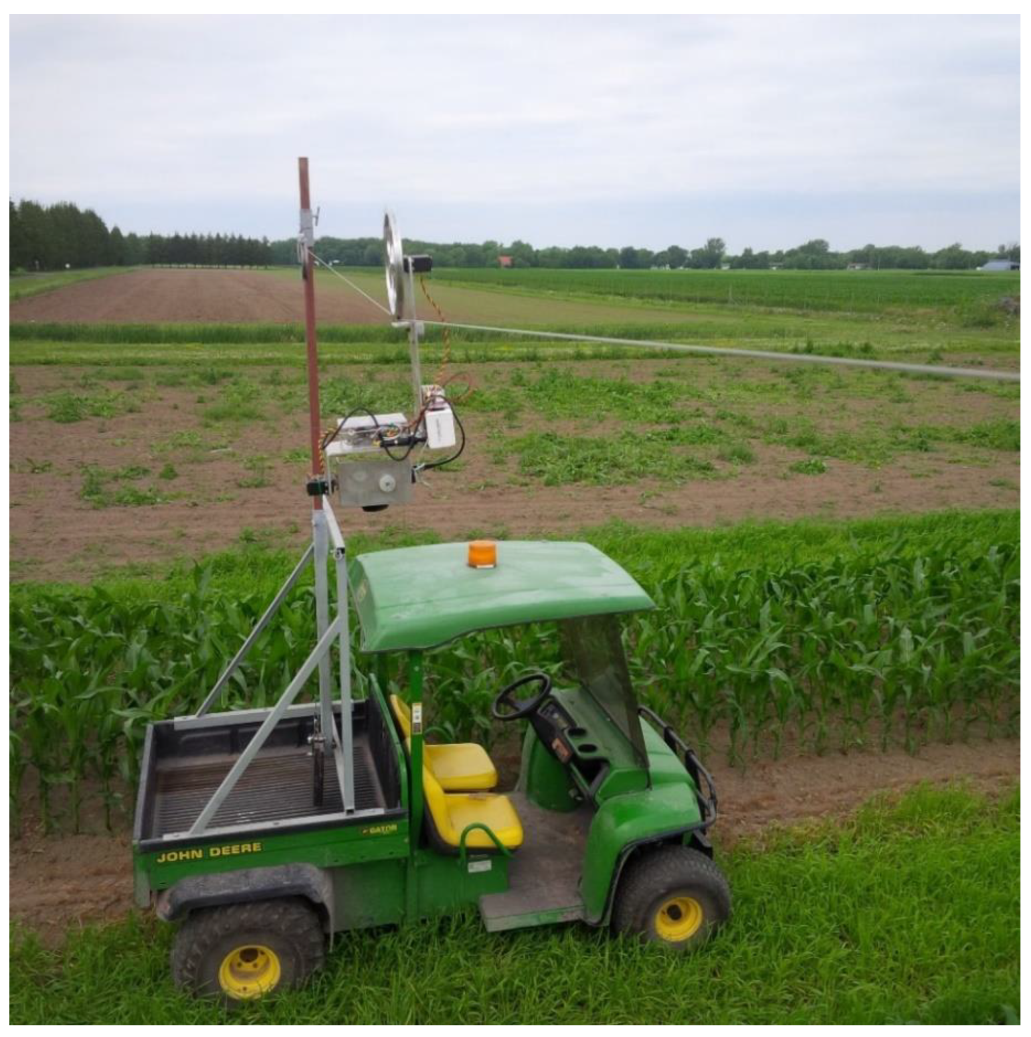
2.2. RGB Imagery Acquisition

Two modes of acquisition were used for this experiment, using two different platforms: a UAV and a zip line, each collecting different types of images and requiring different preprocessing steps.

The first acquisition mode consisted in flying a Phantom 3 Professional UAV (DJI, Shenzen, China) over the field at an altitude of 10 m above ground level (m AGL) following an S-pattern, using the DJI GS GO app (installed on Apple OS, iPad Mini). This mode allowed for the creation of orthomosaics with a ground sampling distance (GSD) of 4.4 mm. The camera used was the UAV built-in camera whose technical characteristics are given in

Table 1. Technical specifications of the cameras used for image acquisition.

Platform	UAV	Zip Line
Camera sensor	1/2.3" CMOS	1/2.3" CMOS
Sensor width (mm)	6.30	6.16
Sensor height (mm)	4.73	4.62
Image size (pixels)	4000 × 3000	4000 × 3000
Focal length (mm)	3.6	5.0
Diagonal field of view	95°	75°
Pixel dimension (μm)	1.58	1.54
Acquisition mode	Flight path (S-pattern)	Stationary
Acquisition altitude (m AGL)	10	2.9
Viewing angles	Nadir (0°)	Nadir (0°) and oblique (30° and 45°)
Generated products	Orthomosaics	Single images
GSD (mm)	4.4	0.89 (viewing angle = 0°) 1.03 (viewing angle = 30°) 1.26 (viewing angle = 45°)

. The autonomy of this UAV was sufficient to produce an image our small experimental field in one flight. To increase the success of image stitching, flight paths were planned with a minimum overlap of 70% (lateral and longitudinal overlaps). The acquired images were imported into the Pix4Dmapper Pro software (Pix4D SA, Lausanne, Switzerland) and an orthomosaic was generated using ground control points (GCPs) located in the corner of each plot (4 per plot) and in the center of the field. Each GCP was positioned with a Real-Time Kinematics (RTK) Global Navigation Satellite System (GNSS) receiver (SXBlue III-L, Geneq Inc., Montreal, QC, Canada). Eight flyovers (5, 12, 18, 26, 31 July; 7, 18, 25 August) were carried out, but only seven were successful in generating an orthomosaic. For the first flight (5 July), the target coverage rate of 70% was not achieved due to missing images (the camera’s memory card was not capable of recording images fast enough and was upgraded for the remaining flights).

The second acquisition mode consisted in capturing pictures at selected ground references with different viewing angles. From preliminary works [43], we realized that our UAV platform was not stable enough to acquire images in such a stationary mode, i.e., hovering above the same point. A custom zip line was thus designed and constructed to provide a stable and easy-to-use platform for acquiring RGB images in stationary mode (Figure 3). A steel cable was stretched between two posts attached to utility task vehicles (UTV, Gator, John Deere, Moline, IL). A Canon SX230 HS (Canon Inc., Tokyo, Japan) camera was suspended from the cable at 2.9 m AGL (see camera characteristics in Table 1). To produce a ground reference image, both UTVs were positioned on each side of a plot so that the cable ran perpendicularly to the rows. The camera was remotely controlled and the viewing angle was set to 0° (nadir), 30°, or 45° with respect to the vertical for the oblique images. Geometric image distortions due to the camera lens were roughly corrected by the camera internal software and no further image corrections were applied. This mode generated single images, with GSD between 0.89 mm and 1.26 mm, varying according to the viewing angle. The GSD was calculated for the pixel in the center of the image located on the plane orthogonal to the camera’s optical axis and containing the stem of the corn plants. The distance between the camera and the target had to be adjusted according to the viewing angle since the height of the platform was constant.

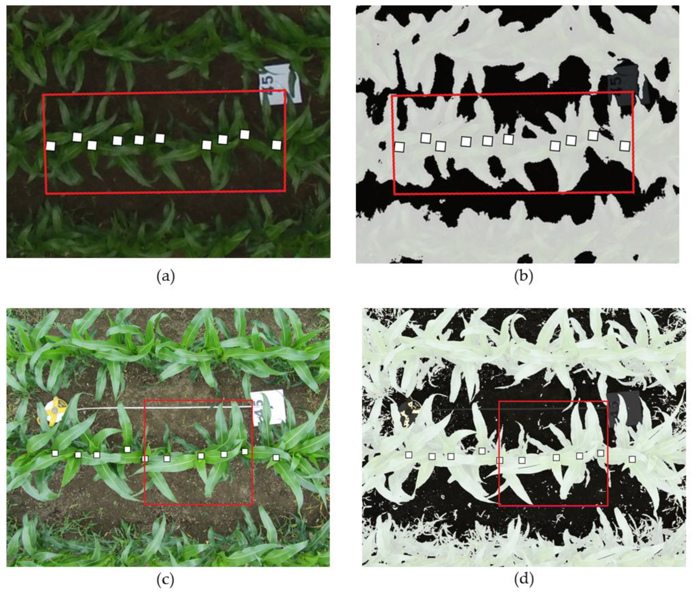
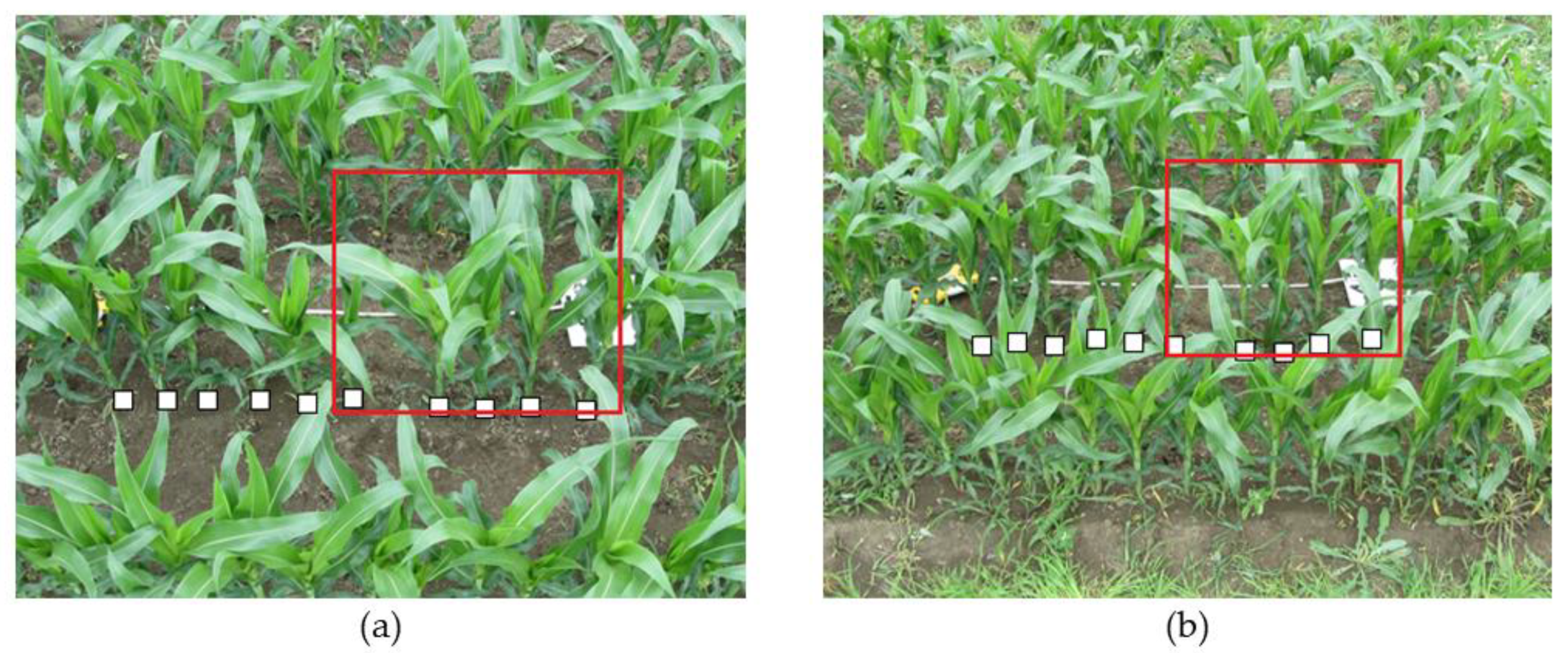
2.3. Information Retrieval from RGB Imagery

In order to compare the two acquisition modes and their results with the ground truth, the ground references had to be located and delineated in the images (orthomosaics and single images). This task was performed manually through a custom graphical user interface (GUI) developed in Python using the graphical toolkit Tkinter [44]. The images were then segmented to distinguish vegetation from the background. Finally, apparent surface area was calculated and correlated with biomass measurements.

For the UAV mode, the orthomosaics generated from the images were first cut into thumbnails of approximately 800 × 800 pixels (about 3.5 m × 3.5 m), each centered on a ground reference. Within each thumbnail, the 2 sampled row sections were located. Then, each row was manually delineated by drawing a rectangle around the 10 sampled plants to define a quadrat (Figure 4a). For the zip line mode, each single image was processed sequentially. The 10 plants whose weight was measured were identified through visual inspection. A virtual quadrat measuring 1 m in length was subsequently positioned on the sampled row and only the plants contained in this rectangle were used as ground truth reference, with their biomass computed and apparent surface extracted. The number of plants in each quadrat varied between 5 and 8, depending on the density of the row. Because of the short distance between the camera and the target, the 10 sampled plants were not always visible in the same image, and pixels near the image borders were distorted because of the central perspective. Hence, the quadrat was set to be 1-m long and was positioned close to the center of the image. The width of the quadrat was manually chosen to enclose most vegetation surfaces belonging to the sampled plants while minimizing the surfaces from the adjacent rows. In the nadir images, the width corresponded roughly to the inter-row spacing, i.e., 0.75 m (Figure 4c). For the oblique images, the quadrat was wider to encompass the full height of the corn plants (Figure 5a,b), and no attempt was made to exclude overlapping leaves from adjacent rows. That processing would have needed to be performed manually or would have required a more complex image segmentation algorithm.

The image segmentation was entirely executed with a custom Python script using the OpenCV v3.4.0.12 [45] and NumPy v1.14.0 [46] modules. Each RGB image (orthomosaic thumbnail or single image) was converted to an ExG-ExR image using Equation (2) [47]. This proved to be particularly effective and more accurate than the other color indices that were tested. To compute the indices, the RGB images needed to be converted to RGB chromaticities:

$$\begin{gathered} r=\frac{\mathrm{R}}{\mathrm{R}+\mathrm{G}+\mathrm{B}} \\ g=\frac{\mathrm{G}}{\mathrm{R}+\mathrm{G}+\mathrm{B}} \\ b=\frac{\mathrm{B}}{\mathrm{R}+\mathrm{G}+\mathrm{B}} \end{gathered}$$

(1)

Then, ExG-ExR was computed:

$$ExG-ExR=\left(2g-r-b\right)-\left(1.4r-g\right)=3g-2.4r-b$$

(2)

Thresholding the ExG-ExR image is simple since the index is positive for vegetation pixels and negative for background pixels [47].

2.4. Statistical Analysis

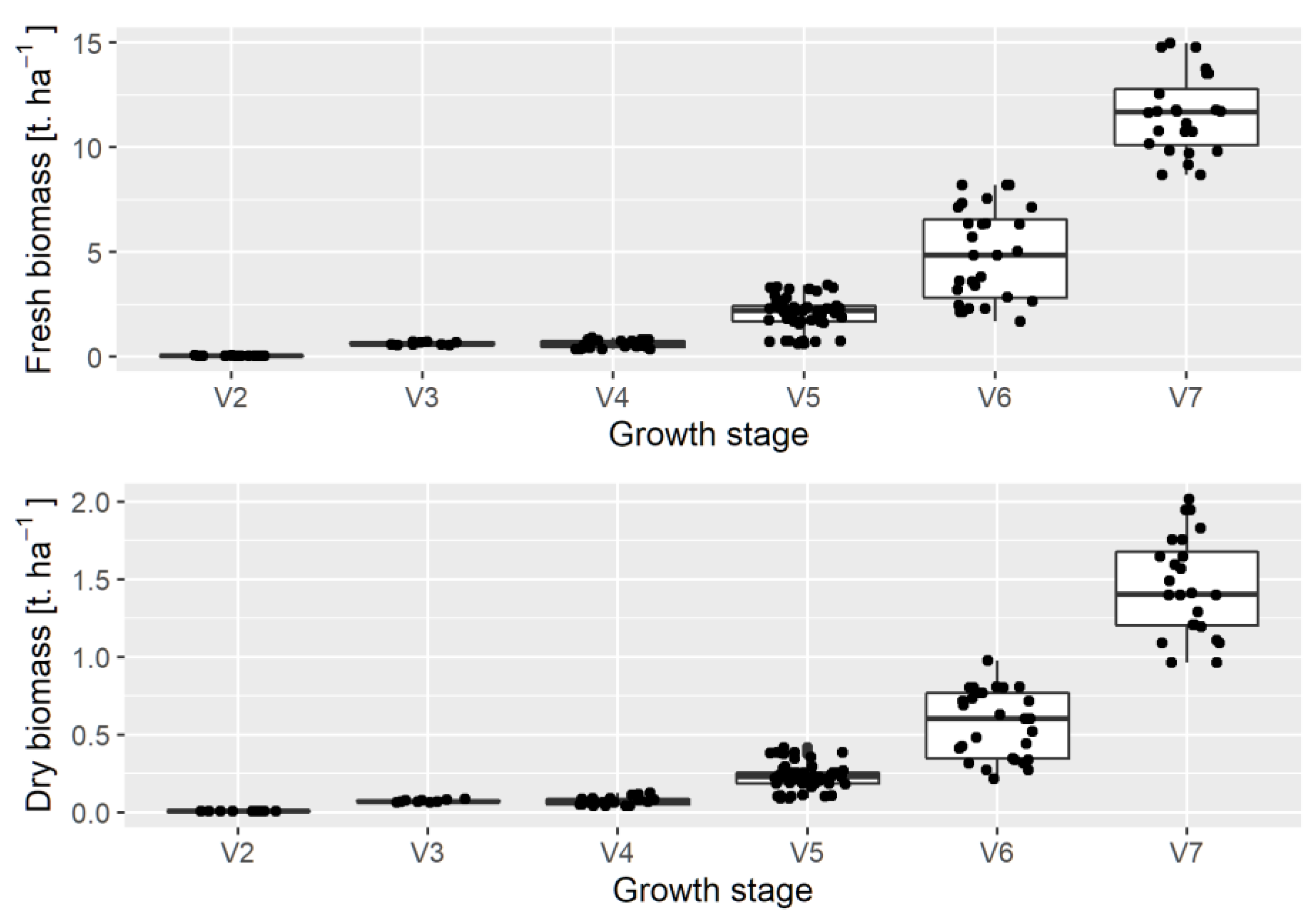
The information extracted from the images was the apparent surface area of the plants. In order to confirm that the apparent surface could be a good proxy for biomass, a regression analysis was performed to define the relationship between the two.

For each RGB image, the segmentation step generated a binary image (Figure 4b,d), where pixels corresponding to vegetation had a value of 1 and background pixels were 0. Summing up the value of all pixels in a quadrat Q, the number $N_v$ of vegetation pixels in that quadrat was thus:

$$N_{\mathrm{v}}\left(\mathsf{\alpha }\right)={\displaystyle \sum }_{\mathrm{i}\in \mathrm{Q}}{p}_{\mathrm{i}}$$

(3)

where

$N_v$: number of vegetation pixels in quadrat Q;

α: the viewing angle;

$p_i$: 1 if pixel i belongs to the vegetation class, 0 otherwise. The apparent surface area of the plant ${\mathrm{S}}_{\mathrm{ap}}$ in square meters was calculated as follows:

$${\mathrm{S}}_{\mathrm{ap}}\left(\mathsf{\alpha }\right)=N_v\left(\mathsf{\alpha }\right)·\rho {\left(\mathsf{\alpha }\right)}^2$$

(4)

where $\rho \left(\mathsf{\alpha }\right)$ is the GSD in meters, a function of the viewing angle α. To simplify notation, the angular dependence will be omitted in the following text.

The pixel count included both leaves and plant stems, especially when viewed at an oblique angle (α > 0°). In addition, the calculated area was called apparent because only the vegetation pixels visible in the image were considered. The size of the objects represented by those pixels was considered constant and equal to the GSD, regardless of their actual distance from the camera, with the 3D position of each pixel being unknown.

Finally, the ${\mathrm{S}}_{\mathrm{ap}}$ values were divided by the length of the quadrat to obtain normalized apparent surface area values ($\widehat{{\mathrm{S}}_{\mathrm{ap}}}$), independent of the length of the rectangle drawn. $\widehat{{\mathrm{S}}_{\mathrm{ap}}}$ was calculated as follows:

$$\widehat{{\mathrm{S}}_{\mathrm{ap}}}=\frac{{\mathrm{S}}_{\mathrm{ap}}}{L}=\frac{{\mathrm{N}}_v{\mathsf{\rho }}^2}{L}$$

(5)

where $L$ is the length of the quadrat in meters (1.2 m $\le L\le$ 1.9 m for the UAV mode, $L=1$m for the zip line mode). It is thus the surface area measured per unit length along a row in m²·m⁻¹.

Above-ground biomass $B$ (in kg·m⁻²) inside each quadrat was calculated for each row section using:

$$B=\frac{{\sum }_{\mathrm{i}=1}^{\mathrm{N}}{M}_{\mathrm{i}}}{L}$$

(6)

where $L$ is the length of the quadrat in meters, $M_{\mathrm{i}}$ is the fresh or dry weight of plant i in kilograms, and $\mathrm{N}$ the number of plants inside the quadrat ($\mathrm{N}=10$ for the UAV mode, $5\le \mathrm{N}\le 8$ for the zip line mode). Biomass was then rescaled to tons per hectare (t·ha⁻¹).

A regression model was constructed from the training dataset to explain the behavior of the dependent variable $\widehat{{\mathrm{S}}_{\mathrm{ap}}}$ as a function of the independent variable $B$ representing the corn biomass. Because of measurement errors in both independent and dependent variables, the orthogonal (or total) least squares regression was preferred to the ordinary least squares regression [48]. Details about the algorithm can be found in the vignette of the onls R package [49] that was used in this paper. The goodness of fit of the model was based on the Residual Standard Error of Orthogonal Distance (RSEOD) [48].

3. Results

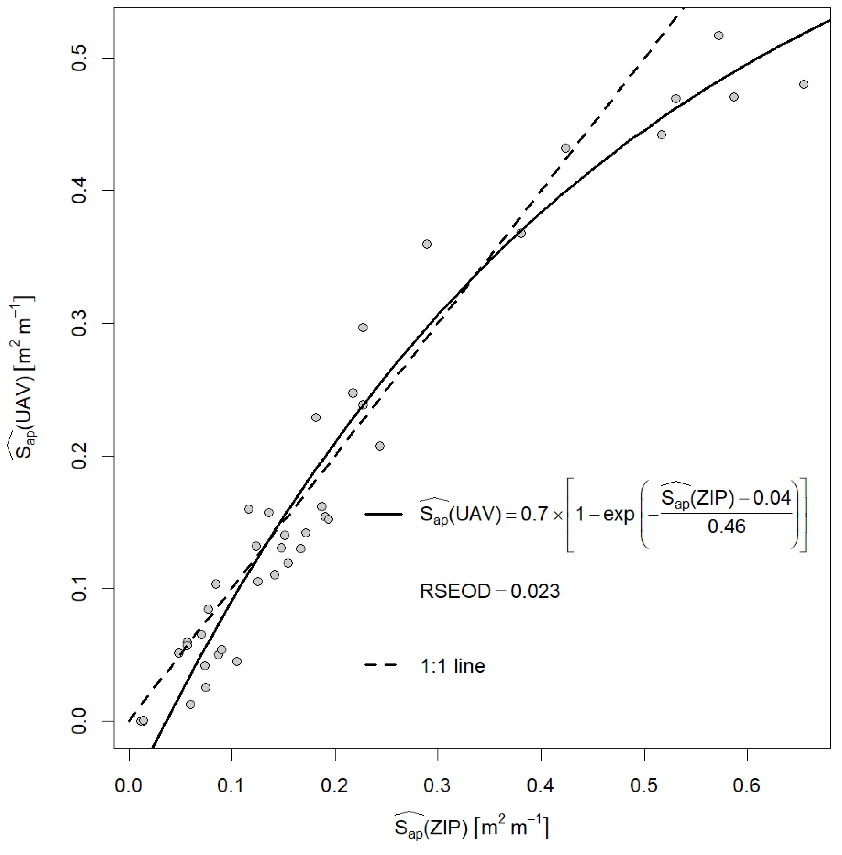
3.1. Comparing UAV and Zip Line at Nadir View

At nadir view, both modes gave slightly different values for the normalized apparent surface area $\widehat{{\mathrm{S}}_{\mathrm{ap}}}$. The UAV mode tended to underestimate $\widehat{{\mathrm{S}}_{\mathrm{ap}}}$ for low and high biomass values. Figure 6 shows that there is an asymptotic relationship (non-linear total least-squares) between $\widehat{{\mathrm{S}}_{\mathrm{ap}}}\left(\mathrm{UAV}\right)$ calculated from the UAV platform, and $\widehat{{\mathrm{S}}_{\mathrm{ap}}}\left(\mathrm{ZIP}\right)$ calculated from the zip line platform, with an RSEOD of 0.023. The regression curve was not forced to pass through the origin due to the incertitude in image processing, as the algorithm might detect crops when there is no vegetation or vice versa. A linear total least squares fit yielded a RSEOD of 0.029 (data not shown).

The regression models at nadir view show a good asymptotic relationship between $\widehat{{\mathrm{S}}_{\mathrm{ap}}}$ and both dry (Figure 7a,c) and fresh (Figure 7b,d) biomass. Asymptotic coefficients for the UAV mode (Figure 7a,b) have lower values than those for the zip line mode (Figure 7c,d), suggesting a quicker saturation of $\widehat{{\mathrm{S}}_{\mathrm{ap}}}$ for the UAV at high biomass values. Still, RSEODs are very similar between both modes, despite orthomosaics being fraught with geometric and radiometric degradations.

3.2. The Effect of Viewing Angles

Figure 7c–h show the effects of the viewing angle in estimating the normalized apparent surface area $\widehat{{\mathrm{S}}_{\mathrm{ap}}}$ extracted from the zip line mode using the measured biomass as ground truth. There is an asymptotic relationship between $\widehat{{\mathrm{S}}_{\mathrm{ap}}}$ and corn biomass, with RSEODs ranging from 0.031 to 0.040 for fresh biomass, and from 0.034 to 0.045 for dry biomass. Clearly, dry biomass is strongly correlated with fresh biomass, and $\widehat{{\mathrm{S}}_{\mathrm{ap}}}$ is a good indicator of both fresh and dry biomass for all three viewing angles.

Since horizontal surfaces appear smaller as viewing angles increase, areas from more vertical surfaces and other hidden surfaces compensate in oblique imagery. The apparent increase in the asymptotic coefficients with increasing viewing angles may be an indication that this compensation is more efficient at larger viewing angles. However, when considering the RSEODs, it seems that a viewing angle of 30° results in the best fit (RSEOD ≈ 0.03) among the three angles that were tested (RSEOD ≈ 0.04 for viewing angles of 0° and 45°).

4. Discussion

In this study, a novel parameter—the normalized apparent surface area $\widehat{{\mathrm{S}}_{\mathrm{ap}}}$—has been proposed to monitor corn biomass at the row level. The $\widehat{{\mathrm{S}}_{\mathrm{ap}}}$ appears to be a good proxy of both fresh and dry corn biomass, with a good regression fit.

Even so, the application of this method requires vegetation to be clearly discriminated from the background. In this study, image segmentation produced consistent results because the spatial resolution was high enough. Rasmussen et al. [50] found that the discrimination of crops from the background in the early stages of barley growth required ultra-fine resolution images (GSD < 5 mm). In our experiment, the highest GSD (i.e., the lowest spatial resolution) was 4.4 mm for the UAV mode and 1.26 mm for the zip line mode. The ExG-ExR color index used for image segmentation resulted in a binarized image that distinguished plants from the background. Thus, green pixels also included weeds if they were present. However, the use of oblique images minimizes the importance of weeds since they were shorter than the measured corn plants. If a plot is invaded by weeds, the $\widehat{{\mathrm{S}}_{\mathrm{ap}}}$ estimate would be distorted if they were not excluded from the calculation. Detecting weeds should then be a preliminary step, using techniques such as feature [51] or texture recognition [52], hyperspectral imagery [53,54], or deep learning [55,56].

The lower spatial resolution for orthomosaics is expected to generate less accurate segmentation (Figure 4b). Although there is an underestimation of the $\widehat{{\mathrm{S}}_{\mathrm{ap}}}$ from the orthomosaics at low and high values (Figure 6), the regression curve is still close to the 1:1 line. The underestimation of corn biomass with the UAV mode is likely attributable to the degradation of geometric and radiometric quality resulting from mosaicking (gaps in the mosaic, incorrect stitching, artifacts, blurs, etc.). The final vegetation mosaic is not necessarily satisfactory and is highly dependent on acquisition conditions (camera exposure, coverage rate, canopy architecture). Poor photogrammetric results at this level of details produce approximate segmentation, as evidenced in Figure 4b. It would therefore be advantageous in terms of processing time and effort to only use single images for crop biomass estimation. With a precise location measured with RTK GNSS, each single image can be processed to calculate the biomass of the plant at a specific point in the field.

With the stationary mode, a range of off-nadir viewing angles can also be chosen with little effect on the estimation of the biomass (Figure 7). However, an angle of 30° could be the most logical choice to estimate corn biomass as, while focusing less on horizontal leaves, it reveals more of the vertical structure of the plants. At an angle of 45°, the regression yields a higher RSEOD, which suggests that the compensation effect of vertical surfaces may subside with steeper viewing angles (angles > 45° were not tested because of their impracticality in the context of a corn field). The effect of leaf angle, i.e., the proportion of flat to upright surfaces inherent to each cultivar and each growth stage, should be considered as that factor will influence the results.

For the nadir view, the normalized apparent surface area $\widehat{{\mathrm{S}}_{\mathrm{ap}}}$ can be retrieved from the fractional vegetation cover (FVC), which is expressed as the ratio of the vegetation area ${\mathrm{S}}_{\mathrm{ap}}$to the sampling area ${\mathrm{S}}_{\mathrm{z}}$, as projected on the horizontal plane:

$$FVC=\frac{{\mathrm{S}}_{\mathrm{ap}}}{{\mathrm{S}}_{\mathrm{z}}}=\frac{{\mathrm{S}}_{\mathrm{ap}}}{Lw}=\frac{\widehat{{\mathrm{S}}_{\mathrm{ap}}}}{w}$$

(7)

where $L$ and $w$ are respectively the length and width of the sampling area. When dealing with one row, w is equivalent to the inter-row spacing. FVC is only valid for images acquired at nadir. In an oblique image, the vegetation surface taken into consideration is no longer limited by the sampling area. Normalizing ${\mathrm{S}}_{\mathrm{ap}}$ by a cosine factor would imply that all or most imaged surfaces are horizontal, which is clearly not the case for corn plants. There is another way to normalize vegetation area for row crops such as corn that was adopted here: the vegetation area per row length $\widehat{{\mathrm{S}}_{\mathrm{ap}}}$ as in Equation (5). With that parameter, oblique imagery can only focus on a single row at a time because other rows are partially hidden and pixels distant from the perspective center are too distorted.

Proximal active sensors and satellite images have a limitation for monitoring crops at early growth stages [17,57] since the signal from the vegetation cover is not strong enough to overcome the noise from bare soil. Moreover, they tend to rely on spectral-based approaches that depend on geometric and radiometric acquisition conditions [41,58,59,60,61]. The method described here is interesting because it requires only the discrimination of vegetation from soil, which is easily applicable at the growth stages considered. It makes early crop monitoring possible at a time when crop management decisions matter the most. Indeed, farmers applying spatially variable interventions to their crops need to react as early as possible to maximize the benefits at harvest, which is currently hardly possible due to the lack of sensitivity with the use of other remote sensing approaches. A simple set-up using an RGB camera mounted on a tractor boom to capture oblique images could be used for the crop biomass estimation of incoming plants prior to in-season fertilization. This could be performed during mechanical or chemical weed control occurring prior to in-season fertilization.

5. Conclusions

This study explored an alternative to vegetation indices for predicting corn biomass from images with very high spatial resolution. By segmenting the images and calculating the $\widehat{{\mathrm{S}}_{\mathrm{ap}}}$, it was possible to estimate corn biomass with good accuracy. Although segmentation was less accurate with orthomosaics than single images, both platforms (UAV and zip line) yielded good estimations of corn biomass at nadir view. Our study demonstrated that using oblique imagery at 30° could improve biomass estimation, although differences between the nadir and oblique viewing angles up to 45° are not that significant. Further investigation should aim at a wider range of viewing angles.

The $\widehat{{\mathrm{S}}_{\mathrm{ap}}}$ can be quickly extracted from a single image or a mosaic. However, mosaicking not only imposes a significant effort on the acquisition and processing of images, but also generates artifacts because of the degradation of radiometric quality and the instabilities of the UAV platform. The apparent surface calculated from an RGB camera is easy to obtain (simple processing, no reflectance to calculate) and gives a good estimate of corn biomass in space and time. Moreover, this method would allow for biomass estimation at row scale. It is therefore feasible to perform crop management either by zone or by row. Likewise, we believe that this method would benefit from being tested on other crops (wheat, soybeans, or vegetables).

It is currently difficult to have a good estimation of biomass at the beginning of the season. With this novel way of assessing crop biomass, it is possible to use robotic platforms in agriculture such as autonomous robots [62] and drones. High spatial resolution images are also possible with cell phones and other IoT (Internet of Things)-connected devices [63]. A better understanding of their pros and cons would necessitate further research. We suggest that this novel $\widehat{{\mathrm{S}}_{\mathrm{ap}}}$ measure, at a relevant angle of acquisition, can be used for early crop biomass estimations in combination with more traditional measurements such as the NDVI value. Since oblique imagery can provide a good estimation of crop biomass, those platforms do not need to be directly above a target point. In addition, oblique camera viewing allows for wider coverage, reducing the number of images to be processed. Future work will investigate the application of the $\widehat{{\mathrm{S}}_{\mathrm{ap}}}$ measure on single plants and other crops. We will also evaluate potential applications in identifying crop deficiency at early growth stages.

References

1. Statistics Canada. Table32-10-0406-01 Land Use. Available online: https://www150.statcan.gc.ca/t1/tbl1/en/tv.action?pid=3210040601 (accessed on 29 April 2021).
2. Statistics Canada. Table32-10-0416-01 Hay and field crops. Available online: https://www150.statcan.gc.ca/t1/tbl1/en/tv.action?pid=3210041601 (accessed on 29 April 2021).
3. Tilman, D.; Cassman, K.G.; Matson, P.A.; Naylor, R.; Polasky, S. Agricultural sustainability and intensive production practices. Nature 2002, 418, 671–677. [Google Scholar] [CrossRef] [PubMed]
4. Tremblay, N.; Bélec, C. Adapting Nitrogen Fertilization to Unpredictable Seasonal Conditions with the Least Impact on the Environment. Horttechnology 2006, 16, 408–412. [Google Scholar] [CrossRef] [Green Version]
5. Schröder, J.J.; Neeteson, J.J.; Oenema, O.; Struik, P.C. Does the crop or the soil indicate how to save nitrogen in maize production?: Reviewing the state of the art. Field Crop. Res. 2000, 66, 151–164. [Google Scholar] [CrossRef]
6. Shanahan, J.F.; Kitchen, N.R.; Raun, W.R.; Schepers, J.S. Responsive in-season nitrogen management for cereals. Comput. Electron. Agric. 2008, 61, 51–62. [Google Scholar] [CrossRef] [Green Version]
7. Precision Ag Definition. Available online: https://www.ispag.org/about/definition (accessed on 27 April 2021).
8. Longchamps, L.; Khosla, R. Precision maize cultivation techniques. In Burleigh Dodds Series in Agricultural Science; Cgiar Maize Research Program Manager, C.M., Watson, D., Eds.; Burleigh Dodds Science Publishing Limited: Cambridge, UK, 2017; pp. 107–148. [Google Scholar]
9. Yu, Z.; Cao, Z.; Wu, X.; Bai, X.; Qin, Y.; Zhuo, W.; Xiao, Y.; Zhang, X.; Xue, H. Automatic image-based detection technology for two critical growth stages of maize: Emergence and three-leaf stage. Agric. Forest Meteorology. 2013, 174–175, 65–84. [Google Scholar] [CrossRef]
10. Corti, M.; Cavalli, D.; Cabassi, G.; Vigoni, A.; Degano, L.; Marino Gallina, P. Application of a low-cost camera on a UAV to estimate maize nitrogen-related variables. Precis. Agric. 2018. [Google Scholar] [CrossRef]
11. Mulla, D.J. Twenty five years of remote sensing in precision agriculture: Key advances and remaining knowledge gaps. Biosyst. Eng. 2013, 114, 358–371. [Google Scholar] [CrossRef]
12. Xue, J.; Su, B. Significant remote sensing vegetation indices: A review of developments and applications. J. Sensors 2017, 2017. [Google Scholar] [CrossRef] [Green Version]
13. Quintano, C.; Fernández-Manso, A.; Shimabukuro, Y.E.; Pereira, G. Spectral unmixing. Int. J. Remote Sens. 2012, 33, 5307–5340. [Google Scholar] [CrossRef]
14. Basso, B.; Cammarano, D. Remotely sensed vegetation indices: Theory and applications for crop management. Ital. J. Agrometeorol. 2004, 1, 36–53. [Google Scholar]
15. Holland, K.H.; Lamb, D.W.; Schepers, J.S. Radiometry of Proximal Active Optical Sensors (AOS) for Agricultural Sensing. IEEE J. Sel. Top. Appl. Earth Obs. Remote Sens. 2012, 5, 1793–1802. [Google Scholar] [CrossRef]
16. Corti, M.; Cavalli, D.; Cabassi, G.; Marino Gallina, P.; Bechini, L. Does remote and proximal optical sensing successfully estimate maize variables? A review. Eur. J. Agron. 2018, 99, 37–50. [Google Scholar] [CrossRef]
17. Tremblay, N.; Wang, Z.; Ma, B.-L.; Belec, C.; Vigneault, P. A comparison of crop data measured by two commercial sensors for variable-rate nitrogen application. Precis. Agric. 2009, 10, 145–161. [Google Scholar] [CrossRef]
18. Zhang, C.; Kovacs, J.M. The application of small unmanned aerial systems for precision agriculture: A review. Precis. Agric. 2012, 13, 693–712. [Google Scholar] [CrossRef]
19. Hunt, E.R.; Daughtry, C.S.T.; Mirsky, S.B.; Hively, W.D. Remote sensing with unmanned aircraft systems for precision agriculture applications. In Proceedings of the 2nd International Conference on Agro-Geoinformatics: Information for Sustainable Agriculture, Fairfax, VA, USA, 12–16 August 2013; pp. 131–134. [Google Scholar] [CrossRef]
20. Ren, X.; Sun, M.; Zhang, X.; Liu, L. A simplified method for UAV multispectral images mosaicking. Remote. Sens. 2017, 9, 962. [Google Scholar] [CrossRef] [Green Version]
21. Maes, W.H.; Steppe, K. Perspectives for Remote Sensing with Unmanned Aerial Vehicles in Precision Agriculture. Trends Plant Sci. 2019, 24, 152–164. [Google Scholar] [CrossRef] [PubMed]
22. Bouroubi, Y.; Tremblay, N.; Vigneault, P.; Bélec, C.; Adamchuk, V. Estimating nitrogen sufficiency index using a natural local reference approach. In Proceedings of the 2nd International Conference on Agro-Geoinformatics: Information for Sustainable Agriculture, Fairfax, VA, USA, 12–16 August 2013; pp. 71–75. [Google Scholar] [CrossRef]
23. Rouse, J.W.; Haas, R.H.; Schell, J.A.; Deering, D.W. Monitoring Vegetation Systems in the Great Plains with ERTS; NASA: Washington, D.C., USA, 1974; pp. 309–317.
24. Hunt, E.R.; Daughtry, C.S.T. What good are unmanned aircraft systems for agricultural remote sensing and precision agriculture? Int. J. Remote Sens. 2018, 39, 5345–5376. [Google Scholar] [CrossRef] [Green Version]
25. Lelong, C.C.D.; Burger, P.; Jubelin, G.; Roux, B.; Labbé, S.; Baret, F. Assessment of unmanned aerial vehicles imagery for quantitative monitoring of wheat crop in small plots. Sensors 2008, 8, 3557–3585. [Google Scholar] [CrossRef] [PubMed]
26. Berni, J.A.J.; Zarco-Tejada, P.J.; Suárez, L.; Fereres, E. Thermal and narrowband multispectral remote sensing for vegetation monitoring from an unmanned aerial vehicle. IEEE Trans. Geosci. Remote Sens. 2009, 47, 722–738. [Google Scholar] [CrossRef] [Green Version]
27. Rabatel, G.; Labbé, S. Registration of visible and near infrared unmanned aerial vehicle images based on Fourier-Mellin transform. Precis. Agric. 2016, 17, 564–587. [Google Scholar] [CrossRef] [Green Version]
28. Holman, F.H.; Riche, A.B.; Michalski, A.; Castle, M.; Wooster, M.J.; Hawkesford, M.J. High throughput field phenotyping of wheat plant height and growth rate in field plot trials using UAV based remote sensing. Remote Sens. 2016, 8, 1031. [Google Scholar] [CrossRef]
29. Hu, P.; Chapman, S.C.; Wang, X.; Potgieter, A.; Duan, T.; Jordan, D.; Guo, Y.; Zheng, B. Estimation of plant height using a high throughput phenotyping platform based on unmanned aerial vehicle and self-calibration: Example for sorghum breeding. Eur. J. Agron. 2018, 95, 24–32. [Google Scholar] [CrossRef]
30. Madec, S.; Baret, F.; de Solan, B.; Thomas, S.; Dutartre, D.; Jezequel, S.; Hemmerlé, M.; Colombeau, G.; Comar, A. High-Throughput Phenotyping of Plant Height: Comparing Unmanned Aerial Vehicles and Ground LiDAR Estimates. Front. Plant Sci. 2017, 8, 2002. [Google Scholar] [CrossRef] [PubMed] [Green Version]
31. Breckenridge, R.P.; Dakins, M.; Bunting, S.; Harbour, J.L.; Lee, R.D. Using Unmanned Helicopters to Assess Vegetation Cover in Sagebrush Steppe Ecosystems. Rangel. Ecol. Manag. 2012, 65, 362–370. [Google Scholar] [CrossRef]
32. Torres-Sánchez, J.; Peña, J.M.; de Castro, A.I.; López-Granados, F. Multi-temporal mapping of the vegetation fraction in early-season wheat fields using images from UAV. Comput. Electron. Agric. 2014, 103, 104–113. [Google Scholar] [CrossRef]
33. Gnädinger, F.; Schmidhalter, U. Digital Counts of Maize Plants by Unmanned Aerial Vehicles (UAVs). Remote Sens. 2017, 9, 544. [Google Scholar] [CrossRef] [Green Version]
34. Varela, S.; Dhodda, P.R.; Hsu, W.H.; Prasad, P.V.V.; Assefa, Y.; Peralta, N.R.; Griffin, T.; Sharda, A.; Ferguson, A.; Ciampitti, I.A. Early-Season Stand Count Determination in Corn via Integration of Imagery from Unmanned Aerial Systems (UAS) and Supervised Learning Techniques. Remote Sens. 2018, 10, 343. [Google Scholar] [CrossRef] [Green Version]
35. Peña, J.M.; Torres-Sánchez, J.; de Castro, A.I.; Kelly, M.; López-Granados, F. Weed Mapping in Early-Season Maize Fields Using Object-Based Analysis of Unmanned Aerial Vehicle (UAV) Images. PLoS ONE 2013, 8. [Google Scholar] [CrossRef] [Green Version]
36. Che, Y.; Wang, Q.; Xie, Z.; Zhou, L.; Li, S.; Hui, F.; Wang, X.; Li, B.; Ma, Y. Estimation of maize plant height and leaf area index dynamics using an unmanned aerial vehicle with oblique and nadir photography. Ann. Bot. 2020, 126, 765–773. [Google Scholar] [CrossRef]
37. Nesbit, P.R.; Hugenholtz, C.H. Enhancing UAV–SfM 3D Model Accuracy in High-Relief Landscapes by Incorporating Oblique Images. Remote Sens. 2019, 11, 239. [Google Scholar] [CrossRef] [Green Version]
38. Kakooei, M.; Baleghi, Y. A two-level fusion for building irregularity detection in post-disaster VHR oblique images. Earth Sci. Inform. 2020, 13, 459–477. [Google Scholar] [CrossRef]
39. Brocks, S.; Bendig, J.; Bareth, G. Toward an automated low-cost three-dimensional crop surface monitoring system using oblique stereo imagery from consumer-grade smart cameras. J. Appl. Remote Sens. 2016, 10, 046021. [Google Scholar] [CrossRef] [Green Version]
40. Brocks, S.; Bareth, G. Estimating Barley Biomass with Crop Surface Models from Oblique RGB Imagery. Remote Sens. 2018, 10, 268. [Google Scholar] [CrossRef] [Green Version]
41. Lu, N.; Wang, W.; Zhang, Q.; Li, D.; Yao, X.; Tian, Y.; Zhu, Y.; Cao, W.; Baret, F.; Liu, S.; et al. Estimation of Nitrogen Nutrition Status in Winter Wheat From Unmanned Aerial Vehicle Based Multi-Angular Multispectral Imagery. Front. Plant Sci. 2019, 10, 1601. [Google Scholar] [CrossRef] [PubMed] [Green Version]
42. Ritchie, S.W.; Hanway, J.J.; Benson, G.O. How a corn plant develops; Iowa State University of Science and Technology Cooperative: Ames, IA, USA, 1986. [Google Scholar]
43. Khun, K. Contribution de l’imagerie dronique pour la caractérisation des paramètres biophysiques des cultures agricoles. Ph.D. Thesis, Université de Montréal, Montréal, QC, Canada, 2021. [Google Scholar]
44. tkinter — Python interface to Tcl/Tk. Available online: https://docs.python.org/3/library/tkinter.html (accessed on 27 April 2021).
45. OpenCV-Python Tutorials. Available online: https://opencv-python-tutroals.readthedocs.io/en/latest/py_tutorials/py_tutorials.html (accessed on 27 April 2021).
46. NumPy. The fundamental package for scientific computing with Python. Available online: https://numpy.org/ (accessed on 27 April 2021).
47. Meyer, G.E.; Neto, J.C. Verification of color vegetation indices for automated crop imaging applications. Comput. Electron. Agric. 2008, 63, 282–293. [Google Scholar] [CrossRef]
48. Boggs, P.T.; Donaldson, J.R. Orthogonal distance regression. Contemp. Math. 1989, 1–15. [Google Scholar] [CrossRef]
49. Spiess, A.-N. onls: Orthogonal Nonlinear Least-Squares Regression, R package version 0.1-1. 2015. [Google Scholar]
50. Rasmussen, J.; Ntakos, G.; Nielsen, J.; Svensgaard, J.; Poulsen, R.N.; Christensen, S. Are vegetation indices derived from consumer-grade cameras mounted on UAVs sufficiently reliable for assessing experimental plots? Eur. J. Agron. 2016, 74, 75–92. [Google Scholar] [CrossRef]
51. Hlaing, S.; Khaing, A.S. Weed and crop segmentation and classification using area thresholding Technology. Int. J. Res. Eng. Technol. 2014, 3, 375–382. [Google Scholar] [CrossRef]
52. Kamath, R.; Balachandra, M.; Prabhu, S. Crop and weed discrimination using Laws’ texture masks. Int. J. Agric. Biol. Eng. 2020, 13, 191–197. [Google Scholar] [CrossRef]
53. Suzuki, Y.; Okamoto, H.; Kataoka, T. Image Segmentation between Crop and Weed using Hyperspectral Imaging for Weed Detection in Soybean Field. Environ. Control Biol. 2008, 46, 163–173. [Google Scholar] [CrossRef] [Green Version]
54. Wendel, A.; Underwood, J. Self-supervised weed detection in vegetable crops using ground based hyperspectral imaging. In Proceedings of the 2016 IEEE International Conference on Robotics and Automation (ICRA), Stockholm, Sweden, 16–21 May 2016; pp. 5128–5135. [Google Scholar] [CrossRef]
55. Andrea, C.; Mauricio Daniel, B.B.; José Misael, J.B. Precise weed and maize classification through convolutional neuronal networks. In Proceedings of the 2017 IEEE Second Ecuador Technical Chapters Meeting (ETCM), Salinas, Ecuador, 16–20 October 2017; pp. 1–6. [Google Scholar] [CrossRef]
56. Gao, J.; French, A.P.; Pound, M.P.; He, Y.; Pridmore, T.P.; Pieters, J.G. Deep convolutional neural networks for image-based Convolvulus sepium detection in sugar beet fields. Plant Methods 2020, 16, 29. [Google Scholar] [CrossRef] [PubMed] [Green Version]
57. Zeng, L.; Wardlow, B.D.; Xiang, D.; Hu, S.; Li, D. A review of vegetation phenological metrics extraction using time-series, multispectral satellite data. Remote Sens. Environ. 2020, 237, 111511. [Google Scholar] [CrossRef]
58. He, L.; Song, X.; Feng, W.; Guo, B.-B.; Zhang, Y.-S.; Wang, Y.-H.; Wang, C.-Y.; Guo, T.-C. Improved remote sensing of leaf nitrogen concentration in winter wheat using multi-angular hyperspectral data. Remote Sens. Environ. 2016, 174, 122–133. [Google Scholar] [CrossRef]
59. He, L.; Zhang, H.-Y.; Zhang, Y.-S.; Song, X.; Feng, W.; Kang, G.-Z.; Wang, C.-Y.; Guo, T.-C. Estimating canopy leaf nitrogen concentration in winter wheat based on multi-angular hyperspectral remote sensing. Eur. J. Agron. 2016, 73, 170–185. [Google Scholar] [CrossRef]
60. Jay, S.; Gorretta, N.; Morel, J.; Maupas, F.; Bendoula, R.; Rabatel, G.; Dutartre, D.; Comar, A.; Baret, F. Estimating leaf chlorophyll content in sugar beet canopies using millimeter- to centimeter-scale reflectance imagery. Remote Sens. Environ. 2017, 198, 173–186. [Google Scholar] [CrossRef]
61. Jay, S.; Maupas, F.; Bendoula, R.; Gorretta, N. Retrieving LAI, chlorophyll and nitrogen contents in sugar beet crops from multi-angular optical remote sensing: Comparison of vegetation indices and PROSAIL inversion for field phenotyping. Field Crop. Res. 2017, 210, 33–46. [Google Scholar] [CrossRef] [Green Version]
62. Oliveira, L.F.P.; Moreira, A.P.; Silva, M.F. Advances in Agriculture Robotics: A State-of-the-Art Review and Challenges Ahead. Robotics 2021, 10, 52. [Google Scholar] [CrossRef]
63. Richardson, A.D.; Hufkens, K.; Milliman, T.; Aubrecht, D.M.; Chen, M.; Gray, J.M.; Johnston, M.R.; Keenan, T.F.; Klosterman, S.T.; Kosmala, M.; et al. Tracking vegetation phenology across diverse North American biomes using PhenoCam imagery. Sci. Data 2018, 5, 180028. [Google Scholar] [CrossRef]
Figure 1. Example showing two of the experimental plot layouts.
Remotesensing 13 04032 g001
Figure 2. Boxplots of dry and fresh corn biomass values measured for each growth stage. Each point represents a ground reference with its biomass and V stage averaged among all sampled plants within that ground reference.
Remotesensing 13 04032 g002
Figure 3. RGB camera (Canon SX230 HS) supported on a zip line.
Remotesensing 13 04032 g003
Figure 4. Screenshots extracted from the user interface showing a quadrat (red rectangle) and the sampled plants (identified with white square markers) in a nadir image: (a) clipped orthomosaic from the UAV mode; (b) its segmented images superimposed onto the original photo; (c) RGB single image from the zip line mode; and (d) its segmented image superimposed on the original photo. Quadrat length L = 1.7 m for (a,b); L= 1 m for (c,d).
Remotesensing 13 04032 g004
Figure 5. Oblique images of a sampling area photographed with the zip line camera at viewing angles of (a) 30° and (b) 45° from the vertical. The sampling quadrat (length L = 1 m) is shown as a red rectangle and the sampled plants are identified with white square markers.
Remotesensing 13 04032 g005
Figure 6. Orthogonal asymptotic model for the apparent surface area S ap ^ ( UAV ) from UAV imagery compared to the S ap ^ ( ZIP ) from zip line imagery.
Remotesensing 13 04032 g006
Figure 7. Asymptotic regression models for the apparent surface area of plants as a function of dry (left) and fresh (right) biomass, at different viewing angles: nadir (0°) for UAV (a,b) and zip line (c,d); 30° (e,f) and 45° (g,h) for zip line.
Remotesensing 13 04032 g007