Abstract
As one of the most important active remote sensing technologies, synthetic aperture radar (SAR) provides advanced advantages of all-day, all-weather, and strong penetration capabilities. Due to its unique electromagnetic spectrum and imaging mechanism, the dimensions of remote sensing data have been considerably expanded. Important for fundamental research in microwave remote sensing, SAR image classification has been proven to have great value in many remote sensing applications. Many widely used SAR image classification algorithms rely on the combination of hand-designed features and machine learning classifiers, which still experience many issues that remain to be resolved and overcome, including optimized feature representation, the fuzzy confusion of speckle noise, the widespread applicability, and so on. To mitigate some of the issues and to improve the pattern recognition of high-resolution SAR images, a ConvCRF model combined with superpixel boundary constraint is developed. The proposed algorithm can successfully combine the local and global advantages of fully connected conditional random fields and deep models. An optimizing strategy using a superpixel boundary constraint in the inference iterations more efficiently preserves structure details. The experimental results demonstrate that the proposed method provides competitive advantages over other widely used models. In the land cover classification experiments using the MSTAR, E-SAR and GF-3 datasets, the overall accuracy of our proposed method achieves 90.18 ± 0.37, 91.63 ± 0.27, and 90.91 ± 0.31, respectively. Regarding the issues of SAR image classification, a novel integrated learning containing local and global image features can bring practical implications.
1. Introduction
As one of the most important active remote sensors, synthetic aperture radar (SAR) is able to provide effective datasets for geoscience and earth observation. Compared with optical satellite sensors, SAR systems are almost unaffected by variation in atmospheric opacity at the microwave band [1,2]. As a stable data source not affected by the external effects of weather and time period, SAR datasets have been widely applied in many fields, including marine environmental monitoring [3,4,5], disaster emergency response [6,7], land cover mapping [8,9,10], and precision agriculture [11,12].
In terms of ecological, economic, and social development needs, rapid and efficient land cover mapping has practical significance. Land cover classification is a challenging topic in the fundamental research of remote sensing applications; its tremendous value in land resource management, ecological environment protection, and global climate change has been proven in recent years. Many quantitative remote sensing applications are built on the basis of high-precision land cover mapping. As a powerful complement to optical satellite data, SAR data have shown potential in land mapping by relying on its all-time and all-weather conditions imaging mechanism [13,14,15,16]. SAR image classification is the fundamental aspect of SAR data applications which supplies original SAR image understanding and interpretation to establish the recognition of land type patterns.
One of the practical aspects of SAR image classification is feature extraction and classifier design. Distinguishing feature extraction is the important role of SAR image classification. Influenced by the coherent imaging mechanism, a single pixel that suffers from speckle noise cannot be directly used as the classified unit. Therefore, many algorithms focus on data mining of texture information to characterize the spatial contextual features. The statistical texture descriptor based on the gray-level co-occurrence matrix (GLCM) is widely applied in SAR image feature representation [13]. However, the GLCM descriptor mainly focuses on the granularity level of texture features, which lacks exact correspondences between different texture patterns. Moreover, the GLCM algorithm usually requires gray-level compression to reduce the time complexity, which causes severe image degradation. To partially solve these problems, a modified multilevel local pattern histogram (MLPH) was proposed [14]. The MLPH describes intensity distributions and homogenous local patterns using a multiscale sliding window, which helps to quickly capture global structural features. Unlike spatial domain analysis, the frequency domain represents a new perspective for SAR image feature extraction. The widely used signal transformation, called wavelet transform (WT), is consistent with human perception and can efficiently extract multiresolution features. As with most SAR images, significant texture features are often distributed in the middle-frequency domain [15]. Hence, frequency-domain signal processing provides a convenient filter mechanism to acquire essential context information. Compared with single-type feature extraction, the synthesis of multiple features for SAR images can introduce comprehensive discrimination to some degree. To improve SAR image classification, a multiscale patch-based feature extraction (MPFE) was developed [16]. MPFE is performed based on GLCM, Gabor transform, and the histogram of oriented gradients (HOG), which contains different spatial information with different patch sizes.
With recent theoretical breakthroughs in deep learning, success has been achieved in a wide range of SAR image applications [16,17,18,19]. Patch-sorted convolutional features were extracted and applied to SAR image classification [18], where the convolutional neural layers were regarded as hierarchical feature extractors. In this deep learning algorithm, multiple kernels combined with a weight-sharing operation were set in hierarchical convolutional layers. Afterward, a self-learning mechanism assisted with implementing parameter optimization. A fuzzy superpixel-based semi-supervised similarity-constrained convolutional neural network (CNN) was proposed to realize PolSAR Image Classification [20]. It was a beneficial exploration in that the conventional CNN algorithm was constrained by superpixels in SAR image classification. Good training of deep models usually has high requirements of the data volume. However, compared with natural images or optical remote sensing images, SAR data are insufficient to meet the needs of large-scale deep models. Deep transfer learning has the potential to alleviate some degrees of data deficiencies in SAR scene classification [21].
Besides feature extraction, classifier design also determines SAR image classification performance. The commonly applied classifiers are machine learning models, such as decision tree (DT) [22], support vector machine (SVM) [23], random forest (RF) [24], gradient boosting decision tree (GBDT) [25], etc. Some deep learning models have achieved more effectively recognizes patterns in SAR images, including various autoencoders (AEs) [26], convolutional neural network (CNN) [27], deep belief network (DBN) [28], and generative adversarial network (GAN) [29]. In recent years, with the sharp increase in data volume, we have to face more and more big data tasks in remote sensing applications. Many single-method classifiers always encounter a bottleneck in these cases. The ensemble learning theory was proposed to deal with these complex data analysis. A semantic image segmentation with fully connected CNN and conditional random field (CRF) postprocessing was proposed to improve the accuracy of large-scale natural image classification [30]. The combination of recurrent neural network (RNN) and CRF was also applied for scene classification of natural images [31]. Compared with CNN, RNN is better at processing the dataset with sequential connection. In SAR or hyperspectral remote sensing applications, the lack of labeled images is difficult to support complete training of this very deep model. However, this ensemble learning still provides a lot of inspiration to advance intelligent remote sensing.
To take better advantage of contextual information, some studies have adopted the patch-based strategy to perform land cover mapping [32,33], especially for deep learning algorithms [16,18,34]. In the patch-based strategy, each center pixel in the neighborhood with a fixed-size block is an image patch, which subsequently serves as the processing unit in the training and classifying steps. The biggest advantage of the patch-based method is that the classification can follow the traditional supervised pipeline, which introduces the hand-crafted regions of interest (ROIs) as training samples. Compared with supervised semantic segmentation, the patch-based method provides more efficient and convenient access to establish the training datasets with clean labels, especially for limited SAR data. Nevertheless, the patch-based method also introduces some problems that remain to be solved. Firstly, the classification accuracy, to a large extent, depends on the homogeneity of the involved image patches [32]. However, in reality, the real SAR image also covers some heterogeneous mixing of multiple land cover types, which poses challenges to the determination of patch sizes and label assignments. The oversized patches introduce many confusing areas, while small patches are susceptible to speckle noise instead. Secondly, the patch-based method has poor edge-preserving ability. Influenced by this drawback, the edges of adjacent regions with different land types suffer from slight distortion. The zigzag and mosaic effects distributed in the boundary regions negatively impact the overall classification accuracy.
The probabilistic graphical model (PGM) is one of the research hotspots in the field of SAR image machine learning and pattern recognition [35,36]. As a typical representative of PGMs, the conditional random field (CRF) model transforms the classification task into maximum a posteriori (MAP) inference. Notably, the long-range connectivity and multiscale potential functions provide advantages for the CRF model in contextual feature representation [37] which can efficiently enhance the edge-preserving and recognition abilities. Compared with other methods, the CRF model not only focuses on local spatial information but also extends to global contextual connectivity. Based on the superiority of the CRF model, the disadvantages of patch-based classification methods are expected to be dramatically suppressed. Although the CRF model has various prospects in the advancement of SAR image classification, the excessive smoothing derived from the pairwise penalty factor often causes micro-regions to disappear. Based on the merits and shortcomings of different classification methods, we propose an integrated model, ConvCRF, that combines the CRF and CNN models with a superpixel boundary constraint (SBC). It aims to maximize the effectiveness of multiple algorithms and advance intelligent SAR image classification. There are three original contributions proposed in this paper:
(1) The ConvCRF model is proposed to combine fully connected CRF MAP modeling with convolutional representation layers. The proposed model adopts dual Gaussian kernels to build high-order potential functions, which considers the backscattering of locality and long-range connectivity. Compared with classical SAR image classification methods, the proposed method realizes comprehensive feature representation with global and local feature information.
(2) A patch-based CNN algorithm is used for the unary potential to build the preliminary labeling condition. This method provides a convenient approach to acquire initial high-precision PGM with the widely used supervised pipeline. The patch-based mechanism introduces contextual locality using square neighborhood information for the central pixel, which considerably decreases the negative impact of speckle noise in high-resolution SAR images.
(3) A superpixel boundary constraint mechanism is adopted to improve the process of PGM inference. To overcome excessive smoothing and protect to micro-regions, superpixel boundaries derived from the graph-cut algorithm are used for the neighborhood constraints to average random field probabilities in each iteration. This strategy can also improve the edge-preserving performance.
The remainder of this paper is organized as follows: In Section 2, the datasets are described in detail. The core idea and overall architecture of the proposed algorithm are presented in Section 3. Section 4 describes the experimental results. The analysis of hyper-parameters is discussed in Section 5. The last section draws the conclusions and proposes future work.
2. Materials
2.1. Overview of the Experimental SAR Data
In our experiments, four different SAR images were adopted after a series of standardized corrections and calibrations. The whole dataset included two single-polarization images and two full-polarization images. The first X-band airborne SAR image was obtained from the Moving and Stationary Target Recognition (MSTAR) dataset [38], shown in Figure 1a. It is a public cluster scene image with a size of 1076 × 1058 pixels and 0.3-m resolution. It covers a field region located in Athens, AL, USA. As shown in Figure 1b, the second SAR image is a polarimetric SAR data from the L-band E-SAR airborne system. It is a Pauli-basis decomposition map of the polarized scattering matrix which can be parameterized by [|SHH+SVV|2, |SHH-SVV|2, 2|SHV|2]. The image size of the selected region is 873 × 1159 pixels with a 3-m resolution. It covers a part of the airfield region located in Oberpfafenhofen, Germany. In Figure 1c, the third dataset is a C-band spaceborne SAR image, which was collected by the GF-3 satellite. These full-polarization data were from Quad-Polarization Strip I (QPSI) imaging mode with 8-m resolution. It is also a Pauli-basis decomposition map parameterized by [|SHH+SVV|2, |SHH-SVV|2, 2|SHV|2], which was derived from the polarized scattering matrix. It covers a lakeshore area situated in Suzhou, China. The spaceborne SAR image size is 2376 × 2040 pixels.
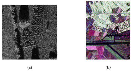
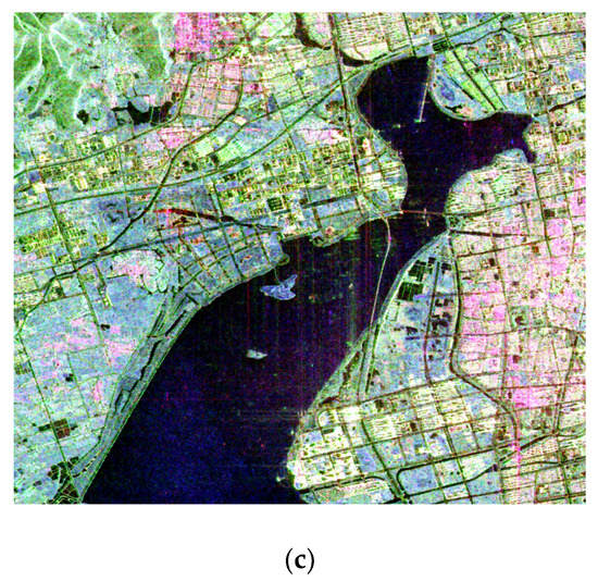
Figure 1.
The experimental datasets: (a) X-band Moving and Stationary Target Recognition (MSTAR) public cluster, Alabama, USA; (b) L-band E-SAR, Oberpfafenhofen, Germany; and (c) C-band GF-3, Suzhou, China.
2.2. Training Samples
Table 1 presents different land cover patches showing significant differences in intensity, texture, structure, etc. Especially for the polarimetric SAR images, single scattering, dihedral scattering, and inclined dihedral scattering introduce huge differences to the feature space. In the VHR (Very High Resolution) airborne SAR image, shrubs and trees have their own distinctive texture features. In this image, the regular stripes make the shrub easy to recognize. For full-polarization SAR images, polarimetric decomposition provides significant benefits for classifying different land cover types. The building area shows a series of linear stripes with a mix of pink and silver colors formed by different heights of inclined dihedral scattering with a certain rotation. The water area is composed of single scattering with a speckle blue color. Other land types also present significant differences. The training samples of the three given datasets are presented in Table 2. For deep models, the imbalance in the quantity of different land types will lead to poor generalization performance and overfitting. To avoid these issues, random elimination was used to ensure the overall balance of training samples. In each training period, the datasets were randomly divided into training and validation sets according to a 4:1 ratio. The test set for each experimental region is the whole SAR image apart from the selected training and validation sets.

Table 1.
Synthetic aperture radar (SAR) patches of different land cover types in the given datasets.
Table 2.
Number of training samples in the three datasets.
3. Methods
3.1. Overall Pipeline for SAR Image Classification
The overall algorithm framework for SAR image classification is presented in this section. The proposed classification algorithm is based on an improved, fully connected CRF model which mainly consists of unary potential function, pairwise potential function, superpixel region constraints, model inference, and parameter optimization. In our proposed approach, the unary potential function is defined by the CNN model, which helps realize patch-based pre-classification to model the single-valued dependency relationship between the observation field and the label field. The linear combination of Gaussian kernels determined the pairwise potential function, which enabled the efficient application of contextual information for sophisticated SAR images. Furthermore, to partially mitigate some of the over-smoothing effect, the superpixel region constraints were integrated into the conventional CRF model. Finally, the mean field approximation inference (MFAI) algorithm was introduced to enable rapid model solving. The overall framework for SAR image classification is depicted in Figure 2.
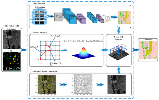
Figure 2.
Overall framework for SAR image classification.
3.2. Fully Connected Conditional Random Field Mode
The conditional random field is a probabilistic graphical model that directly models the posteriori probability of the label field based on observation field. Considering the neighborhood structure of the CRF pairwise potential, the connection types included 4-adjacent, 8-adjacent, and full connection. Compared with the partially connected CRF, the fully connected CRF performed better in the synthesis of global contextual information. It completely perceived shape, texture, and intensity. According to Hammersley–Clifford theorem, the posteriori probability of CRF model is defined as a Gibbs distribution:
where X is the observation field; Y is the label field; ϕc is a potential function defined in the maximum clique c; C is the set of maximum cliques, which is defined in the graph of the label field; and Z(X) is defined as the normalized term. The CRF model aims to infer the MAP label y* for the observed value, which can be represented as follows:
The Gibbs energy for a single label is computed as follows:
For the second-order fully connected CRF model, the Gibbs energy consists of unary potential and pairwise potential. In this case, the posteriori probability of CRF model can be given by the following:
where Σφμ(yi|X) is the unary potential, which represents the per-pixel inference between the observation field and the label field. The unary potential is obtained by the pattern recognition classifier based on each pixel. Σφp(yi,yj|X) is the pairwise potential which describes the correlation among different pixels. The pairwise potential is defined as the linear combination of Gaussian kernels, which is defined as follows:
where μ(yi,yj) is the compatibility function. It is a penalty coefficient for the adjacent similar pixels with different labeling. w(m) is the linear combination weight for the Gaussian kernel k(m)(vi,vj). The Gaussian kernel function is given by the following:
For SAR image classification, the discriminative texture features usually involve the synthesis of multiple intensities and positions [14]. Especially for the polarized SAR data, the operation of polarimetric decomposition introduces multidimensional scattering intensity vectors. Therefore, the pairwise potential is composed of dual Gaussian kernels, which focus on the nearby similar regions and speckle regions, respectively. The two-part Gaussian kernels are defined as follows:
where pi and pj are the pixel positions, Ii and Ij are the intensity vectors, θα and θγ control the degree of nearness, and θβ describes the constraint of similarity. In this two-part Gaussian kernels, the first part dominates the same labeling among similar nearby pixels, and the other helps reduce isolated speckled regions.
The MAP solution of a fully connected CRF model is an inferential optimization. It is a difficult task with high time complexity. Therefore, many algorithms adopt indirect approaches to attain the approximate solution. One of the most efficient algorithms is called filter-based mean field approximation (MFA) inference [39]; it is a variational approximate method based on a series of independent marginal distributions and Gaussian filtering message passing. The mean field algorithm proposes an alternative distribution Q(Y) to replace the original distribution P(Y). This strategy transforms the exact distribution into a series of independent marginals:
This procedure is implemented by minimizing the KL-divergence D(Q||P) between the approximate distribution Q and the original distribution P. The iterative update equation is computed as follows:
where C is the set of cliques on the whole graph and yc is the set of samples in the clique c. For the unary potential, the update equation is extracted as follows:
With regard to the pairwise potential, the update equation is given by the following:
The second-order iterative update equation can be represented as follows:
As for the fully connected CRF model, the computation is still costly in a direct pipeline. To further accelerate the inference, a Gaussian bilateral filter is introduced to realize the efficient computation. The convolution operator with high-dimensional filtering kernels is computed as follows:
where Gm is the mth Gaussian kernel in the pairwise potential and ⊗ is the convolutional operator. For each pixel, the final labeling is determined by the maximum marginal distribution.
| Algorithm 1. Mean field approximation inference. |
| Input: Observation field X and label field Y. The orders of potential function M, the set of maximum clique C, and the number of iterations D. i, j∈[1,…, N], N is the number of samples in a given clique. l∈[l1,…, L], L is the set of labels. |
| 1: Initialize marginal distribution: . |
| 2: While iteration ≤ D do |
| 3: ∀m∈[1, M], i, j∈[1, N] and i ≠ j, compute . |
| 4: Compute . |
| 5: Compute . |
| 6: For all i∈[1, N], normalize . |
| 7: end while |
| Output: The mean field approximation distribution . |
3.3. Convolutional Neural Network Pre-Classification
Compared with conventional pattern recognition algorithms, the convolutional neural network is superior in several advanced aspects, such as big data processing, feature self-learning, and robust generalization. It is more accurate in many pattern-recognition applications [29,40,41,42]. As for the two-order fully connected CRF model, the unary potential needs to acquire an initial labeling probability vector for each single pixel. This is the fundamental pixelwise relation model between the observation and label fields. Therefore, it is advisable for the CRF to fully use the patch-based CNN model as the unary potential. This strategy can offer a superior label probability vector for each sample and can help to relieve the edge-preserving limitation of a patch-based CNN model. As a powerful nonlinear prediction model, the patch-based CNN algorithm has a competitive advantages in local pattern recognition for SAR images. It can provide superior labeling probability vectors [Y1, Y2, Y3,…, Yn] for each pixel, which is suitable as the initial unary potential φμ(yi|X) for the CRF model.
In the convolutional neural topology, multidimensional imagery patterns with complicated texture can be decomposed into hierarchical feature maps. These feature maps provide considerable advantages in terms of descriptive capability and spatial invariance. The powerful feature representation makes this layer-wise connecting network a suitable candidate for the pattern recognition of complex SAR images. There are four main layers in the CNN hierarchy: convolution, pooling, dense connection, and SoftMax. The stacked convolution and pooling layers are the important feature extractors. The dense layers help to reduce feature dimensions. At last, the SoftMax classifier realizes label prediction.
The convolution layer is the important feature extractor. It sets a series of trainable convolutional kernels to extract feature maps. The competitive advantages of the convolution layers lie in the local perceptive fields and weight sharing. These strategies help to efficiently reduce the time and space complexity. Compared with classical fully connected neural networks, the convolution operation takes into account the preservation of spatial locality. In the process of convolutional computation between two layers, the data flows of feature maps follow the following formula:
where f (·) is the activation function, xlj denotes the jth feature map in the lth layer, Mj stands for the sequence of associated features, and klij is a trainable kernel that involves the ith input feature map and the jth output feature map. Through this layer-wise mechanism, multiscale imagery features are converted to advanced abstraction.
Maxpooling is an efficient downsampling operation between different convolution layers. It is used to extract the local patch maximum among neighboring pixels. This layer is able to achieve feature dimension reduction and to improve some degrees of distortion invariance. Maxpooling is represented as follows:
where G denotes the neighboring scale of pooling with offset location (Δx, Δy) and s is the pooling stride. In practical use, we usually adopt the neighboring 2 × 2 with a stride 2 maxpooling.
The dense layer is also called the fully connected layer. In this layer, each neural node is linked to all nodes of the previous layer. It can map multidimensional feature space to a one-dimensional vector. This layer plays an important role in the synthesized representation of hierarchical features. Furthermore, the synthesis of feature weighting also benefits greatly in follow-on regression. The SoftMax model is an extension of the classical logistic regression. It produces perfect performance on multi-class pattern recognition jointly with the CNN topology. The SoftMax model is defined as follows:
where yli denotes the ith labeling prediction vector and al is defined as al = kTxl + b. In addition, xli is the ith input of the lth layer and Σea is a normalization which calculates the weighted sum of all neurons in the lth layer. In the training stage, cross entropy is introduced as the cost function to evaluate the convergent performance. The cross-entropy function is represented as follows:
where yj denotes the label truth of the jth sample, which has been declared in the training dataset. CNN models adopt a backpropagation mechanism to perform the weight update. The gradient of cost function is given by the following:
Depending on i and j, the derivative of cost function is divided into two cases. When i = j, the equation is defined as follows:
Otherwise, the partial differential equation is as follows:
Therefore, the overall gradient of cost function is computed as:
Based on the stochastic gradient descent (SGD) algorithm, the model weights will be updated iteratively. Simply put, backpropagation introduces an efficient control mechanism for feedback in the neural network.
| Algorithm 2. Pre-classified labeling observation field using a convolutional neural network. |
| Input: Training dataset D = {(x1,y1),(x2,y2),…,(xm,ym)}, where x and y denote the data and label, respectively. The number of convolutional layers L, the number of dense layers F, learning rate ε, training epoch M, and batch number B, which divides the dataset into B equal parts {(X1,Y1),(X2,Y2),…,(XB,YB)}. |
| 1: Initialize the convolutional parameter space {μ1, μ2,…, μL}. |
| 2: while training epoch M do |
| 3: for b = 1 to B do |
| 4: Initialize x0b←Xb. |
| 5: for i = 1 to L do |
| 6: Compute using Equation (14). |
| 7: Compute using Equation (15). |
| 8: end for |
| 9: Define . |
| 10: for j = 1 to F do |
| 11: Compute . |
| 12: end for |
| 13: Compute SoftMax function . |
| 14: Compute cost function . |
| 15: Back propagation based on gradient . |
| 16: end for |
| 17: end while |
| Output: Pre-classified observation field. |
3.4. Simple Linear Iterative Clustering Superpixel Boundary Constraint
The two-order fully connected CRF model takes into full consideration the contextual information in image labeling. Simultaneously, the pairwise penalty factor introduces excessive smoothing to the boundaries or narrow micro-regions of the given imagery. To partially alleviate these limitations, the boundary constraint mechanism is integrated into the model inference. A superpixel is a small irregular imagery patch with self-similar visual sense in terms of intensity and texture. It is an efficient simplified representation of a complex observation field. Therefore, it has the potential to provide a boundary constraint for the CRF inference, which aims to alleviate excessive smoothing, to some degree.
The boundaries of all extracted superpixels are regarded as auxiliary decision-making information for the CRF inference framework. This mechanism provides a beneficial modification that improves the whole model. In fact, it further strengthens the associated dependency among the pixel neighborhood. In order to introduce the boundary constraint, Equation (12) is followed by a weighted computation. For pixel i, the weighted formula is defined as follows:
where ws is the constrained weight. Pixel i is located in the superpixel region Si, and the number of pixels in Si is given by Ni. In the iterative process of CRF inference, the posteriori probability of each pixel is modified by the average probability in the boundary constraint region.
Many researches have been looking forward toward graph-cut algorithms having great potential in improving SAR image classification [16,18]. The simple linear iterative clustering (SLIC) algorithm [43] is a state-of-the-art graph-cut method. It adopts the idea of space transformation and clustering to generate a series of highly self-similar superpixels. This algorithm supports the graph-cut of color and gray images. Therefore, it is suitable for processing single and full polarization SAR images. The SLIC algorithm has competitive advantages in generating ideal boundary constraints for the random field inference procedure. Firstly, the computational cost of the SLIC optimization is dramatically reduced by limiting the searching space. This reduces the space complexity to linear. On the other hand, the synthesis of distance measures combines intensity and spatial proximity, which offers an efficient approach to controlling the size and compactness of superpixels. In this graph-cut algorithm, the single pixel is transformed into a feature vector Pi = [li ai bi xi yi]T, including the CIELAB (Commission Internationale de l’Eclairage lab value) color space and location coordinates. [li ai bi] is the vector of CIELAB color space. li is the value of lightness. ai and bi are the complementary intensity values. [xi yi] stand for the position of the image pixel. The feature vector Pi expands the conventional pixel representation. The single pixel is represented as a comprehensive vector combined with position and multiple intensity spaces. The distance measure of different pixels is given by the following:
where dc is the distance of the color space, ds is the distance of the location space, and NC and NS are the color and location normalization, respectively. This distance measure is the evaluation criteria for later clustering. The initially given cluster centers are adjusted iteratively according to the nearest distance D. Comparing the latter with the former cluster centers, the residual error E is computed by an L2 normalization. The stepwise update is performed until the residual error converges.
| Algorithm 3. The mean field approximation inference (MFAI) superpixel boundary constraint. |
| Input: The MFA distribution Q in each inference iteration, the superpixel boundary S, the number of pixels in each superpixel N, the constrained weight of superpixel boundary ws. 1: for each MFAI iteration do |
| 2: for each pixel in the identical superpixel Si do |
| 3: Compute superpixel average probability . |
| 4: Iterative compute and weighted update . |
| 5: end for |
| 6: Initialize . |
| 7: end for |
| Output: The CRF probability distribution with superpixel boundary constraint. |
4. Experimental Results
In this part, we designed a series of contrast experiments to verify the validity of our proposed classification algorithm. Several widely used features and machine learning algorithms were introduced to the contrast evaluation. In the contrast experiments, we adopted different hand-designed features that are accepted as state-of-the-art methods for SAR image classification, including GLCM and Gabor wavelet. In addition, multiple widely accepted machine learning algorithms were involved in the controlled experiments, including SVM, RF, GBDT, baseline CNN, and ConvCRF. In order to guarantee statistically significant experiments and to acquire average results, the Monte Carlo random state and data shuffle strategy were introduced to the multiple redundancy-repeating runs. Each independent run used a random data queue and model initial state. Reasonable adjustment of hyperparameters was conducted to ensure convergence and efficiency of the different involved classification algorithms.
In the final accuracy evaluation stage, we used the average producer’s accuracy (PA), user’s accuracy (UA), overall accuracy (OA), and kappa coefficient as the main assessment indexes. PA denotes the fraction of correctly classified pixels with regard to all pixels of that ground truth class, and UA indicates the fraction of correctly classified pixels with regard to all pixels classified as this class in the classified image. OA is calculated as the total number of correctly classified pixels divided by the total number of test pixels. The kappa coefficient represents the agreement between the classification result and the ground truth, which ranges from 0 to 1. The closer this value is to 1, the higher accuracy the classification is.
4.1. Classification Experiments on MSTAR X-Band Single-Polarized Dataset
The MSTAR cluster is a public open dataset with 0.3-m resolution and single polarization. In this experiment, multiple algorithms with optimal hyperparameters were adopted to perform controlled contrast experiments. The Monte Carlo random state and data shuffle training strategies were introduced to duplicate the experiment multiple times and to figure out statistically average results. The classification maps of the involved algorithms and the accuracy statistics are displayed in Figure 3 and Table 3.
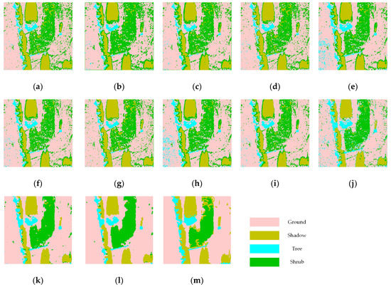
Figure 3.
Classification maps of involved algorithms on the MSTAR data: (a) gray + support vector machine (SVM); (b) gray + random forest (RF); (c) gray + gradient boosting decision tree (GBDT); (d) gray + Gabor + SVM; (e) gray + Gabor + RF; (f) gray + Gabor + GBDT; (g) gray + GLCM + SVM; (h) gray + GLCM + RF; (i) gray + GLCM + GBDT; (j) baseline convolutional neural network (CNN); (k) ConvCRF; (l) our algorithm; and (m) ground truth.
Table 3.
Accuracy comparison of classification on MSTAR dataset.
It is intuitively depicted in Figure 3 that the speckle noise widely distributed in VHR single-polarized SAR images has extremely negative effects on the classification tasks. According to Figure 3, it is noticeable that the classification maps of the SVM, RF, GBDT, and baseline CNN algorithms are seriously polluted by the misclassified speckle points. As for the inherent backscattering features, most of the fuzzy classification confusion is distributed in shrub and ground areas. After the GLCM and Gabor wavelet texture representations were introduced to combine the inherent backscattering and hand-designed features, obviously, the classification results were partially improved in the former confusing areas. Furthermore, it can be illustrated that the edges of different land cover types exhibit many misclassified commission errors, especially in the boundary of radar shadow and ground areas. The baseline CNN algorithm improved the pattern recognition of different land cover types and alleviated some of the speckle confusion and boundary errors. Our proposed method presents obvious superiority to the other algorithms. Compared with the other methods, the speckle confusion and boundary error are effectively resolved in our algorithm. Moreover, the SBC mechanism applied to global inference realizes a more complete structure preservation for the boundary of different land cover types.
According to Table 3, we can draw more quantitative conclusions. It can be intuitively noticed that there are significant differences in the classification accuracy of multiple algorithms. Our proposed method achieves better performance than the other models for most land cover types. Especially for the shrub area, the proposed method almost increases the classification producer accuracy by more than 10%. We can infer that the proposed method has more powerful recognition ability for complex texture cover types in SAR images, such as shrubs and trees. In addition, compared with the combination of classical machine learning algorithms and widely accepted hand-designed feature extractors, the deep models present dominant advantages, as evidenced by the OA and kappa coefficient values. However, it is worth noting that the hand-designed features combined with machine learning algorithms provide a partial advantage in shadow extraction. According to the previous analysis, the deep models are less sensitive to homogeneous land types with low backscattering intensity. However, as with the classical machine learning algorithms, this difference is not obvious.
4.2. Classification Experiments on E-SAR L-Band Full-Polarization Dataset
The L-band E-SAR Oberpfafenhofen is a full-polarization SAR data with 3-m resolution. The Pauli-basis decomposition [|SHH+SVV|2, |SHH-SVV|2, 2|SHV|2] based on the polarimetric scattering coherence matrix provides more discriminative information for SAR image classification. In our experiments, several hand-designed texture feature extractors and machine learning algorithms were adopted to perform the comparative tests. All machine learning experiments followed the Monte Carlo runs and data shuffle strategy to acquire statistically average results. The classification maps of the considered algorithms are shown in Figure 4. Moreover, the quantitative accuracy evaluation is displayed in Table 4.
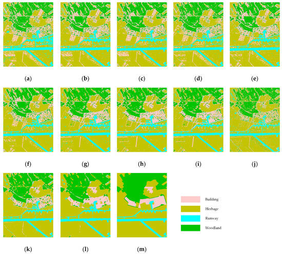
Figure 4.
Classification maps of involved algorithms on the E-SAR data: (a) polar + SVM; (b) polar + RF; (c) polar + GBDT; (d) polar + Gabor + SVM; (e) polar + Gabor + RF; (f) polar + Gabor + GBDT; (g) polar + GLCM + SVM; (h) polar + GLCM + RF; (i) polar + GLCM + GBDT; (j) baseline CNN; (k) ConvCRF; (l) our algorithm; and (m) ground truth.
Table 4.
Accuracy comparison of classification on E-SAR dataset.
As shown in Figure 4, it is worth noting that most of the widely accepted SAR image classification algorithms suffer from serious speckle pollution and boundary confusion. The commission error mainly occurs in building areas, and the omission error is mainly distributed in building and woodland areas. When only using inherent backscattering polarized information to conduct classification tasks, the different land cover types are extremely confused, especially in building areas. After introducing hand-designed texture features, the confusion errors were drastically reduced. However, the boundary between woodland and herbage areas still has many misclassified errors. It is intuitively illustrated that our proposed algorithm provides competitive advantages in the pattern recognition of different land cover types and performs better in terms of the generalization and robustness of the widespread speckle noise. In addition, the proposed method efficiently reduces boundary errors and preserves the complete structure.
Moreover, we can get more quantitative accuracy results in Table 4. It is noticeable is that the proposed algorithm has dominant advantages in the extraction of buildings and woodland. Compared with the widely used algorithms, the proposed method increases the producer accuracy of building and vegetation areas by roughly 10%. The OA and kappa coefficient also display considerable improvement. It is noted that the combination of polarimetric scattering and GLCM texture features also works well in polarized SAR image classification. Similar to what we have observed earlier, the homogenous airport runway area with low scattering intensity is not sensitive to texture descriptors. The scattering features with machine learning algorithms achieve the best performance in terms of the extraction of airport runway.
4.3. Classification Experiments on GF-3 C-Band Full-Polarization Dataset
The GF-3 dataset is a Pauli-basis decomposition SAR image with 8-m resolution. In the experiments with GF-3 data, we adopted multiple machine learning algorithms to evaluate the accuracy, including SVM, RF, GBDT, baseline CNN, ConvCRF, and our proposed algorithm. Furthermore, widely used hand-designed texture descriptors were also introduced to contrast the experiments. All the machine learning algorithms executed Monte Carlo random state and the data shuffle strategy to ensure the independence of repeating runs. The classification maps and accuracy results are presented in Figure 5 and Table 5, respectively.
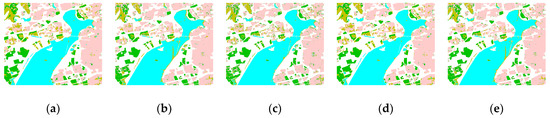
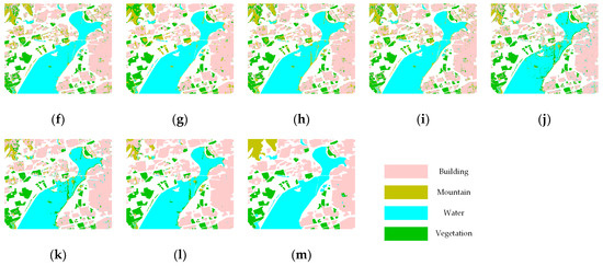
Figure 5.
Classification maps of involved algorithms on the GF-3 data: (a) polar + SVM; (b) polar + RF; (c) polar + GBDT; (d) polar + Gabor + SVM; (e) polar + Gabor + RF; (f) polar + Gabor + GBDT; (g) polar + GLCM + SVM; (h) polar + GLCM + RF; (i) polar + GLCM + GBDT; (j) baseline CNN; (k) ConvCRF; (l) our algorithm; and (m) ground truth.
Table 5.
Accuracy comparison of classification on GF-3 dataset.
According to Figure 5, it is intuitively illustrated that most of involved algorithms achieve good performance on the classification of GF-3 polarimetric SAR data. As for this moderate spatial-resolution SAR image, the negative impact of speckle noise apparently decreased with large-scale pattern recognition of land cover types. Several machine learning algorithms combined with hand-designed texture descriptors performed better on the extraction of water and mountains. However, on account of the lower generalization, their classification maps suffered serious speckle pollution in building and vegetation areas. However, it is worth noting that the proposed method successfully solved this problem. It can realize higher accuracy in building and vegetation areas and produced a cleaner classification map. It is noticeable is that the baseline CNN algorithm was not superior in the classification of this moderate spatial-resolution polarimetric SAR image. It was inferior to the ConvCRF algorithm in the highly fragmented areas.
The complete accuracy evaluation statistics are provided in Table 5 in detail. As shown in Table 5, we can observe that commission errors mainly exists in mountain and vegetation areas, while omission errors were mainly distributed in mountain areas. Compared with state-of-the-art machine learning algorithms, the proposed method achieves a better performance in terms of the OA and kappa coefficient. In addition, it has an obvious advantage in the recognition of buildings and vegetation, which contain more complex texture features with fuzzy speckle noise. Moreover, it is worth noting that the widely accepted machine learning methods achieve higher accuracy in the extraction of water areas.
5. Analysis and Discussion
This section provides our detailed analysis and discussion of the whole experimental pipeline. Section 5.1 discusses the selection of optimal hyperparameters. The effectiveness analysis of the superpixel boundary constraint is illustrated in Section 5.2.
5.1. Selection of Optimal Hyperparameters
The selection of optimal hyperparameters is essential for the final classification performance. In other words, the settings of different hyperparameters have significant impacts on the feature representation, model velocity, and veracity of the results. In our contrast experiments, we set multiple hyperparameters to evaluate different experimental trajectories and to select the optimal values as the final settings. Considering the influence and priority in varying degrees, we selected a series of key parameters, including the size of SAR patches, the computational weights of two-part Gaussian kernels, the intensity factor of the first Gaussian kernel, and the nearness factors of the two-part Gaussian kernels. Moreover, the parameters of the superpixel boundary constraint are also important for the overall model performance, which is analyzed and evaluated in detail in Section 5.2. All our experiments were conducted using the scientific Python development environment on the Windows platform with Intel Core i7-4790K CPU, NVIDIA Tesla K20c GPU, and 32 GB running memory. In addition, an international end-to-end open-source machine learning framework TensorFlow undertook a part of the feature computational work. We introduced a parallel computing library CUDA to accelerate the computing speed.
In this part, we conducted contrast experiments and analyses on the three given datasets. Large coverage and messy mixing regions were included in these typical multi-polarization SAR images, which put forward higher robustness and requirements on algorithm performance. To verify the reliability of the experiments and to exclude accidents, we conducted multiple repeated experiments to acquire the average overall accuracy (OA) and Kappa coefficient. Furthermore, some statistically significant strategies were also used in these machine learning experiments, including Monte Carlo random state and data shuffle.
First, we designed a series of contrast experiments to analyze the patch size setup. Multiple patch scales ranging from 7 to 15 for X-band MSTAR SAR, 5 to 13 for L-band E-SAR, and 19 to 27 for the C-band GF-3 SAR were evaluated with a fixed offset. In Figure 6, it is intuitively observed that SAR patch size has a significant influence on the classification performance. For the identical SAR dataset, varying scales of patch size lead to slight fluctuation in classification accuracy within a certain range. Meanwhile, the classification results of airborne and spaceborne SAR images also showed different sensitivities to patch size. According to the experimental results, the optimal SAR patch sizes of the given datasets are 13, 5, and 25, respectively. Moreover, stepwise accuracy analysis of the proposed model demonstrated differences in algorithm performance. An optimal patch size realizes a classified balance between the degrees of discrimination and confusion, which captures abundant discriminative features and suppresses much of the classification confusion. In Figure 7, the C-band GF-3 polSAR dataset is used as an example. Clearly, it is observed that the classification performance changes with the increase of SAR patch sizes.
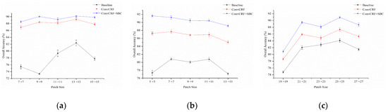
Figure 6.
Statistical results of the overall accuracy (OA) varying with a series of patch sizes for the given datasets: OA of the (a) MSTAR public cluster, (b) E-SAR, and (c) GF-3 datasets for multiscale patch sizes.
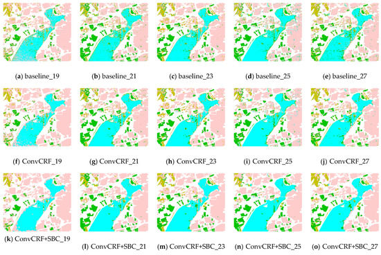
Figure 7.
Sample classification maps of the C-band GF-3 polSAR varying with the increase in patch size from 19 to 27 (offset step = 2): (a–e) The baseline CNN model; (f–j) the proposed model without the superpixel boundary constraint (SBC) mechanism; and (k–o) the proposed model.
In the second setup, we conducted contrast sensibility tests of the hyperparameters for Gaussian kernel functions in our proposed model. Variable hyperparameters of the kernels had a slight effect on the final classification results. In order to explore the sensitivity analysis of Gaussian kernel functions independently and to exclude the training uncertainty of CNN, we controlled the experiments to select the same CNN prediction as unary potential. As a result, for each set of Gaussian kernel parameters, we acquired a unique constant probability graph. In this experiment, OA was only affected by the hyperparameters of Gaussian kernel functions. Therefore, the experimental results had no standard deviation in this part.
The four main hyperparameters that dominated the nearness labeling and speckle reduction were evaluated in this part, including nearby similarity weight, nearness factor, intensity factor, and isolated speckle weight. A sample of the results with the MSTAR dataset is depicted in Figure 8, which shows the change regularity of OA with different parameter settings. In general, these four main kernel function hyperparameters dominated the contextual feature information and speckle noise filtering of the overall model framework. Figure 8a illustrates that OA rises at first and then gradually flattens with increasing nearby similarity weight. Variable nearness factors in the first kernel also have different effects on OA. The larger nearness factors in the first kernel are more efficient at improving OA, but they are not sensitive to nearby similarity weight. Figure 8b depicts the dynamic factor relationship in the first kernel. Although these two factors make small differences in the absolute OA value, given the inverse relationship between computational factors and signal intensity, we infer that the nearness factor has a relatively larger impact on OA. Moreover, we can see a more significant relation between the nearness factors and the isolated speckle weights in Figure 8c. For the smaller nearness factors in the second kernel, OA is not sensitive to the isolated speckle weight. Meanwhile, with the increasing of nearness factor in the second kernel, the proposed model has better performance at first and then shows an obvious decrease.
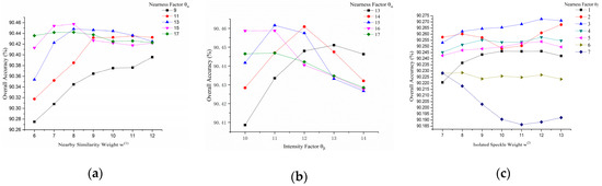
Figure 8.
The sample sensibility tests of hyperparameters for Gaussian kernel functions on the MSTAR dataset: OA varying with (a) nearby similarity weights and nearness factors, (b) intensity and nearness factors, and (c) isolated speckle weights and nearness factors.
5.2. Effectiveness Analysis of SBC
In this part, we used the MSTAR data as an example to analyze the effectiveness of the SBC mechanism in SAR image classification. Although the ConvCRF model performed better than the baseline deep learning model, MFAI still introduced excessive smoothing omission error to imaging boundaries or narrow micro-regions. To partially mitigate this issue, the SBC mechanism was applied to the MFAI iterative computing process to minimize the labeling loss of the classical unconstrained inference. In this part, we focus on a discussion of the effect of different SBC hyperparameters. The main constraint factors that control homogeneity and edges are the number of super cliques and adjacent compaction. In this experiment, OA was only affected by the parameters of SBC. As for the same SBC parameter setting, the classification result is invariable. Therefore, the experimental results had no standard deviation in this part. In Figure 9, we present a series of stepwise SBC conditions. Moreover, to give a visual display of the SBC regions, the pixels within identical iterative computing boundaries were replaced by the mean values. It is worth noting that the homogeneous edges were found to be strongly influenced by the quantity and compaction factors in the high-resolution cluster SAR image. In addition, we can observe that the micro-regions and edges of the sample classification maps were influenced by the different SBC parameters. Figure 10a illustrates that the hyperparameters of SBC have an obvious influence on OA. With the increasing number of superpixels, OA rose up at first and then gradually decreased in most cases. If it was below the optimal scale, the clique was too small to obtain a precise edge. The excessively large scale introduced considerable confusion instead. On the other hand, we introduced different constrained levels of the SBC mechanism in the MFAI process. Variable constraint weights are involved in the MFAI computing procedure. The experimental results of different SBC controlling powers are presented in Figure 10b. As the constraint weight increased, OA showed an approximately single-peak distribution.
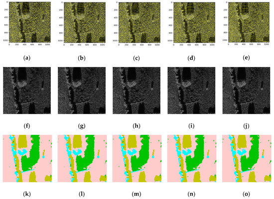
Figure 9.
Boundary constraint conditions with varying numbers of superpixels: (a–e) ConvCRF boundary constraint maps with superpixels ranging from 1500 to 2300. (step size = 200); (f–j) corresponding mean maps of the MFAI regions; and (k–o) corresponding MFAI classification maps of the proposed models with different SBC parameters.
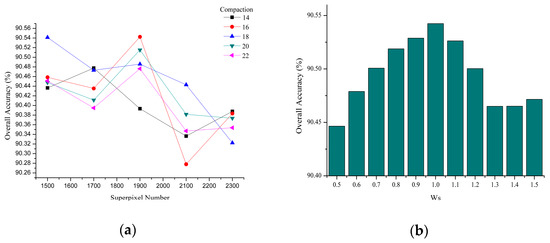
Figure 10.
The sample sensibility test of SBC: (a) OA varying with the number of superpixels and compaction and (b) OA varying with the constraint weight.
5.3. Sensitivity Analysis of Increasing Data Portions
Generally speaking, the conventional single-stream deep models need large datasets to ensure the generalization ability. Our proposed method combined CRF with deep model and SBC mechanism. In this part, we put forward exploratory motivation to analyze the sensitivity and robustness with respect to the increasing training dataset portion. In our experiments, we performed dozens of runs on the proposed model using only 10% of the whole datasets and then by randomly increasing by 10% from the rest of the dataset at a time. In Figure 11, it is intuitively observed that OA rises up with the increase in dataset portion. Furthermore, the growth of OA gradually changes slowly. Compared with the proposed model, the baseline CNN is more subjected to the increase in dataset portion. Moreover, it is worth noting that the different image sizes and polarization also present different sensitivities to the increase in dataset portion. Figure 12 and Figure 13 display classification maps of E-SAR data using baseline CNN and our proposed model with 10% dataset portion increase at a time. It is proven that the proposed model has better performance on robustness with respect to the increasing training dataset portion.
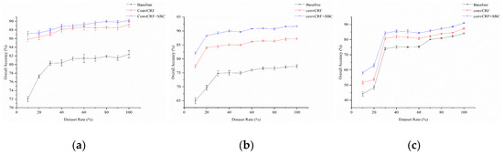
Figure 11.
OA varying with the increase of dataset portion: OA of the (a) MSTAR public cluster, (b) E-SAR, and (c) GF-3 datasets with 10% increases at a time.
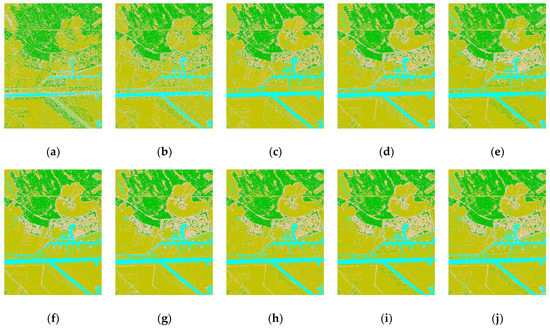
Figure 12.
Classification maps of E-SAR data using the baseline CNN model with increasing dataset portions: (a–j) dataset portions ranging from 10% to 100% and 10% increases at a time.
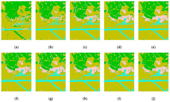
Figure 13.
Classification maps of E-SAR data using our proposed model with increasing dataset portions: (a–j) dataset portions ranging from 10% to 100% and 10% increases at a time.
6. Conclusions
High-resolution SAR image classification is always a challenging topic in the fundamental research of microwave remote sensing. In this paper, a novel integrated learning algorithm using ConvCRF with the SBC mechanism was proposed for single and full polarization SAR image classification. According to a series of systematic verifications of contrast experiments, it is clear that the proposed algorithm can successfully obtain optimized classification maps and higher accuracy indexes. The proposed algorithm combines local feature representation with the global MFAI process, which can effectively relieve the issues of confusing speckle noise and can promote local pattern recognition in high-resolution SAR images. In the land cover classification experiments using the MSTAR, E-SAR, and GF-3 datasets, the overall accuracy of our proposed method achieves 90.18 ± 0.37, 91.63 ± 0.27, and 90.91 ± 0.31, respectively. In addition, it is worth noting that the proposed method provides competitive advantages in the classification of building and woodland areas, which has potential for remote sensing analysis of urban and agricultural applications. Additionally, for the shrub area in the MSTAR data, the proposed method almost increased the classification producer accuracy by more than 10%. The proposed method presents better performance on the representation of dense texture features. However, compared with other machine learning algorithms with widely used texture descriptors, the proposed algorithm still has some aspects that remain to be improved, especially in terms of homogeneous land cover types with low backscattering intensity. The contrast experiments conducted on different microwave bands of airborne and spaceborne SAR images also verified the applicability of our algorithm.
In order to improve the intelligent analysis of SAR images for more comprehensive remote sensing applications, follow-up research could focus on a wide range of aspects, including ensemble learning with multiple algorithms, more flexible and independent learning with a lower degree of supervision, greedy learning from large amounts of SAR patches, the more efficient patch-scale learning with prior knowledge and mathematical morphology.
Author Contributions
Conceptualization, Z.S., M.L., P.L., J.L., T.Y. and X.G.; methodology, Z.S. and P.L.; investigation and data acquisition, Z.S., M.L., Z.Z., J.L., J.Y., X.M. and W.C.; data analysis and original draft preparation, Z.S., M.L., T.Y. and X.G.; validation, Z.S. and M.L.; writing and review, Z.S., M.L., T.Y. and X.G.; funding acquisition, T.Y. and X.G. All authors have read and agreed to the published version of the manuscript.
Funding
This research was funded by the National Key R&D Program of China “Research on establishing medium spatial resolution spectrum earth and its application”, China’s 13th Five-year Plan Civil Space Pre-Research Project under grant Y7K00100KJ, and China’s 13th Five-year Plan Civil Space Pre-Research Project “National emergency planning, response and information support using satellite remote sensing” under grant Y930060K8M.
Acknowledgments
The authors would like to thank the associate editor and anonymous reviewers for their helpful and constructive suggestions. The authors also thank the National Demonstration Center of Spaceborne Remote Sensing for their generous provision of GF-3 SAR images.
Conflicts of Interest
The authors declare no conflict of interest.
References
- Moreira, A.; Prats-Iraola, P.; Younis, M.; Krieger, G.; Hajnsek, I.; Papathanassiou, K.P. A tutorial on synthetic aperture radar. IEEE Geosci. Remote Sens. Mag. 2013, 1, 6–43. [Google Scholar] [CrossRef]
- Mori, S.; Polverari, F.; Mereu, L.; Pulvirenti, L.; Montopoli, M.; Pierdicca, N.; Marzano, F.S. Atmospheric precipitation impact on synthetic aperture radar imagery: Numerical model at X and KA bands. In Proceedings of the 2015 IEEE International Geoscience and Remote Sensing Symposium (IGARSS), Milan, Italy, 26–31 July 2015. [Google Scholar]
- Singha, S.; Johansson, M.; Hughes, N.; Hvidegaard, S.M.; Skourup, H. Arctic Sea Ice Characterization Using Spaceborne Fully Polarimetric L-, C-, and X-Band SAR with Validation by Airborne Measurements. IEEE Trans. Geosci. Remote Sens. 2018, 56, 3715–3734. [Google Scholar] [CrossRef]
- Nunziata, F.; Gambardella, A.; Migliaccio, M. On the Mueller Scattering Matrix for SAR Sea Oil Slick Observation. IEEE Geosci. Remote Sens. Lett. 2008, 5, 691–695. [Google Scholar] [CrossRef]
- Krestenitis, M.; Orfanidis, G.; Ioannidis, K.; Avgerinakis, K.; Vrochidis, S.; Kompatsiaris, I. Oil Spill Identification from Satellite Images Using Deep Neural Networks. Remote Sens. 2019, 11, 1762. [Google Scholar] [CrossRef]
- Bai, Y.; Gao, C.; Singh, S.; Koch, M.; Adriano, B.; Mas, E.; Koshimura, S. A Framework of Rapid Regional Tsunami Damage Recognition from Post-event TerraSAR-X Imagery Using Deep Neural Networks. IEEE Geosci. Remote Sens. Lett. 2018, 15, 43–47. [Google Scholar] [CrossRef]
- Brunner, D.; Lemoine, G.; Bruzzone, L. Earthquake Damage Assessment of Buildings Using VHR Optical and SAR Imagery. IEEE Trans. Geosci. Remote Sens. 2010, 48, 2403–2420. [Google Scholar] [CrossRef]
- Dumitru, C.O.; Schwarz, G.; Datcu, M. SAR Image Land Cover Datasets for Classification Benchmarking of Temporal Changes. IEEE J. Sel. Top. Appl. Earth Obs. Remote Sens. 2018, 11, 1571–1592. [Google Scholar] [CrossRef]
- Antropov, O.; Rauste, Y.; Astola, H.; Praks, J.; Häme, T.; Hallikainen, M.T. Land Cover and Soil Type Mapping from Spaceborne PolSAR Data at L-Band with Probabilistic Neural Network. IEEE Trans. Geosci. Remote Sens. 2014, 52, 5256–5270. [Google Scholar] [CrossRef]
- Sun, Z.; Li, J.; Liu, P.; Cao, W.; Yu, T.; Gu, X. SAR Image Classification Using Greedy Hierarchical Learning with Unsupervised Stacked CAEs. IEEE Trans. Geosci. Remote Sens. 2020, 1–19. [Google Scholar] [CrossRef]
- Kurosu, T.; Fujita, M.; Chiba, K. Monitoring of rice crop growth from space using the ERS-1 C-band SAR. IEEE Trans. Geosci. Remote Sens. 1995, 33, 1092–1096. [Google Scholar] [CrossRef]
- Lopez-Sanchez, J.M.; Cloude, S.R.; Ballester-Berman, J.D. Rice Phenology Monitoring by Means of SAR Polarimetry at X-Band. IEEE Trans. Geosci. Remote Sens. 2012, 50, 2695–2709. [Google Scholar] [CrossRef]
- Maillard, P.; Clausi, D.A.; Huawu, D. Operational map-guided classification of SAR sea ice imagery. IEEE Trans. Geosci. Remote Sens. 2005, 43, 2940–2951. [Google Scholar] [CrossRef]
- Dai, D.; Yang, W.; Sun, H. Multilevel Local Pattern Histogram for SAR Image Classification. IEEE Geosci. Remote Sens. Lett. 2011, 8, 225–229. [Google Scholar] [CrossRef]
- Fletcher, N.D.; Evans, A.N. Minimum distance texture classification of SAR images using wavelet packets. In Proceedings of the IEEE International Geoscience and Remote Sensing Symposium, Toronto, ON, Canada, 24–28 June 2002. [Google Scholar]
- Geng, J.; Wang, H.; Fan, J.; Ma, X. Deep Supervised and Contractive Neural Network for SAR Image Classification. IEEE Trans. Geosci. Remote Sens. 2017, 55, 2442–2459. [Google Scholar] [CrossRef]
- Chen, S.; Wang, H.; Xu, F.; Jin, Y. Target Classification Using the Deep Convolutional Networks for SAR Images. IEEE Trans. Geosci. Remote Sens. 2016, 54, 4806–4817. [Google Scholar] [CrossRef]
- Ren, Z.; Hou, B.; Wen, Z.; Jiao, L. Patch-Sorted Deep Feature Learning for High Resolution SAR Image Classification. IEEE J. Sel. Top. Appl. Earth Obs. Remote Sens. 2018, 11, 3113–3126. [Google Scholar] [CrossRef]
- Geng, J.; Wang, H.; Fan, J.; Ma, X. Change detection of SAR images based on supervised contractive autoencoders and fuzzy clustering. In Proceedings of the 2017 International Workshop on Remote Sensing with Intelligent Processing (RSIP), Shanghai, China, 19–21 May 2017. [Google Scholar]
- Guo, Y.; Sun, Z.; Qu, R.; Jiao, L.; Liu, F.; Zhang, X. Fuzzy Superpixels Based Semi-Supervised Similarity-Constrained CNN for PolSAR Image Classification. Remote Sens. 2020, 12, 1694. [Google Scholar] [CrossRef]
- Rostami, M.; Kolouri, S.; Eaton, E.; Kim, K. Deep Transfer Learning for Few-Shot SAR Image Classification. Remote Sens. 2019, 11, 1374. [Google Scholar] [CrossRef]
- Tin Kam, H. The random subspace method for constructing decision forests. IEEE Trans. Pattern Anal. Mach. Intell. 1998, 20, 832–844. [Google Scholar] [CrossRef]
- Chang, C.C.; Lin, C.J. LIBSVM: A library for support vector machines. ACM Trans. Intell. Syst. Technol. 2011, 2, 27. [Google Scholar] [CrossRef]
- Breiman, L. Random Forests; Kluwer Academic Publishers: Dordrecht, The Netherlands, 2001; pp. 5–32. [Google Scholar]
- Friedman, J. Greedy Function Approximation: A Gradient Boosting Machine. Ann. Stat. 2000, 29, 1189–1232. [Google Scholar] [CrossRef]
- Vincent, P.; Larochelle, H.; Bengio, Y.; Manzagol, P.-A. Extracting and composing robust features with denoising autoencoders. In Proceedings of the 25th international conference on Machine learning, Helsinki, Finland, 5–9 July 2008. [Google Scholar]
- Lecun, Y.; Bottou, L.; Bengio, Y.; Haffner, P. Gradient-based learning applied to document recognition. Proc. IEEE 1998, 86, 2278–2324. [Google Scholar] [CrossRef]
- Hinton, G.E.; Osindero, S.; Teh, Y.-W. A Fast Learning Algorithm for Deep Belief Nets. Neural Comput. 2006, 18, 1527–1554. [Google Scholar] [CrossRef] [PubMed]
- Goodfellow, I.J.; Pouget-Abadie, J.; Mirza, M.; Xu, B.; Warde-Farley, D.; Ozair, S.; Courville, A.; Bengio, Y. Generative adversarial nets. In Proceedings of the 27th International Conference on Neural Information Processing Systems—Volume 2, Montreal, QC, Canada, 8–13 December 2014. [Google Scholar]
- Chen, L.; Papandreou, G.; Kokkinos, I.; Murphy, K.; Yuille, A.L. DeepLab: Semantic Image Segmentation with Deep Convolutional Nets, Atrous Convolution, and Fully Connected CRFs. IEEE Trans. Pattern Anal. Mach. Intell. 2018, 40, 834–848. [Google Scholar] [CrossRef]
- Zheng, S.; Jayasumana, S.; Romera-Paredes, B.; Vineet, V.; Su, Z.; Du, D.; Huang, C.; Torr, P.H.S. Conditional Random Fields as Recurrent Neural Networks. In Proceedings of the 2015 IEEE International Conference on Computer Vision (ICCV), Las Condes, Chile, 11–18 December 2015. [Google Scholar]
- Dumitru, C.O.; Schwarz, G.; Cui, S.; Datcu, M. Improved image classification by proper patch size selection: TerraSAR-X vs. Sentinel-1A. In Proceedings of the 2016 International Conference on Systems, Signals and Image Processing (IWSSIP), Bratislava, Slovakia, 23–25 May 2016. [Google Scholar]
- Tabti, S.; Deledalle, C.; Denis, L.; Tupin, F. Patch-based SAR image classification: The potential of modeling the statistical distribution of patches with Gaussian mixtures. In Proceedings of the 2015 IEEE International Geoscience and Remote Sensing Symposium (IGARSS), Milan, Italy, 26–31 July 2015. [Google Scholar]
- Huang, B.; Zhao, B.; Song, Y. Urban land-use mapping using a deep convolutional neural network with high spatial resolution multispectral remote sensing imagery. Remote Sens. Environ. 2018, 214, 73–86. [Google Scholar] [CrossRef]
- Picco, M.; Palacio, G. Unsupervised Classification of SAR Images Using Markov Random Fields and G0 Model. IEEE Geosci. Remote Sens. Lett. 2011, 8, 350–353. [Google Scholar] [CrossRef]
- Zhang, P.; Li, M.; Wu, Y.; Li, H. Hierarchical Conditional Random Fields Model for Semisupervised SAR Image Segmentation. IEEE Trans. Geosci. Remote Sens. 2015, 53, 4933–4951. [Google Scholar] [CrossRef]
- Krähenbühl, P.; Koltun, V. Efficient inference in fully connected CRFs with Gaussian edge potentials. In Proceedings of the 24th International Conference on Neural Information Processing Systems, Granada, Spain, 12–15 December 2011. [Google Scholar]
- Keydel, E.; Lee, S.; Moore, J. MSTAR extended operating conditions—A tutorial. Proc. SPIE Int. Soc. Opt. Eng. 1996, 2757, 228–242. [Google Scholar]
- Vineet, V.; Warrell, J.; Torr, P.H.S. Filter-Based mean-field inference for random fields with higher-order terms and product label-spaces. In Proceedings of the 12th European conference on Computer Vision—Volume Part V, Florence, Italy, 7–13 October 2012. [Google Scholar]
- Krizhevsky, A.; Sutskever, I.; Hinton, G.E. ImageNet classification with deep convolutional neural networks. In Proceedings of the 25th International Conference on Neural Information Processing Systems—Volume 1, Lake Tahoe, Nevada, 3–6 December 2012. [Google Scholar]
- LeCun, Y.; Bengio, Y.; Hinton, G. Deep learning. Nature 2015, 521, 436–444. [Google Scholar] [CrossRef]
- Ren, S.; He, K.; Girshick, R.; Sun, J. Faster R-CNN: Towards Real-Time Object Detection with Region Proposal Networks. IEEE Trans. Pattern Anal. Mach. Intell. 2017, 39, 1137–1149. [Google Scholar] [CrossRef]
- Achanta, R.; Shaji, A.; Smith, K.; Lucchi, A.; Fua, P.; Süsstrunk, S. SLIC Superpixels Compared to State-of-the-Art Superpixel Methods. IEEE Trans. Pattern Anal. Mach. Intell. 2012, 34, 2274–2282. [Google Scholar] [CrossRef] [PubMed]


Publisher’s Note: MDPI stays neutral with regard to jurisdictional claims in published maps and institutional affiliations. |
© 2021 by the authors. Licensee MDPI, Basel, Switzerland. This article is an open access article distributed under the terms and conditions of the Creative Commons Attribution (CC BY) license (http://creativecommons.org/licenses/by/4.0/).