Cluster-Wise Weighted NMF for Hyperspectral Images Unmixing with Imbalanced Data

Abstract

Hyperspectral unmixing is an important technique for analyzing remote sensing images which aims to obtain a collection of endmembers and their corresponding abundances. In recent years, non-negative matrix factorization (NMF) has received extensive attention due to its good adaptability for mixed data with different degrees. The majority of existing NMF-based unmixing methods are developed by incorporating additional constraints into the standard NMF based on the spectral and spatial information of hyperspectral images. However, they neglect to exploit the nature of imbalanced pixels included in the data, which may cause the pixels mixed with imbalanced endmembers to be ignored, and thus the imbalanced endmembers generally cannot be accurately estimated due to the statistical property of NMF. To exploit the information of imbalanced samples in hyperspectral data during the unmixing procedure, in this paper, a cluster-wise weighted NMF (CW-NMF) method for the unmixing of hyperspectral images with imbalanced data is proposed. Specifically, based on the result of clustering conducted on the hyperspectral image, we construct a weight matrix and introduce it into the model of standard NMF. The proposed weight matrix can provide an appropriate weight value to the reconstruction error between each original pixel and the reconstructed pixel in the unmixing procedure. In this way, the adverse effect of imbalanced samples on the statistical accuracy of NMF is expected to be reduced by assigning larger weight values to the pixels concerning imbalanced endmembers and giving smaller weight values to the pixels mixed by majority endmembers. Besides, we extend the proposed CW-NMF by introducing the sparsity constraints of abundance and graph-based regularization, respectively. The experimental results on both synthetic and real hyperspectral data have been reported, and the effectiveness of our proposed methods has been demonstrated by comparing them with several state-of-the-art methods.

1. Introduction

Hyperspectral remote sensing images (HSIs) can provide rich spectral information and spatial distributions of ground objects simultaneously, and thus have been applied in many fields, such as anomaly detection [1], hyperspectral classification [2,3], and image segmentation [4]. However, the spectra of pixels in real HSIs may be mixtures of several pure spectral signatures (i.e., endmembers) corresponding to different substances. Generally, this is commonly caused by the limited spatial resolution of the sensors and the complex distribution of land cover materials. To enhance the analysis accuracy of hyperspectral images in practical applications, hyperspectral unmixing (HU) [5], which aims to decompose each mixed pixel in an HSI into a set of endmembers and their corresponding proportions (i.e., abundances), has become a hot research topic [6,7]. To tackle the HU problems, two types of spectral mixture model, i.e., the linear mixture model (LMM) and nonlinear mixture model [8], are commonly used. Due to its simplicity and interpretability, LMM is widely adopted in practical applications [9].

In the past decades, many HU methods have been proposed based on the LMM model. Specifically, it can be divided into two categories: geometry-based methods and statistic-based methods. The geometry-based approaches are commonly developed by using geometric properties of HSIs, by which the problem of finding endmembers is transformed into searching the vertices of a simplex enclosed by all the pixels of the target HSI in the geometric space. Classical geometry-based methods include Pure Pixel Index (PPI) [10], N-FINDR [11], Vertex Component Analysis (VCA) [12], Simplex Growing Algorithm (SGA) [13], etc. These methods usually can provide better unmixing performance when the assumption that pure pixels must present in HSIs holds. However, the applications of these methods are limited because this assumption is hardly satisfied in many real unmixing tasks on highly mixed HSIs [14,15,16]. To overcome such disadvantages, the statistic-based unmixing methods treat HU as a blind source separation problem [17], so that they can exploit the statistical characteristics of the data. The representative methods are commonly developed based on the framework of independent component analysis [18] and non-negative matrix factorization (NMF) [19]. Recently, NMF has received increasing attention in the studies of HU [7,15,16,20,21]. Nevertheless, the standard NMF is easy to fall into local minima owing to the non-convexity of the objective function [14,15,20] and suffers from the issues of non-unique solutions when used for the unmixing of HSIs [22].

To improve the unmixing performance of standard NMF, many NMF variants have been proposed by adding a variety of constraints into the model of standard NMF based on the problem-dependent information. For example, the minimum volume constrained NMF (MVCNMF) [23] introduced the geometric information of HSIs into the model of the standard NMF intending to minimize the volume of the simplex formed by the estimated endmembers. The $L_{1/2}$ regularized NMF ($L_{1/2}$NMF) improved the unmixing performance of the standard NMF by incorporating the $L_{1/2}$ regularizer into the objective function, which can effectively exploit the sparsity of abundances in real HSIs [22,24]. Aiming at exploiting the intrinsic manifold structure of data and sparsity of abundance jointly, the graph regularized $L_{1/2}$NMF (GLNMF) [14] was developed by introducing graph-based regularization into $L_{1/2}$NMF [22]. Similarly, by conducting super-pixel segmentation on HSIs, the spatial group sparsity regularized NMF (SGSNMF) [21] was proposed to exploit the structured sparsity of abundance. Besides, some constraints based on the spatial information of HSIs have also been incorporated into the NMF model, such as substance dependence [15], abundance separation [25], and piecewise smooth [26] constraints.

Recently, some NMF variants are developed to tackle the unmixing tasks with imbalanced pixels. In fact, the HSI data are dominated by a subset of the endmembers in most real-world scenarios [22], and thus it is hard to accurately estimate the complete set of endmembers with the least-squares fitting model of the standard NMF due to the statistical characteristic of NMF. To cope with unmixing tasks on HSIs with imbalanced samples, some existing approaches improved the NMF-based unmixing model by roughly identifying the pixels that contain the rare endmembers or minimize the residual across all patches. In detail, Ravel et al. [27] proposed an NMF-based unmixing method for HSIs with rare endmembers. This method first determines the abundant endmembers by the standard NMF, then isolates the pixels concerning rare endmembers, and finally estimates the rare endmembers and corresponding abundances based on them. Besides, Marrinan et al. [28] developed a patch-based minimax NMF model to unmix HSIs with rare endmembers, where the patches of the target HSI data were processed by a collection of NMF which can minimize the residual across all patches. Other works improve the unmixing performance of NMF-based methods by conducting resampling to the original data. For example, Fossati et al. [29] proposed an unmixing approach to tackles the impact of imbalanced pixels by conducting a bootstrap resampling on pixels including rare endmembers. Based on this bootstrap resampling step, this approach aims to artificially increase the proportion of pixels corresponding to the rare endmembers, and then unmix the resampling data using the NMF method. Although these methods have improved the performance of the NMF-based unmixing method on HSIs with imbalanced samples to some extent, how to determine the pixels containing rare endmembers and accurately estimate the rare and abundant endmembers simultaneously by designing an effective NMF-based unmixing model via this information remains a challenging problem.

To exploit the information of imbalanced pixels in hyperspectral data during the unmixing procedure, in this paper, a cluster-wise weighted NMF (CW-NMF) method for the unmixing of hyperspectral images with imbalanced data is proposed by introducing a weight matrix into the model of the standard NMF. In practice, it is often the case that the numbers of samples including different endmembers are unequal, even with a tremendous difference. We focus on improving the unmixing accuracy of the standard NMF on sample number related imbalanced data, in which the endmembers included by a relatively small number of pixels are named imbalanced endmembers, and the ones included by a large number of pixels are named majority endmembers. In this paper, we capture the information of imbalanced pixels in HSIs by conducting clustering analysis via K-means on the target HSI data. Then, a weight matrix is designed based on the result of clustering, which is introduced into the model of standard NMF to assign appropriate value for each pixel, so that it can well adjust the weight of each sample in the NMF-based unmixing procedure. With this strategy, we aim to enhance the impacts of the pixels concerning imbalanced endmembers by providing them larger weight values, whereas the impacts of the pixels mixed by majority endmembers are reduced with smaller weight values. This can reduce the negative influence of imbalanced samples on the statistical accuracy of NMF as much as possible. As a result, the estimated matrices are expected to provide more accurate results for all the endmembers and the corresponding abundances. Furthermore, the proposed method provides a general framework for unmixing HSIs with imbalanced pixels, which is demonstrated by extending it to other NMF-based HU methods, such as the $L_{1/2}$NMF and GLNMF methods. Both synthetic data and real HSIs are used to test the performance of the proposed methods, and their superiority is verified by comparing them with several state-of-the-art methods. For the sake of clarity, the major contributions of this paper are highlighted as follows.

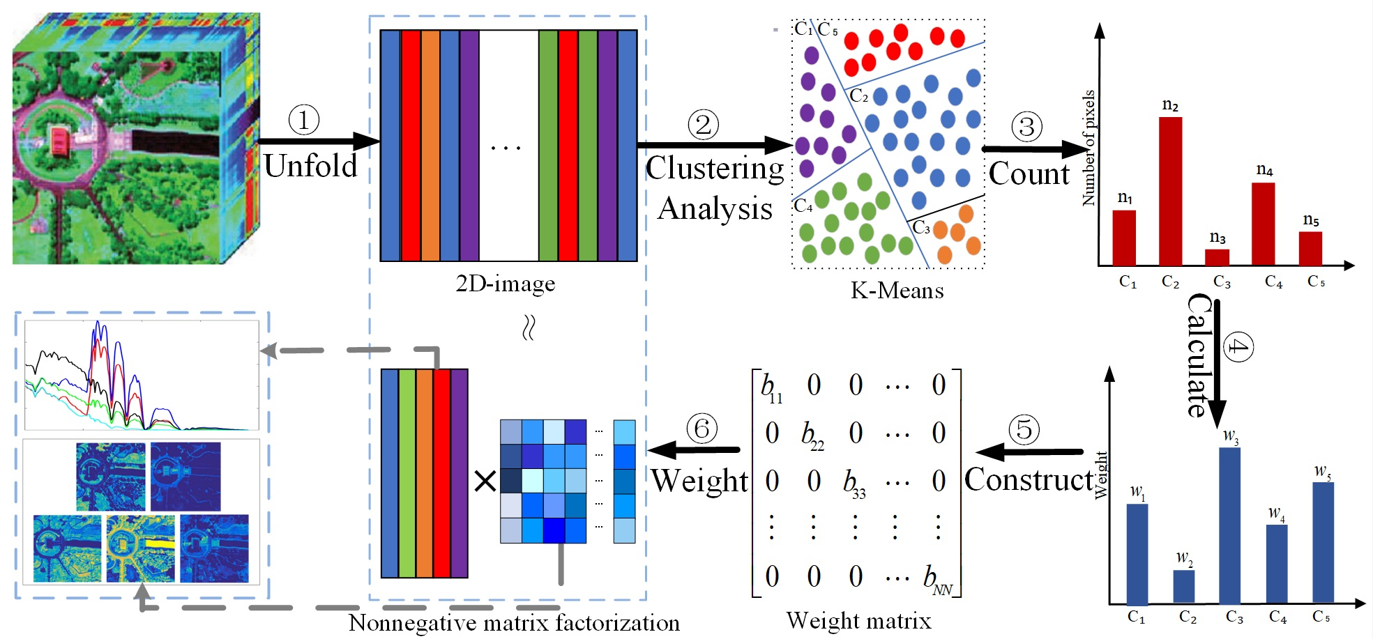
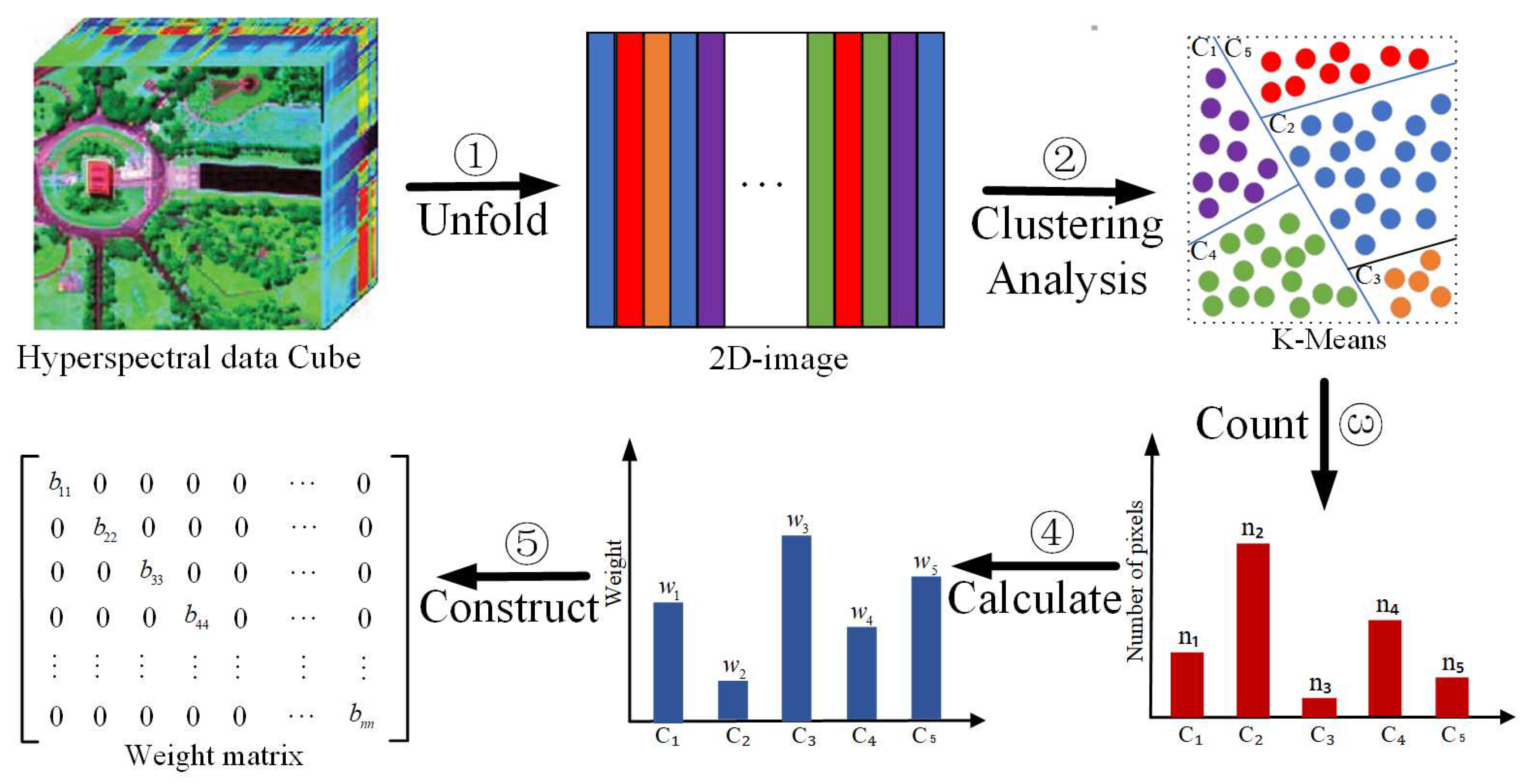
• We propose a novel NMF method for hyperspectral unmixing by exploiting the information of imbalance samples included in HSIs. Based on the clustering results of all the pixels, a weight matrix is generated to balance the impacts of each class of pixels to the reconstruction error of the standard NMF. This can reduce the adverse effect of imbalance samples to the estimation of endmembers that are only present in the pixels in a relatively small number, and thus improve the accuracy of the unmixing results.
• Our method provides a general framework for unmixing HSIs with imbalance pixels, and thus has good extensibility for incorporating additional constraints and regularization terms into the NMF-based unmixing model. Here, we extend the proposed method to other NMF-based unmixing approaches by adding the sparsity constraint of abundance and graph-based regularization, respectively.
• The performance of our methods is tested on both synthetic data and real-world HSIs. The experimental results show that our methods can achieve superior performance by comparing them with several state-of-the-art methods.

2. Related Work

In this paper, boldface uppercase letters are used to denote matrices, and the boldface lowercase letters are employed to represent vectors. Giving a matrix $\mathbf{Y}=[{\mathbf{y}}_1,{\mathbf{y}}_2,\dots ,{\mathbf{y}}_N]\in {\mathbb{R}}^{L\times N}$, we use ${\mathbf{Y}}_{ln}$ to represent the entry of $\mathbf{Y}$ in the l-th row and n-th column and ${\mathbf{Y}}^{\top }$ to indicate the transpose of the matrix. Using the symbol ${\mathbf{Y}}_{:n}$, we represent the n-th column vector of the matrix $\mathbf{Y}$. For $n\in \mathbb{N}$, $1_l$ is used to represent an all-one $n\times 1$ vector. Besides, ${\parallel ·\parallel }_F$ denotes the Frobenius norm of matrices, and the symbols “${}_{·}\ast$“ and “${}_{·}/$” represent the element-wise matrix multiplication and division, respectively.

Next, we will briefly introduce some basic concepts about LMM, NMF, and two representative variants of NMF.

2.1. Linear Mixing Model

Due to its simplicity and effectiveness, LMM has been adopted by many HU studies. In LMM, the observed spectrum of each pixel is regarded as a linear combination of a set of endmember signatures weighted by their abundance fractions. Mathematically, LMM can be expressed as

$$\mathbf{y}=\mathbf{A}\mathbf{s}+\mathbf{e},$$

(1)

where $\mathbf{y}\in {\mathbb{R}}^{L\times 1}$ is a vector denoting the observed pixel spectrum, $\mathbf{A}=[{\mathbf{a}}_1,{\mathbf{a}}_2,{\mathbf{a}}_3,\dots ,{\mathbf{a}}_P]\in {\mathbb{R}}^{L\times P}$ denotes the non-negative endmember matrix with each column representing an endmember signature, vector $\mathbf{s}\in {\mathbb{R}}^{P\times 1}$ stands for the abundance corresponding to $\mathbf{y}$, and $\mathbf{e}\in {\mathbb{R}}^{P\times 1}$ represents an additive noise vector. Besides, to make the model to be physically meaningful, all components of the abundance vector must satisfy with abundance non-negative constraint (ANC) and abundance sum-to-one constraint (ASC) [30], which are expressed as follows,

$$\mathrm{ANC}:s_j\ge 0,j=1,\dots ,P,$$

(2)

$$\mathrm{ASC}:\sum _{j=1}^P{s}_j=1.$$

(3)

From the point of matrix operation, LMM can be rewritten as a compact formulation, i.e.,

$$\mathbf{Y}=\mathbf{A}\mathbf{S}+\mathbf{E},$$

(4)

where $\mathbf{S}=[{\mathbf{s}}_1,{\mathbf{s}}_2,{\mathbf{s}}_3,\dots ,{\mathbf{s}}_N]\in {\mathbb{R}}^{P\times N}$ is the abundance matrix consisting of N abundance vectors, $\mathbf{E}\in {\mathbb{R}}^{L\times N}$ denotes the addition noise matrix, and L and P represent the number of band and endmember of the target HSI, respectively. Generally, only the observed hyperspectral data $\mathbf{Y}$ are known in the unmixing tasks, whereas the other two matrices $\mathbf{A}$ and $\mathbf{S}$ need to be estimated under constraint conditions ANC and ASC.

2.2. Non-Negative Matrix Factorization

As an effective blind source separation tool, NMF has attracted wide attention and received many successful applications in scientific and engineering fields. NMF aims to decompose a given non-negative matrix into two non-negative factor matrices with low ranks, so that the minimum error between the product of these factor matrices and the original matrix is minimized [31]. Formally, the standard NMF can be written as

$$\underset{\mathbf{A},\mathbf{S}}{min}{\parallel \mathbf{Y}-\mathbf{A}\mathbf{S}\parallel }_F^2,\mathrm{s}.\mathrm{t}.\mathbf{A},\mathbf{S}\ge 0,$$

(5)

where $\mathbf{Y}$ denotes the original matrix, $\mathbf{A}$ and $\mathbf{S}$ are two non-negative factor matrices, and the operator ${\parallel ·\parallel }_F$ denotes the Frobenius norm of matrices, whereas “≥” indicates the element-wise great than or equal to relationship between two matrices.

Because the objective function in Equation (5) is non-convex w.r.t the two factor matrices $\mathbf{A}$ and $\mathbf{S}$ simultaneously, the multiplication update rule (MUR) [19] based on the alternating optimization technique is commonly used to minimize $\mathbf{A}$ and $\mathbf{S}$. With MUR, each one of $\mathbf{A}$ and $\mathbf{S}$ is optimized with another being fixed in the algorithm iteration, and the corresponding update rules of them can be represented as follows,

$$\mathbf{A}\leftarrow {\mathbf{A}}_{·}\ast {\mathbf{Y}{\mathbf{S}}^{\top }}_{·}/\mathbf{A}\mathbf{S}{\mathbf{S}}^{\top },$$

(6)

$$\mathbf{S}\leftarrow {\mathbf{S}}_{·}\ast {\mathbf{A}}^{\top }{\mathbf{Y}}_{·}/{\mathbf{A}}^{\top }\mathbf{A}\mathbf{S}.$$

(7)

It is worth noting that the standard NMF suffers from the problems of being prone to trap into the local minimum and non-uniqueness of the solutions. One of the effective methods to tackle these problems is to introduce additional constraints or penalty terms into its objective function, so that the obtained solutions are more satisfied with the need for particular applications.

Considering the property of abundance sparseness of real HSIs, an unmixing method based on sparsity constrained NMF method, named $L_{1/2}$NMF, is proposed in [22], which adds the sparsity constraint of abundance into the standard NMF and leads to more satisfactory results than other sparse NMF methods. The objective function of $L_{1/2}$NMF is given by

$$f(\mathbf{A},\mathbf{S})=\frac{1}{2}{\parallel \mathbf{Y}-\mathbf{A}\mathbf{S}\parallel }_F^2+\lambda {\parallel \mathbf{S}\parallel }_{\frac{1}{2}},$$

(8)

where $\lambda$ is the regularization parameter used to weight the contribution of ${\parallel \mathbf{S}\parallel }_{\frac{1}{2}}$, which is expressed as follows,

$${\parallel \mathbf{S}\parallel }_{\frac{1}{2}}=\sum _{p=1}^P\sum _{n=1}^N{\left({\mathbf{S}}_{pn}\right)}^{\frac{1}{2}}.$$

(9)

However, $L_{1/2}$NMF often leads to quite different solutions giving different initial values. Moreover, the results obtained by $L_{1/2}$NMF are prone to noise interference. Therefore, it is necessary to exploit the structure of data to stabilize the sparse decomposition. Inspired by recent studies in manifold learning and sparse NMF, graph-regularized $L_{1/2}$NMF (GLNMF) [14] is proposed for HU. The objective function of GLNMF is expressed as follows,

$$f(\mathbf{A},\mathbf{S})=\frac{1}{2}{\parallel \mathbf{Y}-\mathbf{A}\mathbf{S}\parallel }_F^2+\lambda {\parallel \mathbf{S}\parallel }_{\frac{1}{2}}+\frac{\mu }{2}\mathrm{Tr}(\mathbf{S}Ł{\mathbf{S}}^{\top }),$$

(10)

where $\lambda$ and $\mu$ are regularization parameters; $\mathrm{Tr}(·)$ represents the trace of matrices; the regularization term $\mathrm{Tr}(\mathbf{S}Ł{\mathbf{S}}^{\top })$ plays the role of manifold constraint, in which $Ł=\mathbf{D}-\mathbf{W}$ is a Laplacian matrix; and $\mathbf{D}$ is a diagonal matrix with ${\mathbf{D}}_{ii}={\sum }_j{\mathbf{W}}_{ij}$, while $\mathbf{W}$ is the weight matrix of the graph constructed based on the HSI data. Given that ${\mathbf{y}}_j$ is one of the k-nearest neighbors of ${\mathbf{y}}_i$ according to the spectral distance, the weight matrix $\mathbf{W}$ of the graph is given via heat kernel as

$${\mathbf{W}}_{ij}=e^{-\frac{\parallel {\mathbf{y}}_i-{\mathbf{y}}_j{\parallel }^2}{\sigma }}.$$

(11)

As the GLNMF algorithm incorporates sparsity constraint and graph regularization simultaneously, it leads to a more desired unmixing performance. However, both $L_{1/2}$NMF and GLNMF neglect the imbalanced samples in real hyperspectral data, which restricts their performance.

3. Methodology

3.1. CW-NMF

In previous studies, most NMF-based unmixing methods have neglected the imbalanced samples included in many real hyperspectral images. In these data, there may be a large difference in the number of samples related to different endmembers, which is mainly caused by the imbalanced nature of the target distribution. For example, in a typical urban scenario, the dirt road only occupies a small number of areas compared with the asphalt road. As a result, endmembers with fewer samples are easy to be ignored due to the statistical characteristic of NMF, which causes the corresponding endmembers to be estimated with lower accuracy. Therefore, it is necessary to capture such imbalanced sample information to guide the NMF-based unmixing process. In this paper, we focus on the HU issue in the presence of imbalanced samples. To do so, we design a weighting mechanism that assigns appropriate weight value to each sample in the NMF-based unmixing procedure. With this strategy, the pixels that include imbalanced endmembers are assigned larger weight values, while the pixels mixed with majority endmembers are given smaller weight values. Consequently, the pixels with imbalanced endmembers have a significant impact on data reconstruction in the NMF-based model.

In our proposed unmixing model, we introduce a weight matrix into the objective function of the standard NMF, and the obtained objective function can be formally expressed as

$$f(\mathbf{A},\mathbf{S})=\frac{1}{2}{\parallel (\mathbf{Y}-\mathbf{A}\mathbf{S})\mathbf{B}\parallel }_F^2,$$

(12)

where $\mathbf{B}\in {\mathbb{R}}^{N\times N}$ is the diagonal weight matrix given by

$$\mathbf{B}=\left[\begin{array}{cccc}{b}_{11}& & & \\ & b_{22}& & \\ & & \ddots & \\ & & & b_{NN}\end{array}\right].$$

(13)

According to Equation (12), the diagonal element $b_{ii}$ of $\mathbf{B}$ plays the role of the weight of reconstruction error ${\mathbf{Y}}_{:i}-{\left(\mathbf{A}\mathbf{S}\right)}_{:i}$. In this way, we aim to enhance the impact of the pixel ${\mathbf{Y}}_{:i}$ in the data reconstruction if it contains imbalanced endmembers. On the contrary, if ${\mathbf{Y}}_{:i}$ is mixed with majority endmembers, the impact of ${\mathbf{Y}}_{:i}$ is reduced in the data reconstruction by a smaller value of $b_{ii}$. Based on this analysis, the proposed unmixing model is given as follows,

$$\underset{\mathbf{A},\mathbf{S}}{min}f(\mathbf{A},\mathbf{S})=\frac{1}{2}{\parallel (\mathbf{Y}-\mathbf{A}\mathbf{S})\mathbf{B}\parallel }_F^2,\mathrm{s}.\mathrm{t}.\mathbf{A},\mathbf{S}\ge 0.$$

(14)

It is worth noting that our proposed unmixing model has good extensibility for incorporating additional constraints and regularization terms, such as the sparsity constraint of abundance and graph-based regularization, which is demonstrated in Section 4.

Although the proposed CW-NMF model provides a general framework for unmixing HSIs with imbalanced samples, how to obtain the weight value related to each pixel remains a challenging work. To tackle this problem, as shown in Figure 1, we first conduct clustering analysis on the HSI matrix $\mathbf{Y}$ via K-means, so that different types of imbalanced samples are founded. Note that the number of clusters K is equal to the number of endmembers P for the sake of simplicity. Based on the clustering results $C=(C_1,C_2,\dots ,C_K)$, where $C_k,(k=1,2,\dots ,K)$ denotes a cluster, the number of pixels $n_k$ within each cluster $C_k$ is counted. Then, we compute the weight value $w_k$ associate with each cluster $C_k$ by

$$w_k=\frac{log\left(\frac{N}{n_k}\right)}{max(log\left(\frac{N}{\mathbf{v}}\right))},$$

(15)

where $\mathbf{v}=[n_1,n_2,\dots ,n_K]$ is a count vector, $max\left(\mathbf{x}\right)$ denotes a function used to obtain the maximum element in vector $\mathbf{x}$. In Equation (15), the numerator $log\left(\frac{N}{n_k}\right)$ is designed to give the basic weight information for each cluster $C_k$, which can not only provide distinct weight information for the clusters with different number pixels, but can also avoid a huge difference between them. As for the dominator $max(log\left(\frac{N}{\mathbf{v}}\right))$, we aim to restrict the weight value $w_k$ of each cluster in the interval [0, 1]. Note that all the pixels in the same cluster are assigned to the same weight value which equals to $w_k$ for the pixels in cluster $C_k$. For the convenience of representation, the symbol $b_{ii}$ that corresponds to the diagonal element of the matrix $\mathbf{B}$ is introduced to denote the weight values corresponding to pixel ${\mathbf{y}}_i$. In other words, if ${\mathbf{y}}_i\in C_k$, then $b_{ii}=w_k$. In this way, the pixels include imbalanced endmembers that have larger weight values and increase the impact of data reconstruction in the unmixing process.

3.2. Updating Rules

In the previous section, we have discussed the MUR of the standard NMF. Similar to the case of the standard NMF, the objective function described in Equation (12) is non-convex w.r.t factor matrices $\mathbf{A}$ and $\mathbf{S}$ simultaneously. Thus, it is hard to find the global minimum of them. Here, the alternating optimization technique is used to update $\mathbf{A}$ and $\mathbf{S}$. Specifically, let ${\mathsf{\Psi }}_{lp}⩾0$ and ${\mathsf{\Phi }}_{pn}⩾0$ be the corresponding Lagrange multipliers, the Lagrange function $\mathcal{L}$ corresponding to f in Equation (12) can be expressed as

$$\begin{array}{cc}\hfill \mathcal{L}& =\frac{1}{2}{\parallel (\mathbf{Y}-\mathbf{A}\mathbf{S})\mathbf{B}\parallel }_F^2+\mathrm{Tr}\left(\mathsf{\Psi }{\mathbf{A}}^{\top }\right)+\mathrm{Tr}\left(\mathsf{\Phi }{\mathbf{S}}^{\top }\right)\hfill \\ \hfill & =\frac{1}{2}\mathrm{Tr}\left(\mathbf{Y}\mathbf{B}{\mathbf{B}}^{\top }{\mathbf{Y}}^{\top }\right)+\mathrm{Tr}\left(\mathbf{Y}\mathbf{B}{\mathbf{B}}^{\top }{\mathbf{S}}^{\top }{\mathbf{A}}^{\top }\right)+\frac{1}{2}\mathrm{Tr}\left(\mathbf{A}\mathbf{S}\mathbf{B}{\mathbf{B}}^{\top }{\mathbf{S}}^{\top }{\mathbf{A}}^{\top }\right)+\mathrm{Tr}\left(\mathsf{\Psi }{\mathbf{A}}^{\top }\right)+\mathrm{Tr}\left(\mathsf{\Phi }{\mathbf{S}}^{\top }\right),\hfill \end{array}$$

(16)

where the definition of Frobenius norm ${\parallel \mathbf{A}\parallel }_F={\left(\mathrm{Tr}\left({\mathbf{A}}^{\top }\mathbf{A}\right)\right)}^{1/2}$ and two properties of trace $\mathrm{Tr}\left(\mathbf{A}\mathbf{S}\right)=\mathrm{Tr}\left(\mathbf{S}\mathbf{A}\right)$, $\mathrm{Tr}\left(\mathbf{A}\right)=\mathrm{Tr}\left({\mathbf{A}}^{\top }\right)$ are utilized to get the second equation. Then, by finding the partial derivative of $\mathbf{A}$ and $\mathbf{S}$, we can get

$$\begin{array}{cc}\hfill \frac{\partial \mathcal{L}}{\partial \mathbf{A}}& =-\mathbf{Y}\mathbf{B}{\mathbf{B}}^{\top }{\mathbf{S}}^{\top }+\mathbf{A}\mathbf{S}\mathbf{B}{\mathbf{B}}^{\top }{\mathbf{S}}^{\top }+\mathsf{\Psi },\\ \hfill \frac{\partial \mathcal{L}}{\partial \mathbf{S}}& =-{\mathbf{A}}^{\top }\mathbf{Y}\mathbf{B}{\mathbf{B}}^{\top }+{\mathbf{A}}^{\top }\mathbf{A}\mathbf{S}\mathbf{B}{\mathbf{B}}^{\top }+\mathsf{\Phi }.\end{array}$$

Resorting to the KKT conditions ${\mathsf{\Psi }}_{lp}{\mathbf{A}}_{lp}=0$ and ${\mathsf{\Phi }}_{pn}{\mathbf{S}}_{pn}=0$, it follows that

$$\begin{array}{cc}\hfill {(-\mathbf{Y}\mathbf{B}{\mathbf{B}}^{\top }{\mathbf{S}}^{\top }+\mathbf{A}\mathbf{S}\mathbf{B}{\mathbf{B}}^{\top }{\mathbf{S}}^{\top })}_{·}\ast \mathbf{A}& =0,\\ \hfill {(-{\mathbf{A}}^{\top }\mathbf{Y}\mathbf{B}{\mathbf{B}}^{\top }+{\mathbf{A}}^{\top }\mathbf{A}\mathbf{S}\mathbf{B}{\mathbf{B}}^{\top })}_{·}\ast \mathbf{S}& =0.\end{array}$$

Therefore, the updating rules for $\mathbf{A}$ and $\mathbf{S}$ can be obtained as

$$\mathbf{A}\leftarrow {\mathbf{A}}_{·}\ast \mathbf{Y}\mathbf{B}{\mathbf{B}}^{\top }{\mathbf{S}}_{·}^{\top }/\mathbf{A}\mathbf{S}\mathbf{B}{\mathbf{B}}^{\top }{\mathbf{S}}^{\top },$$

(17)

$$\mathbf{S}\leftarrow {\mathbf{S}}_{·}\ast {\mathbf{A}}^{\top }{\mathbf{Y}\mathbf{B}{\mathbf{B}}^{\top }}_{·}/{\mathbf{A}}^{\top }\mathbf{A}\mathbf{S}\mathbf{B}{\mathbf{B}}^{\top }.$$

(18)

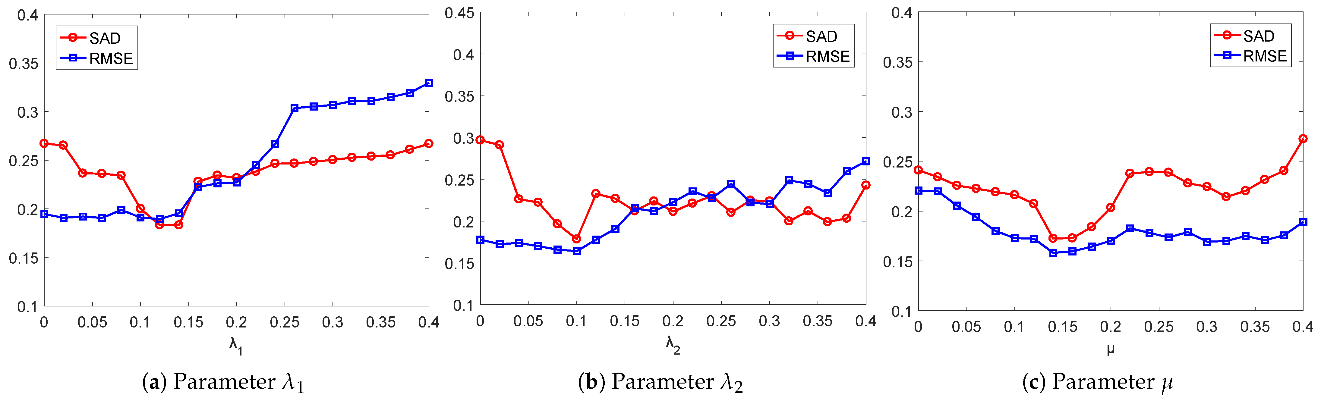
3.3. Implementation Issues

Here, several implementation issues for the proposed algorithm will be discussed in detail.

The first issue concerning the initialization strategies of the factor matrices $\mathbf{A}$ and $\mathbf{S}$. As the non-convex function Equation (14) is prone to obtain a local minimum, different initialization values of $\mathbf{A}$ and $\mathbf{S}$ will significantly affect the unmixing performance. In this paper, we adopt two initialization strategies: random initialization and VCA-FCLS initialization. To test the unmixing performance under general conditions, random initialization was employed in the experiments on synthetic data, where each entry of $\mathbf{A}$ and $\mathbf{S}$ was randomly set in the interval [0, 1]. The VCA-FCLS initialization was used in the experiments on real HSIs, by which the VCA algorithm provides effective initial values for $\mathbf{A}$, then the FCLS method initializes $\mathbf{S}$ based on the results given by VCA. In this way, the promising initial values are expected to be obtained, which is favorable for enhancing the unmixing performance.

The second issue is to guarantee the ANC and ASC in LMM. The updated formula indicated by Equations (17) and (18) can implicitly guarantee the ANC constraint when the initial values of $\mathbf{A}$ and $\mathbf{S}$ are non-negative. To ensure the ASC constraint, following the measure in [22], we augment matrices $\mathbf{Y}$ and $\mathbf{A}$ by appending a row with all-one vector, respectively. Based on this strategy, the matrices $\mathbf{Y}$ and $\mathbf{A}$ in Equation (18) will be substituted by $\overline{\mathbf{Y}}$ and $\overline{\mathbf{A}}$, which is given by

$$\overline{\mathbf{Y}}=\left[\begin{array}{c}\mathbf{Y}\\ \delta 1_N^{\top }\end{array}\right],\overline{\mathbf{A}}=\left[\begin{array}{c}\mathbf{A}\\ \delta 1_P^{\top }\end{array}\right],$$

(19)

where $\delta$ is a parameter to adjust the impact of ASC. Note that the higher $\delta$ can lead to a more satisfied ASC constraint but will cause a slower convergence rate [14]. To balance these two factors, we set the parameter $\delta =20$ in our experiment.

Another issue is stopping criteria. In general, the most commonly used method is to set the error tolerance or maximum iteration number. In our work, if the error tolerance of objective function $f(\mathbf{A},\mathbf{S})$ in successive iteration does not exceed the predefined threshold value for ten times, our algorithm will terminate. At the same time, the iteration number of our algorithms is limited by the predefined maximum iteration number. In the experiments, we set the maximum iteration number to 3000.

The last one is how to determine the number of endmembers. Recently, two effective methods, i.e., virtual dimensionality [32] and hyperspectral signal identification by minimum error (HySime) [33] are frequently used to estimate the number of endmembers. However, we assumed the number of endmembers is known a priori in our experiments [14,21,22].

Based on the above method, the proposed CW-NMF algorithm is given in Algorithm 1.

Algorithm 1 CW-NMF Algorithm For HU

3.4. Computational Complexity Analysis

Here, the computational complexity of the proposed CW-NMF method will be discussed. For ease of calculation, the time of floating-point calculation is counted for each iteration to analyze the computational complexity. As shown in Algorithm 1, the main computation cost involves updates $\mathbf{A}$ and $\mathbf{S}$ in Equations (17) and (18), respectively. By referring to Equations (17) and (18) corresponding to MURs of CW-NMF, as well as Equations (6) and (7) representing MURs of standard NMF, we can see that the only difference between the CW-NMF and standard NMF method is the existence of the weight matrix $\mathbf{B}$. Consequently, we analyze the computation cost of the CW-NMF based on the standard NMF results. First, the computational complexity of the standard NMF is $O\left(LNP\right)$ [14]. As for the update of $\mathbf{A}$, it is noted that the order of the matrix multiplication is important [34], such as $\left(\mathbf{Y}\mathbf{B}\right){\mathbf{B}}^{\top }$ and $\mathbf{Y}\left(\mathbf{B}{\mathbf{B}}^{\top }\right)$, leads to different computational costs under different order. The former needs $O\left(2L{N}^2\right)$, whereas the latter costs $O(N^3+N^{2}L)$ times. As $L\ll N$, the $O\left(2L{N}^2\right)\ll O(N^3+N^{2}L)$, which means that $\mathbf{Y}\left(\mathbf{B}{\mathbf{B}}^{\top }\right)$ is much more complex than $\left(\mathbf{Y}\mathbf{B}\right){\mathbf{B}}^{\top }$. Besides, the weight matrix $\mathbf{B}$ given in the proposed CW-NMF algorithm is a diagonal matrix, i.e., there is only one nonzero element in each row of the matrix $\mathbf{B}$. The $\left(\mathbf{Y}\mathbf{B}\right){\mathbf{B}}^{\top }$ costs about $O\left(L{N}^2\right)$ times under this condition. Therefore, the process of the update $\mathbf{A}$ costs $O\left(L{N}^2\right)$ for one iteration. Similarly, the cost of computing $\mathbf{S}$ is $O\left(L{N}^2\right)$. Taking all factors into consideration, the total cost of CW-NMF is $O\left(mL{N}^2\right)$ when the iteration stops after m steps.

4. Method Extension

The proposed CW-NMF method provides a general framework for making use of the information on imbalanced data in real HSIs. Thus, it is natural to consider extending it to other NMF-based unmixing methods, such as $L_{1/2}$NMF and GLNMF methods, which will be discussed in this section.

4.1. CW-$L_{1/2}$NMF

As aforementioned, the $L_{1/2}$NMF algorithm improves the unmixing performance by incorporating the sparsity constraint of abundance into the unmixing model. However, $L_{1/2}$NMF only considers the sparseness of the data, which leads to unstable decomposition results and poor noise robustness. To tackle this issue, we introduced the proposed weight matrix into $L_{1/2}$NMF, so that we can simultaneously exploit the information of imbalanced samples and the sparsity property of abundances. Specifically, the weight matrix $\mathbf{B}$ is extended to $L_{1/2}$NMF (named CW-$L_{1/2}$NMF), and the obtained objective function can be expressed as

$$f(\mathbf{A},\mathbf{S})=\frac{1}{2}{\parallel (\mathbf{Y}-\mathbf{A}\mathbf{S})\mathbf{B}\parallel }_F^2+{\lambda }_1{\parallel \mathbf{S}\parallel }_{\frac{1}{2}},$$

(20)

where $\mathbf{B}$ is the weight matrix calculated by Equation (15). It is easy to see that MUR of $\mathbf{A}$ in Equation (20) is the same as Equation (17). According to the deduction of MUR about $\mathbf{S}$ in [22] and Equation (18), MUR of $\mathbf{S}$ in Equation (20) are obtained and presented as

$$\mathbf{S}\leftarrow {\mathbf{S}}_{·}\ast {\mathbf{A}}^{\top }{\mathbf{Y}\mathbf{B}{\mathbf{B}}^{\top }}_{·}/({\mathbf{A}}^{\top }\mathbf{A}\mathbf{S}\mathbf{B}{\mathbf{B}}^{\top }+\frac{1}{2}{\lambda }_1{\mathbf{S}}^{-\frac{1}{2}}).$$

(21)

4.2. CW-GLNMF

As has been mentioned in Section 2.2, GLNMF aims to improve the performance of $L_{1/2}$NMF by assuming that the samples are distributed on a low-dimensional manifold in a high-dimensional Euclidean space and exploiting the manifold structure of data via the graph-based regularization. To effectively utilize the prior information of imbalanced samples in the data during the unmixing procedure of GLNMF, we have introduced the weight matrix into the objective function of GLNMF, and the obtained cluster-wise weighted GLNMF (named CW-GLNMF) unmixing model is given as

$$f(\mathbf{A},\mathbf{S})=\frac{1}{2}{\parallel (\mathbf{Y}-\mathbf{A}\mathbf{S})\mathbf{B}\parallel }_F^2+{\lambda }_2{\parallel \mathbf{S}\parallel }_{\frac{1}{2}}+\frac{\mu }{2}\mathrm{Tr}(\mathbf{S}Ł{\mathbf{S}}^{\top }),$$

(22)

where ${\lambda }_2$ and $\mu$ are regularization parameters used to adjust the impact of sparsity constraint imposed on $\mathbf{S}$ and the graph-based regularization, respectively; $\mathbf{B}$ is the introduced weight matrix that is constructed according to Equation (15). By referring to the deduction procedure of Equation (18) and MUR of $\mathbf{S}$ in GLNMF [14], we can get MUR of $\mathbf{S}$ in CW-GLNMF as

$$\begin{array}{c}\hfill \mathbf{S}\leftarrow {\mathbf{S}}_{·}\ast {({\mathbf{A}}^{\top }\mathbf{Y}\mathbf{B}{\mathbf{B}}^{\top }+\mu \mathbf{S}\mathbf{W})}_{·}/({\mathbf{A}}^{\top }\mathbf{A}\mathbf{S}\mathbf{B}{\mathbf{B}}^{\top }+\frac{1}{2}{\lambda }_2{\mathbf{S}}^{-\frac{1}{2}}+\mu \mathbf{S}\mathbf{D}),\end{array}$$

(23)

whereas MUR of $\mathbf{A}$ remains the same as the CW-NMF solution, i.e., it is identical to Equation (17).

5. Experimental Results

In this section, a series of experiments on synthetic and real hyperspectral data sets are conducted to evaluate the performance of the proposed methods: CW-NMF, CW-$L_{1/2}$NMF, and CW-GLNMF. For the experiments on synthetic data sets, our methods are compared with NMF, $L_{1/2}$NMF, and GLNMF. When our methods are tested on real hyperspectral data, they are compared with four representative algorithms, i.e., NMF, $L_{1/2}$NMF, GLNMF, SGSNMF, and VCA followed by FCLS (VCA-FCLS), in which the first four are NMF-based unmixing methods, whereas VCA is a famous geometry-based method for endmember extraction. As VCA can only extract endmember from data, we estimate the corresponding abundances by the FCLS method based on the results given by VCA. Note that all the algorithms are tested 20 times and the average performance is reported. In the experiment, spectral angle distance (SAD) and root mean square error (RMSE), which have been widely adopted in the existing works, are used to measure the accuracy of estimated endmembers, as well as their corresponding abundances, respectively. Specifically, for the p-th endmember, the SAD between the reference signature ${\mathbf{A}}_p$ and the estimated one ${\hat{\mathbf{A}}}_p$ is defined as

$${\mathrm{SAD}}_p=arccos\left(\frac{{\hat{\mathbf{A}}}_p{}^{\top }{\mathbf{A}}_p}{\parallel {\hat{\mathbf{A}}}_p\parallel \parallel {\mathbf{A}}_p\parallel }\right),$$

(24)

where $\parallel ·\parallel$ represents the Euclidean norm of vectors. To evaluate the difference between the reference abundances ${\mathbf{S}}_p$ corresponding to the p-th endmember and the estimated abundances ${\hat{\mathbf{S}}}_p$, the RMSE criterion is adopted and defined as

$${\mathrm{RMSE}}_p={\left(\frac{1}{N}|{\hat{\mathbf{S}}}_p-{\mathbf{S}}_p{|}^2\right)}^{\frac{1}{2}}.$$

(25)

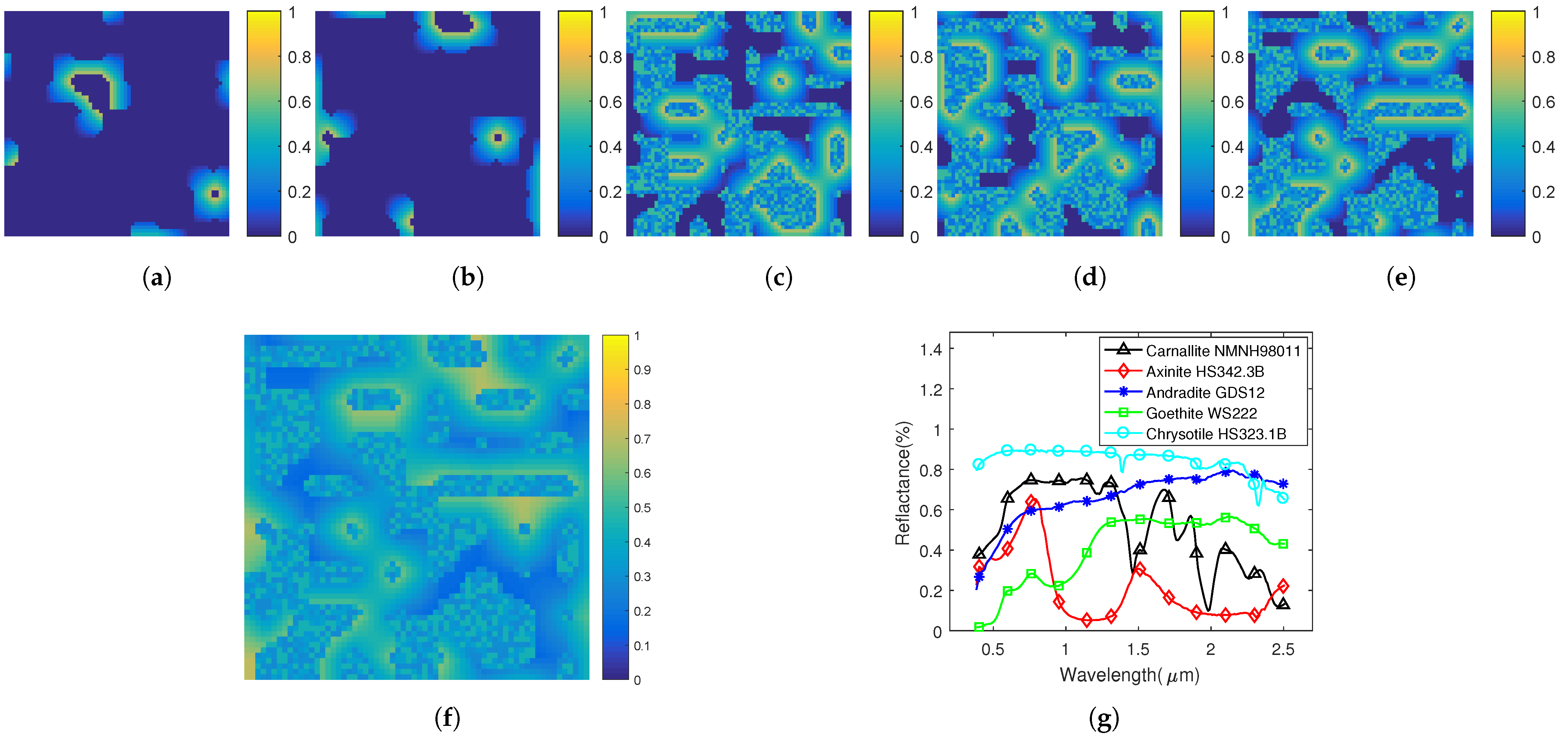
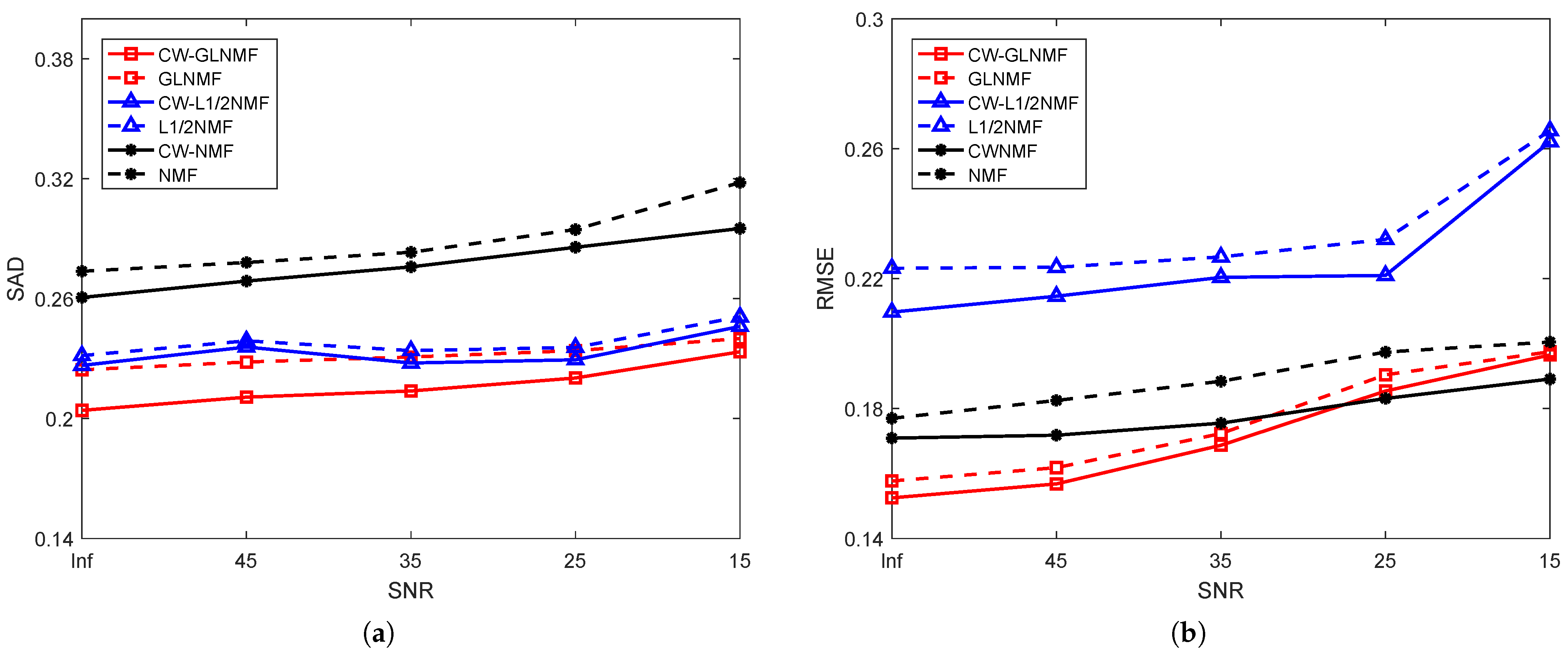
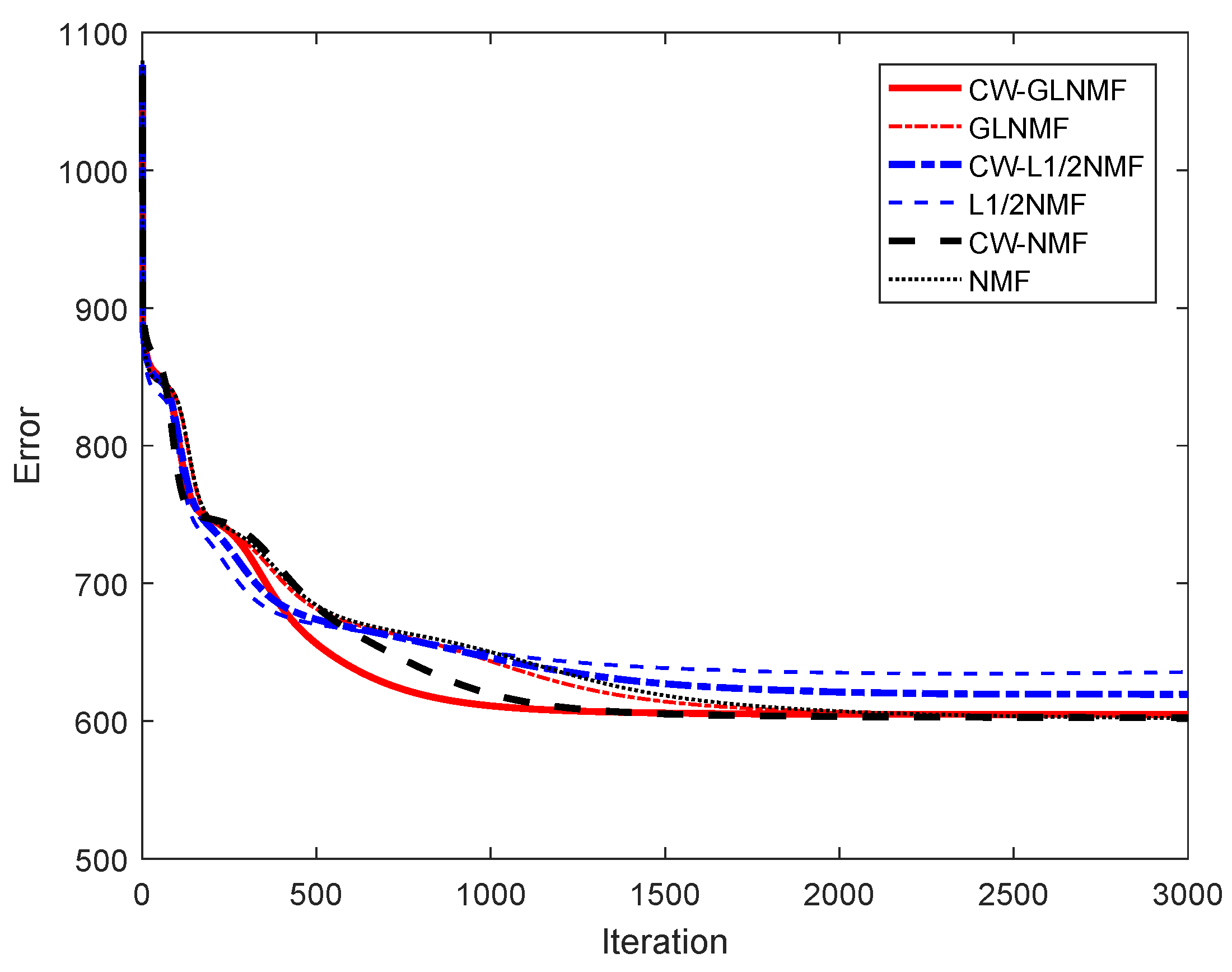
5.1. Experiments on Synthetic Data

To generate the synthetic data set, five real spectral signatures are randomly chosen from the United States Geological Survey (USGS) digital spectral library. These selected signatures contain 224 spectral bands with wavelengths from 0.38 to 2.5 $\mathsf{\mu }$m. Based on them, the synthetic data sets are generated by the modified process in [22]: (1) an image of size 64 × 64 pixels is divided into 8 × 8 blocks and all blocks are of the same size; (2) ten blocks among 64 blocks are randomly selected. Then, five blocks of the chosen blocks are covered by the same type of designated endmembers, and the rest five blocks are also filled with a kind of specified endmember. The remaining blocks are filled by the randomly selected endmembers from another three types of endmembers so that each block is covered with only one type of material; (3) a 9 × 9 low-pass filter is applied to the image to get mixed pixels, and the abundance vector corresponding to each pixel is obtained; (4) to adjust the mixing degree of the synthetic data, the pixel whose abundance is larger than a preset parameter $\theta$ will be replaced with a mixture of three randomly selected endmembers with equal ratio; and (5) to test the robustness of our methods to noise interference, we add zero-mean white Gaussian noise of different signal-to-noise ration (SNR) to the obtained synthetic data set. Here, SNR is defined as

$$\mathrm{SNR}=10{log}_{10}\frac{E\left[{\mathbf{y}}^{\top }\mathbf{y}\right]}{E\left[{\mathbf{e}}^{\top }\mathbf{e}\right]},$$

(26)

where $\mathbf{y}$ and $\mathbf{e}$ represent the observation vector and noise vector of a pixel, respectively; $E[·]$ denotes the expectation operator. As an example of the synthetic data, Figure 2a–f shows the abundance maps and the 188th band of a 64 × 64 synthetic data with SNR of 25 dB, respectively, and Figure 2g gives the curves of the selected endmembers.

Experiment 1 (select the algorithm parameters): In this section, several experiments are designed to determine the optimal values of parameters ${\lambda }_1$, ${\lambda }_2$, and $\mu$ with the synthetic data generated under the condition that $\mathrm{SNR}=25$ dB, $P=5$, and $\theta =0.7$. Note that parameter ${\lambda }_1$ is the regularization parameter of the method CW-$L_{1/2}$NMF, while ${\lambda }_2$ and $\mu$ are the regularization parameters of CW-GLNMF. To decrease the influence of random initialization, the same initial $\mathbf{A}$ and $\mathbf{S}$ are used in both CW-$L_{1/2}$NMF and CW-GLNMF throughout the experiments. First, the parameter ${\lambda }_1$ in the extended algorithm CW-$L_{1/2}$NMF is tested. Figure 3a shows the performance of CW-$L_{1/2}$NMF when the value ${\lambda }_1$ is changed from 0 to 0.4 with an interval of 0.02. As shown in Figure 3a, the SAD decreased in the interval [0, 0.12], whereas increased in the interval [0.14, 0.4]. The CW-$L_{1/2}$NMF shows better performance when parameter ${\lambda }_1$ varies from 0.12 to 0.14. As for the RMSE values, they are stable in the interval [0, 0.16] and increase in the interval [0.16, 0.4], indicating the worse performance of CW-$L_{1/2}$NMF. On the whole, CW-$L_{1/2}$NMF obtained better performance in the interval [0.12, 0.14], and we set ${\lambda }_1=0.12$ in the experiments.

Next, we select the optimal value of the parameter $\mu$ of the proposed CW-GLNMF method when ${\lambda }_2$ is set to 0.1. We test the performance of CW-GLNMF by altering the value $\mu$ from 0 to 0.4 with a step size of 0.02. The obtained SAD and RMSE results are given in Figure 3c. As can be seen from Figure 3c, the values of the SAD decreased when $\mu$ varies in the interval [0, 0.14], and it increased with $\mu$ changing from 0.16 to 0.22. It is easy to see that better SAD performances of CW-GLNMF can be achieved in the interval [0.14, 0.18]. Besides, the RMSE values decrease in the case of $\mu$ in the interval [0, 0.14], and it remains stable and better values under the condition that $\mu$ changes from 0.14 to 0.4. Overall, CW-GLNMF can provide better SAD and RMSE performance when $\mu$ varies from 0.14 to 0.16. Thus, the average value of $\mu =0.15$ can be selected as a better parameter.

Here, we test another parameter, ${\lambda }_2$, of the CW-GLNMF algorithm by fixing $\mu =0.15$. Similarly, the value of ${\lambda }_2$ is set to change between 0 and 0.4 with an interval of 0.02. Figure 3b shows the unmixing performance of CW-GLNMF w.r.t. SAD and RMSE criteria. From Figure 3b, we can see the SAD value is decrease when ${\lambda }_2$ locates in the interval [0, 0.1], and the least value is obtained in the case of ${\lambda }_2=0.1$. Concerning the RMSE criterion, it has stable and small values when ${\lambda }_2$ varies from 0 to 0.1, whereas its values get larger in the interval [0.1, 0.4]. In general, our CW-GLNMF method provides its minima when parameter ${\lambda }_2=0.1$. To sum up, the following experiments are implemented based on ${\lambda }_1=0.12$, ${\lambda }_2=0.1$ and $\mu =0.15$.

Experiment 2 (robustness of the algorithm under different noises): This experiment is designed to test the robustness of the six NMF-based algorithms on synthetic data with different noises. In our experiment, we only change the value of SNR from infinity (noise-free) to 15 dB with an interval of 10 dB. Figure 4 provides the average performance of six algorithms when they are tested on the data with different SNR. From Figure 4, we can see that the performance of these methods become worse when the value of SNR decreases. According to SAD values, Figure 4a shows that the CW-NMF has an obvious advantage by providing smaller values than the NMF method when SNR varies. CW-$L_{1/2}$NMF also gives slightly better SAD values when compared with $L_{1/2}$NMF. Meanwhile, CW-GLNMF obtains the smallest SAD values than GLNMF, indicating that CW-GLNMF can achieve more accurate endmembers. As for the RMSE values shown in Figure 4b, CW-NMF is superior to NMF as it has been given a smaller RMSE value, and CW-$L_{1/2}$NMF has better performance than $L_{1/2}$NMF on the data with different SNR. It is easy to see that the CW-GLNMF not only has smaller RMSE values than GLNMF, but also provides the best RMSE values on the data with SNR changing from infinity to 35 dB. Generally, our proposed algorithms outperform the other three representative methods at alterative, respectively, which verifies the robustness to the noise of our proposed algorithms.

Experiment 3 (convergence analysis): In this experiment, we analyze the convergence of our proposed methods and the other three methods. We test all six methods on the synthetic data that are generated under the condition that $\mathrm{SNR}=25$ dB, $P=5$, and $\theta =0.7$. The approximation errors between the original and reconstruction data by product of the matrix given by all the methods are plotted in Figure 5. As shown in Figure 5, the plots of appropriation error decrease as the iteration number varies from 0 to 2000, and then keep stable when the iteration number in the interval [2000, 3000], indicating those curves are convergence. Moreover, CW-NMF has a similar reconstruct error, but achieves a better convergence rate at the early stages of the optimization process. As for CW-$L_{1/2}$NMF and $L_{1/2}$NMF, we can see that CW-$L_{1/2}$NMF has a better reconstruct error. By comparing with the GLNMF algorithm, CW-GLNMF shows obvious superiority in the convergence rate. Consequently, our methods can reach faster convergence within 3000 times, and obtain similar error with another three methods.

Experiment 4 (factor exploration): Here, some visual results are shown to provide an intuitive evaluation of the effectiveness of our proposed weight matrix $\mathbf{B}$. By conducting clustering analysis via the K-means method on the synthetic data with five endmembers, we obtained the matrix $\mathbf{B}$ according to Algorithm 1, whose diagonal elements are composed of $w_k,(k=1,2,3,4,5)$. Figure 6 gives five visual images of the weight matrix $\mathbf{B}$, where each image is represented by a manner of the heat map, and non-zero pixels in the k-th image has the value of $w_k$. Note that the pixel with high color temperature indicates a large weight of the corresponding pixel. By comparing Figure 2a–e with Figure 6a–e, respectively, the weight matrix $\mathbf{B}$ has a good similarity to the reference abundances of synthetic data. Thus, it reveals that the introduction of weight matrix $\mathbf{B}$ is reasonable and effective both on theoretical analysis and experimental verification.

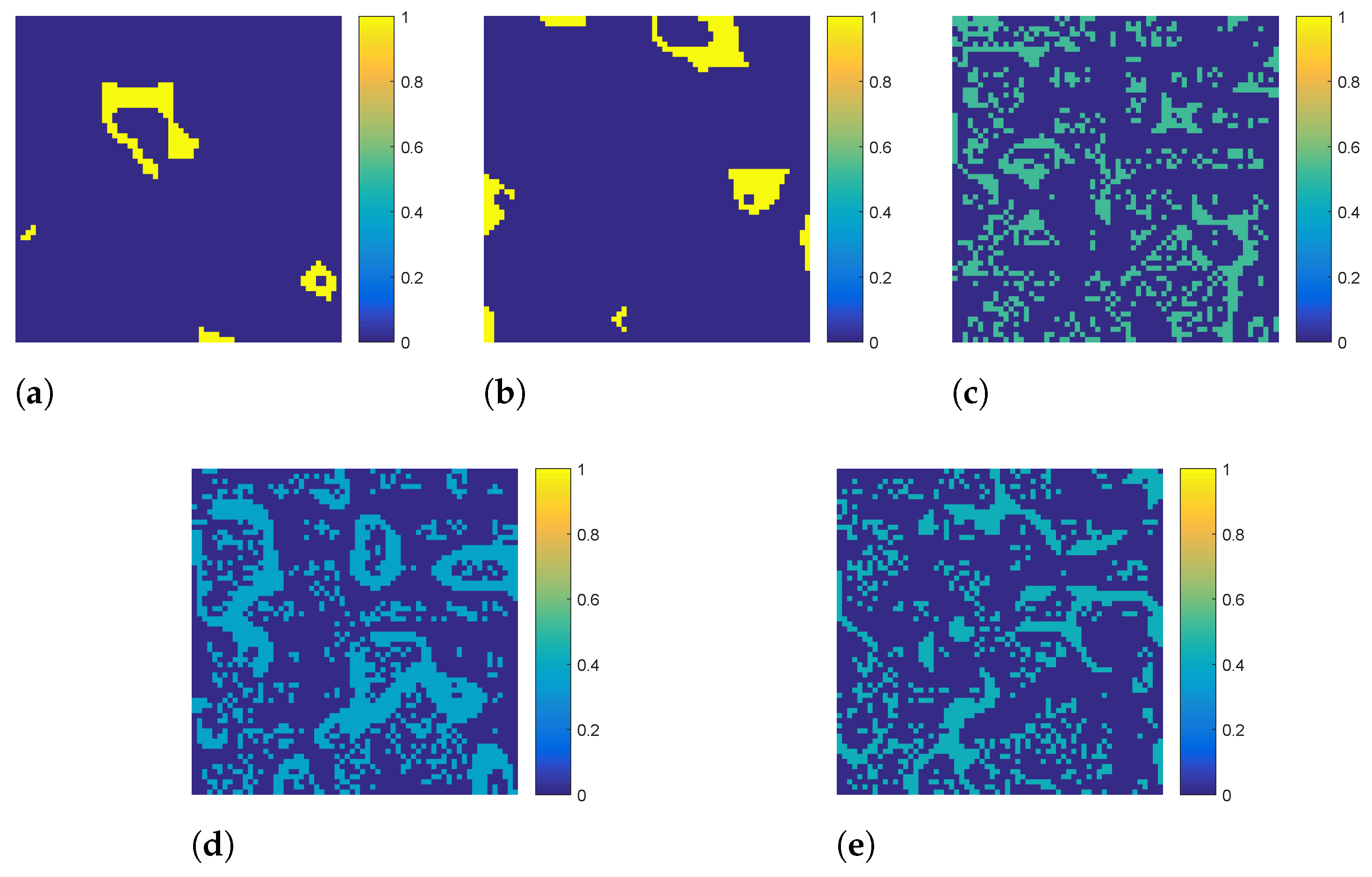
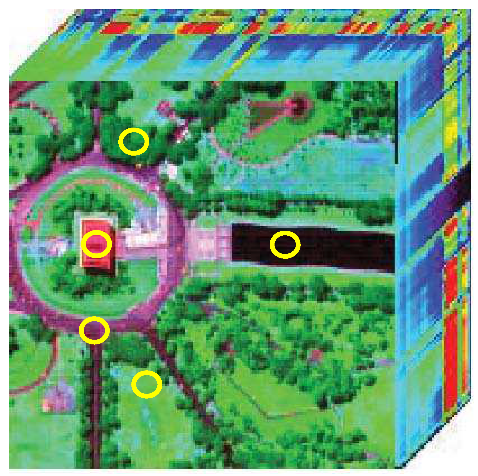
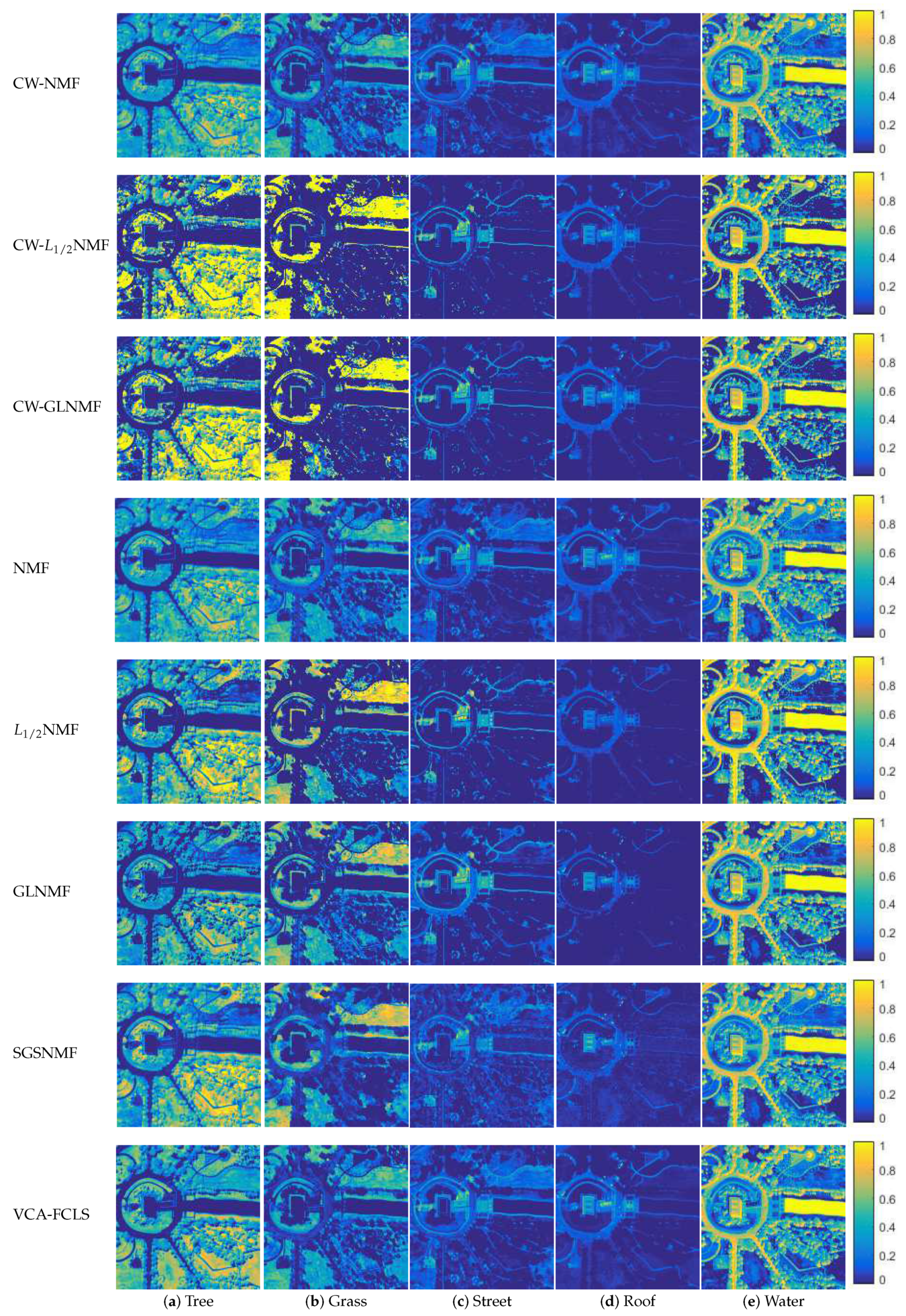
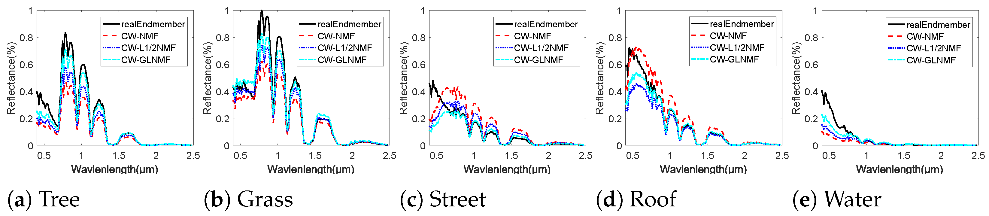
5.2. Experiments on Real Hyperspectral Data

To validate the performance of the proposed methods, we conduct several experiments on the real-world hyperspectral data. Here, the Washington DC Mall hyperspectral data acquired by the Hyperspectral Digital Imagery Collection Experiment (HYDICE) sensor is applied to compare the proposed methods with VCA-FCLS, NMF, $L_{1/2}$NMF, GLNMF, and SGSNMF [21].

The original Washington DC Mall hyperspectral data consists of 210 spectral bands with wavelengths from 0.4 to 2.5 $\mathsf{\mu }$m. In our experiments, a sub-image with a size of 150 × 150 pixels is extracted from the original image, which contains five ground-truth materials of interest: Tree, Grass, Street, Roof, and Water. Before unmixing, we removed the low SNR and water vapor absorption bands (including bands 103–106, 138–148, and 207–210) from the data, leaving 191 bands. Note that each type of reference endmember of the HYDICE Washington DC Mall data is generated by first manually choosing 15 pixels from the original data cube, then computing the average value of the selected pixels. Figure 7 shows the 3D cube of Washington DC Mall data, in which the yellow circles indicate the position where the pixels used to generate the reference endmembers are chosen. According to the distribution proportion of the interesting materials in the scene shown in Figure 7, we assume that the street corresponds to the imbalanced endmember.

To test the accuracy of the endmember extraction of our methods quantitatively,

Table 1. Performance comparison on the HYDICE Washington DC Mall data, where the red bold and blue italic fonts denote the best and second-best results, respectively. In addition, the black bold letters represent the imbalanced endmember.

Endmembers	CW-NMF	CW-${\mathit{L}}_{1/2}$NMF	CW-GLNMF	NMF [19]	${\mathit{L}}_{1/2}$NMF [22]	GLNMF [14]	SGSNMF [21]	VCA [12]
Tree	0.2177 ± 2.66	0.1732 ± 12.48	0.1462 ± 16.26	0.2413 ± 8.01	0.1842 ± 1.18	0.1821 ± 14.30	0.1763 ± 1.03	0.2018 ± 0.67
Grass	0.2906 ± 5.61	0.1296 ± 8.98	0.1557 ± 10.44	0.2559 ± 4.68	0.2345 ± 4.11	0.2102 ± 6.67	0.1646 ± 19.78	0.2699 ± 6.56
Roof	0.1261 ± 3.82	0.1785 ± 3.21	0.1482 ± 2.48	0.1428 ± 3.57	0.1670 ± 4.43	0.1600 ± 3.61	0.3019 ± 6.79	0.1505 ± 4.10
Water	0.1738 ± 25.42	0.2437 ± 20.25	0.1857 ± 33.39	0.1936 ± 27.86	0.1734 ± 15.60	0.1402 ± 11.68	0.1226 ± 1.16	0.2144 ± 28.12
Street	0.4342 ± 18.87	0.4295 ± 13.67	0.4227 ± 16.52	0.4642 ± 14.46	0.4456 ± 12.57	0.4716 ± 15.56	0.4905 ± 28.98	0.4827 ± 11.57
Average	0.2485 ± 11.27	0.2309 ± 11.72	0.2117 ± 15.82	0.2596 ± 11.72	0.2409 ± 7.58	0.2328 ± 10.36	0.2512 ± 11.55	0.2639 ± 10.20

lists the SAD values corresponding to different endmembers, the standard deviations of the SAD values, as well as their average values given by all of the methods. As shown in Table 1, the proposed CW-NMF method has better performance than the NMF method by providing three better cases and decreasing the average SAD value of $4.3\%$ compared with the NMF method. As for the imbalanced endmember, CW-NMF decreases the SAD value of $6.4\%$ than the NMF method. By comparing the SAD values given by $L_{1/2}$NMF and CW-$L_{1/2}$NMF, our proposed CW-$L_{1/2}$NMF method outperforms the $L_{1/2}$NMF by providing lower average SAD value and more best cases. Besides, CW-$L_{1/2}$NMF method provides the second-best SAD value about the imbalanced endmember and it reduces the SAD value of $3.6\%$ compared with $L_{1/2}$NMF. In addition, the proposed CW-GLNMF method shows the best performance by giving two best cases and best average SAD value. Compared with GLNMF, CW-GLNMF decreases the SAD value of $10.3\%$ about the imbalanced endmember. To provide visual comparisons, Figure 8 shows color images of the estimated abundance maps given by all the methods, where brighter pixels represent a higher abundance of the relative endmember in the map. In addition, we plot the endmember signatures obtained by CW-NMF, CW-$L_{1/2}$NMF, and CW-GLNMF algorithms, as well as the reference endmember in Figure 9. We can see from Figure 9 that the estimated endmembers have good similarity with the corresponding reference signatures, and the CW-GLNMF algorithm shows the best consistency than the other two methods.

6. Conclusions

In this paper, we have proposed a cluster-wise weighted NMF method for hyperspectral unmixing by exploiting the information of imbalanced samples in hyperspectral images. Specifically, a weight matrix constructed based on the results of clustering analysis on the data is incorporated into the standard NMF model, which effectively reduces the influence of imbalanced samples in the data to the statistical performance of NMF, so that the unmixing results can give more accurate endmembers and abundances. Moreover, the proposed NMF-based unmixing method provides a general framework for unmixing hyperspectral data with imbalanced samples, which is demonstrated by extending the proposed method by adding the sparsity constraints of abundance or graph-based regularization. A series of experiments on both synthetic and real hyperspectral data has demonstrated that the proposed methods outperformed several state-of-the-art methods.

References

1. Zhang, W.; Lu, X.; Li, X. Similarity Constrained Convex Nonnegative Matrix Factorization for Hyperspectral Anomaly Detection. IEEE Trans. Geosci. Remote Sens. 2019, 57, 4810–4822. [Google Scholar] [CrossRef]
2. Jiang, J.; Ma, J.; Wang, Z.; Chen, C.; Liu, X. Hyperspectral Image Classification in the Presence of Noisy Labels. IEEE Trans. Geosci. Remote Sens. 2019, 57, 851–865. [Google Scholar] [CrossRef] [Green Version]
3. Ma, L.; Crawford, M.M.; Zhu, L.; Liu, Y. Centroid and Covariance Alignment-Based Domain Adaptation for Unsupervised Classification of Remote Sensing Images. IEEE Trans. Geosci. Remote Sens. 2019, 57, 2305–2323. [Google Scholar] [CrossRef]
4. Nalepa, J.; Myller, M.; Kawulok, M. Validating Hyperspectral Image Segmentation. IEEE Geosci. Remote Sens. Lett. 2019, 16, 1264–1268. [Google Scholar] [CrossRef] [Green Version]
5. Swarna, M.; Sowmya, V.; Soman, K.P. Band selection using variational mode decomposition applied in sparsity-based hyperspectral unmixing algorithms. Signal Image Video Process. 2018, 12, 1463–1470. [Google Scholar] [CrossRef]
6. Bioucas-Dias, J.M.; Plaza, A.; Dobigeon, N.; Parente, M.; Du, Q.; Gader, P.; Chanussot, J. Hyperspectral Unmixing Overview: Geometrical, Statistical, and Sparse Regression-Based Approaches. IEEE J. Sel. Top. Appl. Earth Observ. Remote Sens. 2012, 5, 354–379. [Google Scholar] [CrossRef] [Green Version]
7. Wang, W.; Qian, Y.; Liu, H. Multiple Clustering Guided Nonnegative Matrix Factorization for Hyperspectral Unmixing. IEEE J. Sel. Top. Appl. Earth Observ. Remote Sens. 2020, 13, 5162–5179. [Google Scholar] [CrossRef]
8. Dobigeon, N.; Tourneret, J.; Richard, C.; Bermudez, J.C.M.; McLaughlin, S.; Hero, A.O. Nonlinear Unmixing of Hyperspectral Images: Models and Algorithms. IEEE Signal Process. Mag. 2014, 31, 82–94. [Google Scholar] [CrossRef] [Green Version]
9. Ma, W.; Bioucas-Dias, J.M.; Chan, T.; Gillis, N.; Gader, P.; Plaza, A.J.; Ambikapathi, A.; Chi, C. A Signal Processing Perspective on Hyperspectral Unmixing: Insights from Remote Sensing. IEEE Signal Process. Mag. 2014, 31, 67–81. [Google Scholar] [CrossRef] [Green Version]
10. Boardman, J.W. Automated spectral unmixing of AVIRIS data using convex geometry concepts. In Proceedings of the JPL Airborne Geoscience Workshop, Arlington, VA, USA, 25–29 October 1993; Volume 1, pp. 11–14. [Google Scholar]
11. Winter, M.E. N-FINDR: An algorithm for fast autonomous spectral end-member determination in hyperspectral data. Proc. SPIE Int. Soc. Opt. Eng. 1999, 3753, 266–275. [Google Scholar]
12. Nascimento, J.M.P.; Dias, J.M.B. Vertex component analysis: A fast algorithm to unmix hyperspectral data. IEEE Trans. Geosci. Remote Sens. 2005, 43, 898–910. [Google Scholar] [CrossRef] [Green Version]
13. Chang, C.; Wu, C.; Liu, W.; Ouyang, Y. A New Growing Method for Simplex-Based Endmember Extraction Algorithm. IEEE Trans. Geosci. Remote Sens. 2006, 44, 2804–2819. [Google Scholar] [CrossRef]
14. Lu, X.; Wu, H.; Yuan, Y.; Yan, P.; Li, X. Manifold Regularized Sparse NMF for Hyperspectral Unmixing. IEEE Trans. Geosci. Remote Sens. 2013, 51, 2815–2826. [Google Scholar] [CrossRef]
15. Yuan, Y.; Fu, M.; Lu, X. Substance Dependence Constrained Sparse NMF for Hyperspectral Unmixing. IEEE Trans. Geosci. Remote Sens. 2015, 53, 2975–2986. [Google Scholar] [CrossRef]
16. Wang, M.; Zhang, B.; Pan, X.; Yang, S. Group Low-Rank Nonnegative Matrix Factorization With Semantic Regularizer for Hyperspectral Unmixing. IEEE J. Sel. Top. Appl. Earth Observ. Remote Sens. 2018, 11, 1022–1029. [Google Scholar] [CrossRef]
17. Jutten, C.; Herault, J. Blind separation of sources, part I: An adaptive algorithm based on neuromimetic architecture. Signal Process. 1991, 24, 1–10. [Google Scholar] [CrossRef]
18. Wang, J.; Chang, C. Applications of Independent Component Analysis in Endmember Extraction and Abundance Quantification for Hyperspectral Imagery. IEEE Trans. Geosci. Remote Sens. 2006, 44, 2601–2616. [Google Scholar] [CrossRef]
19. Lee, D.D.; Seung, H.S. Learning the parts of objects by non-negative matrix factorization. Nature 1999, 401, 788–791. [Google Scholar] [CrossRef]
20. Tong, L.; Zhou, J.; Qian, Y.; Bai, X.; Gao, Y. Nonnegative-Matrix-Factorization-Based Hyperspectral Unmixing With Partially Known Endmembers. IEEE Trans. Geosci. Remote Sens. 2016, 54, 6531–6544. [Google Scholar] [CrossRef] [Green Version]
21. Wang, X.; Zhong, Y.; Zhang, L.; Xu, Y. Spatial Group Sparsity Regularized Nonnegative Matrix Factorization for Hyperspectral Unmixing. IEEE Trans. Geosci. Remote Sens. 2017, 55, 6287–6304. [Google Scholar] [CrossRef]
22. Qian, Y.; Jia, S.; Zhou, J.; Robles-Kelly, A. Hyperspectral Unmixing via L1/2 Sparsity-Constrained Nonnegative Matrix Factorization. IEEE Trans. Geosci. Remote Sens. 2011, 49, 4282–4297. [Google Scholar] [CrossRef] [Green Version]
23. Miao, L.; Qi, H. Endmember Extraction From Highly Mixed Data Using Minimum Volume Constrained Nonnegative Matrix Factorization. IEEE Trans. Geosci. Remote Sens. 2007, 45, 765–777. [Google Scholar] [CrossRef]
24. Wang, W.; Qian, Y. Adaptive L1/2 Sparsity-Constrained NMF With Half-Thresholding Algorithm for Hyperspectral Unmixing. IEEE J. Sel. Top. Appl. Earth Observ. Remote Sens. 2015, 8, 2618–2631. [Google Scholar] [CrossRef]
25. Liu, X.; Xia, W.; Wang, B.; Zhang, L. An Approach Based on Constrained Nonnegative Matrix Factorization to Unmix Hyperspectral Data. IEEE Trans. Geosci. Remote Sens. 2011, 49, 757–772. [Google Scholar] [CrossRef]
26. He, W.; Zhang, H.; Zhang, L. Total Variation Regularized Reweighted Sparse Nonnegative Matrix Factorization for Hyperspectral Unmixing. IEEE Trans. Geosci. Remote Sens. 2017, 55, 3909–3921. [Google Scholar] [CrossRef]
27. Ravel, S.; Bourennane, S.; Fossati, C. Hyperspectral images unmixing with rare signals. In Proceedings of the 2016 6th European Workshop on Visual Information Processing (EUVIP), Marseille, France, 25–27 October 2016; pp. 1–5. [Google Scholar]
28. Marrinan, T.; Gillis, N. Hyperspectral Unmixing with Rare Endmembers via Minimax Nonnegative Matrix Factorization. In Proceedings of the 2020 28th European Signal Processing Conference (EUSIPCO), Amsterdam, The Netherlands, 18–21 January 2021; pp. 1015–1019. [Google Scholar]
29. Fossati, C.; Bourennane, S.; Cailly, A. Unmixing improvement based on bootstrap for hyperspectral imagery. In Proceedings of the 2016 6th European Workshop on Visual Information Processing (EUVIP), Marseille, France, 25–27 October 2016; pp. 1–5. [Google Scholar]
30. García-Haro, F.J.; Gilabert, M.; Meliá, J. Linear Spectral Mixture Modelling to Estimate Vegetation Amount from Optical Spectral Data. Int. J. Remote Sens. 1996, 17, 3373–3400. [Google Scholar] [CrossRef]
31. Li, Z.; Tang, J.; He, X. Robust Structured Nonnegative Matrix Factorization for Image Representation. IEEE Trans. Neural Net. Learn. Syst. 2018, 29, 1947–1960. [Google Scholar] [CrossRef]
32. Chang, C.; Du, Q. Estimation of number of spectrally distinct signal sources in hyperspectral imagery. IEEE Trans. Geosci. Remote Sens. 2004, 42, 608–619. [Google Scholar] [CrossRef] [Green Version]
33. Bioucas-Dias, J.M.; Nascimento, J.M.P. Hyperspectral Subspace Identification. IEEE Trans. Geosci. Remote Sens. 2008, 46, 2435–2445. [Google Scholar] [CrossRef] [Green Version]
34. Zhu, F.; Wang, Y.; Xiang, S.; Fan, B.; Pan, C. Structured sparse method for hyperspectral unmixing. ISPRS J. Photogramm. Remote Sens. 2014, 88, 101–118. [Google Scholar] [CrossRef] [Green Version]
Figure 1. Flow chart of the construction process of the weight matrix. First, the hyperspectral data cube is unfolded into a 2D matrix with each column denoting a pixel. Then, the K-means method is applied to generate K clusters where K equals to the number of endmembers P (here, P = 5 ). Based on the clustering results C = ( C 1 , C 2 , C 3 , C 4 , C 5 ) , we count the number pixels n k in each cluster C k , where k = 1 , 2 , , 5 . Next, we obtain the weight value w k , ( k = 1 , 2 , , 5 ) for cluster C k with Equation (15). Finally, to assign a weight value b i i to each pixel y i in cluster C k , we construct a weight matrix by designating b i i as its diagonal elements.
Remotesensing 13 00268 g001
Figure 2. Example of the synthetic data. (ae) Abundance maps. (f) the 188th band of a 64 × 64 synthetic data with signal-to-noise ration (SNR) of 25 dB. (g) Endmembers used to create synthetic data sets.
Remotesensing 13 00268 g002
Figure 3. Algorithm parameter analysis about λ 1 , λ 2 , and μ .
Remotesensing 13 00268 g003
Figure 4. Results on synthetic data: (a) SAD and (b) RMSE as a function of SNR.
Remotesensing 13 00268 g004
Figure 5. The convergence comparison of our proposed methods and other methods.
Remotesensing 13 00268 g005
Figure 6. Visual demonstration of the proposed weight matrix. (ae) Visual images of the weight matrix B , where each image is represented by a manner of the heat map, and non-zero pixels in the k-th image has the value of w k .
Remotesensing 13 00268 g006
Figure 7. The 3D cube of Washington DC Mall data. This data is selected from the original hyperspectral image and has 150 × 150 pixels. There are five types of endmembers in the scene including Tree, Grass, Street, Roof, and Water.
Remotesensing 13 00268 g007
Figure 8. Abundance maps estimated by CW-NMF, CW- L 1 / 2 NMF, CW-GLNMF, NMF, L 1 / 2 NMF, GLNMF, SGSNMF, and VCA-FCLS on Washington DC Mall data: (a) Tree, (b) Grass, (c) Street, (d) Roof, and (e) Water.
Remotesensing 13 00268 g008
Figure 9. Endmembers of HYDICE Washington DC Mall estimated by CW-NMF, CW- L 1 / 2 NMF, and CW-GLNMF methods. Black solid lines denote the reference endmembers and red double-dashed lines denote the estimated endmembers by CW-NMF. Besides, the other two estimated endmembers (CW- L 1 / 2 NMF, CW-GLNMF) are represented by blue dotted lines and cyan dashdot lines, respectively.
Remotesensing 13 00268 g009