1. Introduction
One of the most challenging aspects of ecological monitoring over large regions is quantifying and characterizing post-disturbance forest recovery. Forest recovery is a complex process, and forests often have multiple potential successional pathways following a disturbance, depending on disturbance type, pre-disturbance species composition, and landscape topography [
1]. Additionally, forest disturbances are infrequent, impacting less than 2% of U.S. forestlands per year from 1985–2005 [
2], which limits the data available for forest recovery assessments. However, patterns and rates of post-disturbance forest recovery are key indicators of forest health and resilience [
3] and understanding how forests are recovering multiple years following a disturbance is essential for holistic ecological monitoring.
Images collected by earth-orbiting satellites are powerful tools for understanding forest change over time and across various geographic scales. Remote sensing has been extensively used to detect forest disturbance events, including harvest [
4], insects [
5,
6,
7], and fire [
8]. However, characterizing forest recovery following a disturbance with annual remotely sensed imagery remains challenging. Changes in forest composition after a disturbance are often more complex than can be detected from traditional two-image change detection methods [
9]. When assessed annually, common vegetation indices derived from remotely sensed imagery do not always represent ecological definitions of forest recovery [
10,
11]. Vegetation indices collected from a single image during peak growing season provide only a partial “fingerprint” of the vegetation dynamics occurring on the ground. With an increase in free, moderate-resolution imagery, i.e., Landsat, and the advent of big data processing, we now have access to data collected throughout the year over the span of multiple years, providing a more complete fingerprint that can be used to better understand vegetation dynamics. These results can then be applied to wall-to-wall mapping efforts, which are essential for broad-scale ecological management [
12,
13].
Intra-annual vegetation patterns, or phenology, vary by vegetation type [
14] and can serve as indicators of forest health [
15]. A variety of statistical methods have been developed to construct reliable phenology signals from remote sensing data, including Fourier series-based harmonic models [
16,
17] and logistic regression [
18,
19]. Phenological metrics derived from these curves have also been used to characterize different vegetation types in non-forested ecosystems [
20]. Most of the research on vegetation phenology using remote sensing data has been conducted using coarse spatial resolution data derived from AVHRR and MODIS satellites [
18,
21,
22,
23,
24]. Recently, research using MODIS-derived land surface phenology suggests that wildfires influence the timing of annual vegetation events, including the start and end of season and maximum greenness [
24]. However, with the increasing availability of free Landsat data which are collected at a finer spatial resolution (30 m), researchers are now able to explore the seasonal patterns and intra-annual variability of vegetation across more heterogenous landscapes [
19]. As big data processing becomes more feasible, users are now able to take advantage of the full Landsat archive through algorithms such as the Continuous Change Detection and Classification (CCDC) and Breaks for Additive Seasonal Trend (BFAST), which use all available Landsat data for a user-specified location and time period to detect changes in seasonal patterns for a variety of land cover types [
25,
26]. Access to multiple Landsat observations at multiple times of year has allowed researchers to identify the year-to-year variation in phenology patterns in a broadleaf deciduous forest, demonstrating the ability of Landsat data to capture spatial variability across heterogenous landscapes [
19]. Computational resources are now available that allow researchers with modest equipment to use the data-rich Landsat archive to study patterns of intra-annual vegetation dynamics at moderate spatial resolutions.
Our objective was to develop a method capable of constructing Landsat-derived phenology curves which can be used to characterize the seasonal patterns of two forest groups, one primarily evergreen species and the other consisting of primarily deciduous species, undergoing disturbance and recovery. We employ a harmonic regression analysis that has not previously been applied to a Landsat time series for forested landscapes. Harmonic regression uses trigonometric functions to estimate a cyclical time series. Typically, harmonic regression is limited to a few harmonics, such as annual or semi-annual cycles. This limited view of harmonic regression is incapable of capturing nuances in phenology curves, such as different rates of greening and senescence. Borrowing from ideas of spline regression, we employ a penalized harmonic regression that allows us to use many more harmonic components, offering the flexibility to estimate many nuances in the phenology signal while avoiding the problems of overfitting that often arise when using regression with many terms. In this paper we demonstrate this procedure by comparing the average pre- and post-fire intra-annual patterns of two widely-used spectral indices, Normalized Difference Vegetation Index (NDVI) and Normalized Burn Ratio (NBR) using all available Landsat imagery for a forested area in South Carolina, USA collected between 1984–2017. In this analysis, we also compare two distinct forest groups, loblolly-shortleaf pine and oak-gum-cypress, which provide an opportunity to compare phenology patterns between evergreen and deciduous stands, which should vary in their intra-annual spectral signatures.
It is helpful to compare and contrast our approach with the widely used CCDC algorithm [
25]. CCDC also uses harmonic regression; however, it is limited to a sinusoidal wave with once-yearly frequency. This annual cycle captures most of the interannual variation represented by the summer–winter difference, but plant phenology is not a simple sinusoidal wave; rather, it is a cyclical pattern [
17]. The limited harmonic approach of CCDC creates a stable and reliable predictor of spectral signals, which has proven a powerful device for the automatic detection of forest change. Our motivation is quite different—we are not interested in
detecting forest change, but rather in developing tools for
describing forest change. Our goal is not to detect change, but to develop the inter-annual phonology pattern as a descriptive statistic of interest, and we develop a flexible harmonic approach that enables a descriptive comparison of phenological cycles before, during and after change.
2. Materials and Methods
2.1. Study Area
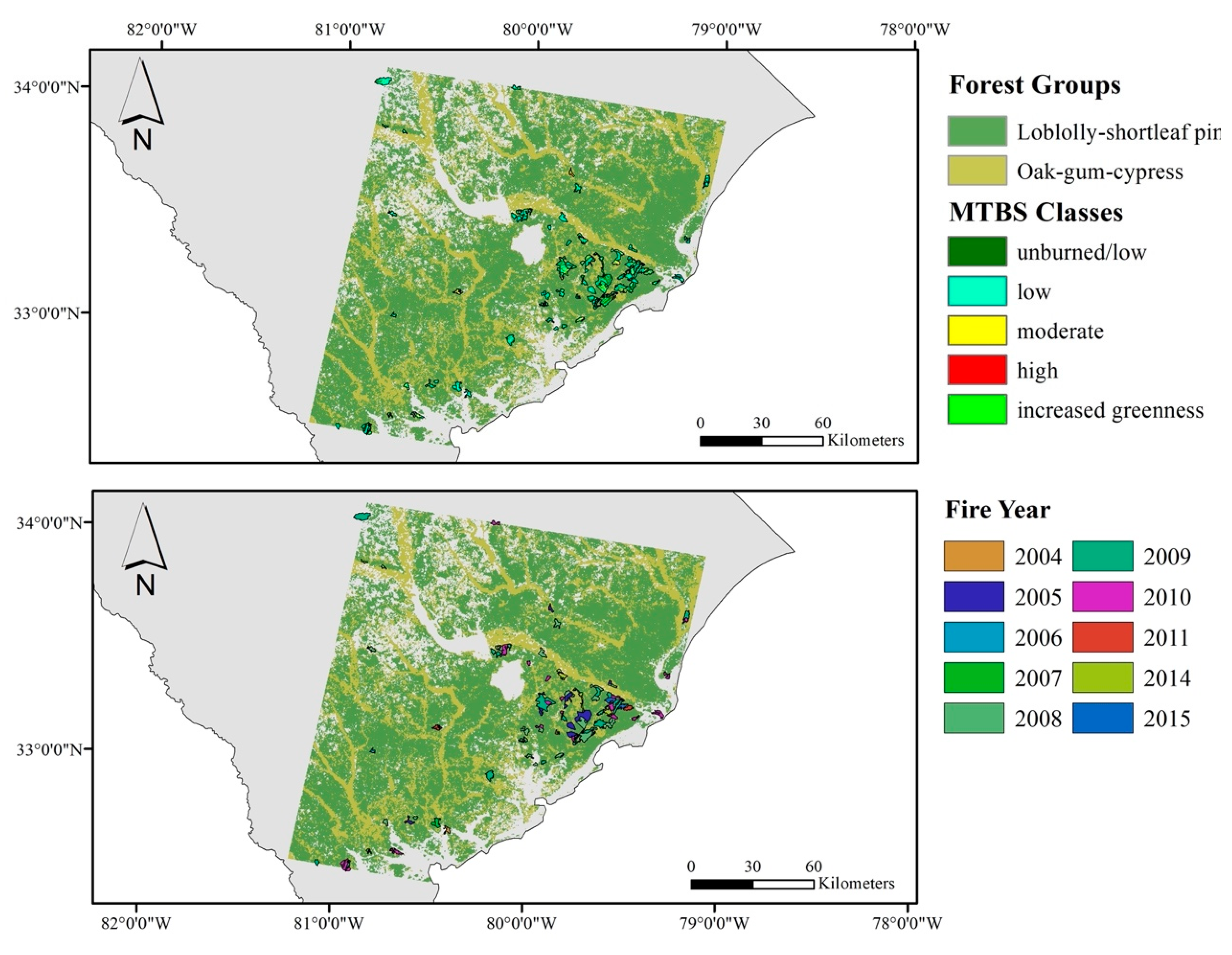
The study area selected corresponds to the Landsat scene path 16 row 37 (
Figure 1). This region is dominated by the loblolly-shortleaf pine forest group with oak-gum-cypress forests in lower-lying terrain [
27]. It falls within the Southeastern Plains and Coastal Plains ecoregions and is characterized by low elevation. This area represents one of the four focal areas in the North American Forest Dynamics (NAFD) project, which aims to better understand forest disturbance and carbon stocks in North American forests [
28,
29]. Low-severity prescribed fires are common in this region and are implemented to maintain pine-grassland ecosystems, providing ample fire perimeter and severity data that can be used to better understand differences in recovery dynamics between the two dominant forest groups [
30].
2.2. Study Data
2.2.1. Landsat Imagery
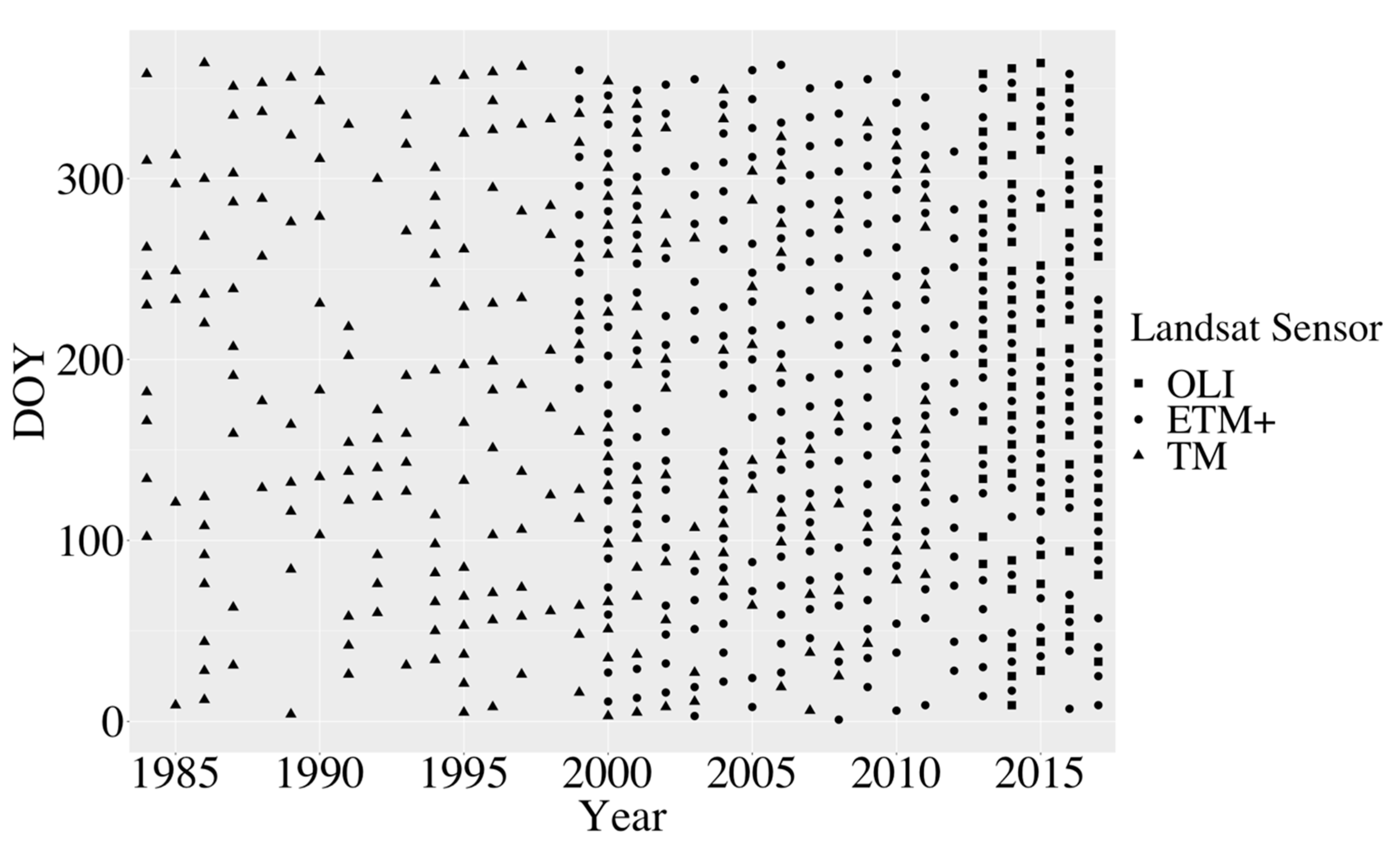
We used 660 images collected by Landsat Thematic Mapper (TM), Enhanced Thematic Mapper (ETM+) and Operational Land Imager (OLI) for the study area from 1984–2017 (
Figure 2). The Landsat Collection 1 Surface Reflectance data were downloaded from the USGS website in November 2017. Landsat TM and ETM+ are atmospherically corrected using the Landsat Ecosystem Disturbance and Adaptive Processing System (LEDAPS) algorithm (version 3.4.0) and Landsat OLI data are produced using the Land Surface Reflectance Code (version 1.4.1) [
31,
32,
33].
2.2.2. Forest Group Maps and Fire Data
U.S. Forest Service forest group maps were used to distinguish between the two dominant forest species groups in the study area (
Figure 3). These maps were derived from a variety of data, including digital elevation models (DEM), Moderate Resolution Spectroradiometer (MODIS) vegetation indices, National Land Cover Dataset (NLCD), and Forest Inventory and Analysis Data and have a spatial resolution of 250 meters [
34]. Loblolly-shortleaf pine and oak-gum cypress are two dominant forest groups in the study area.
To distinguish between burned and unburned areas, we used fire extent and severity data produced by the Monitoring Trends in Burn Severity (MTBS) program (
Figure 3). These data use Landsat-derived dNBR, the difference between pre- and post-fire NBR, which is a spectral index that combines the near infrared (NIR) and shortwave infrared (SWIR) wavelengths and is often used to identify burned vegetation [
35,
36]. MTBS data can be downloaded here:
https://www.mtbs.gov/direct-download. Because the U.S.F.S. forest group maps were generated in 2003 and past species distribution maps are unavailable, we limited our analysis to fires that occurred between 2003 and 2015 to control for changes in forest group composition that occurred prior to the creation of these maps and to ensure that the forest group maps represent pre-fire conditions.
2.3. Sample Design and Data Processing
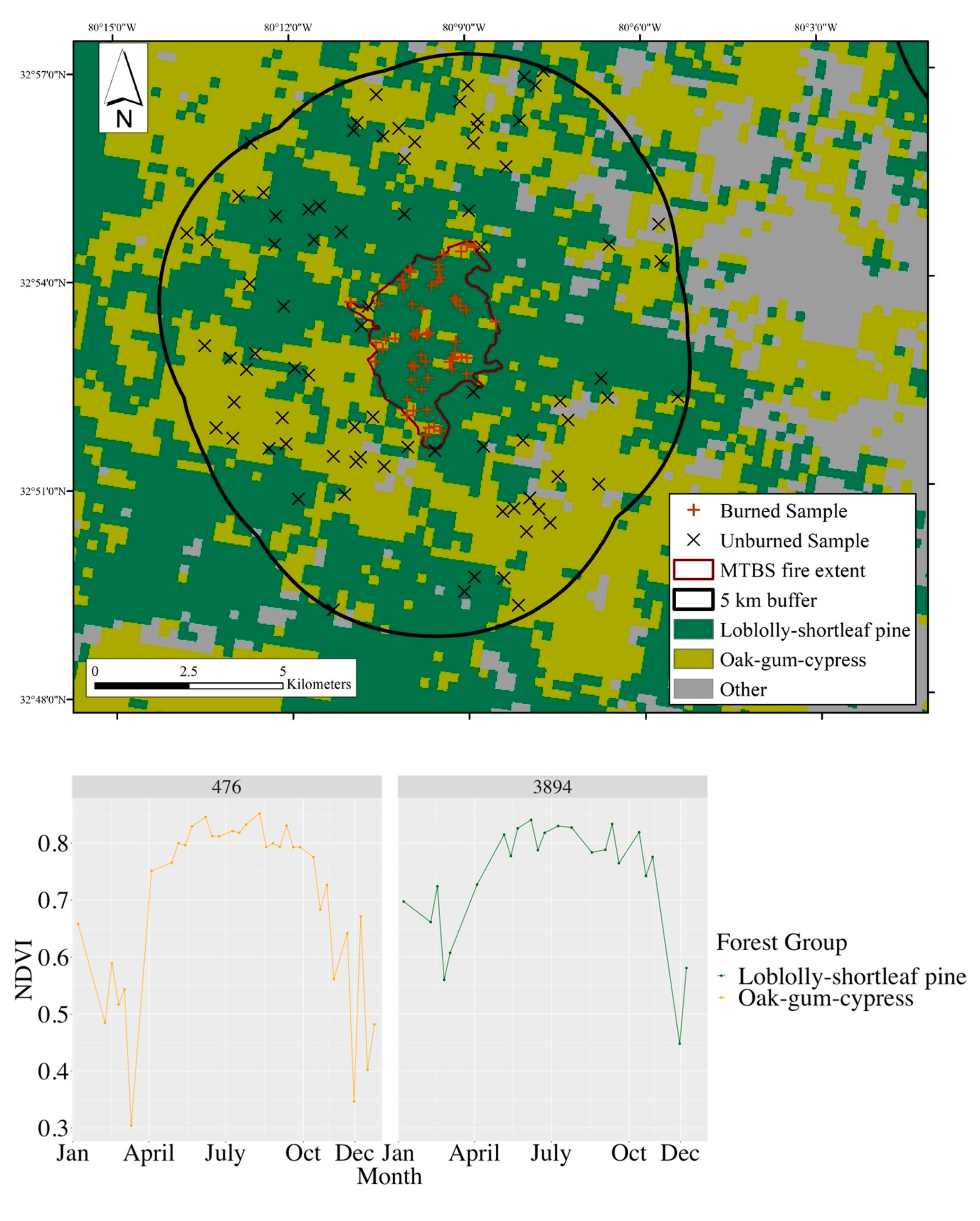
We used a pseudo control-treatment sample design, with burned forest locations as the treatment and the surrounding unburned forest locations serving as the control (
Figure 4). To better understand the differences between pre- and post-fire phenology within the burned samples, we needed to establish a baseline or “normal” set of phenology curves for forest that did not experience fire. Prior to selecting our burned samples, we removed areas that experienced more than one fire between 1984 and 2015 to reduce any confounding factors introduced by multiple burns. Using the single-burn pixels from the MTBS raster images from 2003–2015, we then sampled 1000 locations from the two forest groups, loblolly-shortleaf pine and oak-gum-cypress, for a total of 2000 burned pixels. For the control pixels, we generated 5-kilometer buffers around each of the MTBS polygons and removed all overlapping burn areas. These buffers represent unburned, control areas of similar environmental conditions to the burned samples within the fires. We sampled an equal number of pixels from the two forest groups within these buffer areas, for a total of 2000 unburned pixels.
We extracted Landsat image values and quality assurance values at the original 4000 sample locations as well as the eight surrounding pixels for phenology smoothing. These data were processed to include fire type, fire severity, forest group, Landsat image date, band number, time since or before fire, and Landsat sensor. Using the Quality Assessment (QA) bands included in Landsat Surface Reflectance product, we excluded pixels affected by instrumental or atmospheric irregularities. This method allowed us to retain all available images for the study region, while also removing cloudy and contaminated data. In total, 3698 of the original 4000 locations were retained after removing cloudy and contaminated data. We then calculated NDVI and NBR from the original Landsat values and then aggregated the data to 90 m spatial resolution using the original pixel and 8 surrounding pixels to reduce noise and retain patch-level NDVI and NBR measures even if one pixel was contaminated or cloudy on a particular date. Because the fire years ranged from 2003–2015, pre-fire Landsat observations range from one day to 31 years before the fire. Similarly, post-fire includes observations collected immediately after the fire up to 13.5 years post-fire. Note that both the burned and unburned samples include pre- and post-fire observations. For the burned samples, pre-fire curves were constructed using all Landsat observations that were collected before the fire, while “post-fire” corresponds to all observations collected after the corresponding fire. Although the unburned samples did not experience fire, they were sampled from the buffer area of a given fire. Each control, unburned sample corresponds to an individual fire and a set of burned, treatment pixels. Therefore, “pre-fire” unburned samples are observations that were taken from the unburned control area before the corresponding fire occurred. Similarly, “post-fire” unburned samples include all clear observations collected after a particular fire occurred.
In the conceptual framework used to model the pre- and post-fire NDVI (and NBR) phenology curves,
is the smooth phenology curve before the fire, which is a function of time and day of the year,
is the change in the phenology curve after the fire, and
I() is an indicator variable equal to 0 before fire and 1 for after fire. When predicting the pre-fire seasonal patterns of NDVI and NBR,
I = 0 and time after fire is null. This allows us to measure the change in phenology curve pre- and post-fire.
2.4. Harmonic Regression
To model the annual curves of NDVI and NBR derived from Landsat 5 TM, Landsat 7 ETM+, and Landsat 8 OLI pixel samples, we used a non-classical harmonic regression analysis that was developed to construct phenology curves for different land cover types in the Great Basin using AVHRR data [
16,
17]. Equation (2) gives the formula for a harmonic function with a polynomial trend, where
represents the predicted NDVI value, and
a,
b, and
c are coefficients to be estimated.
The coefficient captures the intercept and any linear, quadratic, and polynomial time trends.
The coefficients
and
capture the annual phenology variation at specific frequencies. The overall curve can be made arbitrarily flexible by making
M—the number of sinusoidal terms—very large. Unfortunately, setting
M to be large also tends toward overfitting. We modified the harmonic regression by using penalized least squares, which is a technique used in smoothing spline methods, which penalizes the magnitude of the coefficients
and
[
37] and ameliorating overfitting. The practical effect of this penalization is that it allows us to include many harmonic components, allowing us to flexibly estimate phenology curves while avoiding overfitting and spurious harmonic terms.
The formulas for the penalized least squared method are:
The penalized least squares will choose the coefficients a, b and c to best fit the data, but the harmonic terms a and b are added with a penalty to avoid “wiggliness”. The parameter controls the tradeoff between fit and wiggliness, and its effect is explored below.
Landsat scenes are imaged by the OLI, TM, or ETM+ sensor every sixteen days, making time-sensitive phenology assessments from Landsat more challenging than other sensors with high-temporal resolution, e.g., AVHRR or MODIS. In contrast to those data, however, Landsat data are collected at a 30 m spatial resolution, allowing for more precise characterization of heterogenous landscapes than is possible using AVHRR or MODIS. Harmonic regression analysis using Landsat 5 TM and Landsat 7 ETM+ data has been applied to crop phenology research [
38]; however, little work has been done to assess the usefulness of this approach in characterizing forest communities and their recovery following a disturbance using Landsat imagery.
Using the harmonic regression modelling approach, we constructed phenological models for different subsets of the Landsat data, based on forest group, burn severity, and time since fire. In constructing the initial models, we prioritized flexibility by allowing for 20 sine and 20 cosine waves every 365 days. Whereas a harmonic regression with 20 terms would normally overfit the data, the penalized regression method allows them to flexibly describe the phenology trend without introducing spurious cycles. These parameters can be adjusted for different data types or ecological systems. The traditional harmonic regression for annual NDVI is too flexible and exhibits overfitting; while it captures fluctuations in NDVI throughout the year it is also quite noisy and does not accurately reflect the average phenology of the forests in the region (
Figure 5).
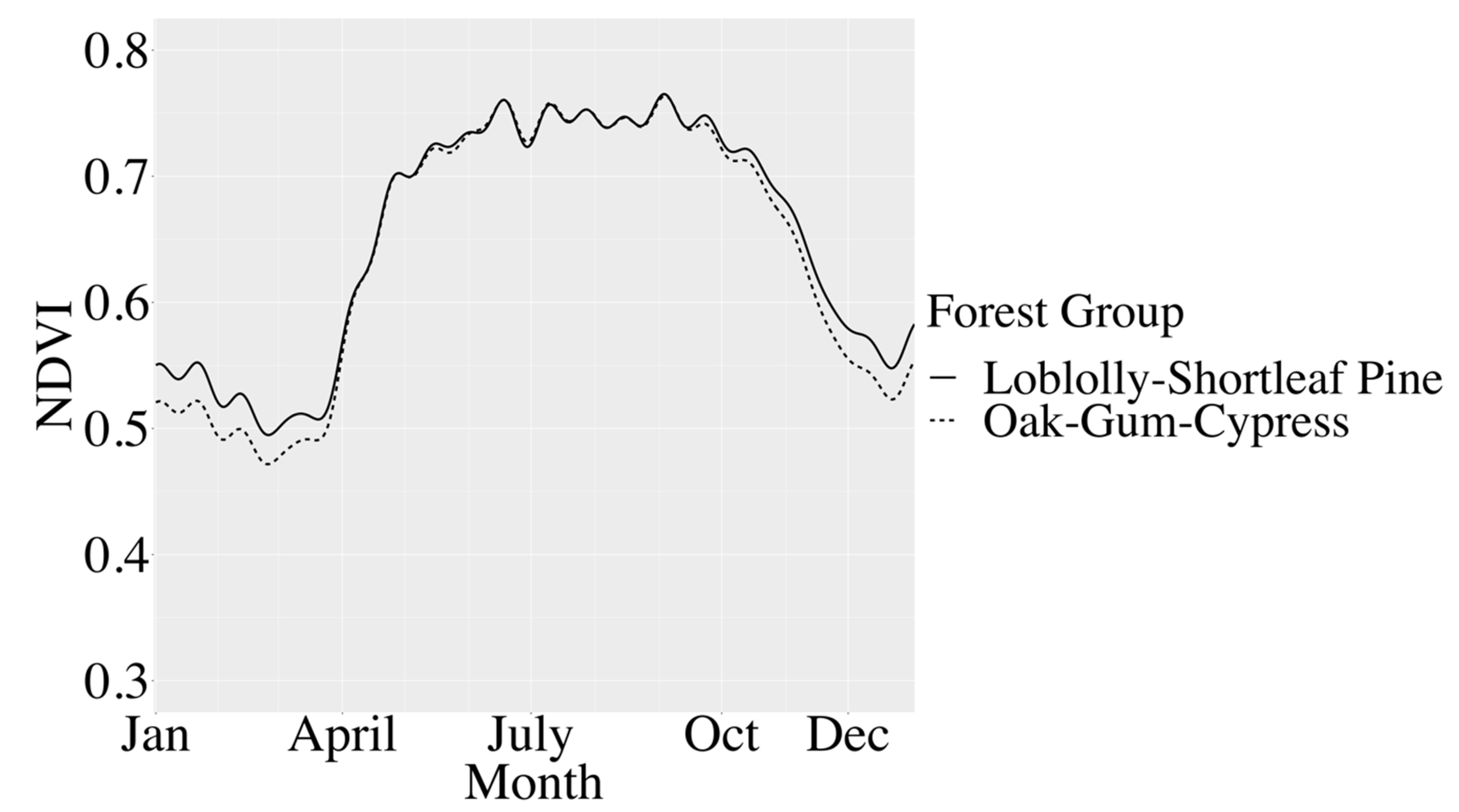
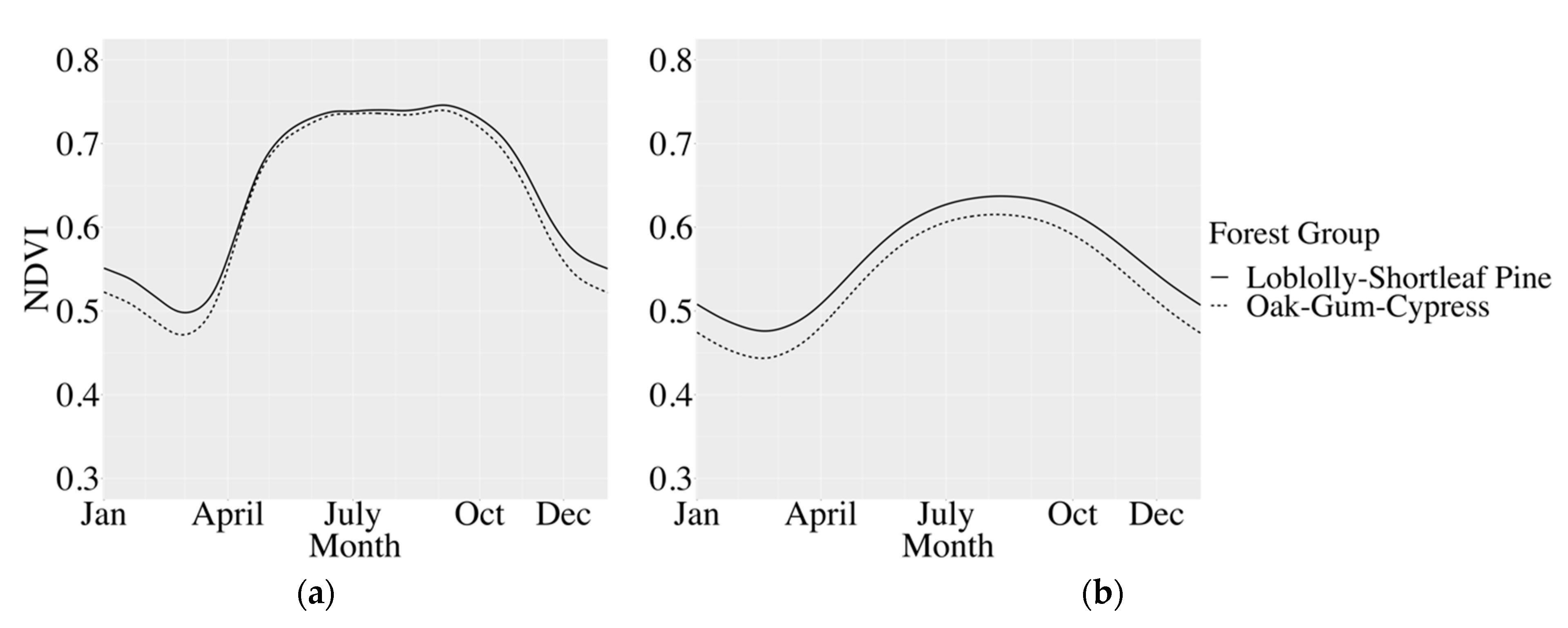
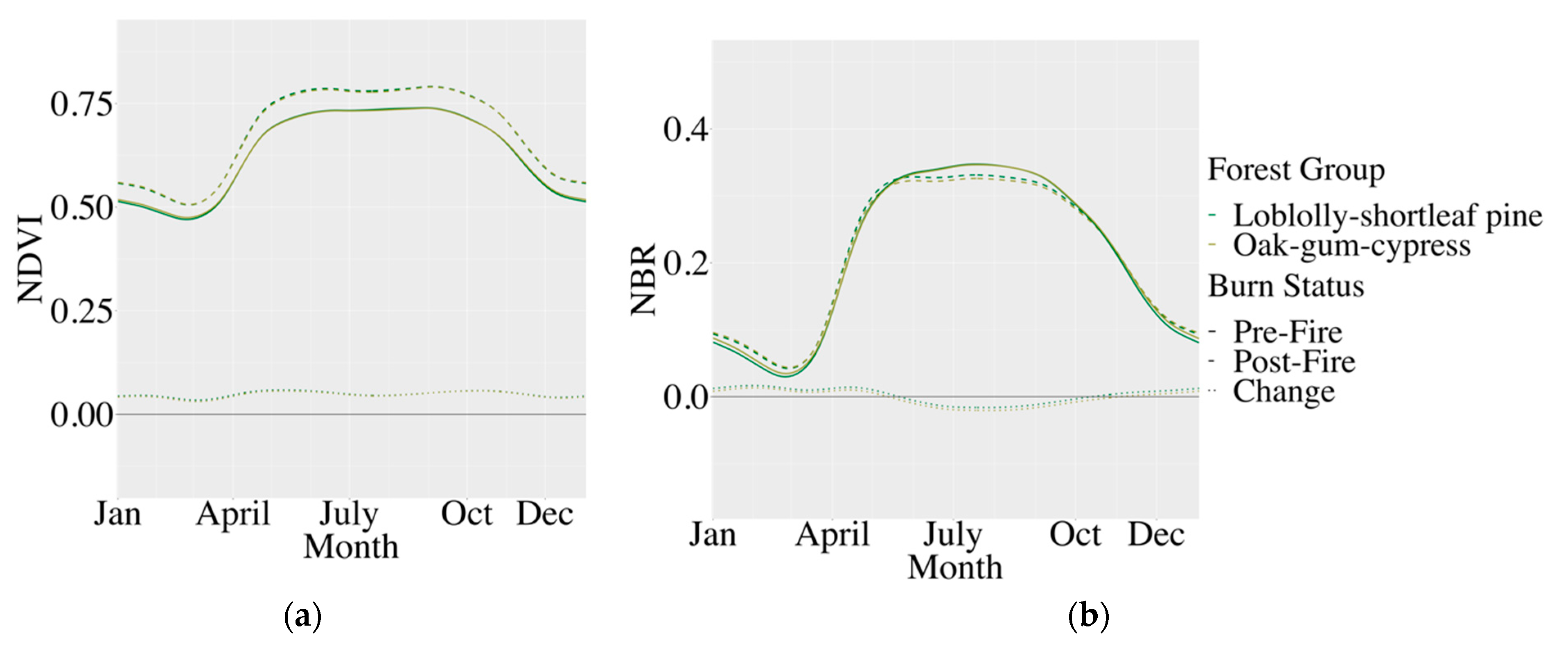
The smoothed harmonic regression model outputs for both forest groups are representative of the expected vegetation green-up phenology in the region, showing a broad summer peak greenness corresponding to the humid subtropical climate of the study area (
Figure 6a). It is important to note that the smoothing parameters must be appropriately based on expert knowledge of phenology curves; applying too much smoothing generates curves that provide little information about the seasonal patterns of the land surface being studied, also shown in
Figure 6b.
2.5. Phenology Metrics
In addition to constructing phenology curves using a smoothed harmonic regression approach, we derived several phenology metrics from the curves to compare the seasonal differences between the forest groups, pre- and post-fire, and different levels of fire severity. These metrics include the minimum and maximum predicted annual values of NBR and NDVI, the DOY on which the minimum and maximum values occur, and the timing of spring and fall senescence based on NDVI or NBR. There is no universally accepted method for defining or deriving phenology metrics, such as start of spring [
22]. However, we selected a method in which a spectral index threshold value (
SIratio) is used to identify the spring green up and start of growing season [
39]. White et al. [
39] used 50% threshold values to identify spring and onset and cessation, a value that works well with a variety of land cover types. In this method,
SIratio is the percentage of the seasonal amplitude reached at a given point in time:
To identify the DOY for spring onset and fall senescence from the phenology curves developed in this research, we used 50% threshold values. All data were processed and analyzed using R statistical software, specifically the ‘tidyverse’, ‘sf’, ‘mgcv’ and ‘raster’ packages. The penalized regression was performed using the ‘pcls’function in the ‘mgcv’ package [
37]. We have also calculated confidence intervals for all phenology curves intervals are tight and do not change the interpretation of the figures, so we have not reproduced them here.
5. Conclusions
Detecting forest change from space requires the comparison of spectral signals over time. Classical techniques have relied on the comparison of a few images. Spectral signals can change in many ways, for example the timing and slope of greenup and senescence can change or the timing of the peak NDVI can shift. Landscape change can display in the spectral signature as a changing phenological curve, and not just a change in levels represented by a small selection of images.
In this paper, we have presented a simple curve-fitting method that captures these phenological changes using the entire Landsat image stack, rather than just few images. Since phenology is seasonal, we have use curve-fitting based on harmonic regression. All curve-fitting methods can suffer from overfitting, and previous effort at harmonic fitting have addressed this be including just a few low frequency components. These are a good start, but they do not represent phenology well because plant phenology is not a precise sinusoidal wave. We used the statistical technique of penalized regression to more flexibly fit a curve to the image stack while avoiding overfitting. Our method relies on well-established packages from the R statistical software and is accessible from current desktop computers. These methods could also be implemented using Google Earth Engine, which does not require the user to download all Landsat images for analysis and has been used for harmonic modeling with remote sensing data [
6,
49].
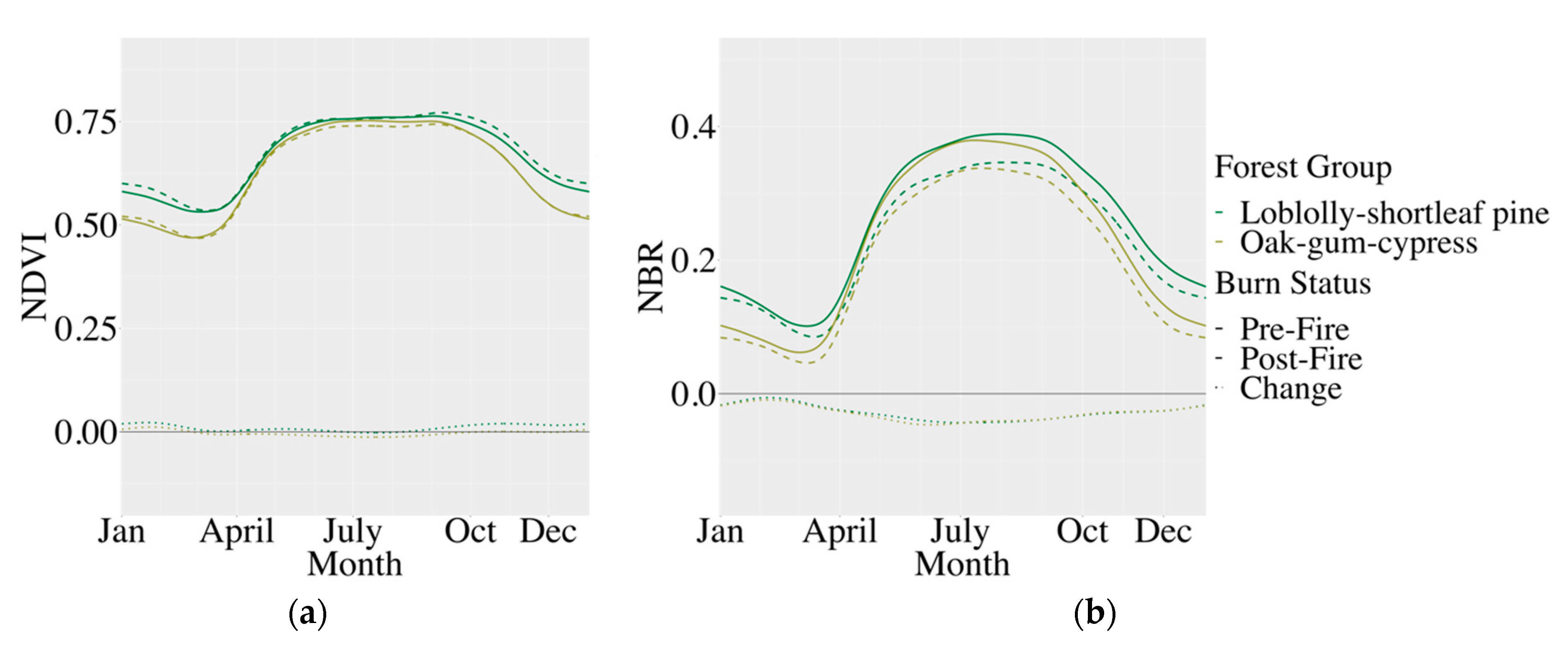
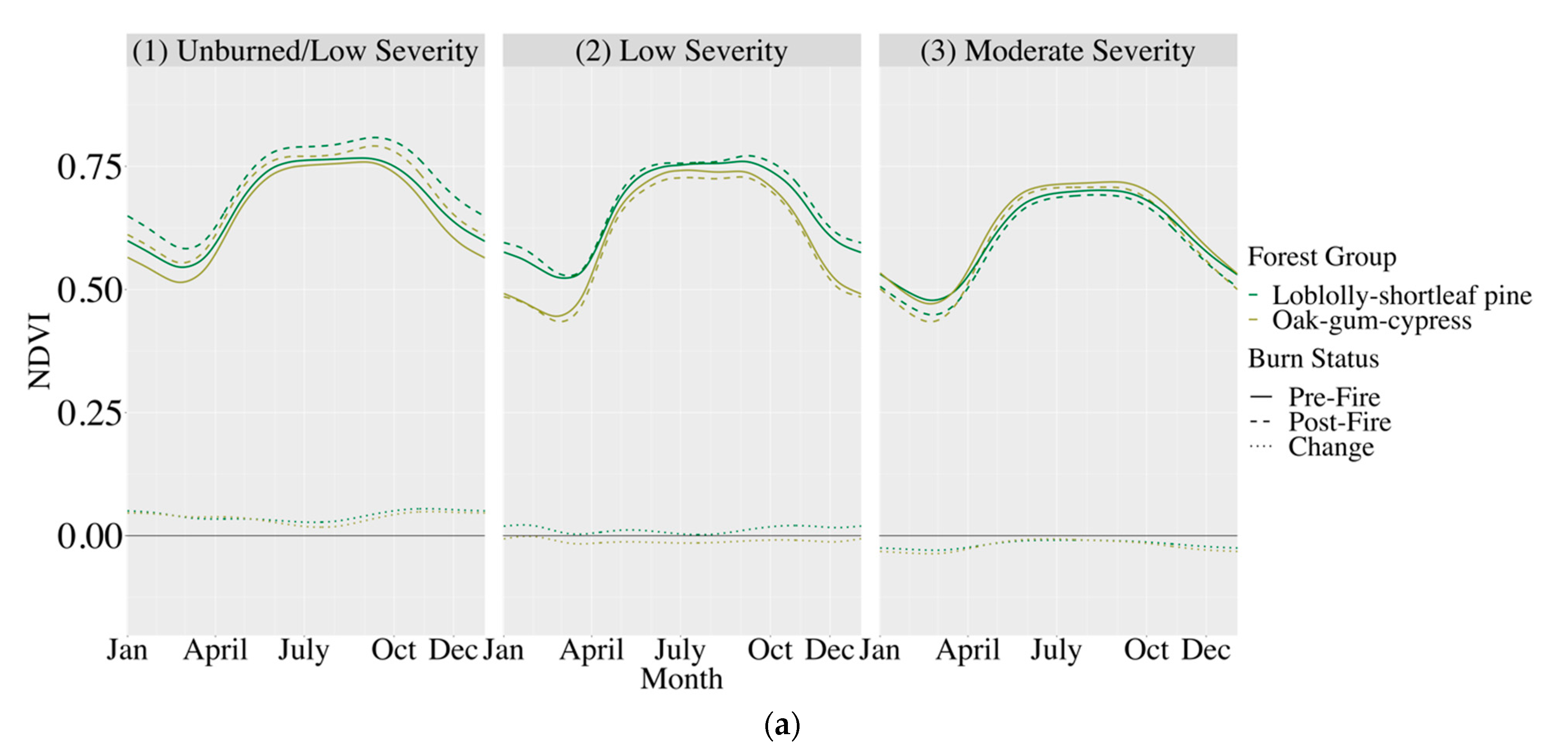
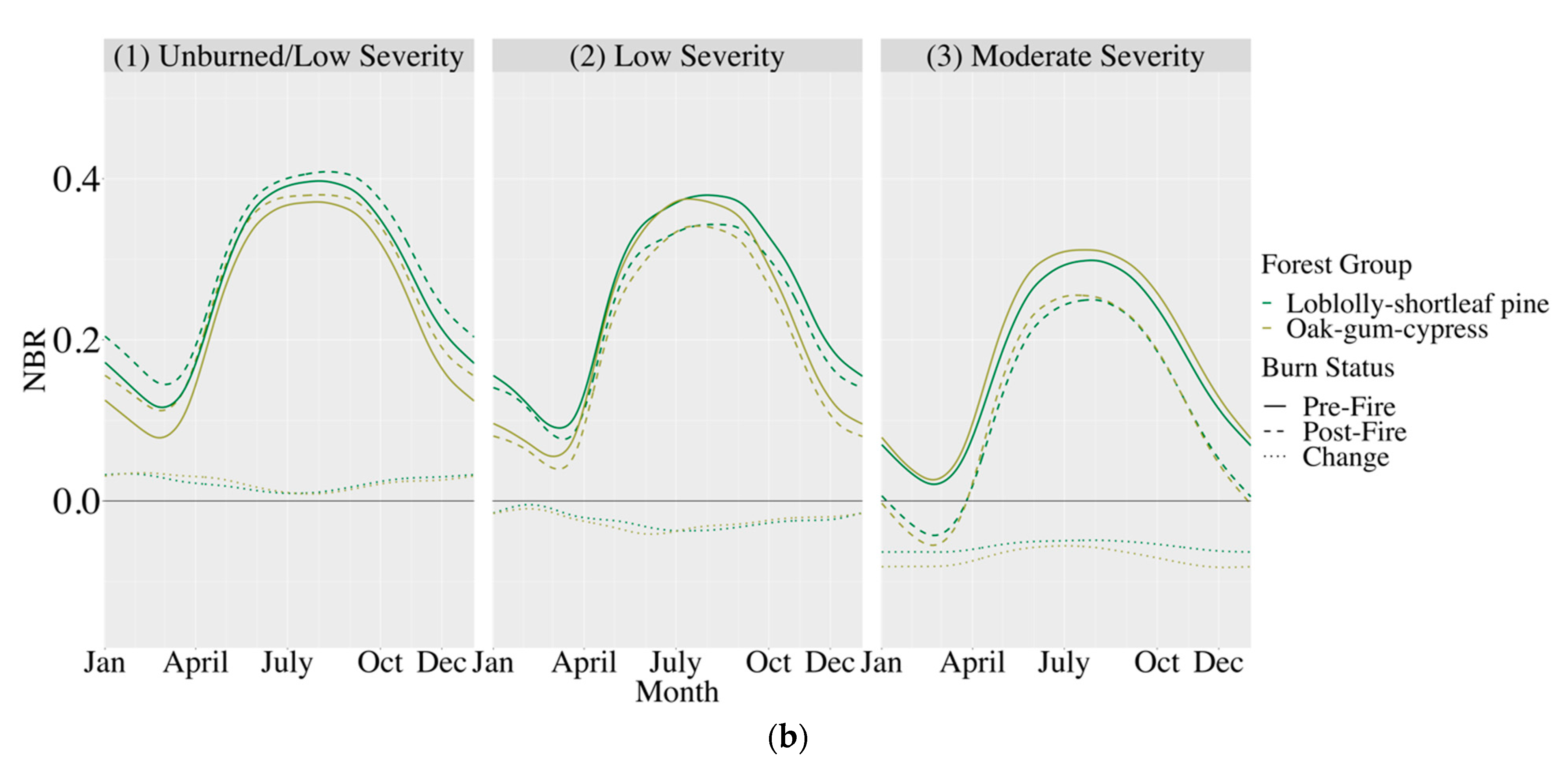
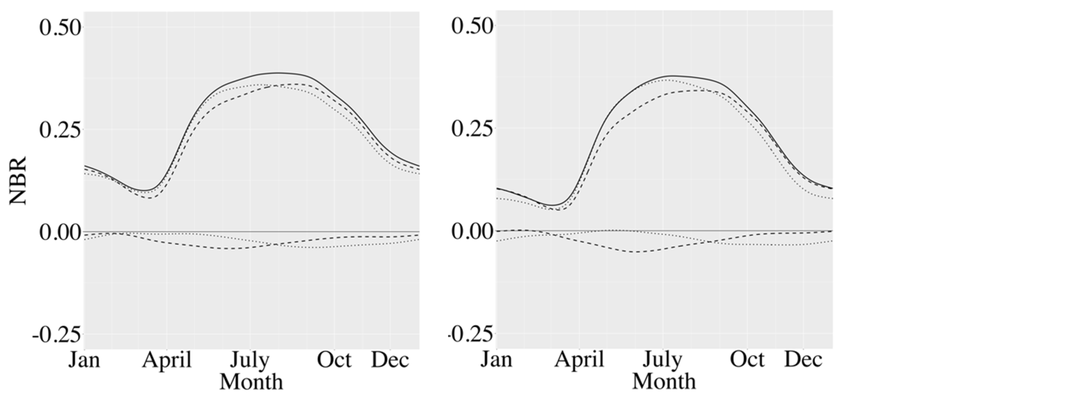
Our results demonstrated that Landsat NDVI and NBR phenology curves in loblolly-shortleaf pine differed from the phenology curves of oak-gum-cypress. As expected, post-fire NBR phenology curves in both forest groups showed a decrease from pre-fire levels, with some variability in the magnitude of that decrease throughout the year. There was no difference between the forest group phenology curves of the unburned samples. While additional analysis is necessary to understand the differences observed between phenology patterns of the burned and unburned samples, a potential ecological explanation for this pattern could be that the lack of fire for the study period has led to the homogenization of forest groups, with the loblolly-shortleaf pine transitioning into a deciduous forest type. Although more work is needed to refine the uncertainty measures of these phenology curves, the current results suggest that deriving phenology curves from Landsat data is a feasible approach for better understanding forest recovery after fire.
These findings provide information about successional patterns and differences between forest groups following fire, which are key components of forest health and aid in forest management decisions. Phenology metrics and patterns derived from remote sensing imagery with relatively fine temporal yet coarse spatial resolution (i.e., MODIS and AVHRR) have been used to characterize patterns in disturbance and recovery cycles across broad spatial scales. However, forest disturbance-recovery dynamics are often spatially heterogenous, with important changes occurring across gradients at finer spatial scales than can be detected by these sensors. The methods we present allow researchers to more reliably monitor forest dynamics at finer spatial resolutions than has been traditionally feasible. Using the entire Landsat stack, scientists can develop richer and more sensitive measures of change. These measurements will contribute to the improvement of continuous sensing of forest landscapes.


