Abstract
There are two useful methods of current measurement based on synthetic aperture radar (SAR): one is along-track interferometry (ATI), and the other is Doppler centroid analysis (DCA). For the ATI method, the interferometric phase must be accurate enough for ocean current measurements. Therefore, the space-varying of phase imbalances along the range, caused by antenna phase center position error, attitude error, antenna electronic miss pointing, antenna pattern mismatch, and other reasons, cannot be ignored. Firstly, this paper mainly analyzes the above possible factors by using real GF-3 ATI data and error model simulation results. Secondly, the ocean current has been preliminarily measured by the ATI method and the DCA method, using CDOP model, based on the GF-3 ATI data of the ocean scene near Qingdao, China, which is up to around −1.45 m/s. The results of the two methods are in good agreement with the correlation coefficient of 0.98, the mean difference of −0.010 m/s, and the root mean squared error (RMSE) of 0.062 m/s. Moreover, by comparing with the current measured by high-frequency surface wave radar (HFSWR), the correctness of the analysis is further proved.
1. Introduction
The study of ocean currents is an important part of ocean dynamics and is of great significance to humans working on the sea and in coastal areas. Synthetic aperture radar (SAR) is a high-resolution imaging radar that can observe the Earth for all weather and all time. Since the first spaceborne SAR, SeaSat, was launched successfully in 1970, SAR has shown irreplaceable ocean observation advantages. According to previous studies, SAR can accurately measure ocean currents with high spatial resolution. Two methods of SAR current measurement are produced based on the characteristic that a target moving relative to the radar will make a Doppler frequency shift proportional to the speed. Goldstein and Zebker [1,2] proposed the concept and basic theory of ocean currents obtained by ATI-SAR in 1987 and demonstrated for the first time the ability of ATI-SAR to measure surface currents in San Francisco Bay, Mission Bay, and San Diego Bay in 1989. Delwyn Moller and Stephen J. Frasier [3] combined the in site acoustic Doppler current profiler (ADCP) measurement to explain how to extract the surface current from the interferometric phase and confirmed the analysis model of the directional propagation of Bragg resonance waves in 1998. Romeiser and Thompson [4] proposed an efficient model for the simulation of Doppler spectra and ATI signatures based on Bragg scattering theory in a composite surface model approach in 2000. In 2003, Duk-jin Kim [5] reviewed the relationship between the phase difference measured by SAR and the average Doppler frequency and proposed a method to remove the Bragg wave phase velocity based on the C and L dual-band ATI-SAR technology, since the proportions of C-band and L-band Bragg wave components propagating in different directions are approximately equal. In 2005, Romeiser et al. [6] used the data obtained during the Space Shuttle Radar Topographic Mapping Mission (SRTM) in February 2000 through additional along-track antenna separation of 7 m to first analyze the ocean current measurements by ATI-SAR. Comparing the currents in the Wadden Sea area of the Netherlands measured by ATI-SAR with the results of the numerical circulation model KUSTWAD, the correlation coefficient was as high as 0.6, and the root mean squared error was within 0.2 m/s. In 2010, Romeiser et al. [7] showed preliminary results based on actual TerraSAR-X ATI data. The results obtained by using TerraSAR-X Aperture Switching (AS) mode in the Elbe River mouth area were consistent with the UnTRIMresults. It is believed that the typical current measurement accuracy of TerraSAR-X ATI under the effective spatial resolution of 1000 m can reach a performance of 0.1 m/s.
Chapron [8] first proposed the Doppler centroid analysis (DCA) method in 2005. Rouault et al. [9] used the DCA method to monitor the Agulhas current in 2010 successfully. The current inverted by the DCA method can replace the altimeter measurement result. In 2010, Hansen et al. [10] verified that the sea surface velocity retrieved by the SAR DCA method has an accuracy of 0.05 m/s at a resolution of 10 km. In 2013, Romeiser et al. [11] analyzed two TanDEM-X interferograms with effective baselines of 25 m and 40 m obtained in the Pentland Firth in Scotland and compared with the TerraSAR-X dual-receiving antenna (DRA) mode interferogram with an effective baseline of 1.15 m and the velocity field of single antenna data from the same scene obtained by DCA. Under the same measurement accuracy conditions, compared with DRA mode, the spatial resolution of the currents obtained from the TanDEM-X interferogram is higher than that of DRA mode. The DCA-based currents are less accurate than the ATI-based ones, but close to short-baseline ATI results in quality.
However, the interferometric phases are not simply proportional to the velocities of the ocean currents because the average surface current does not completely determine the average Doppler of the radar backscatter on the sea surface, but also includes the large-scale wave orbit velocity and the phase velocities of Bragg-resonant waves [3]. The empirical models can be used to remove each component to extract the ocean currents. Of course, only the line-of-sight (LOS) velocities of ocean currents can be obtained, but the direction of ocean currents cannot be determined.
On 10 August 2016, Gaofen-3 (GF-3) was successfully launched into space at the Taiyuan Satellite Launch Center. GF-3 is China’s first C-band full-polarization synthetic aperture radar (SAR) imaging satellite with the highest resolution of 1 m. GF-3 has 12 imaging modes, covering traditional strip imaging mode, scanning imaging mode, wave imaging mode, and global observation imaging mode for marine applications [12]. It is the SAR satellite with the most imaging modes in the world. Besides, GF-3 also carried out multiple ATI test missions in 2018 and 2019, imaging by dual-receiving, and obtained two fine strip-map (FSI) mode images of the same scene with a time lag of milliseconds, which used an effective along-track antenna separation of 3.75 m. We analyzed the dual-channel space-time variability of phase imbalance in GF-3 ultra-fine strip-map (UFS) mode through simulation and a large amount of actual data [13], considering that the dual-channel space-time variability of phase imbalance is attributed to the antenna phase position error and phase mismatch of the antenna pattern.
This paper starts with Section 2, which introduces the current measurements method based on GF-3 ATI data. Through the GF-3 imaging geometric model with errors, all the error sources are analyzed, and a calibration method of phase imbalance is introduced. After describing and analyzing the possible causes of phase imbalance in GF-3 ATI mode by real data processing, Section 3 presents the ocean current obtained by the GF-3 ATI data. Section 4 summarizes the results of experiments with some discussion and research perspectives for the future, and Section 5 gives the conclusions of this paper.
2. Ocean Current Measurement Method Based on GF-3 ATI Data
2.1. Model of GF-3 ATI Ocean Current Measurement
The GF-3 ATI-SAR system applies two antennas arranged along the track direction to acquire the echo reflected by the same observation area. The interferometric phase of the echo signals acquired by two channels is proportional to the target’s speed in the LOS of the SAR. The geometric model in the azimuth-slant range plane of the GF-3 ATI system is shown in Figure 1, which has two along-track receiving apertures. The satellite platform’s velocity is , and the closest slant range from the satellite platform to the center of the observation scene is . The phase center of the entire antenna, , transmits pulses, while the dual-channel antenna phase centers, and , receive the scene echo simultaneously. The moving target velocity is decomposed into the radial velocity and the azimuth velocity . Ideally, that is, the two receiving apertures are absolutely the same, and the total antenna length is , so the phase center spacing between beams can be written as . Assuming that the azimuth moment equals zero, the coordinate of the entire antenna phase center in the azimuth-slant range plane is , and the actual phase center coordinates of each sub-beam are , where
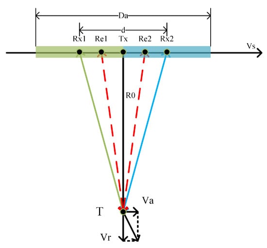
Figure 1.
Geometric model in the azimuth-slant range plane.
After compensating for a constant phase, the th channel’s echo can be equivalent to the echo spontaneously sent and received at the equivalent phase center (EPC). Then, the coordinate of the equivalent phase center of the th channel is , where:
where B represents the effective along-track interferometric baseline. Specifically for GF-3 ATI mode, m. Therefore, GF-3 ATI mode has a 3.75 m along-track interferometric baseline. The two equivalent single-channel echo signals are denoted by and , respectively. According to [14,15,16], can be obtained by through a certain time shift and phase shift. For a stationary target, the relationship between and can be expressed as follows:
where .
It is reported that the radial velocity of a moving target can be directly calculated by the interferometric phase [17,18,19]. After matching, the interferometric phase between channels can be expressed as follows:
As described in Equation (5), the two images’ interferometric phases are proportional to the radial velocity of the target at the corresponding position, and the interferometric phase for a stationary target is zero.
Yet, it should be pointed out that the radial velocity does not reflect the real ocean current. Since the SAR imaging mode of the sea surface is extremely complicated and includes the components in the LOS velocity of the sea surface scatterer of different scales in the sea surface scattering unit, then can be derived as,
where is the radar incident angle, represents the contribution of the ocean current, represents the contribution of the sea surface wind, represents the contribution of the large-scale wave orbital velocity, and denotes the contribution of the phase velocities of the Bragg-resonant wave components. The large-scale wave orbital velocity changes periodically, and the average value is zero, which can be removed by the neighborhood average. The contribution of sea surface wind can be calculated by using the CDOPmodel, which is an empirical geophysical model function for predicting the Doppler frequency shift of sea surface wind proposed by Mouche et al. [20,21].
where is the incidence angle in degrees, is the wind direction with respect to the antenna look angle in degrees, is the wind speed, and represents the polarization. For the details of the formula, please refer to [21]. The phase velocities of Bragg-resonant waves can be removed by empirical models, given by [3,22]:
where g is the gravitational acceleration constant, k is the Bragg wave number, is the sea surface tension, and is the seawater density. The speed measured by the radar is determined by the ratio of the spectral density of the forward waves and the backward waves in the resolution unit.
Among them, and represent the contribution ratio of forward and backward Bragg spectral density to radar echo, respectively. Generally speaking, the following model and wind information can be used to estimate the contribution of Bragg wave phase velocity to radial velocity.
where n is usually 2∼5; for C-band SAR, .
2.2. Error Analysis of the Phase Imbalances between Channels
The phase imbalances between channels for ATI-SAR are caused by many factors, such as the radar electronic system, the phase mismatch of the antenna pattern, satellite attitude errors, antenna electronic miss-pointing, antenna phase center position errors, sampling time delay error, and target elevation [13]. Therefore, the interferometric phase directly obtained from the two SAR images cannot truly reflect the Doppler information of the radar irradiation area. Firstly, the radar electronic system error will introduce constant phase errors. Secondly, due to the attitude error and antenna electronic miss-pointing, the squint angle will appear in SAR imaging, which directly leads to the inconsistent distance between the center of dual receiving channels and the target. Thirdly, the antenna phase center position of each receiving channel may change due to installation errors, thermal deformation, etc. Therefore, the antenna phase center position errors and satellite attitude errors will cause an additional cross-track baseline, which will produce phase imbalances that vary with the slant range and target elevation. Finally, sampling time errors between the two channels caused by inconsistent synchronous circuits and analog-to-digital devices will also lead to a dual-channel phase imbalance. In the range-Doppler domain, phase imbalance can be expressed as [23]:
where ∠ stands for calculation angle operation, is the Doppler centroid frequency, which can be measured by real data, is the range frequency, is the sampling time delay, and is the phase imbalance caused by the baseline error and constant phase imbalance between channels. In short, after compensating the sampling time delay error, the space-varying phase imbalance may be caused by squint imaging, baseline error, and the phase mismatch of the antenna pattern.
Although GF-3 ATI-SAR is a vertical side-looking imaging system, due to satellite attitude error, antenna electronic miss-pointing, and other reasons, it will be actually squint imaging. The geometric model with baseline error under the condition of squint imaging is shown in Figure 2, where is the squint angle.
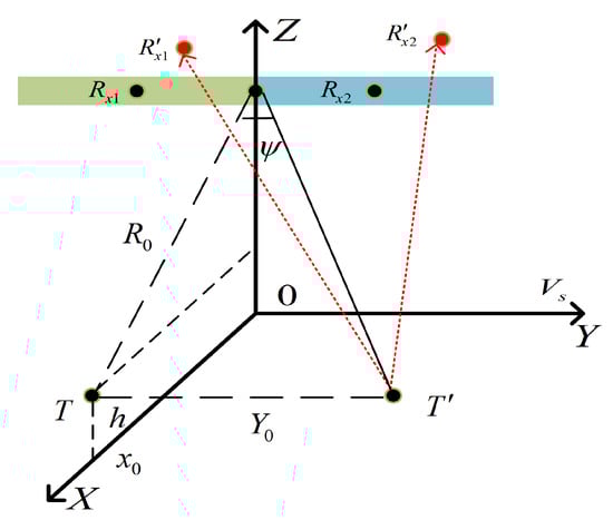
Figure 2.
The geometric model with baseline error under the condition of squint imaging.
In the case of squint imaging with an antenna baseline error, which is , the distance from the actual antenna receiving center to the corresponding point T’ can be expressed as:
The phase imbalance between channels in the case of squint imaging caused by baseline error can be expressed as [13,24]:
Let , , and . When , that is at the time of the Doppler centroid, the phase imbalance can be expressed as:
where is the look angle, and . It can be seen from the geometric relationship that and vary with range. Therefore, and will change approximately linearly in range caused by squint imaging and baseline error.
Firstly, only considering the baseline error caused by the antenna phase center position error, that is when the squint angle is zero, the phase imbalance and the measured radial velocity error can be expressed as:
Performing the Taylor expansion of Equation (20) and ignoring higher order terms,
where and represent the baseline component parallel to the slant direction and the baseline component perpendicular to the slant direction caused by the antenna phase center position error, respectively. Define , where and represent the look angle of the image far range and near range, respectively. Obviously, the error increases with the increase of . On the one hand, must reach an accuracy of 0.1 mm to make the constant term of velocity error less than 0.1 m/s. On the other hand, four sets of look angle parameters of GF-3 FSI imaging mode, which are shown in Table 1, are selected to calculate the maximum allowable , ensuring that the calculated radial velocity along the range is less than 0.1 m/s in GF-3 ATI mode. For example, when GF-3 imaging is at the antenna beam of 162, the antenna baseline error component caused by antenna phase center position error must be less than 0.1 mm, and component must be less than 1.58 mm, where the look angle under the center is 18.22, . Moreover, and must be in the quadrilateral surrounded by the four constraint curves shown in Figure 3a, so that the radial velocity measurement error caused by antenna phase center position error can be ignored for current measurements.

Table 1.
GF-3 radar parameters.
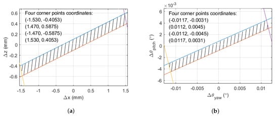
Figure 3.
Under the condition that the accuracy of radial velocity measurement is 0.1 m/s and the beam code is 162, the allowable range of antenna phase center position error and attitude error is obtained. (a) Allowable antenna phase center position error range: the values of and must be located in the area of diagonal line in the figure. (b) The allowable range of attitude error without considering squint angle: the values of and must be located in the area where the oblique line is drawn in the figure.
Secondly, considering the baseline error caused by the attitude error and ignoring the squint angle caused by it, the position error of the antenna phase center introduced by the attitude error can be expressed as:
where is the pitch error and is the yaw error. Similarly, and must be within a quadrilateral surrounded by four constraint curves, which is shown in Figure 3b. Therefore, attitude control and antenna phase center position must be sufficiently accurate in ocean surface radial velocity measurement. Moreover, it can be found that the accuracy requirement of is higher than that of , and the accuracy requirement of the pitch angle is higher than that of the yaw angle. Generally speaking, when and is out of range, the phase imbalance of the antenna in the ocean scene needs to be eliminated by using the phase imbalance of the land scene.
Thirdly, the phase imbalance caused by the baseline error will be affected by the target elevation from Equation (17). For the spaceborne ATI-SAR system, is generally in the order of mm and in the order of several hundred kilometers, so the space-varying of phase imbalance caused by target elevation is too small to be ignored. Therefore, the target elevation factor is not the main cause of phase imbalance in range for the spaceborne ATI-SAR system.
Finally, the image width of GF-3 FSI mode is 50 km, that is to say, the image width of GF-3 ATI mode is also 50 km. Under the condition that the width of the image remains unchanged, the phase imbalance between the near range and the far range of the image changes with the central look angle of the scene is shown in Figure 4, which leads to the baseline error caused by the maximum attitude control errors of GF-3, which are shown in Table 2. With the increase of the central look angle of the scene, the influence of the space-varying of phase imbalance on radial velocity measurements will become smaller.
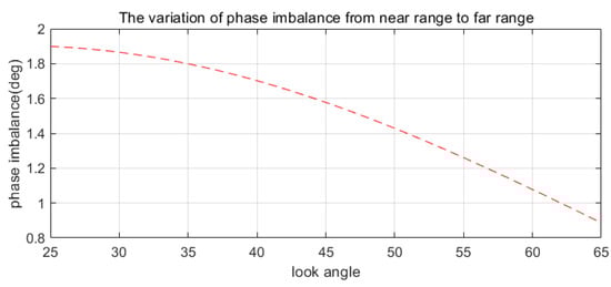
Figure 4.
The change of phase imbalance in range caused by maximum attitude control errors of GF-3.
Table 2.
The max attitude control errors of GF-3.
2.3. Calibration Method of Phase Imbalance between Channels
For phase imbalance calibration of azimuth multi-channel (AMC) SAR, researchers have done much research and put forward many methods such as the orthogonal subspace method [25], the signal subspace comparison method [26], etc. However, the space-varying of phase imbalance error is not considered. In the SAR instrument with joint XTI-ATI mode, the known elevation and velocity of land or ships are needed for phase imbalance calibration. In [27], the phase imbalance introduced by surface height was removed by the high precision DEM information, and the phase trend in range was removed using a second-order polynomial fit. In [28], the phase imbalance was calibrated by using the ships as the reference of the known velocity. However, since the satellite attitude and velocity will change with the azimuth time and the antenna phase center position error and antenna phase pattern are unknown, the cross-track baseline error is uncertain. Therefore, the phase imbalance cannot be calculated by a theoretical formula. According to [29,30], there is a method to calibrate the trajectories of SAR systems using the multisquint phase. In this paper, a method based on SAR echo data without the actual satellite state was used to remove the space-varying of phase imbalance. Through proper block processing in the azimuth and range, the echo signal delay and phase imbalance between two channels are solved by using the least squares method in the Doppler frequency domain, where the land scene is needed as a reference.
For stationary targets, the dual channel echo signal satisfies the following formula in the Doppler frequency domain [14]:
where is the Doppler frequency and represents the phase imbalance between channels caused by various errors. is a linear function of the Doppler frequency , where the coefficient of the first term represents the time delay of the received echo of the two channels and the constant term represents the phase imbalance of the two channels. Therefore, image registration and moving target velocity measurement can be carried out directly by using the calculated , without knowing the exact along-track interferometric baseline and satellite velocity. The steps of phase imbalance error calibration are shown in Figure 5. The process flow is as follows:
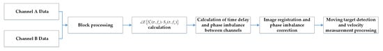
Figure 5.
Phase imbalance calibration flowing diagram.
(1) According to the appropriate block size and step size, the dual channel images are divided into blocks along the azimuth and the range. The premise of this is to ignore the space-time variation of the phase imbalance between channels in each block.
(2) The azimuth FFT is applied to each block image of the dual channel, and the corresponding conjugate multiplication is performed in the Doppler frequency domain and averaged along the range. Finally, the phase change along the Doppler frequency is obtained.
(3) The curve near zero frequency is intercepted and solved by the least squares method to obtain the time delay and phase imbalance between each small piece of dual channel data, which is to avoid the influence of high-frequency noise.
(4) Image registration and phase imbalance calibration are performed by using the time delay and phase imbalance of dual channel data calculated in the previous step.
(5) Finally, further moving target detection and velocity measurement are carried out.
For example, the change of with is shown in Figure 6, which is calculated by real GF-3 ATI data. In addition, due to the existence of high-frequency noise and squint imaging, the Doppler centroid is not zero; the phase is not strictly symmetrical about zero frequency in Doppler frequency domain and loses its linear characteristics at high frequency. In order to avoid high-frequency noise, the curve in the red box is intercepted and fitted linearly. The time delay between channels is −0.491 ms, and the phase imbalance is −162.9 by using the least squares method. Then, the phase imbalance and time delay between the dual channels of the whole SAR image can be obtained by processing each small block of the SAR image along the azimuth and range.
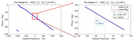
Figure 6.
The change of with .
3. Data Processing and Interpretation
Since GF-3 ATI mode is an experimental mode, there are only a few sets of data obtained in 2018, 2019, and 2020, respectively. Moreover, since the backscattering coefficient of the land scene is stronger than that of the ocean scene, the SAR echo is likely to be saturated, and then, the amplitude and phase information of the echo cannot reflect the real situation. According to the auxiliary data of these GF-3 ATI data, we can analyze the degree of saturation. In order to avoid the influence of data saturation on the experimental results, only three sets of GF-3 ATI data shown in Table 3 can be selected for GF-3 ATI mode phase imbalance analysis and moving target velocity measurement. The first set of data and the second set of data are all land scenes whose interferometric phase will be zero without any errors, which are very suitable for phase imbalance analysis. In fact, the second set of data was obtained by reorganizing an experiment with the imaging parameters of the first set of data to verify whether the phase imbalances of GF-3 ATI mode are systematic errors or random errors. The third set of data was specifically designed for the GF-3 ATI current measurement experiment.
Table 3.
GF-3 radar parameters.
3.1. Analysis of Channel Phase Imbalance
In order to analyze the source of dual channel phase imbalance in GF-3 ATI mode and verify the effectiveness of the phase imbalance calibration method mentioned in Section 2.3, the first set and the second set of GF-3 ATI data were processed and analyzed in detail, where each set of data had 15 scenes. As shown in Figure 7, the phase imbalances of the two sets of GF-3 ATI data clearly changed monotonously with the range, which changed about and , respectively, from near range to far range. Therefore, it is necessary to analyze and remove the phase imbalance in range for the high-precision current velocity measurement.
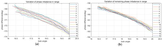
Figure 7.
The space-varying of phase imbalances in range. (a) The first set of GF-3 ATI data; (b) the second set of GF-3 ATI data.
3.1.1. Sampling Time Delay
The dual-channel sampling time delay can be obtained by analyzing the inner calibration data. Firstly, the pulse compression is carried out for the dual-channel inner calibration signals, and then, the sinc function interpolation algorithm is adopted to resample the signals after pulse compression. Finally, the time difference between the peak amplitude points of dual-channel signals is compared to obtain the sampling time delay error. A shown in Figure 8, it is obvious that there is a certain time delay between the Channel A signal and the Channel B signal of the first set of data and the second set of data. Furthermore, the range position of the image of Channel A relative to the image of Channel B will become inconsistent, caused by the sampling time delay, antenna phase center position error, and attitude error. The position offset of the dual-channel image in the range can be obtained by the correlation algorithm for image registration [31,32], which is represented by . After calculating, the position offsets in range caused by each error are shown in Table 4. The range position offsets of the first set of GF-3 ATI data and the second set of GF-3 ATI data are −0.0364 pixels and −0.0326 pixels, respectively. The range sampling time delays of the first set of GF-3 ATI data and the second set of GF-3 ATI data are −0.266 ns and −0.249 ns, respectively, so the corresponding image range position offset is −0.0355 pixels and −0.0332 pixels. Therefore, the range image position offsets caused by antenna phase center position error and attitude error are only −0.0009 pixels and 0.0006 pixels.
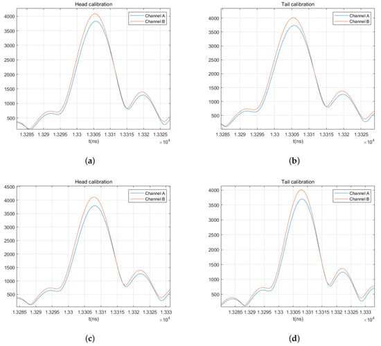
Figure 8.
After the dual-channel signal pulse compression of the internal calibration data, the peak position is partially enlarged. (a) The head calibration result of the first set of data; (b) the tail calibration result of the first set of data; (c) the head calibration result of the second of set data; (d) the tail calibration result of the second of set data.
Table 4.
The position offset of dual-channel images in range caused by each error.
Therefore, the position offset of the GF-3 ATI dual-channel image in range is mainly caused by the sampling time delay. At the same time, it also shows that the GF-3 ATI data are indeed the baseline errors that may be caused by antenna phase center position errors and attitude errors. Moreover, the range error between the dual channels caused by the baseline error is only on the order of millimeters.
3.1.2. Phase Imbalance Caused by Squint Imaging
According to Equation (19), the phase imbalance caused by the effect of squint imaging between Channel A and Channel B is formulated as:
The Doppler centroids estimated by the image of the two sets of GF-3 ATI data are shown in Figure 9, which is no longer zero and varies with the slant range. It can be found that the Doppler centroids of the two sets of GF-3 ATI data change by about 23 Hz and 20 Hz from near range to far range. Their change trend is basically consistent with that of the phase imbalances. Correspondingly, due to the existence of squint, the phase imbalances between channels changed by about 4.1 and 3.9 in range. Therefore, it is enough to show that the squint angle error exists in the imaging process of GF-3 ATI mode, and it is the main reason for the space-varying of the phase imbalance in range.
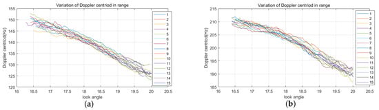
Figure 9.
The relative change of the Doppler centroid in range. (a) The first set of GF-3 ATI data; (b) the second set of GF-3 ATI data.
However, whether the squint imaging is caused by attitude control error or antenna electronic miss-pointing needs further discussion. The Doppler centroid frequency calculated from the attitude information is not consistent with the Doppler centroid frequency estimated by the GF-3 image. The Doppler centroids of the two sets of GF-3 ATI image data for phase imbalance error analysis are shown in Figure 10.
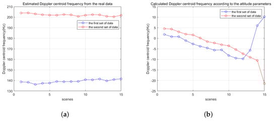
Figure 10.
The Doppler centroid frequency of the two sets of GF-3 ATI image data of the same channel. (a) The estimated Doppler centroid frequency from real data; (b) the calculated Doppler centroid frequency according to the attitude parameters.
The estimated Doppler centroid frequency difference between the two sets of data is about 60 Hz, and the Doppler change trend between different scenes is also different. Furthermore, the calculated Doppler centroid frequency difference between the two sets of data is much smaller than that of the estimated Doppler centroid frequency. Therefore, when the GF-3 attitude measurement results can truly reflect the actual attitude, we believe that the main reason for GF-3 squint imaging is the antenna electronic miss-pointing caused by the antenna thermal deformation. According to the Doppler centroid frequency of these two sets of data, the squint angle error can be calculated to be about 0.03 and 0.04, respectively. A Doppler centroid frequency error of 100 Hz will cause a radial velocity measurement error of 2.8 m/s. Therefore, to eliminate the dependence on the land scene, the calculated value of the Doppler centroid frequency from attitude measurements must be accurate enough for ocean current measurement. At the same time, it is necessary to ensure that the antenna electronic pointing is accurate enough for ocean current measurements.
3.1.3. Phase Imbalance Caused by the Baseline Error and the Phase Mismatch of the Antenna Pattern
After removing the phase imbalance caused by squint imaging, the main reasons for the remaining phase imbalances are the phase mismatch of the antenna pattern in range and the baseline errors caused by the antenna phase center position error and the attitude error. The remaining phase imbalances of the first set of data and the second set of data are shown in Figure 11, the accuracy of which depends on the accuracy of the estimated Doppler centroid frequency, satellite velocity, and effective baseline between channels. It can be found that the change of phase imbalance along the distance is less than 1, which basically meets the requirements of ocean current velocity measurement, and there is no consistent trend of the remaining phase imbalance between different scenes of the same set of data. In addition, only the attitude changes in the same imaging process of GF-3, and it can be concluded that GF-3 does have the baseline error caused by attitude error.
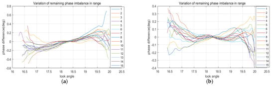
Figure 11.
The relative change of phase imbalances in range after removing the phase imbalance caused by squint imaging. (a) The first set of GF-3 ATI data; (b) the second set of GF-3 ATI data.
The baseline error caused by attitude error can be analyzed according to the GF-3 attitude information in echo data. We select the central scenes of two sets of data to analyze the attitude error. and represent the ideal pitch angle and yaw angle of satellite attitude, which are obtained by calculating the satellite orbit information using the 2D attitude steering approach for the zero Doppler centroid. and are the actual pitch and yaw angle measurements. The position errors of the dual-channel receiving position caused by the attitude error are shown in Table 5. For the first set of data, the pitch error is −0.0007, and the yaw error is 0.0018, corresponding to = −0.24 mm and = −0.09 mm. Similarly, for the second set of data, the pitch error is −0.0003, and the yaw error is 0.0025, corresponding to = −0.33 mm and = −0.04 mm. Moreover, the magnitude of baseline error can correspond to the magnitude of the position offset in the distance direction. On the premise of the accurate attitude measurement value, and the phase imbalance caused by the baseline error due to the attitude error can be expressed by Equation (19).
Table 5.
The attitude errors.
We carried out simulation experiments using the real radar parameters of the first set of GF-3 ATI data to analyze the phase imbalance caused by the deviation of the antenna phase center position causing the attitude error. The radar parameters used in the simulation are shown in Table 6. As shown in Figure 12, the phase imbalance between the two channels caused by the attitude error also has a near-linear change in the range, which is not a pure linear change. The phase imbalances caused by the attitude error of these two sets of data only changed by 0.0976 and 0.1242 from near range to far range, which is far less than the actual error. Therefore, on the premise that the attitude measurement is accurate enough, the baseline error caused by the satellite attitude error has little effect on the phase imbalance.
Table 6.
Simulated SAR parameters.
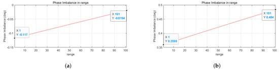
Figure 12.
The relative change of phase imbalances in range caused by the attitude error. (a) The first set of GF-3 ATI data; (b) the second set of GF-3 ATI data.
Moreover, there is no approximately linear change of the phase imbalance on both sides of the image, and the changing trend of the two sets of GF-3 ATI data with the same antenna beam is consistent. Therefore, it may be caused by the phase mismatch of the antenna pattern in range. However, the phase mismatch of the antenna pattern and the baseline error are coupled. Therefore, the phase imbalances caused by the antenna phase center position error and the phase mismatch of antenna pattern error cannot be distinguished. Therefore, it is necessary to calibrate the antenna pattern and antenna phase center position before the satellite is launched. This determines whether ATI-SAR can obtain accurate phase information and directly affects the ocean current inversion accuracy.
In conclusion, The causes of the space-varying of the phase imbalance are shown in Table 7, where and represent the antenna phase pattern in the range of Channel A and Channel B, respectively. It is considered that the space-varying of the phase imbalance in range of GF-3 ATI mode may be caused by the squint imaging, the baseline error, and the phase mismatch of the antenna pattern in range, according to these two sets of GF-3 ATI data. Moreover, squint imaging is the main factor causing phase imbalance in range caused by the attitude error and antenna electronic miss-pointing, while the baseline error and the phase mismatch of antenna pattern in range are minor factors. Finally, the block processing method mentioned in this paper can be used to calibrate the phase imbalance. In addition, under the condition of accurate attitude measurement, the main reason for the space-varying of phase imbalance in GF-3 ATI experimental mode is the antenna electronic miss-pointing. Of course, it is necessary to carry out the subsequent GF-3 ATI experiments to further study the phase imbalances of the GF-3 dual channels.
Table 7.
Causes of the space-varying of the phase imbalance in GF-3 ATI mode.
3.2. Ocean Current Measurements
On the one hand, due to the limited amount of data present, there is no sufficient reason to explain the source of phase imbalance between dual channels clearly. It is impossible to use a purely theoretical model to remove the influence of the phase imbalance. We can only use the phase imbalances of the sea-land junction scene data to subtract the corresponding land scene’s phase imbalances to extract the currents. On the other hand, the backscattered echo from the sea surface is mainly caused by Bragg scattering, when the radar incidence angle is between 20 and 60. Taking into account the above factors, we selected the following two scenes from the third set of GF-3 ATI data for phase imbalance calibration and current velocity measurement: the L1A-level product in the area near Qingdao, China, obtained by the GF-3 on 29 October 2019. The GF-3 images for current inversion are shown in Figure 13, and the product parameters are shown in Table 8. The wind field data are the ECMWF reanalysis data, with a time resolution of 1 h and a spatial resolution of 0.25× 0.25.
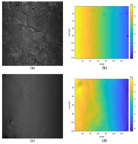
Figure 13.
The phase imbalances of the reference land scene and ocean scene for ocean current inversion. (a) The GF-3 image of the reference land scene; (b) the phase imbalances of the reference land scene; (c) the GF-3 image of the ocean scene; (d) the phase imbalances of the ocean scene.
Table 8.
Product parameters.
3.2.1. Current Measured by ATI Method
As shown in Figure 13, the phase imbalances of the reference land scene change obviously from near range to far range, which are about 9∼15, and that of the ocean scene also has a similar change in range. First of all, it is considered that in the same set of SAR data, the phase imbalance caused by satellite attitude, antenna miss-pointing, and antenna phase center position error in different scenes can be ignored. Therefore, the channel phase imbalances of this set of GF-3 data can be eliminated by estimating the phase imbalances of the land scene in the same set of data. The processing steps are shown in Figure 14.
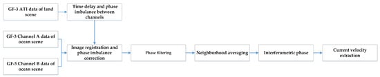
Figure 14.
GF-3 ATI data procession flow diagram.
Firstly, the time delay and phase imbalance between channels of the third set of GF-3 ATI data are calculated according to the steps shown in Figure 5 using the land scene data. Secondly, we perform image registration and phase imbalance calibration on the dual-channel data. Thirdly, we calculate the interferometric phase of the corresponding data. Furthermore, the obtained interferometric phase is processed by periodic pivoting filtering and averaged in the neighborhood to avoid noise, where the average window of the field is pixels, and the sliding step length of the azimuth and the range is 128 pixels. The spatial resolution is about 2 km × 2 km. Then, the phase imbalances of the ocean scene’s land area are set to zero to eliminate the phase imbalances between different scenes and the constant phase imbalances between the dual-channel system. The interferometric phases that can reflect the ocean surface motion are obtained. The radial velocities of the ocean surface are shown in Figure 15a. Finally, the empirical model mentioned in Section 2.1 is used to remove the contribution of ocean surface wind and the Bragg wave to ocean surface Doppler velocity, and the ocean current retrieved by the ATI method is shown in Figure 15b, which is about −145∼−30 cm/s.
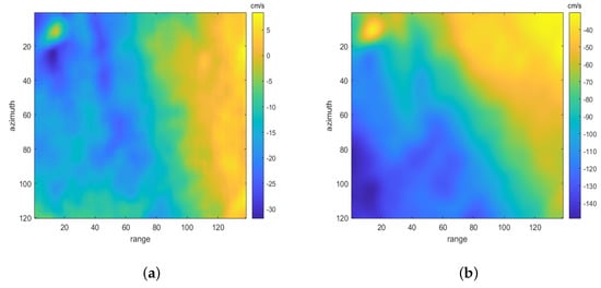
Figure 15.
The ocean current retrieved by the ATI method. (a) The radial velocities of the ocean surface; (b) the ocean current velocities.
3.2.2. Verification of Inversion Accuracy
In order to verify the accuracy of the ocean surface radial velocity extracted from GF-3 ATI data, mutual verification has to be carried out with the currents obtained by the DCA method using single-channel data. The Doppler centroid frequency calculated from the SAR signal of the ocean is caused by the motion of the stationary target relative to the satellite and the ocean surface motion [33]. The Doppler centroid frequency estimated from the SAR echo data can be expressed as:
where is the Doppler shift caused by the motion of the ocean surface and is the Doppler frequency shift caused by the satellite orbit, attitude, antenna electronic miss-pointing, and the rotation of the Earth. Generally speaking, is zero for land scenes since GF-3 uses the 2D attitude steering approach for the zero Doppler centroid. Based on this feature, we can also use the land scene as a reference scene to eliminate the component in the Doppler centroid frequency of the ocean scene. The estimated Doppler centroid frequency can be calculated by the correlation Doppler estimator (CDE) method [34].
For the DCA method, we also use the land scene as a reference scene to eliminate the component, which is caused by the satellite orbit, satellite attitude, antenna electronic pointing, and the rotation of the Earth in the Doppler centroid frequency of the ocean scene. The way to extract the velocities of the ocean current from the Doppler velocities of the ocean surface is exactly the same as the ATI method. The result is shown in Figure 16. The ocean current retrieved by the DCA method is about −140∼−30 cm/s.
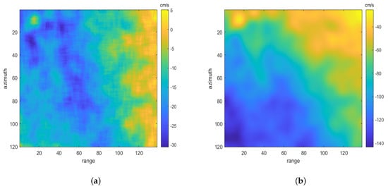
Figure 16.
The results retrieved by the Doppler centroid analysis (DCA) method. (a) The radial velocities of the ocean surface; (b) the ocean current velocities.
The mean difference between the current velocities obtained by the ATI method and the DCA method is −0.010 m/s, and the root mean squared error (RMSE) is 0.062 m/s. The correlation coefficient reaches 0.98. As shown in Figure 17, the difference of the current velocities obtained by the two methods is mainly −0.05 m/s ∼0.05 m/s. Therefore, it can be proven that the accuracy of ocean current retrieval by ATI-SAR with a short baseline is basically the same as that of the DCA method based on single-channel SAR data.
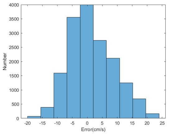
Figure 17.
Statistical chart of the error distribution of the ocean current obtained by the two methods.
Finally, the accuracy of the inversion results is verified with the current velocities measured by high-frequency surface wave radar (HFSWR). First of all, the ocean currents measured by HFSWR are matched with those retrieved by GF-3 ATI data by bilinear interpolation. Comparing the current velocities measured by GF-3 ATI data and HFSWR, the RMSE is 0.38 m/s, the mean difference being −0.33 m/s, and the correlation coefficient reaching 0.62, which preliminarily verify the correctness of the analysis of this paper. In addition, the ocean current inversion method based on GF-3 ATI data and its accuracy improvement still need to be further studied.
4. Discussion
In this paper, we firstly introduce and analyze the basic ocean current measurement principles by ATI mode. We deduce and analyze the theoretical formula of the cause of phase imbalance and then locate the source of the phase imbalance of GF-3 ATI mode using real data. Finally, according to the phase imbalance of the land scene in the same set of data, the phase imbalance of the ocean scene is calibrated, and the current velocity is measured. The current measured by the DCA method and HFSWR is used to verify the results measured by the ATI method. The contributions to the RMSE and the mean difference between the current measured by the ATI method and HFSWR are expected in many aspects. First of all, the phase imbalance error of the land scene cannot truly reflect the phase imbalance of the ocean scene. There is a time-varying phase imbalance in the azimuth due to satellite attitude and satellite velocity, which is not considered in the process of eliminating the phase imbalance between channels. Therefore, the calculated ocean surface radial velocity may not accurately reflect the Doppler velocity caused by ocean surface motion. Secondly, the accuracy of the retrieved current highly depends on the empirical model we used. For example, the CDOP model is obtained by using a three-layer neural network training the Doppler frequency shift of ASAR data and the wind retrieved by ASCAT; whether it is suitable for GF-3 data needs further verification. Thirdly, the accuracy of sea surface current velocity is sensitive to wind speed and wind direction error. However, the spatial resolution of ECMWF reanalysis data is lower than that of the GF-3 image, and they cannot match completely in time. In addition, the results also depend on the accuracy of current velocities measured by HFSWR. Therefore, it is hoped that we can obtain the in situ sea surface wind data and current velocity data to more accurately prove the accuracy of GF-3 data in ocean current inversion.
According to our analysis of GF-3 ATI data, the current velocity measured by the ATI method based on dual channel data is basically consistent with that measured by the DCA method based on single-channel data. Furthermore, the ATI method needs dual receiving antennas or antenna arrays, while the DCA method only needs a single antenna, which is much simpler than the ATI method in hardware. Almost all SAR satellites have the ability of the DCA method for current measurement, which is more conducive to the operational measurement of current velocity. However, GF-3 ATI mode only has a 3.75 m along-track interferometric baseline, which is a short baseline. It can only show that the ATI method and DCA method have the same current measurement accuracy in the case of a short baseline. In addition, according to Romeiser’s research on TerraSAR-X data [11], the short-baseline ATI method and DCA method have the same accuracy in general, but the short-baseline ATI method has certain advantages compared with the DCA method in river measurement and ocean internal wave measurement. In addition, the ATI method can be used to measure the current velocity with high spatial resolution, which is much higher than the DCA method. In theory, the spatial resolution of the ATI method is consistent with that of SAR imaging; to improve the inversion accuracy, spatial average processing is needed, which reduces the spatial resolution of the current measurement by the ATI method. However, in order to obtain high-precision Doppler centroid frequency, the DCA method must carry out large-scale spatial averaging. In other words, the spatial resolution of the ATI method with a long along-track interferometric baseline is higher than that of the DCA method with the same accuracy.
Due to the influence of image saturation distortion and different antenna beams, we can only rely on these two sets of existing data to get corresponding conclusions. On the one hand, the attitude control error, attitude measurement error, and antenna electronic miss-pointing of GF-3 need further analysis. Therefore, we look forward to arranging special GF-3 missions in the future and obtaining corresponding dual channel antenna patterns to better verify and find out the reasons for the phase imbalance of GF-3 ATI mode. The following data are expected to be obtained, such as ATI data of the land scene with the same scanning angle and different observation directions, preferably GF-3 ATI data of tropical rainforests and the equatorial region. On the other hand, the ocean current measured by the GF-3 ATI data must rely on the land scene to eliminate the phase imbalances due to GF-3 dual channel phase imbalance. Therefore, accurate modeling and analysis of channel phase imbalance are needed to get rid of the dependence on the land scene in the subsequent research. Moreover, how to accurately eliminate the contribution of sea surface wind and Bragg phase velocity to Doppler velocity is also an essential research content.
5. Conclusions
GF-3 ATI mode performs imaging through dual-receive fine stripmap mode, which has an effective along-track antenna separation of 3.75 m. Using the ATI method to invert the current requires the high precision of the interferometric phase. Simply subtracting the constant phase imbalance between the two channels is not sufficient for measurement accuracy. The space-time variability of the phase imbalance between channels, caused by antenna phase center position error, attitude error, antenna electronic miss-pointing, antenna pattern mismatch, and other reasons, cannot be ignored. This paper introduces a phase imbalance calibration method based on SAR data. Using the characteristic that the phase difference of two channels changes linearly with the Doppler frequency in the Doppler frequency domain, the signal delay and phase imbalance between channels are calculated by the least squares method. The advantage of this method is that it can carry out dual channel image registration and target radial velocity measurement when the along-track interferometric baseline and satellite velocity are unknown, and the influence of the along-track interferometric baseline error and the satellite velocity measurement error can be ignored. Finally, the space-time change of the phase imbalance is solved by image block processing.
Limited by the number of GF-3 ATI data, we mainly analyzed the phase imbalance in range of two sets of GF-3 ATI data with the same antenna beam combined with the simulation experiment using actual GF-3 parameters. It was concluded that the phase imbalance in the range of GF-3 ATI mode is mainly caused by squint imaging, the baseline error, and the phase mismatch of the antenna pattern in range. Furthermore, the space-varying of the phase imbalance caused by the baseline error and the phase mismatch of the antenna pattern in range is far less than that caused by squint imaging, which is mainly caused by satellite attitude error and antenna electronic miss-pointing. What is more, on the premise of accurate attitude measurement results, the influence of the GF-3 attitude control error on the phase imbalance can be ignored, and the main reason for the space-varying of phase imbalance in GF-3 ATI experimental mode is the antenna electronic miss-pointing.
After the phase imbalances’ calibration, we carried out the ocean current by the ATI method and the DCA method. The results obtained by the two methods are relatively consistent with the correlation coefficient of 0.98. The mean difference is −0.010 m/s, and the RMSE is 0.062 m/s. Compared with the current measured by HFSWR, the RMSE is around 0.38 m/s. Therefore, it illustrates the feasibility of using GF-3 data to measure ocean currents, whether dual-channel or single-channel data. It can be proven that the accuracy of ocean current inversion through the short-baseline ATI-SAR is basically the same as that of the DCA method based on single-channel SAR data.
Author Contributions
Conceptualization, J.Y. and X.Y.; Data curation, J.Y., X.Y. and L.Z.; Formal analysis, J.Y.; Funding acquisition, B.H.; Investigation, J.Y. and J.S.; Methodology, J.Y., X.Y. and B.H.; Project administration, B.H.; Resources, L.Z.; Software, J.Y.; Supervision, C.D.; Validation, J.Y., J.S. and M.S.; Visualization, J.Y.; Writing—original draft, J.Y.; Writing—review & editing, J.Y., X.Y., B.H., M.S. and X.W. All authors have read and agreed to the published version of the manuscript.
Funding
This research was funded by the National Natural Science Foundation of China under Grant Number 41976169.
Conflicts of Interest
The authors declare no conflict of interest.
References
- Goldstein, R.M.; Zebker, H.A. Interferometric radar measurement of ocean surface currents. Nature 1987, 328, 707–709. [Google Scholar] [CrossRef]
- Goldstein, R.M.; Zebker, H.A.; Barnett, T.P. Remote sensing of ocean currents. Science 1989, 246, 1282–1285. [Google Scholar] [CrossRef] [PubMed]
- Moller, D.; Frasier, S.J.; Porter, D.L.; McIntosh, R.E. Radar-derived interferometric surface currents and their relationship to subsurface current structure. J. Geophys. Res. Oceans 1998, 103, 12839–12852. [Google Scholar] [CrossRef]
- Romeiser, R.; Thompson, D.R. Numerical study on the along-track interferometric radar imaging mechanism of oceanic surface currents. IEEE Trans. Geosci. Remote Sens. 2000, 38, 446–485. [Google Scholar] [CrossRef]
- Kim, D.J.; Moon, W.M.; Moller, D.; Imel, D.A. Measurements of ocean surface waves and currents using L-and C-band along-track interferometric SAR. IEEE Trans. Geosci. Remote Sens. 2003, 41, 2821–2832. [Google Scholar]
- Romeiser, R.; Breit, H.; Eineder, M.; Runge, H.; Flament, P.; De Jong, K.; Vogelzang, J. Current measurements by SAR along-track interferometry from a space shuttle. IEEE Trans. Geosci. Remote Sens. 2005, 43, 2315–2324. [Google Scholar] [CrossRef]
- Romeiser, R.; Suchandt, S.; Runge, H.; Steinbrecher, U.; Grunler, S. First analysis of TerraSAR-X along-track InSAR-derived current field. IEEE Trans. Geosci. Remote Sens. 2010, 48, 820–829. [Google Scholar] [CrossRef]
- Chapron, B.; Collard, F.; Ardhuin, F. Direct measurement of ocean surface velocity from space: Interpretation and validation. J. Geophys. Res. Oceans 2005, 110, C07008. [Google Scholar] [CrossRef]
- Rouault, M.J.; Mouche, A.; Collard, F.; Johannessen, J.A.; Chapron, B. Mapping the aguhas current from space: An assessment of ASAR surface current velocity. J. Geophys. Res. Oceans 2010, 115, C10026. [Google Scholar] [CrossRef]
- Hansen, M.W.; Collard, F.; Dagestad, K.F.; Johannessen, J.A.; Chapron, B. Retrieval of sea surface range velocity from envisat ASAR Doppler centroid measurements. IEEE Trans. Geosci. Remote Sens. 2011, 49, 3582–3592. [Google Scholar] [CrossRef]
- Romeiser, R.; Runge, H.; Suchandt, S.; Kahle, R.; Rossi, C.; Bell, P.S. Quality Assessment of Surface Current Fields From TerraSAR-X and TanDEM-X Along-Track Interferometry and Doppler Centroid Analysis. IEEE Trans. Geosci. Remote Sens. 2013, 52, 2759–2772. [Google Scholar] [CrossRef]
- Han, B.; Ding, C.B.; Zhong, L.H.; Liu, J.Y.; Qiu, X.L.; Hu, Y.X.; Lei, B. The GF-3 SAR data processor. Sensors 2018, 18, 835. [Google Scholar] [CrossRef] [PubMed]
- Shang, M.Y.; Qiu, X.L.; Han, B.; Yang, J.Y.; Zhong, L.H.; Ding, C.B.; Hu, Y.X. The Space-Time Variation of Phase Imbalance for GF-3 Azimuth Multichannel Mode. IEEE J. Sel. Top. Appl. Earth Obs. Remote Sens. 2020, 13, 4774–4788. [Google Scholar] [CrossRef]
- Shang, M.Y.; Qiu, X.L.; Han, B.; Ding, C.B.; Hu, Y.X. Channel imbalances and along-track baseline estimation for the GF-3 azimuth multichannel mode. Remote Sens. 2019, 11, 1297. [Google Scholar] [CrossRef]
- Krieger, G.; Gebert, N.; Moreira, A. Unambiguous SAR signal reconstruction from nonuniform displaced phase center sampling. IEEE Geosci. Remote Sens. Lett. 2005, 1, 260–264. [Google Scholar] [CrossRef]
- Gebert, N.; Krieger, G.; Moreira, A. Digital beamforming on receive: Techniques and optimization strategies for high-resolution wide-swath SAR imaging. IEEE Trans. Aerosp. Electron. Syst. 2009, 45, 564–592. [Google Scholar] [CrossRef]
- Ding, C.B.; Jin, T.T.; Qiu, X.L.; Hu, D.H. Velocity estimation of moving targets for spaceborne multichannel synthetic aperture radar systems based on equivalent along-track interferometry technique. IET Radar Sonar Navig. 2018, 12, 964–972. [Google Scholar] [CrossRef]
- López-Dekker, P.; De Zan, F.; Wollstadt, S.; Younis, M.; Danielson, R.; Tesmer, V.; Martins Camelo, L. A ku-Band ATI SAR Mission for Total Ocean Surface Current Vector Retrieval: System Concept and Performance. In Proceedings of the ESA Advanced RF Sensors and Remote Sensing Instruments (ARSI) and Ka-Band Earth Observation Radar Missions (KEO), Noordwijk, The Netherlands, 4–7 November 2014; pp. 1–8. [Google Scholar]
- Imel, D.D.A.; Hensley, S.; Pollard, B.; Chapin, E.; Rodriguez, E. AIRSAR Along-Track Interferometry. AIRSAR Earth Science and Applications Workshop. 2002; pp. 1–58. Available online: https://airsar.jpl.nasa.gov/news/atiPaper.pdf (accessed on 24 December 2020).
- Song, X.; Wang, J.; Chu, X. Estimation of sea surface velocities from sar images using the Doppler shift. Remote Sens. Technol. Appl. 2019, 34, 293–302. [Google Scholar]
- Mouche, A.A.; Collard, F.; Chapron, B.; Dagestad, K.F.; Guitton, G.; Johannessen, J.A.; Kerbaol, V.; Hansen, M.W. On the use of Doppler shift for sea surface wind retrieval from SAR. IEEE Trans. Geosci. Remote Sens. 2012, 50, 2901–2909. [Google Scholar] [CrossRef]
- Elyouncha, A.; Eriksson, L.E.B.; Romeiser, R.; Ulander, L.M.H. Phase calibration of TanDEM-X ATI-SAR data for sea surface velocity measurements. In Proceedings of the 2017 IEEE Geoscience and Remote Sensing Symposium (IGARSS 2017), Fort Worth, TX, USA, 23–28 July 2017; pp. 922–925. [Google Scholar]
- Feng, J.; Gao, C.; Zhang, Y.; Wang, R. Phase mismatch calibration of the multichannel SAR based on azimuth cross correlation. IEEE Geosci. Remote Sens. Lett. 2012, 10, 903–907. [Google Scholar] [CrossRef]
- Zhang, S.X.; Xing, M.D.; Xia, X.G.; Zhang, L.; Guo, R.; Liao, Y.; Bao, Z. Multichannel HRWS SAR imaging based on range-variant channel calibration and multi-Doppler-direction restriction ambiguity suppression. IEEE Trans. Geosci. Remote Sens. 2013, 52, 4306–4327. [Google Scholar] [CrossRef]
- Zhang, L.; Xing, M.D.; Qiu, C.W.; Bao, Z. Adaptive two-step calibration for high-resolution and wide-swath SAR imaging. IET Radar Sonar Navig. 2010, 4, 548–559. [Google Scholar] [CrossRef]
- Yang, T.; Li, Z.; Liu, Y.; Bao, Z. Channel error estimation methods for multichannel SAR systems in azimuth. IEEE Geosci. Remote Sens. Lett. 2012, 10, 548–552. [Google Scholar] [CrossRef]
- Toporkov, J.V.; Hwang, P.A.; Sletten, M.A.; Farquharson, G.; Perkovic, D.; Frasier, S.J. Surface velocity profiles in a vessel’s turbulent wake observed by a dual-beam along-track interferometric SAR. IEEE Geosci. Remote Sens. Lett. 2011, 8, 602–606. [Google Scholar] [CrossRef]
- Farquharson, G.; Deng, H.; Goncharenko, Y.; Mower, J. Dual-beam ATI SAR measurements of surface currents in the nearshore ocean. In Proceedings of the 2014 IEEE Geoscience and Remote Sensing Symposium (IGARSS 2014), Quebec City, QC, Canada, 13–18 July 2014; pp. 2661–2664. [Google Scholar]
- Mancon, S.; Guarnieri, A.M.; Giudici, D.; Tebaldini, S. On the phase calibration by multisquint analysis in TOPSAR and stripmap interferometry. IEEE Trans. Geosci. Remote Sens. 2016, 55, 134–147. [Google Scholar] [CrossRef]
- López-Dekker, P.; Schaefer, C.; Tienda, C.; Younis, M.; Ludwig, M. Ka-Band SAR Instrument with Joint XTI-ATI Mode Capability. In Proceedings of the 19th Ka and Broadband Communiations, Navigation and Earth Observation Conference, Florence, Italy, 14–17 October 2013; pp. 14–17. [Google Scholar]
- Gabriel, A.K.; Goldstein, R.M. Crossed orbit interferometry: Theory and experimental results from SIR-B. Int. J. Remote Sens. 1988, 9, 857–872. [Google Scholar] [CrossRef]
- Cheng, S.; Zhang, Z.Y.; Shi, W.P. Precise coregistration for complex images based on precise satellite orbit data. Eng. Surv. Mapp. 2010, 2, 6–8. [Google Scholar]
- He, Y.J.; Liu, B.C.; Zhang, B.; Cheng, Z.B.; Qiu, Z.F. Overview on Satellite Remote-sensing Methods for Sea-surface-current Measurement. Guangxi Sci. 2015, 22, 294–300. [Google Scholar]
- Madsen, S.N. Estimating the Doppler centroid of SAR data. IEEE Trans. Aerosp. Electron. Syst. 1989, 25, 134–140. [Google Scholar] [CrossRef]


Publisher’s Note: MDPI stays neutral with regard to jurisdictional claims in published maps and institutional affiliations. |
© 2021 by the authors. Licensee MDPI, Basel, Switzerland. This article is an open access article distributed under the terms and conditions of the Creative Commons Attribution (CC BY) license (http://creativecommons.org/licenses/by/4.0/).