Leveraging TLS as a Calibration and Validation Tool for MLS and ULS Mapping of Savanna Structure and Biomass at Landscape-Scales

Abstract

Savanna ecosystems are challenging to map and monitor as their vegetation is highly dynamic in space and time. Understanding the structural diversity and biomass distribution of savanna vegetation requires high-resolution measurements over large areas and at regular time intervals. These requirements cannot currently be met through field-based inventories nor spaceborne satellite remote sensing alone. UAV-based remote sensing offers potential as an intermediate scaling tool, providing acquisition flexibility and cost-effectiveness. Yet despite the increased availability of lightweight LiDAR payloads, the suitability of UAV-based LiDAR for mapping and monitoring savanna 3D vegetation structure is not well established. We mapped a 1 ha savanna plot with terrestrial-, mobile- and UAV-based laser scanning (TLS, MLS, and ULS), in conjunction with a traditional field-based inventory (n = 572 stems > 0.03 m). We treated the TLS dataset as the gold standard against which we evaluated the degree of complementarity and divergence of structural metrics from MLS and ULS. Sensitivity analysis showed that MLS and ULS canopy height models (CHMs) did not differ significantly from TLS-derived models at spatial resolutions greater than 2 m and 4 m respectively. Statistical comparison of the resulting point clouds showed minor over- and under-estimation of woody canopy cover by MLS and ULS, respectively. Individual stem locations and DBH measurements from the field inventory were well replicated by the TLS survey (R${}^2$ = 0.89, RMSE = 0.024 m), which estimated above-ground woody biomass to be 7% greater than field-inventory estimates (44.21 Mg ha${}^{-1}$ vs 41.08 Mg ha${}^{-1}$). Stem DBH could not be reliably estimated directly from the MLS or ULS, nor indirectly through allometric scaling with crown attributes (R${}^2$ = 0.36, RMSE = 0.075 m). MLS and ULS show strong potential for providing rapid and larger area capture of savanna vegetation structure at resolutions suitable for many ecological investigations; however, our results underscore the necessity of nesting TLS sampling within these surveys to quantify uncertainty. Complementing large area MLS and ULS surveys with TLS sampling will expand our options for the calibration and validation of multiple spaceborne LiDAR, SAR, and optical missions.

1. Introduction

Savanna vegetation structure is shaped by the interaction of climate, soils and a variety of disturbance agents acting at multiple spatio-temporal scales [1,2]. The actions of fire, herbivores, termites, and cyclones have marked effects on the structure of savanna tree crowns, leading to high degree of structural diversity [3,4,5]. Mapping and monitoring the structure of savanna ecosystems is therefore challenging not only because of their heterogeneous spatial patterning, but also because of disturbance driven variability in individual tree crown structure [6]. Structural attributes such as height, canopy diameter, and projected foliage cover are commonly assessed through field inventories—but these measures are often subjective and prone to sampling errors [7]. Robust assessment of structural change in tropical savannas requires methods that can account for spatial and temporal heterogeneity, and a high level of accuracy and precision in structural attribute measurement.

Remote sensing is very attractive from a monitoring and management perspective, offering large area assessment at ever increasing spatial, temporal and spectral resolutions [8,9]. Despite many advances in spaceborne imaging technology, savanna ecosystems remain challenging from an earth observation perspective due to their inherent mix of discontinuous woody cover and herbaceous vegetation [10]. Light-detection-and-ranging (LiDAR), especially airborne laser scanning (ALS), has emerged as a prominent technology for mapping and monitoring vegetation in a variety of ecosystems across the globe [11]. ALS is particularly well suited to the measurement of savanna ecosystem structure where it can delineate subtle topographic and vegetation characteristics [12]. The inclusion of ALS in ecological studies has advanced the field of savanna ecology, revealing new insights into the controls and drivers of carbon storage [13,14], and providing pathways for understanding how vegetation structure influences the ecology and diversity of various fauna [15,16].

Nonetheless, despite the many advantages of ALS, certain ecological processes operate at even finer spatial scales than can be assessed from traditional airborne platforms. Detecting stress, sub-canopy structural changes, and recruitment dynamics are all examples of processes that sit at the limits of airborne surveying. Terrestrial laser scanning (TLS) has emerged as the gold standard for fine-scale 3D reconstruction of above-ground elements, and is increasingly being used in forestry and ecological surveying [17,18]. One of the main constraints of TLS is the time-intensive nature of data acquisition and post-processing, and the relatively small spatial extent that can feasibly be covered [19]. Newer sensors are overcoming some of these barriers by increasing the speed and ranging distance, and enabling larger area coverage in suitable environmental conditions [20]. Reduced size and weight of modern LiDAR sensors has broadened the field of UAV-based laser scanning (ULS), offering a high degree of acquisition flexibility and increased spatial resolution due to lower and slower flying speeds [21,22,23]. In conjunction with these developments, handheld and mobile laser scanning (MLS) systems have also been gaining traction, enabling greater freedom of movement and increased speed of acquisition in comparison to TLS. MLS enables navigation in confined spaces, and the continuous mapping approach can reduce occlusion and provide thorough coverage in complex environments [24,25,26].

Given these recent advances in LiDAR sensor and platform technologies, choosing the right solution for a particular mapping and monitoring problem has become more challenging. The relative strengths and weaknesses of different systems needs to be explored across a range of ecosystems to best match system performance with the specific research or management objectives. The objective of this study was to assess the degree of divergence and complementarity of three different laser scanning systems for capturing the 3D structure of tropical savanna woodland structure. We explore the relative strengths and weaknesses of terrestrial laser scanning (TLS), mobile laser scanning (MLS) and UAV laser scanning (ULS) in a vegetation monitoring context, by addressing two key questions:

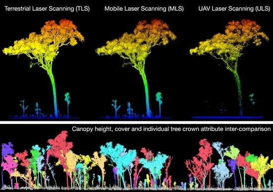
• Are there significant differences in the representation of woody canopy height and cover captured by TLS, MLS and ULS?
• How reliably can tree stem DBH and above-ground woody biomass be mapped from TLS, MLS and ULS?

2. Materials and Methods

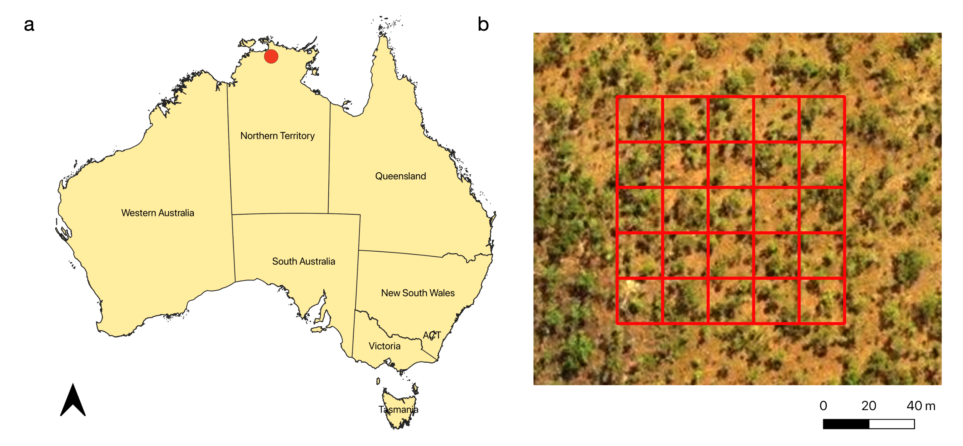
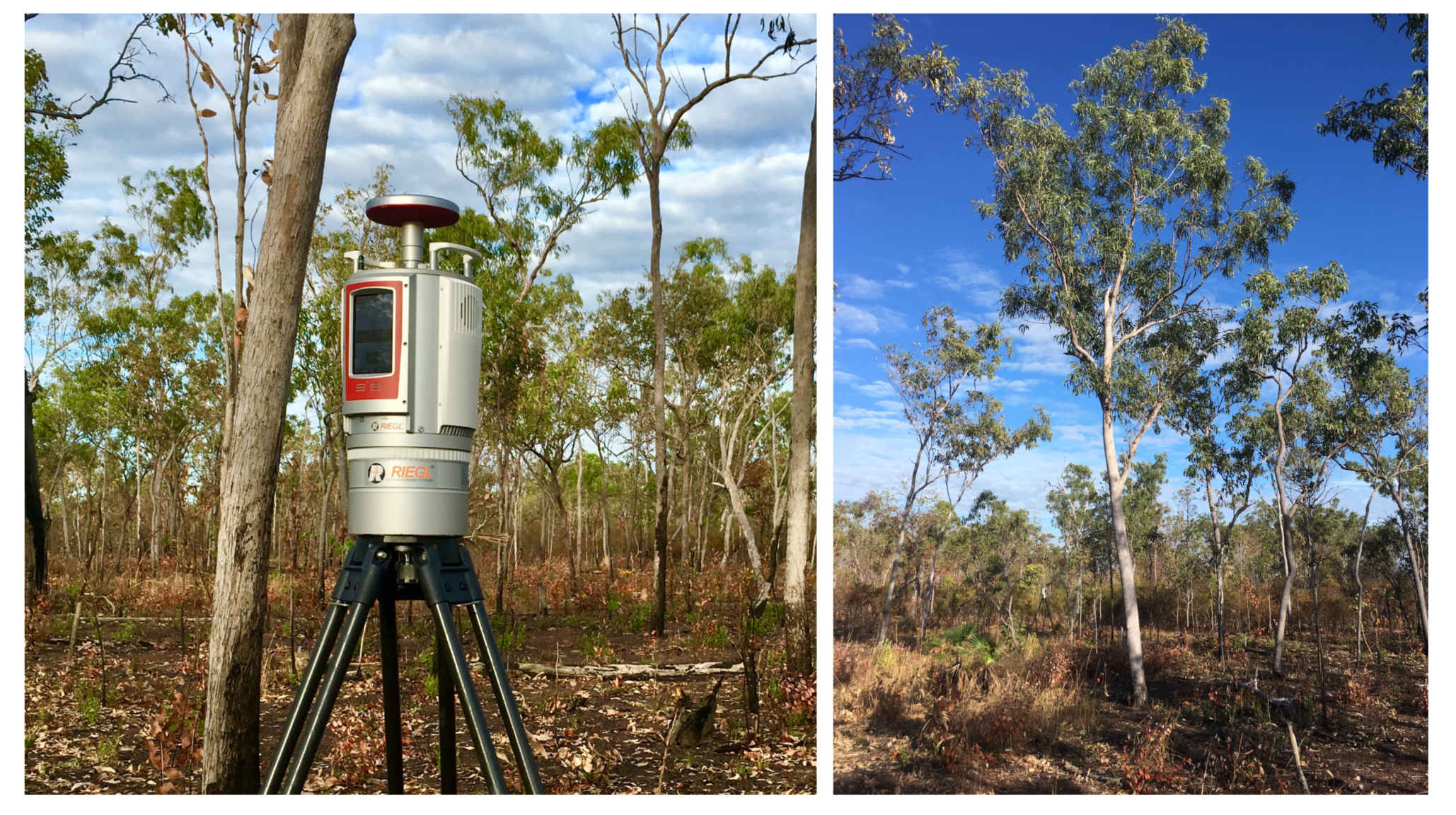
2.1. Study Site

This study was undertaken in northern Kakadu National Park in the Northern Territory of Australia (Figure 1). The climate is tropical, with maximum and minimum temperature averaging 34.1${}^{\circ }$C and 22.6 ${}^{\circ }$C respectively (Köppen climate classification = Aw). Rainfall is highly seasonal, with the vast majority of the annual 1557 mm yr${}^{-1}$ falling predominantly in the December—March wet season [27]. The vegetation is representative of much of the Australian tropical savanna zone, with an over-storey dominated by Eucalyptus tetrodonta, Eucalyptus miniata, and Erythrophleum chlorostachys. The under-storey is characterized by annual grasses, particularly Sorghum species. Our data collection campaign took place on 23/24 July 2019, well into the dry season and one month after a fire passed through—the occurrence of which is typical every 1–2 years in this system [28]. The herbaceous grass layer was reduced by the fire, but small shrubs were still present.

2.2. Field Inventory

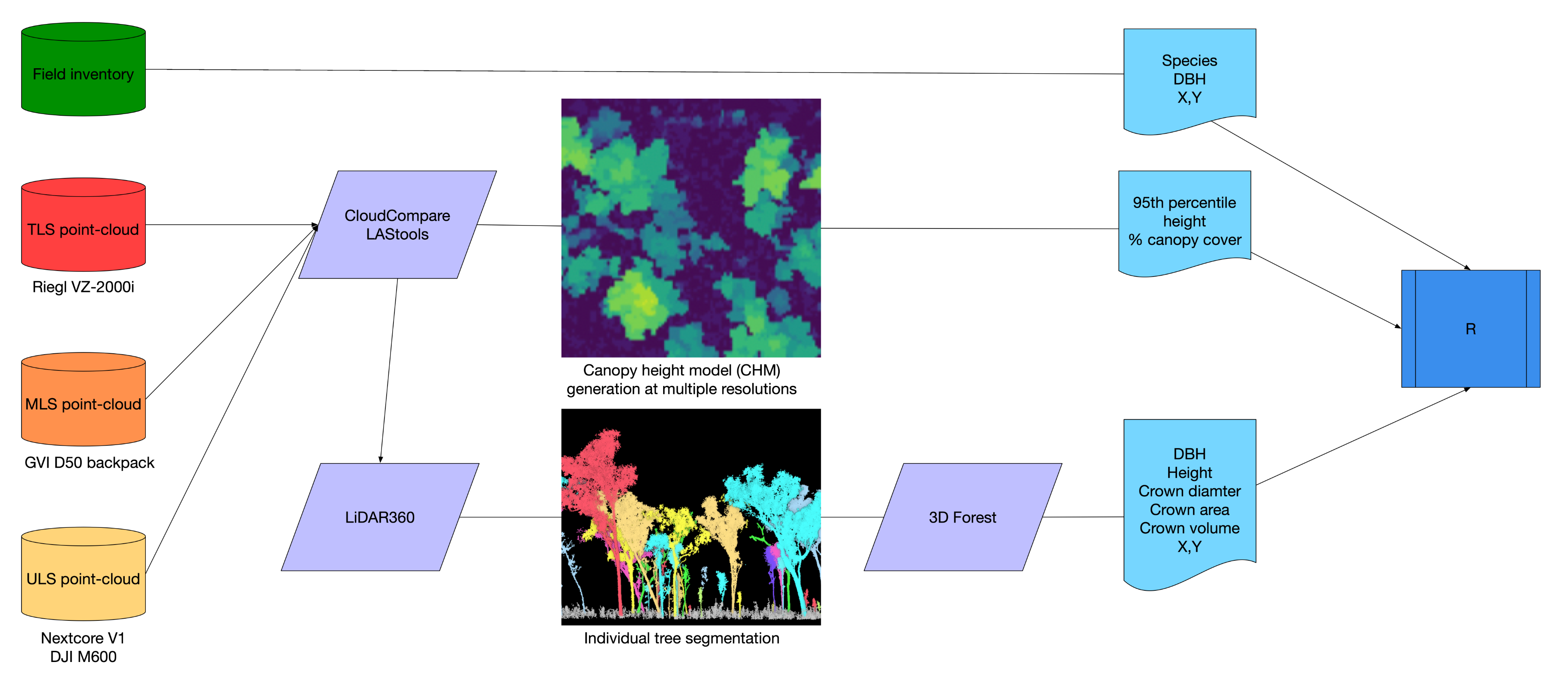
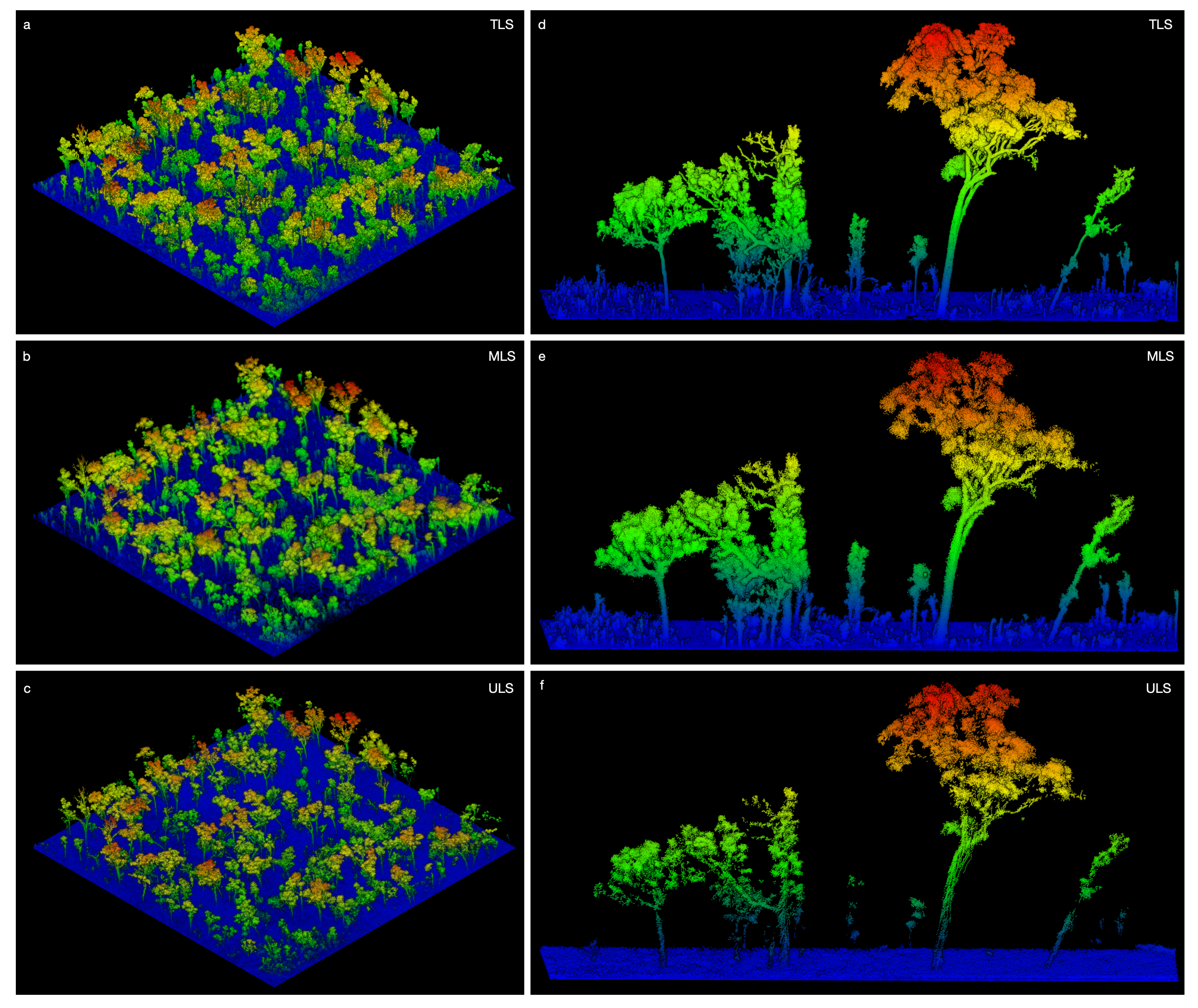
A series of long-term monitoring plots were established in the savanna woodlands of the Jabiru region in 2017 to provide reference sites for understanding natural system dynamics and informing the closure criteria of the adjacent Ranger uranium mine [29]. Each plot measures 100 m × 100 m, and the four corners and center are marked with permanent posts. We selected one of these sites for our study and each woody plant with a stem diameter > 0.03 m and that was > 1.5 m in height was inventoried in the field. Survey tapes were laid out in a 20 m × 20 m grid to guide the field crew, and each individual tree was: (i) tagged with a RTK dGPS (Leica GS16 with Precise Point Positioning); (ii) identified to species level; and (iii) measured with a DBH tape at 1.3 m above ground level. A total of 521 trees consisting of 572 stems were inventoried in the field.

2.3. Laser Scanning

The selected site was surveyed on 24 July 2019 with three different LiDAR systems, operating from terrestrial, mobile and UAV platforms (

Table 1. Instrument, surveying, and processing characteristics of the three LiDAR systems. Reported point densities are after the application of a 0.01 m sub-sampling spatial filter. Note: TLS = terrestrial laser scanning, MLS = mobile laser scanning, ULS = UAV laser scanning.

	TLS	MLS	ULS
Instrument	Riegl VZ-2000i	LiBackPack D50	Nextcore Version 1
Manufacturer	Riegl	Green Valley International	Nextcore
Sensor	Riegl	Velodyne	Quanergy M8
Platform	Tripod	Backpack	Drone (DJI M600)
Acquisition time	120 min	20 min	15 min
Co-registration processing time	60 min	20 min	20 min
Filtered point density (m${}^2$)	7340	2401	2015

). Terrestrial laser scanning (TLS) was conducted from a surveying tripod at 1.8 m agl, using a Riegl VZ-2000i system with integrated RTK-GNSS (Figure 2). Sixteen scan locations were established, using a regular grid spacing of 30 m. The scanner was operated at 600 kHz with an angular sampling resolution of 30 mdeg. The scanner communicated with a RTK base station (Emlid RS2) established at the site and operating over a LoRa network. Real-time positioning error of the scanner at each scan location was < 0.05 m.

Mobile laser scanning (MLS) was conducted with a GreenValley LiBackpack D50. The unit consists of two Velodyne VLP-16 sensors, one operating vertically and one horizontally. The system uses Simultaneous Location and Mapping (SLAM) technology for co-registration. The MLS system was carried as a backpack by a field technician who walked slowly through the site ensuring consistent coverage and loop closure. The trajectory of the mobile unit was displayed in real time to the operator via a tablet to ensure full coverage of the site.

UAV laser scanning (ULS) point clouds were collected using the Nextcore® system (www.nextcore.co) which uses a Quanergy M8 discrete return LiDAR sensor integrated with a Spatial Dual (www.advancednavigation.com) INS including IMU and dual antenna RTK GPS, mounted on a DJI Matrice 600 Pro. The UAV was flown in a grid pattern at 3.5 ms${}^{-1}$ at approximately 40 m agl with a line spacing of 18 m. The sensor pulse rate was 1200 kHz, which resulted in average point densities of 2000 points per m${}^2$ within the one hectare plot.

2.4. Point-Cloud Processing

Raw processing of the TLS dataset was conducted in Riegl’s RiSCAN Pro software suite (v2.9). Scan data were projected into the WGS84 coordinate system (UTM Zone 53S) and filtered for noise based on reflectance and deviation characteristics. The Multi-Station Adjustment (MSA) plugin was used to finely co-register the individual scans, which were already well positioned given the integrated GNSS with real-time correction.

Raw MLS data were converted to a point cloud incorporating the IMU data from the backpack using proprietary SLAM algorithms in the LiBackpack software from GreenValley International. The point cloud was geo-referenced in LiDAR360 by detecting six pyramid structures that were placed throughout the site as ground controls. The 3D RTK-GNSS location of the peaks of each pyramid were recorded during the field campaign.

ULS point clouds were PPK geo-registered using the proprietary Nextcore® software. Each of the flight-lines underwent a statistical outlier removal (SOR) filter in CloudCompare. The number of neighbors used to compute mean distance was set to 10, and the standard deviation multiplier was set to 2. There was still some systematic misalignment of flight-lines following the PPK correction. To correct for this, each flight-line was sequentially registered to its neighbor using the Iterative Closest Point (ICP) algorithm implemented in CloudCompare. The random sample limit was set to 250,000 and RMS error difference threshold set to $1 \times {10}^{-08}$. After registration, flight-line point clouds were merged into a single point cloud.

Co-registered point clouds from each platform were exported to the ASPRS LAS format version 1.4 for further analysis. A 0.01 m spacing filter was applied to all three clouds to remove duplicate points and ensure an even distribution of points across the landscape.

2.5. Structural Analysis

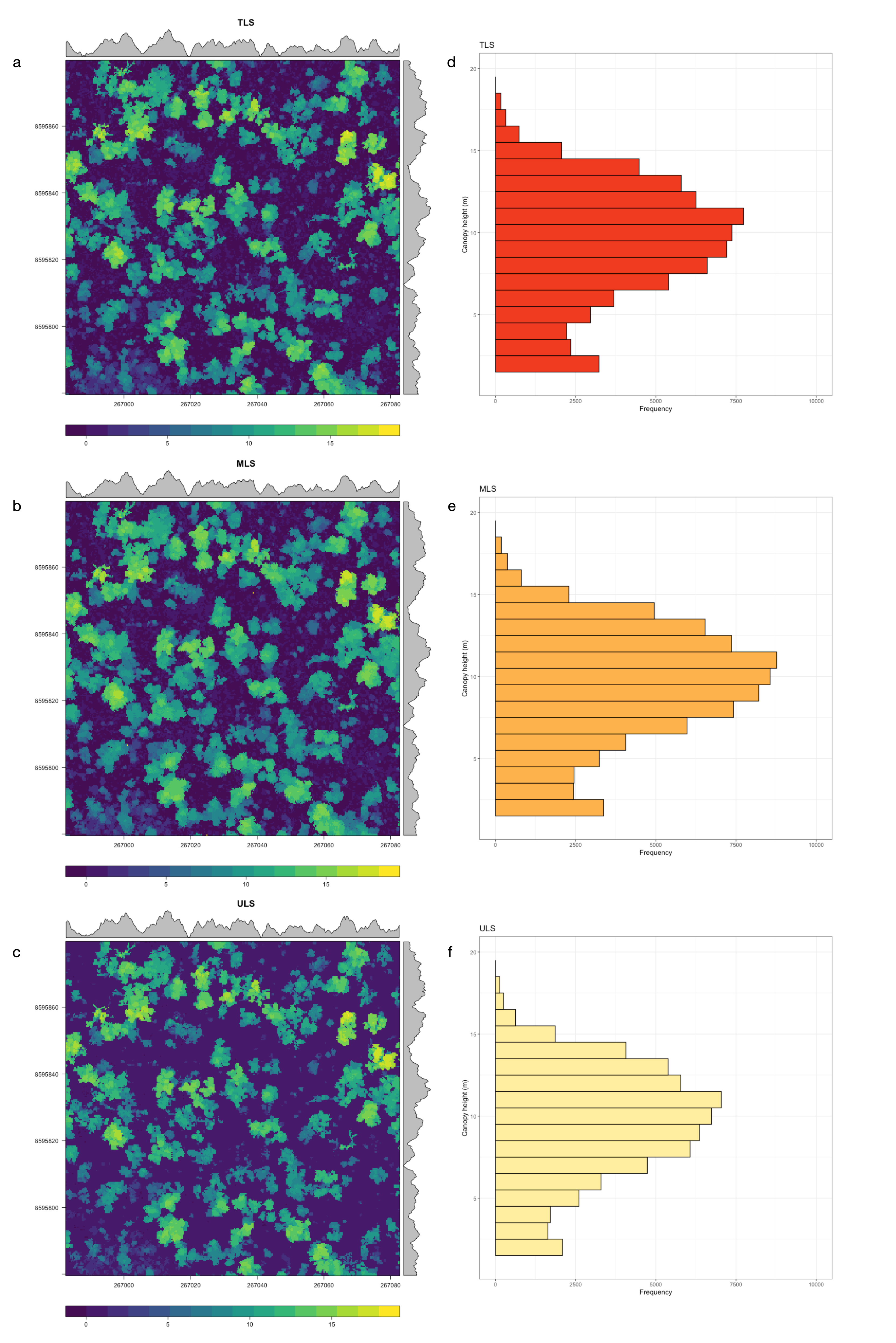
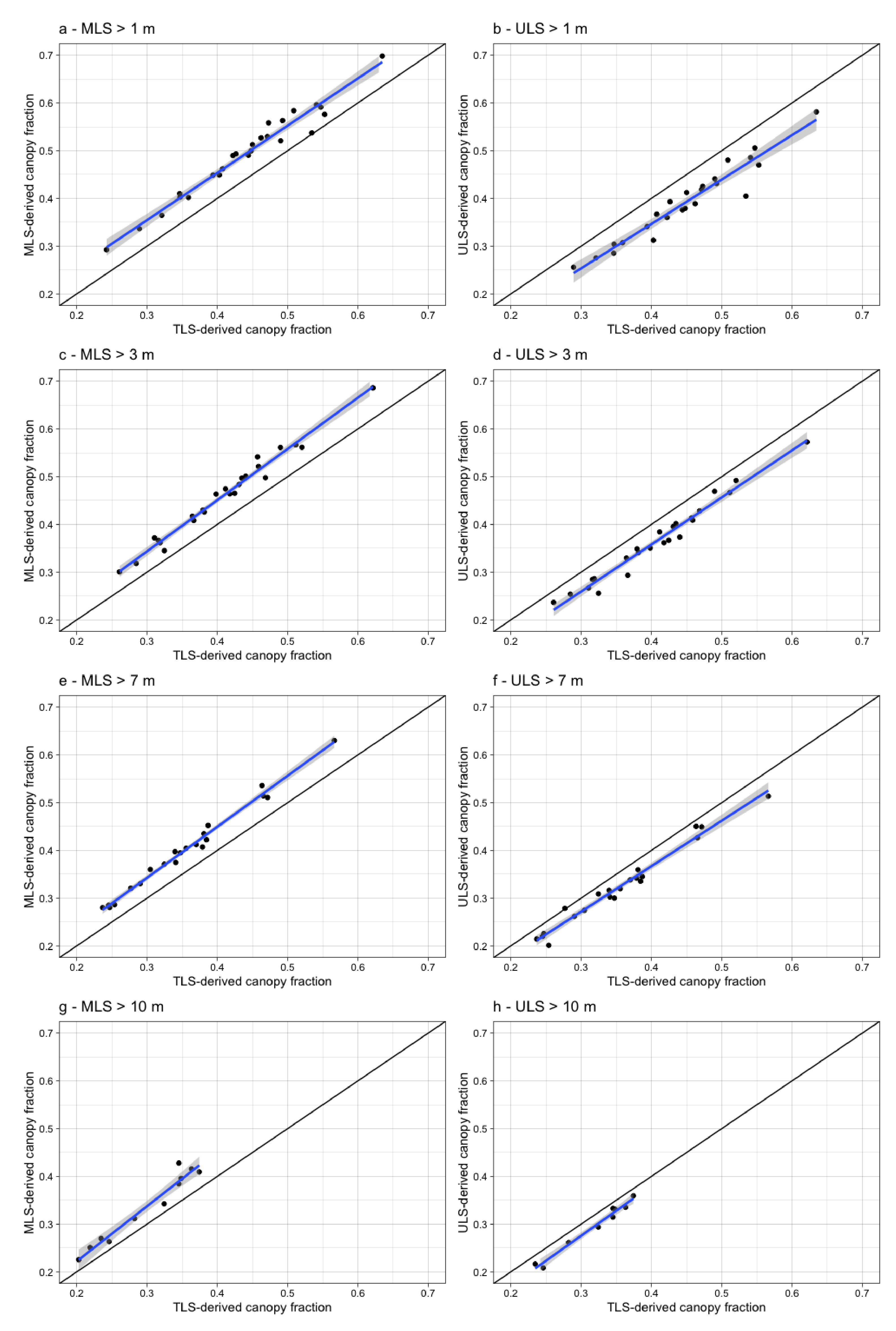
2.5.1. Canopy Characterization

The MLS, and ULS point clouds were finely co-registered to the TLS point cloud using the Iterative Closest Point (ICP) algorithm in CloudCompare [30]. The random sample limit was set to 500,000 and the RMS error difference threshold set to 1 × ${10}^{-05}$, with 100% overlap specified. Ground point classification was conducted with the lasground_new tool in the LAStools suite [31], using -wilderness and -extra_fine settings, and the point clouds were subsequently normalized to height above ground using lasheight. Canopy height models (CHMs) were generated with lasgrid at multiple spatial resolutions using the 95th percentile height. CHM resolution increased in 0.25 m increments from 0.25 m to 5 m resolution to enable a sensitivity analysis of the resolution at which the combinations of the three scanning systems were significantly different. Differences in canopy height distribution derived from the three laser scanning systems was tested across the range of CHM resolutions with the Kolmogorov–Smirnov test [32] in the stats package in R (version 4.0.3).

The 0.25 m resolution CHMs derived from the three scanning systems were used to assess the percentage of woody canopy cover at multiple height class thresholds that represented key strata in the savanna woodland (0.25 m, 3 m, 7 m, 12 m). For each height threshold, median woody canopy cover for 20 m × 20 m subplots embedded in the 1 ha site (n = 25) was compared between TLS-MLS and TLS-ULS with linear regression.

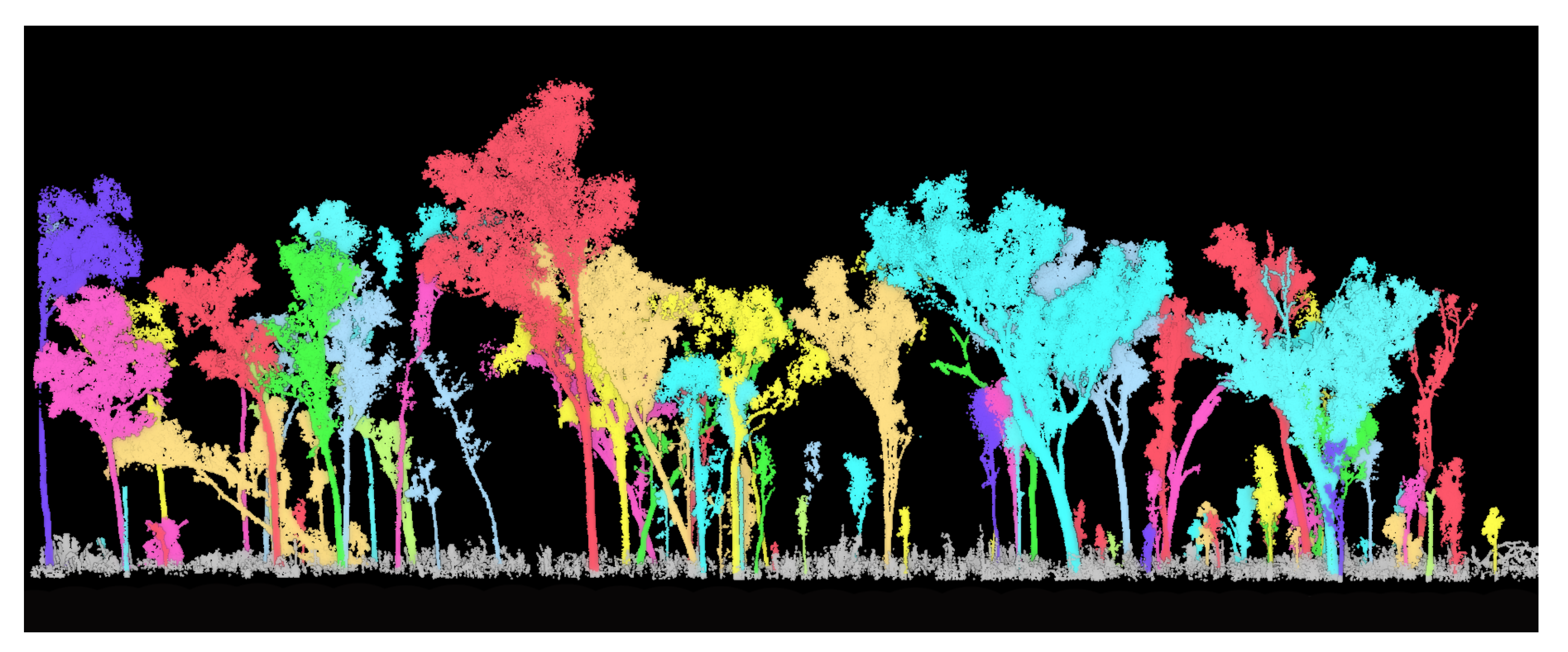
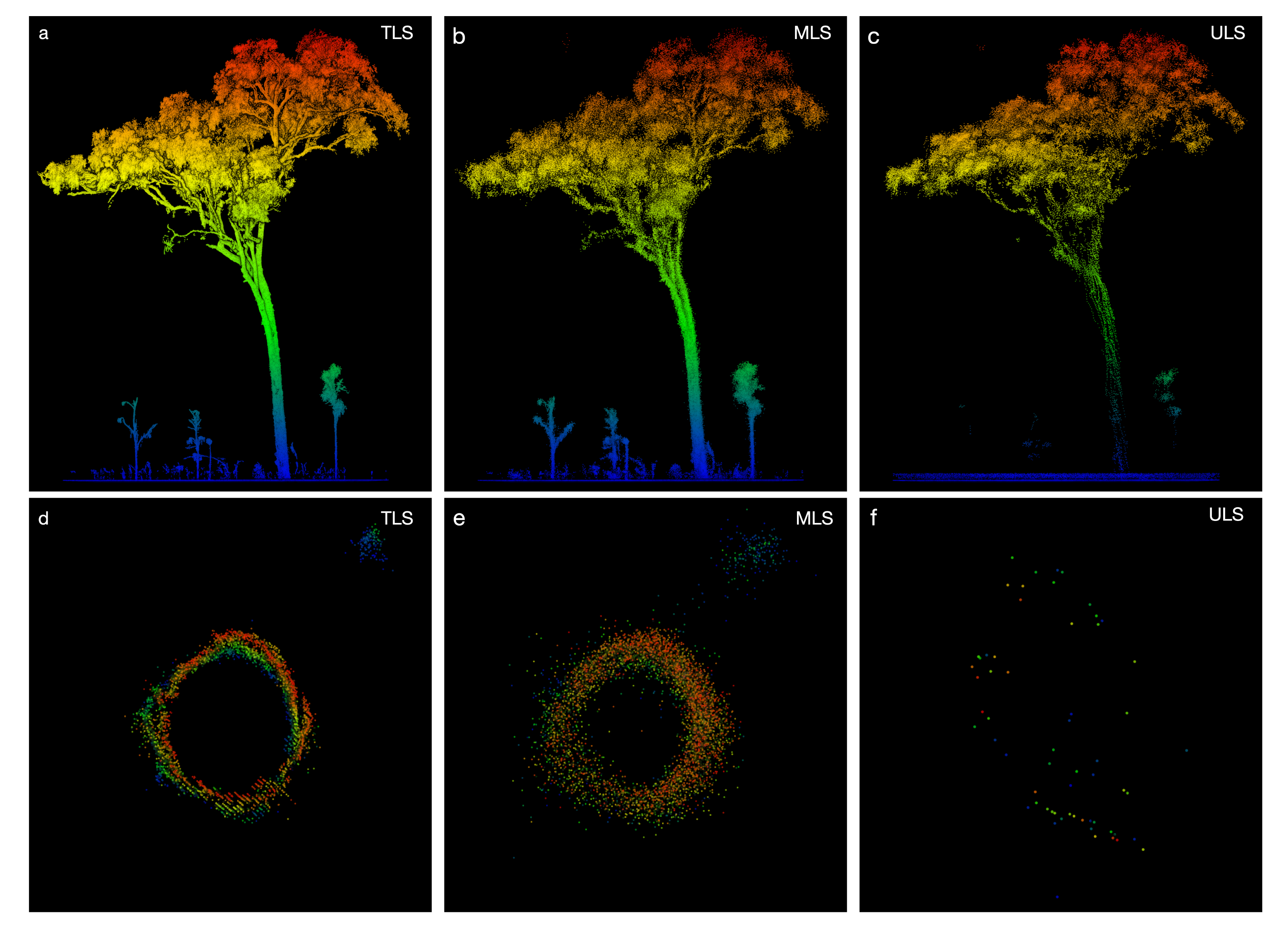
2.5.2. Individual Tree Delineation and Measurement

Individual trees segmentation was applied to the point clouds derived from the three scanning systems using the approach described by [33] and implemented in LiDAR360 (v4.1, GreenValley International) (Figure 3). Results were manually inspected post-segmentation and edited to correct any instances of over- or under-segmentation. Following this quality control checking, the point clouds representing individual trees were processed further in 3DForest (v0.5) to derive individual tree attributes—tree height, crown diameter, crown area, crown volume and stem DBH [34]. An overview of the full processing pipeline is provided in Figure 4.

Above-ground woody biomass (AGB) was estimated at the individual tree level using a set of locally calibrated allometric equations that included the dominant species at the site [35]. AGB was derived from the field inventory as a function of stem DBH (Equation (1), and from the TLS data as a function of stem DBH and tree height (Equation (2)).

$$ln\left(AGB\right)=\beta 0+\beta 1\ast ln\left(D\right)$$

(1)

$$ln\left(AGB\right)=\beta 0+\beta 1\ast ln\left(D\right)+\beta 2\ast ln{\left(H\right)}^2$$

(2)

Multiple linear regression and Random Forest modeling (randomForest [36]), conducted in R, were used to assess the relationship between individual tree biomass (as determined from DBH allometry) and additional measures of tree 3D structure (canopy height, crown area, crown width, crown volume).

3. Results

3.1. Woody Canopy Characterization

All three LiDAR sensing systems provided high quality point-cloud data which captured the three-dimensional structure of the savanna vegetation in rich detail (Figure 5). Viewing the 1 ha plot from an oblique angle, the three point clouds showed very similar structure and it is evident that all three systems captured the canopy patterns well (Figure 5a–c). A cross-sectional slice through the point clouds (5 × 30 m) revealed the narrower beam footprint and higher precision of the TLS instrument, with crisp trunk and branch detail, as well as good definition of material in the herbaceous layer (Figure 5d). The MLS and ULS point clouds were less resolute in comparison, exhibiting some minor noise around tree trunks and evidence of occlusion in the lower stems and herbaceous layer (Figure 5e–f).

The generation of canopy height model (CHM) raster layers confirmed that differences between the three scanning systems was minimal from a visual perspective and displayed very similar spatial patterns of canopy height (Figure 6a–c). Subtle differences were evident, however, and the canopy height distribution ((Figure 6d–f) differed significantly between all three systems at 0.25 m (KS-test, p < 0.001). Sensitivity analysis showed that these differences remained significant until a CHM resolution of 2 m was reached for the TLS-MLS comparisons, and 4 m for TLS-ULS and MLS-ULS comparisons (KS-test, p > 0.05).

Estimation of maximum canopy height was very consistent across the three systems, even at 0.25 m raster resolution. However, the MLS and ULS showed consistent bias in woody canopy cover estimation, over- and under-estimating the woody fraction respectively at multiple height intervals (Figure 7 and

Table 2. Summary statistics of woody canopy attributes collected by the three LiDAR systems at the 1 ha plot scale.

Attribute	TLS	MLS	ULS
CHM max height (m)	18.02	18.65	18.05
Woody canopy cover (%)	51.5	55.3	39.8
Woody canopy cover > 3 m (%)	42.4	46.1	36.9
Woody canopy cover > 5 m (%)	39.9	44.7	34.8
Woody canopy cover > 10 m (%)	18.9	22.1	17.9

).

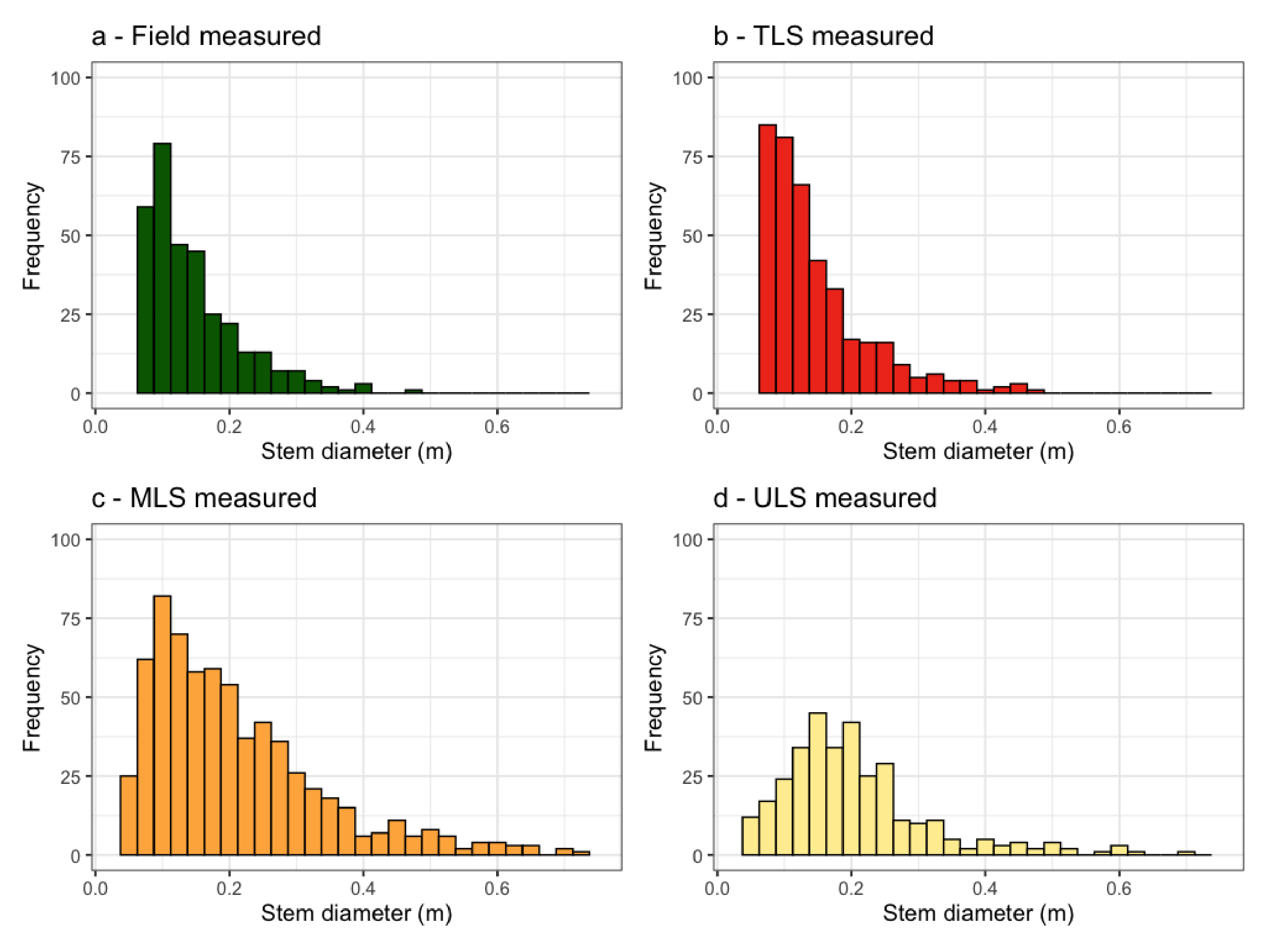
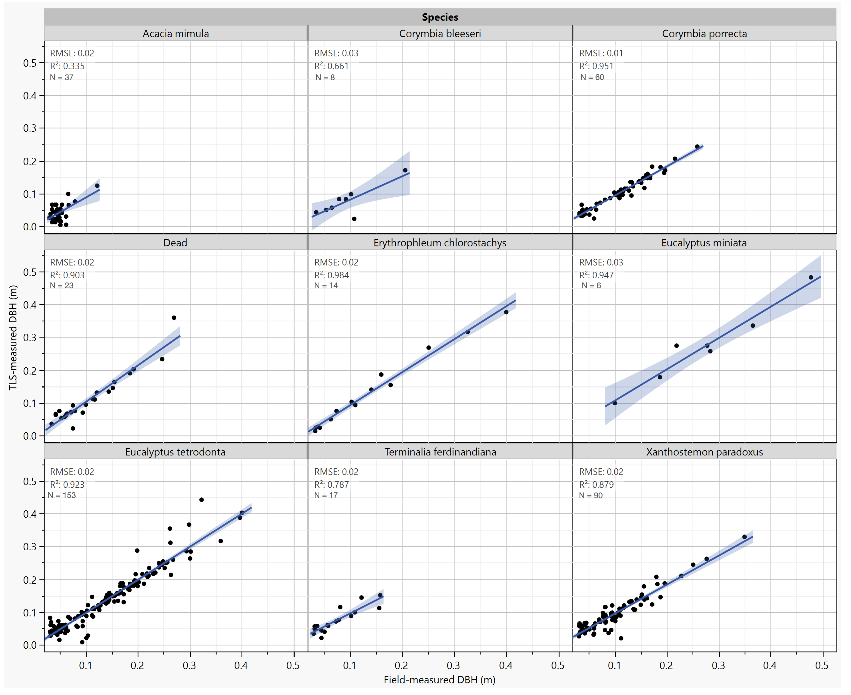
3.2. Individual Tree Characterization

Assessment of 3D structure at the individual tree level highlighted some further distinctions between TLS, MLS and ULS characterization of 3D structure. The TLS capture provided a very clean representation stem, branch and leaf structure, with points spaced close enough together to give the impression of a continuous surface (Figure 8a). Extracting a point-cloud slice from 1.25–1.35 m (to encompass the traditional DBH measurement height) revealed a clear ring of points that allowed for DBH measurement via cylinder fitting (Figure 8d).

The MLS scan captured the general size and shape of individual trees very well, including small under-storey plants, but loss of detail was evident compared to TLS (Figure 8b). The MLS point cloud exhibited more noise around tree stems, which is particularly clear in the thick ring of points extracted at DBH measurement height (Figure 8e). The ULS also captured the general shape of individual trees very well, and although many returns were received from tree stems the density of points in the 1.25–1.35 m range was much lower than from TLS and MLS (Figure 8c,f).

Considering this, we used a broader portion of the tree stems (1–2 m) for cylinder fitting and DBH estimation. Comparison of the DBH distributions against those obtained from the field inventory showed that the TLS estimates closely mirrored the field-measured values (Figure 9a,b), but MLS and ULS estimates (Figure 9c,d) were skewed to larger values and were more normally distributed than the inverse-J patterns evident in the field and TLS data.

Linear regression between field-measured DBH and TLS-estimated DBH confirmed that the TLS could reliably extract individual tree DBH for a broad range of species (Figure 10). Taller tree species with larger sample sizes in the plot such as Eucalyptus tetradonta, Corymbia porrecta and Xanthostemon paradoxus showed the strongest fits (Figure 10), while smaller statured species with narrower DBH ranges exhibited greater error (e.g., Figure 10).

Based on the DBH representation findings discussed above, we restricted our analysis of above-ground woody biomass to the field and TLS datasets. Our field inventory returned a total of 572 stems, corresponding to 41.08 Mg ha${}^{-1}$ of above-ground woody biomass and 20.54 Mg C ha${}^{-1}$ from DBH-based allometry (Equation (1)). Segmentation of the TLS dataset identified almost 100 more stems (n = 669) than measured in the field survey, which were mostly in the smaller size classes (Figure 9b). TLS-estimated biomass, using DBH allometry according to Equation (2), was 7/% greater than the field-inventory estimate at 44.21 Mg ha${}^{-1}$ of above-ground woody biomass and 22.10 Mg C ha${}^{-1}$.

Mapping out the distribution of individual tree biomass spatially showed that field records and TLS predictions were very closely co-aligned (Figure 11a–b). The TLS tree location mapping showed very few instances of omission from field-mapped locations, and a number of commissions which were predominantly located at the very boundary of the plot (Figure 11c). Omissions in the field-inventory mapping along the plot boundary (e.g., south-western corner) are indicative of positioning errors associated with the manual boundary line placement in the field.

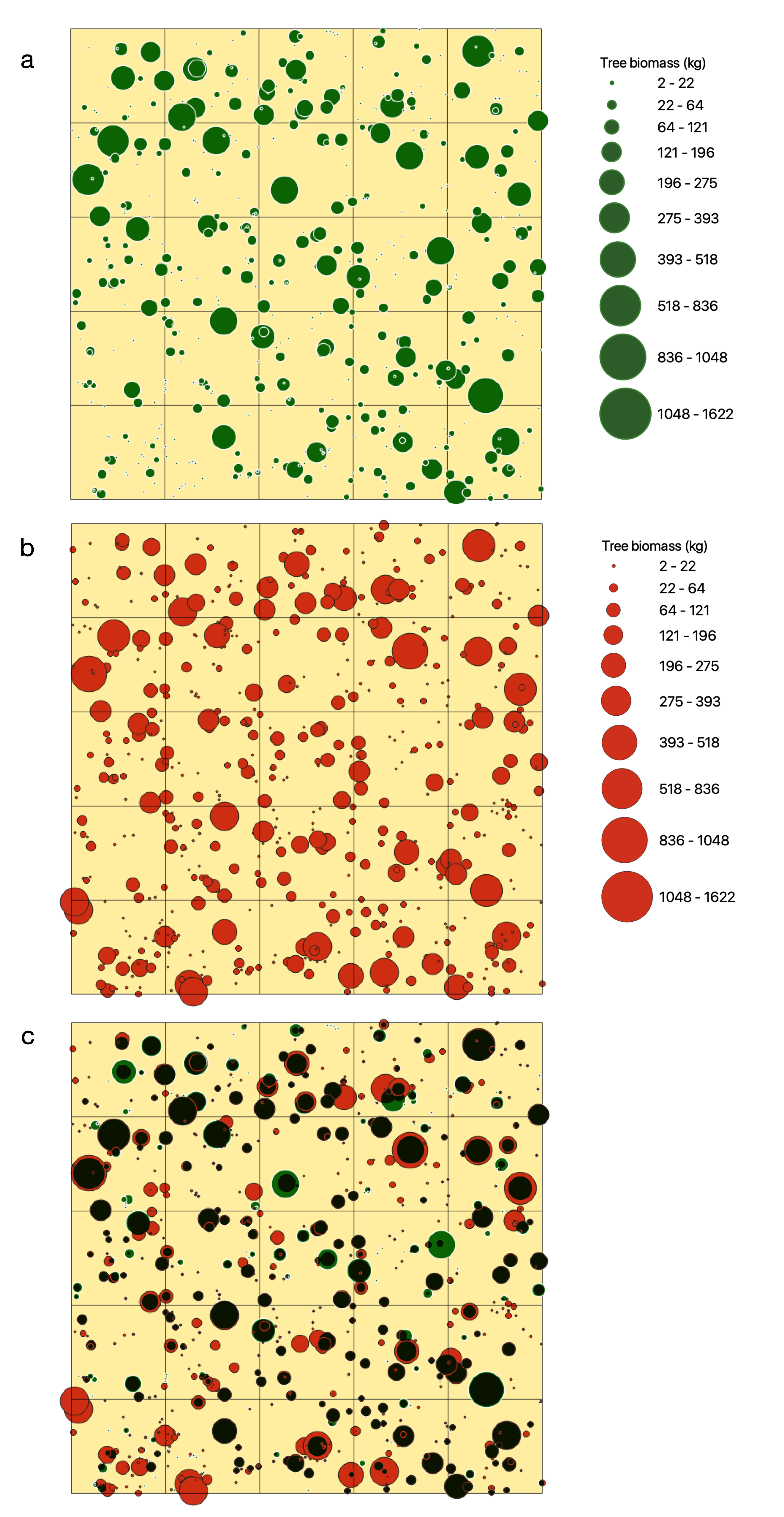
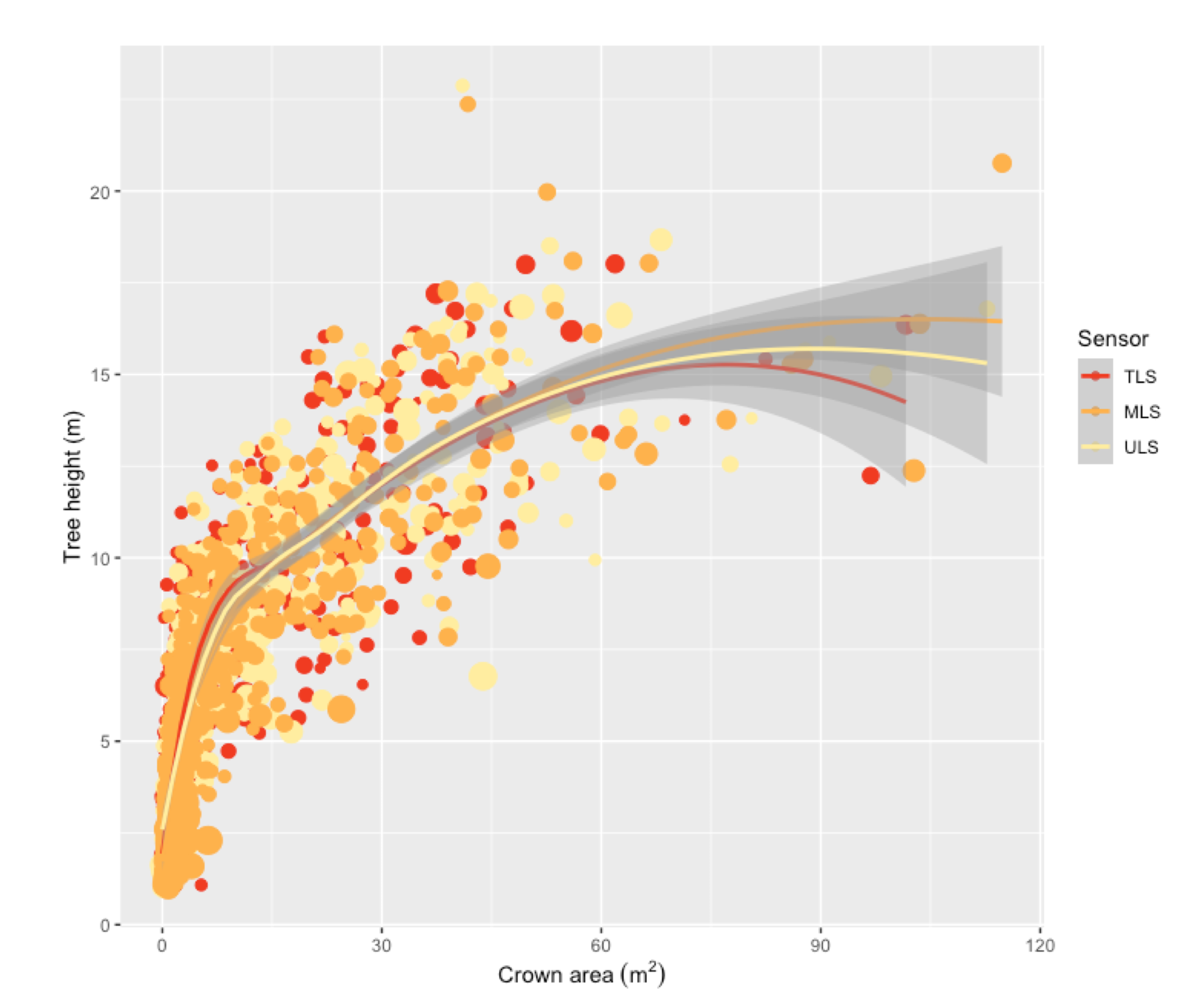
3.3. Allometric Scaling

Given that the MLS and ULS point clouds from our acquisitions were not suitable for direct DBH/AGB retrieval (Figure 9), we explored the possibility of predicting AGB in the MLS and ULS datasets through allometric scaling of tree crown parameters. MLS and ULS captured the general crown structure of individual trees very well (

Table 3. Summary statistics of individual tree attributes collected by the three LiDAR systems.

Attribute	TLS	MLS	ULS
Crown volume max (m${}^3$)	428.37	475.29	406.37
Crown volume mean (m${}^3$)	19.94	23.49	41.67
Crown volume CV (m${}^3$)	2.33	2.29	1.6
Woody biomass (Mg ha${}^{-1}$)	44.21	-	-
Woody biomass (Mg C ha${}^{-1}$)	22.10	-	-

), and the relationship between tree height and crown area that was sensed by the three scanning systems was very consistent (Figure 12). However, both multiple linear regression and Random Forest modeling failed to establish a reliable relationship between canopy attributes and stem DBH/AGB (R${}^2$ = 0.34, RMSE = 0.075 m).

4. Discussion

Laser-based technologies have transformed our ability to measure and monitor savanna vegetation structure. The level of detail and efficiency exhibited in this study from all three sensors is very encouraging from a long-term monitoring and management perspective—providing rigorous baselines from which to assess current state and future dynamics.

4.1. Efficient Monitoring of Habitat Structure

TLS has emerged as the gold standard for 3D characterization of vegetation structure in ecosystems around the globe [17,19]. The high quality results obtained here from TLS are unsurprising, but it is worth noting that the scan position density that we employed (30 m spacing, 16 scans ha${}^{-1}$) was considerably lower than current recommendations in the literature which suggest aiming for 10 m spacing [37]. The TLS literature is heavily skewed towards forested ecosystems where high density scanning is critical for minimizing occlusion. In savanna woodlands and shrublands, which occupy 20% of the global terrestrial surface, the probability of occlusion is much lower and long-range scanners allow for wider scan position placement [20]. This is important in the context of habitat monitoring, as TLS is often considered too time intensive for broad extent and repeat coverage sampling.

Nonetheless, the time required for our TLS survey, and subsequent processing, was still substantially longer than that required for MLS and ULS captures (Table 1). The efficiency of MLS and ULS in terms of time are clear, but do they provide sufficient structural information for ecosystem monitoring? From a canopy height model perspective there is minimal difference among the three scanning approaches and systems. The TLS CHM could not be matched by MLS or ULS at the 0.25 m resolution, but was indistinguishable from MLS at 2 m resolution and ULS at 4 m resolution. For many ecological applications 2–4 m is more than sufficient for providing insight into how canopy growth is tracking over time, and the extended geographic coverage may often outweigh the benefits of finely detailed local structural representation.

The minor under-estimation of woody canopy cover by ULS was consistent across the subplots of our study site. Similar findings have recently emerged from dry sclerophyll forests in Tasmania, where ULS underestimated canopy cover by a few percent in comparison to TLS at the plot scale [38]. Here we show that this under-estimation is a consistent trend across multiple height classes, indicating that the source of this bias is not only under-storey, but also small canopy features such as the edges of branches for example. MLS on the other-hand consistently over-estimated canopy cover in comparison to TLS. This is contrary to the few published studies exploring MLS characterization of woody canopy—which have mostly been conducted in forested ecosystems where tall dense canopy restricts access of the laser beam through to the canopy surface [21,39,40]. In the open savanna woodland of our study, ground-based TLS and MLS can penetrate canopies well with good fields of view. In this instance we attribute the over-estimation of canopy cover by MLS to the nosier point cloud that it produced in comparison to TLS, and these results could likely be improved through further post-processing of the MLS point cloud.

4.2. Individual Trees and Biomass Scaling

Given that MLS and ULS were able to characterize individual tree height and crown attributes very well, albeit with minor bias, we had anticipated that estimation of above-ground biomass would have been possible from these point clouds through allometric relationships with crown attributes. However, our TLS data showed that DBH-AGB did not scale in a predictable manner with tree height, crown diameter, area, and volume (R${}^2$ = 0.36, RMSE = 0.075 m). This was initially surprising in light of how well AGB scales as a function of tree height and crown diameter in many ecoregions around the globe [41], but it is an important reminder of how local-scale variability is averaged out in regional and global syntheses. Savanna eucalypts have notoriously complex crown structures, exacerbated by the actions of fire, termites and cyclone damage [42]. As shown recently in a similar savanna setting in Litchfield National Park, savanna trees exhibit a wide range of crown size variability for a given DBH [6]. In addition to confounding the estimation of DBH and AGB from crown attributes, this variability also brings into question the reliability of using DBH allometry in the first instance for biomass estimation in these systems. The growing use of TLS for building Quantitative Structure Models (QSMs) of trees and accounting for biomass volumetrically has started revealing errors associated with DBH-based allometry in a variety of ecosystem types [43,44] and needs greater exploration in different savanna settings.

4.3. Limitations and Future Directions

TLS is a mature field, with well established protocols for data acquisition and processing [17]. TLS can be deployed in many different ecosystems with high confidence placed in data capture and structural representation, with efficient open-source tools for tree segmentation and structural modeling [45]. Our results obtained from MLS and ULS are encouraging and capture key elements of the savanna woody structure thoroughly. As expected both MLS and ULS did not detect some of the finer-scale ecosystem elements as well as TLS, but are more than sufficient for addressing many ecological questions.

A challenge that arises when comparing different platforms is that the end results are influenced heavily by the acquisition and pre- and post-processing parameters. As such, meaningful generalisations are difficult to make. TLS has the advantage of being a mature technology, with a large user-base and established collection and pre- and post-processing protocols. MLS and ULS are at earlier stages of development and uptake. Furthermore, it is a rapidly expanding industry and a wide variety of sensors and platform exist, from very high-end survey-grade systems (e.g., RIEGL RiCOPTER flying a RIEGL VUX-1) to lighter weight and lower cost options (e.g., DJI M600 with a Velodyne or M8 sensor). Some MLS systems rely solely on SLAM for positioning, while others have integrated RTK-GNSS, so results and noise levels will vary. Additionally, the actual flight/walk patterns and speeds have a marked impact on point-cloud characteristics—and optimal acquisition parameters may be ecosystem specific. Fortunately, since the point-cloud outputs from MLS and ULS share many features of TLS point clouds (at lower densities) analysis of these products can make use of and further advance breakthroughs in TLS processing pipelines.

A key challenge moving forward with MLS and ULS surveying will be to optimize the acquisition and processing parameters in a robust and repeatable manner. We suggest that TLS be leveraged at the start of baseline and long-term monitoring programs to provide a benchmark against which the MLS and/or ULS acquisitions can be optimized. This will enable MLS and ULS to be applied over larger areas and at more frequent time intervals, with intermittent re-calibration against nested TLS collections in key spatial locations and temporal stages throughout the monitoring program. Furthermore, establishing the scaling uncertainty of TLS measurements through to large area ULS surveying will greatly benefit the earth observation community by assisting in the calibration and validation of spaceborne optical, LiDAR and SAR missions (e.g., GEDI, ICESAT-2, NISAR, BIOMASS). When considering the faster acquisition time and the ability to collect data over larger areas, MLS and ULS systems could prove particularly useful for expanding the geographic range and representation of current calibration and validation libraries, with known uncertainties from the nested TLS models.

Lastly, while we have primarily focused here on comparing the individual point clouds and derived products produced through TLS, MLS and ULS surveying, we recognize that much could be gained through their integration. For example, a fused point cloud derived from both TLS and ULS could provide rich vegetation detail from the oblique TLS perspective and comprehensive terrain characterization from the aerial ULS viewpoint.

5. Conclusions

From a canopy modeling perspective, the differences between the TLS, MLS, and ULS were negligible for most applications, but there was a large difference in the acquisition time, with MLS and ULS offering distinct advantages. The trade-off comes through at the individual tree and stem modeling level, where TLS can reproduce DBH estimates from the field with high accuracy and precision, and capture smaller stems than are typically measured in field surveys. Comparisons among TLS, MLS and ULS are challenging as there are a large range of parameters that can be modified across a wide range of applications. TLS surveying is relatively mature, whereas optimal sampling and processing strategies for MLS and ULS are less mature, but rapidly developing. Future research should focus on using TLS as a benchmarking tool to optimize the acquisition parameters of MLS and ULS for a given research and/or management objective. Importantly, this needs to be done across a range of different ecosystem types as the strengths and weaknesses of each sensing system, and platform, will vary with site-specific conditions.

TLS provides a holistic representation of 3D structure that cannot be obtained through traditional field inventory and provides an avenue for optimizing MLS and ULS acquisition parameters, generating correction coefficients for MLS and ULS canopy products, and exploring new allometric models linking point-cloud metrics directly to above-ground woody biomass.

References

1. Gillson, L. Evidence of Hierarchical Patch Dynamics in an east African savanna? Landsc. Ecol. 2005, 19, 883–894. [Google Scholar] [CrossRef]
2. Levick, S.R.; Rogers, K.H. Context-dependent vegetation dynamics in an African savanna. Landsc. Ecol. 2011, 26, 515–528. [Google Scholar] [CrossRef]
3. Levick, S.R.S.; Asner, G.G.P.; Kennedy-Bowdoin, T.T.; Knapp, D.D.E. The relative influence of fire and herbivory on savanna three-dimensional vegetation structure. Biol. Conserv. 2009, 142, 1693–1700. [Google Scholar] [CrossRef]
4. Moncrieff, G.R.; Chamaillé-Jammes, S.; Higgins, S.I.; O’Hara, R.B.; Bond, W.J. Tree allometries reflect a lifetime of herbivory in an African savanna. Ecology 2011, 92, 2310–2315. [Google Scholar] [CrossRef]
5. Woolley, L.A.; Murphy, B.P.; Radford, I.J.; Westaway, J.; Woinarski, J.C. Cyclones, fire, and termites: The drivers of tree hollow abundance in northern Australia’s mesic tropical savanna. For. Ecol. Manag. 2018, 419–420, 146–159. [Google Scholar] [CrossRef]
6. Luck, L.; Hutley, L.B.; Calders, K.; Levick, S.R. Exploring the Variability of Tropical Savanna Tree Structural Allometry with Terrestrial Laser Scanning. Remote Sens. 2020, 12, 3893. [Google Scholar] [CrossRef]
7. Paul, K.I.; Larmour, J.S.; Roxburgh, S.H.; England, J.R.; Davies, M.J.; Luck, H.D. Measurements of stem diameter: Implications for individual- and stand-level errors. Environ. Monit. Assess. 2017, 189. [Google Scholar] [CrossRef]
8. Wulder, M.A.; Coops, N.C.; Roy, D.P.; White, J.C.; Hermosilla, T. Land Cover 2.0. Int. J. Remote Sens. 2018, 39, 4254–4284. [Google Scholar] [CrossRef] [Green Version]
9. Geller, G.N.; Halpin, P.N.; Helmuth, B.; Hestir, E.L.; Skidmore, A.; Abrams, M.J.; Aguirre, N.; Blair, M.; Botha, E.; Colloff, M.; et al. Remote Sensing for Biodiversity. In The GEO Handbook on Biodiversity Observation Networks; Walters, M., Scholes, R.J., Eds.; Springer International Publishing: Cham, Switzerland, 2017; pp. 187–210. [Google Scholar] [CrossRef] [Green Version]
10. Hill, M.J.; Hanan, N.P. Ecosystem Function in Savannas: Measurement and Modeling at Landscape to Global Scales; CRC Press, Taylor and Francis Group: New York, NY, USA, 2010; pp. 1–612. [Google Scholar] [CrossRef]
11. Lefsky, M.A.; Cohen, W.B.; Parker, G.; Harding, D.J. Lidar Remote Sensing for Ecosystem Studies. BioScience 2002, 52, 19–30. [Google Scholar] [CrossRef]
12. Levick, S.; Rogers, K. Structural biodiversity monitoring in savanna ecosystems: Integrating LiDAR and high resolution imagery through object-based image analysis. In Object-Based Image Analysis; Springer: Berlin/Heidelberg, Germany, 2008; pp. 477–491. [Google Scholar] [CrossRef]
13. Colgan, M.S.; Asner, G.P.; Levick, S.R.; Martin, R.E.; Chadwick, O.A. Topo-edaphic controls over woody plant biomass in South African savannas. Biogeosciences 2012, 9, 1809–1821. [Google Scholar] [CrossRef] [Green Version]
14. Levick, S.R.; Richards, A.E.; Cook, G.D.; Schatz, J.; Guderle, M.; Williams, R.J.; Subedi, P.; Trumbore, S.E.; Andersen, A.N. Rapid response of habitat structure and above-ground carbon storage to altered fire regimes in tropical savanna. Biogeosciences 2019, 16, 1493–1503. [Google Scholar] [CrossRef] [Green Version]
15. Davies, A.B.; Asner, G.P. Advances in animal ecology from 3D-LiDAR ecosystem mapping. Trends Ecol. Evol. 2014, 29, 681–691. [Google Scholar] [CrossRef]
16. Stobo-Wilson, A.M.; Murphy, B.P.; Cremona, T.; Carthew, S.M.; Levick, S.R. Illuminating den-tree selection by an arboreal mammal using terrestrial laser scanning in northern Australia. Remote Sens. Ecol. Conserv. 2020. [Google Scholar] [CrossRef]
17. Calders, K.; Adams, J.; Armston, J.; Bartholomeus, H.; Bauwens, S.; Bentley, L.P.; Chave, J.; Danson, F.M.; Demol, M.; Disney, M.; et al. Terrestrial laser scanning in forest ecology: Expanding the horizon. Remote Sens. Environ. 2020, 251, 112102. [Google Scholar] [CrossRef]
18. Liang, X.; Hyyppä, J.; Kaartinen, H.; Lehtomäki, M.; Pyörälä, J.; Pfeifer, N.; Holopainen, M.; Brolly, G.; Francesco, P.; Hackenberg, J.; et al. International benchmarking of terrestrial laser scanning approaches for forest inventories. ISPRS J. Photogramm. Remote Sens. 2018, 144, 137–179. [Google Scholar] [CrossRef]
19. Newnham, G.J.; Armston, J.D.; Calders, K.; Disney, M.I.; Lovell, J.L.; Schaaf, C.B.; Strahler, A.H.; Mark Danson, F. Terrestrial laser scanning for plot-scale forest measurement. Curr. For. Rep. 2015, 1, 239–251. [Google Scholar] [CrossRef] [Green Version]
20. Singh, J.; Levick, S.R.; Guderle, M.; Schmullius, C. Moving from plot-based to hillslope-scale assessments of savanna vegetation structure with long-range terrestrial laser scanning (LR-TLS). Int. J. Appl. Earth Obs. Geoinf. 2020, 90, 102070. [Google Scholar] [CrossRef]
21. Bauwens, S.; Bartholomeus, H.; Calders, K.; Lejeune, P. Forest inventory with terrestrial LiDAR: A comparison of static and hand-held mobile laser scanning. Forests 2016, 7, 127. [Google Scholar] [CrossRef] [Green Version]
22. Corte, A.P.D.; Rex, F.E.; de Almeida, D.R.A.; Sanquetta, C.R.; Silva, C.A.; Moura, M.M.; Wilkinson, B.; Zambrano, A.M.A.; da Cunha Neto, E.M.; Veras, H.F.; et al. Measuring individual tree diameter and height using gatoreye high-density UAV-lidar in an integrated crop-livestock-forest system. Remote Sens. 2020, 12, 863. [Google Scholar] [CrossRef] [Green Version]
23. Kellner, J.R.; Armston, J.; Birrer, M.; Cushman, K.C.; Duncanson, L.; Eck, C.; Falleger, C.; Imbach, B.; Král, K.; Krůček, M.; et al. New Opportunities for Forest Remote Sensing Through Ultra-High-Density Drone Lidar. Surv. Geophys. 2019, 40, 959–977. [Google Scholar] [CrossRef] [Green Version]
24. Brack, C.; Schaefer, M.; Jovanovic, T.; Crawford, D. Comparing terrestrial laser scanners’ ability to measure tree height and diameter in a managed forest environment. Aust. For. 2020, 83, 161–171. [Google Scholar] [CrossRef]
25. Velas, M.; Spanel, M.; Sleziak, T.; Habrovec, J.; Herout, A. Indoor and outdoor backpack mapping with calibrated pair of velodyne lidars. Sensors 2019, 19, 3944. [Google Scholar] [CrossRef] [Green Version]
26. Stal, C.; Verbeurgt, J.; De Sloover, L.; De Wulf, A. Assessment of handheld mobile terrestrial laser scanning for estimating tree parameters. J. For. Res. 2020, 1–11. [Google Scholar] [CrossRef]
27. Prior, L.D.; Whiteside, T.G.; Williamson, G.J.; Bartolo, R.E.; Bowman, D.M. Multi-decadal stability of woody cover in a mesic eucalypt savanna in the Australian monsoon tropics. Austral Ecol. 2020, 45, 621–635. [Google Scholar] [CrossRef]
28. Beringer, J.; Hutley, L.B.; Abramson, D.; Arndt, S.K.; Briggs, P.; Bristow, M.; Canadell, J.G.; Cernusak, L.A.; Eamus, D.; Edwards, A.C.; et al. Fire in Australian savannas: From leaf to landscape. Glob. Chang. Biol. 2015, 21, 62–81. [Google Scholar] [CrossRef] [Green Version]
29. Hernandez-Santin, L.; Rudge, M.L.; Bartolo, R.E.; Whiteside, T.G.; Erskine, P.D. Reference site selection protocols for mine site ecosystem restoration. Restor. Ecol. 2021, 29. [Google Scholar] [CrossRef]
30. Girardeau-Montaut, D. CloudCompare—Open Source Project. Available online: http://www.cloudcompare.org/ (accessed on 10 January 2020).
31. Rapidlasso GmbH. LAStools—Efficient LiDAR Processing Software. 2020. Available online: https://rapidlasso.com/lastools/ (accessed on 12 January 2020).
32. Massey, F.J. The Kolmogorov-Smirnov Test for Goodness of Fit. J. Am. Stat. Assoc. 1951, 46, 68–78. [Google Scholar] [CrossRef]
33. Tao, S.; Wu, F.; Guo, Q.; Wang, Y.; Li, W.; Xue, B.; Hu, X.; Li, P.; Tian, D.; Li, C.; et al. Segmenting tree crowns from terrestrial and mobile LiDAR data by exploring ecological theories. ISPRS J. Photogramm. Remote Sens. 2015, 110, 66–76. [Google Scholar] [CrossRef] [Green Version]
34. Trochta, J.; Kruček, M.; Vrška, T.; Kraâl, K. 3D Forest: An application for descriptions of three-dimensional forest structures using terrestrial LiDAR. PLoS ONE 2017, 12, e0176871. [Google Scholar] [CrossRef] [Green Version]
35. Williams, R.J.; Zerihun, A.; Montagu, K.D.; Hoffman, M.; Hutley, L.B.; Chen, X. Allometry for estimating aboveground tree biomass in tropical and subtropical eucalypt woodlands: Towards general predictive equations. Aust. J. Bot. 2005, 53, 607–619. [Google Scholar] [CrossRef]
36. Breiman, L. Random forests. Mach. Learn. 2001, 45, 5–32. [Google Scholar] [CrossRef] [Green Version]
37. Wilkes, P.; Lau, A.; Disney, M.; Calders, K.; Burt, A.; Gonzalez de Tanago, J.; Bartholomeus, H.; Brede, B.; Herold, M. Data acquisition considerations for Terrestrial Laser Scanning of forest plots. Remote Sens. Environ. 2017, 196, 140–153. [Google Scholar] [CrossRef]
38. Hillman, S.; Wallace, L.; Lucieer, A.; Reinke, K.; Turner, D.; Jones, S. A comparison of terrestrial and UAS sensors for measuring fuel hazard in a dry sclerophyll forest. Int. J. Appl. Earth Obs. Geoinf. 2021, 95, 102261. [Google Scholar]
39. Bienert, A.; Georgi, L.; Kunz, M.; Maas, H.G.; von Oheimb, G. Comparison and combination of mobile and terrestrial laser scanning for natural forest inventories. Forests 2018, 9, 395. [Google Scholar] [CrossRef] [Green Version]
40. Gollob, C.; Ritter, T.; Nothdurft, A. Comparison of 3D point clouds obtained by terrestrial laser scanning and personal laser scanning on forest inventory sample plots. Data 2020, 5, 103. [Google Scholar] [CrossRef]
41. Jucker, T.; Caspersen, J.; Chave, J.; Antin, C.; Barbier, N.; Bongers, F.; Dalponte, M.; van Ewijk, K.Y.; Forrester, D.I.; Haeni, M.; et al. Allometric equations for integrating remote sensing imagery into forest monitoring programmes. Glob. Chang. Biol. 2017, 23, 177–190. [Google Scholar] [CrossRef]
42. Cook, G.D.; Goyens, C.M. The impact of wind on trees in Australian tropical savannas: Lessons from Cyclone Monica. Austral Ecol. 2008, 33, 462–470. [Google Scholar] [CrossRef]
43. Disney, M.I.; Boni Vicari, M.; Burt, A.; Calders, K.; Lewis, S.L.; Raumonen, P.; Wilkes, P. Weighing trees with lasers: Advances, challenges and opportunities. Interface Focus 2018, 8, 20170048. [Google Scholar] [CrossRef] [Green Version]
44. Disney, M.; Burt, A.; Wilkes, P.; Armston, J.; Duncanson, L. New 3D measurements of large redwood trees for biomass and structure. Sci. Rep. 2020, 10, 1–11. [Google Scholar] [CrossRef]
45. Raumonen, P.; Kaasalainen, M.; Åkerblom, M.; Kaasalainen, S.; Kaartinen, H.; Vastaranta, M.; Holopainen, M.; Disney, M.; Lewis, P. Fast Automatic Precision Tree Models from Terrestrial Laser Scanner Data. Remote Sens. 2013, 5, 491–520. [Google Scholar] [CrossRef] [Green Version]
Figure 1. Location of the study site in northern Australia (a), and an aerial view of vegetation cover within the 20 × 20 m subplots of the 1 ha study area (b).
Remotesensing 13 00257 g001
Figure 2. Site conditions at the time of the LiDAR surveys. Occlusion from the grass layer was minimal due to the effects of a fire one month prior.
Remotesensing 13 00257 g002
Figure 3. Cross-section through the TLS point cloud, displaying an example of the individual tree segmentation. Color scheme is a randomised palette.
Remotesensing 13 00257 g003
Figure 4. Overview of the processing workflow and software packages used at different stages of analysis.
Remotesensing 13 00257 g004
Figure 5. Oblique view of the point clouds derived from the three LiDAR platforms: (a) TLS, (b) MLS and (c) ULS. Cross-sectional view of the point clouds derived from: (d) TLS, (e) MLS, and (f) ULS.
Remotesensing 13 00257 g005
Figure 6. Canopy height models derived from the three co-incident LiDAR datasets, plotted at 0.25 m resolution (ac) and their height class distributions (df).
Remotesensing 13 00257 g006
Figure 7. Canopy cover comparisons between MLS and ULS at different height class intervals, against a TLS reference. Solid black is the 1:1 fit.
Remotesensing 13 00257 g007
Figure 8. Example of a single large tree as captured by the three LiDAR systems (ac). Horizontal slice cut through each stem at 1.25–1.35 m above ground level, showing the pattern and density of points available for DBH fitting from each system (df).
Remotesensing 13 00257 g008
Figure 9. Distribution of DBH estimates from field inventory (a) and the three LiDAR approaches (bd).
Remotesensing 13 00257 g009
Figure 10. Comparison of TLS-derived DBH with field-measured values for the dominant woody species.
Remotesensing 13 00257 g010
Figure 11. Spatial distribution of tree biomass as mapped through field inventory (a, n = 572) and from TLS (b, n = 669) using DBH-based allometric equations. Agreement, omissions, and commissions between field and TLS mapping are shown in (c) with overlay blending.
Remotesensing 13 00257 g011
Figure 12. Relationship between individual tree height and crown area, as determined from the three different LiDAR systems.
Remotesensing 13 00257 g012