Abstract
Airborne laser scanning (ALS) acquisitions provide piecemeal coverage across the western US, as collections are organized by local managers of individual project areas. In this study, we analyze different factors that can contribute to developing a regional strategy to use information from completed ALS data acquisitions and develop maps of multiple forest attributes in new ALS project areas in a rapid manner. This study is located in Oregon, USA, and analyzes six forest structural attributes for differences between: (1) synthetic (i.e., not-calibrated), and calibrated predictions, (2) parametric linear and semiparametric models, and (3) models developed with predictors computed for point clouds enclosed in the areas where field measurements were taken, i.e., “point-cloud predictors”, and models developed using predictors extracted from pre-rasterized layers, i.e., “rasterized predictors”. Forest structural attributes under consideration are aboveground biomass, downed woody biomass, canopy bulk density, canopy height, canopy base height, and canopy fuel load. Results from our study indicate that semiparametric models perform better than parametric models if no calibration is performed. However, the effect of the calibration is substantial in reducing the bias of parametric models but minimal for the semiparametric models and, once calibrations are performed, differences between parametric and semiparametric models become negligible for all responses. In addition, minimal differences between models using point-cloud predictors and models using rasterized predictors were found. We conclude that the approach that applies semiparametric models and rasterized predictors, which represents the easiest workflow and leads to the most rapid results, is justified with little loss in accuracy or precision even if no calibration is performed.
Keywords:
LIDAR; mixed-effect models; calibration; point-cloud; raster; semiparametric models; biomass; forest fuels 1. Introduction
Forest fires and carbon accounting are tightly interrelated areas of interest with critical importance for sustainable forest management [1,2]. Detailed spatial information about forest fuels and biomass accumulation in the forest are necessary to guide decision-making processes in these areas [3,4,5]. However, forested areas are typically large and remote, and obtaining this information using only field measurements is an expensive or inefficient option for many applications. For example, national forest inventories, such as the US Forest Inventory and Analysis (FIA) program [6], are able to provide accurate estimates of different forest attributes for large territories such as states or counties using only ground data [7]; however, that level of spatial detail is too coarse to be used in stand-level forest management problems or in fire-behavior simulations.
Prediction of forest attributes using remotely sensed auxiliary information allows obtaining cartographic products with fine resolution with fine resolution, in the range of 10 to 30 m, that can be used in a wide array of forest-management scenarios. In particular, airborne laser scanning (ALS) or airborne LIDAR data provide auxiliary information that is highly correlated with a number of forest structural attributes such as above-ground biomass (AGB), total standing volume, basal area, dominant height, diameter distributions, tree-height distributions, and diversity indexes [8,9,10]. ALS auxiliary information has been shown not to suffer from saturation problems associated with optical datasets such as Landsat imagery when predicting AGB [11,12,13,14,15,16,17]. Furthermore, ALS data have also been used to reliably predict forest fuel attributes that can be used as inputs to fire-spread models [18,19,20].
Besides forest-structure mapping, ALS data can be used for numerous applications such as deriving high-resolution digital terrain models and topographic indices [21,22], mapping human infrastructures [22,23] or improving information about hydrological networks [24,25]. Considering the large set of applications for ALS data, many countries and public agencies have coordinated efforts to obtain state- or country-wide coverage of ALS data. None of the western United States yet have complete ALS data coverage; however, they are continuously increasing their ALS data availability. New ALS data collections in these states cover areas of variable size, which results in a steadily increasing patchwork of areas with available ALS data that capture a broad range of forest conditions [26].
Prediction of forest attributes using ALS data is typically performed using supervised methods that require matching ALS auxiliary information with observations of the target responses taken in field plots without a sizable temporal offset with respect to the ALS data acquisition. The data collected by the FIA program can be used to model forest structural attributes using available ALS data in this manner. However, the discontinuous nature in space and time of the ALS data acquisitions, in combination with the ten-year rotating panel design of FIA in the western US, causes challenges for an operational methodology to produce cartographic products that forest managers can use. Some ALS data acquisition projects are small, such that too few FIA plots are available to perform any modeling exercise. For larger areas, it is possible to develop acquisition-specific models once an ALS data collection is completed. However, modeling requires considerable time and hence delays for the delivery of maps of structural attributes to forest managers—e.g., for fire-related applications—and these delays can imply obtaining inputs for fire-spread simulators only after the fire season has finished. A potential solution to these problems is developing models that can either be: (1) directly transferred to new ALS data collections, or (2) calibrated for new ALS acquisition projects using a potentially small sample size.
Directly transferring a model to a new ALS data collection is a very fast way to generate cartographic products for ALS data acquisitions. As long as the covariates needed for a model are available, generating new maps of forest structural attributes only involves generating predictions from a pre-fitted model. However, this direct transfer, oftentimes referred as synthetic prediction, may involve extrapolations or applying a model to conditions not included in the training dataset, which in turn, can result in significant bias problems. These potential bias problems have been investigated by [27,28,29]. In particular, [28] found bias issues for basal area and stand density when synthetic predictions were respectively used in 33% and 50% of the ALS acquisitions under analysis. A potential solution to these bias problems is localizing pre-existing models to the conditions of a new ALS acquisition through calibration [30]. Calibration is typically based on using mixed-effect models [31] with a fixed component that accounts for the general relationships in the population (i.e., a region) between auxiliary information and response, and a random-effects component that models the variability between subgroups of the population (e.g., particular ALS acquisitions within a region). Once models are fitted, calibrating them to the conditions of a new ALS data acquisition results in a significant reduction in modeling effort because it is only necessary to estimate the random effects for the new ALS acquisition under consideration, which can be done with small sample sizes and eliminates the need to fit new models.
Linear and nonlinear mixed-effects models can be readily calibrated and appear as appealing modeling alternatives to reduce the time needed to obtain maps of forest attributes once a data collection is completed. Nonparametric modeling methods such as k-nearest neighbor imputation [32,33,34], gradient nearest neighbor imputation [35], and random forest [36,37,38] have been extensively used to predict forest attributes from remotely sensed auxiliary information in the last decade. However, the flexibility of these nonparametric methods, that impose no structure in the model errors, makes it impossible to calibrate pre-existing models to new data collections. Nonparametric models can be modified with parametric assumptions about the structure of the model errors [39,40]. These modifications result in semiparametric models that combine flexibility in modeling nonlinear patterns of the nonparametric techniques they are based on, with the possibility of calibrating predictions. Nothdurft et al. [40] proposed combining a k-NN model, fit to obtain population means conditional on a given set of covariates, with a mixed-effects model for the variability not explained by the k-NN model. This method allowed calibrating predictions from the k-NN model to subpopulations of stands. This approach can be applied to the problem of calibrating pre-trained models for new ALS data collections; however, to the best of our knowledge no previous studies exist on this topic.
Finally, models to predict forest attributes from ALS data are typically developed using predictors or metrics derived from the point clouds enclosed in the areas where measurements were taken [41,42]. However, in some operational scenarios direct access to point-cloud data may not be available; i.e., when only gridded summaries of ALS predictors are readily available. Furthermore, sharing gridded products over the internet is more common and demands far fewer resources than sharing point-cloud data. If the accuracy and precision of models developed by extracting predictors for the field plots from pre-rasterized products are not substantially worse than the accuracy and precision of models developed with predictors computed for the point clouds enclosed in field plots, then a workflow entirely based on rasterized products can be a more tractable option for many applications. For example, when modelers do not have the knowledge or technical infrastructure to process point-cloud data, or when it is necessary to unify broad sets of ALS acquisitions. We are not aware of any existing research on this matter, despite the practical justification and need.
This study is developed with the aim of obtaining insights for a regional strategy that allows using information from available ALS data acquisitions for rapid mapping of multiple attributes desired by forest and fuel managers in new ALS project areas. With that overarching objective, we focused our analysis on the state of Oregon and analyzed two sets of response variables. Based on their importance for carbon accounting purposes, the first set of variables consisted of AGB and downed wood biomass (DWB); i.e., the sum of coarse and fine woody debris. The second set of variables contained canopy bulk density (CBD), canopy height (CH), canopy base height (CBH), and canopy fuel load (CFL), chosen because they are inputs for fire-spread models such as Flammap [43,44,45,46] that are widely used by fire and fuel managers. For each response, we analyzed:
- Transferability and effect of calibration. Comparisons focused on analyzing differences in accuracy and precisions between synthetic predictions and predictions obtained using the same models but performing an additional calibration step with available ground and ALS data. We will refer to this factor in the following sections as “calibration”.
- Differences between modeling techniques. Comparisons focused on analyzing differences between parametric linear mixed-effects models and semiparametric models. We will refer to this factor in the following sections as “modeling technique”.
- Differences between models using a different source of ALS metrics. Comparisons focused on analyzing differences between models using ALS predictors computed from point-clouds clipped around the training plot footprints, i.e., point-cloud predictors, and models using predictors extracted from raster layers, i.e., rasterized predictors. We will refer to this factor in the following sections as “source of predictors”.
2. Materials and Methods
2.1. ALS Data Acquisitions and ALS, Climate, and Topographic Metrics
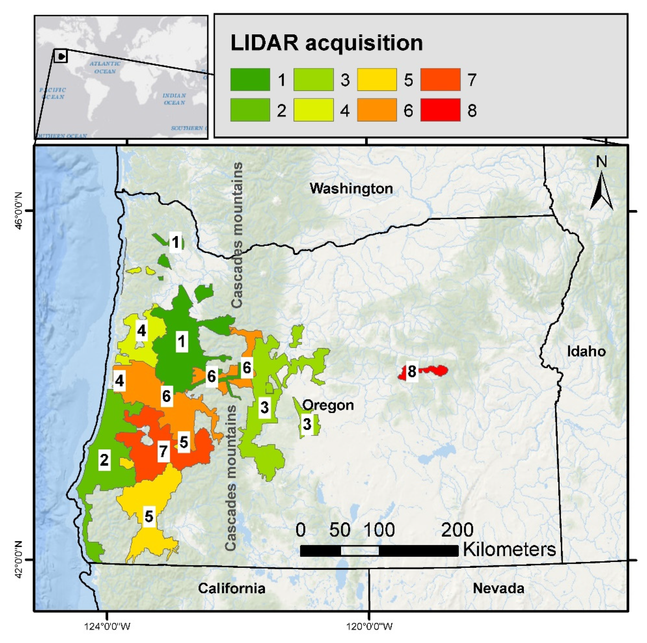
Eight ALS data acquisitions collected by different agencies in the state of Oregon during the period 2008–2016 were used in this study (Figure 1). These acquisitions covered the main forested areas in the state and included areas of temperate coastal coniferous forest, areas with Mediterranean influence in the south of the state, mountain areas on the Cascades range, and drier and more continental forest ecosystems east of the Cascades mountains. The area, completion year, flying altitude, sensor information, return density and number of field plots available for each ALS acquisition are indicated in Table 1.
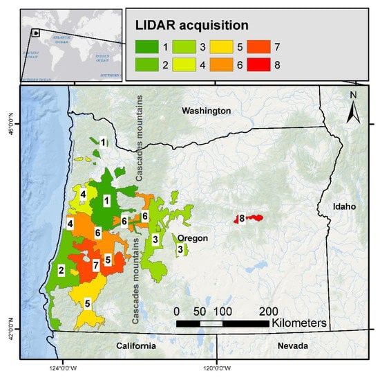
Figure 1.
Study area and airborne laser scanning (ALS) data acquisitions used in the analyses. Individual ALS acquisitions can be identified using Table 1.

Table 1.
ALS data acquisitions summary and number of field plots per ALS acquisition.
For all acquisitions, 30 m resolution rasters containing the ALS metrics indicated in Table 2 were available. The ALS predictors only included descriptors of the distribution of the ALS point cloud such as percentiles or moments and proportions of returns in height categories. For each FIA plot we obtained two sets of ALS predictors. The first set, “rasterized” predictors, was obtained by intersecting the FIA plot center location with the rasters containing the ALS metrics. The second set, “point-cloud” predictors, was obtained by first clipping the points inside the four macro-plots of each FIA plot. Then, for each FIA plot we normalized the point cloud with digital terrain models (DTMs) provided by the vendor of each ALS data acquisition using the R-package lidR [47]. Once normalized, metrics for each FIA plot were computed using FUSION [48]. An extended analysis for the factors: (1) transferability and effect of calibration, and (2) modeling technique, including 12 additional ALS acquisitions where only rasterized predictors were used is presented in Appendix A.

Table 2.
Sets of candidate predictors used in the study.
In addition to the ALS predictors, we used topographic and climate predictors listed in Table 2 in the models for the selected responses. Topographic predictors were derived from a DTM derived from the Shuttle Radar Topography Mission and climate predictors were obtained from the Climate-FVS Ready Data Server [49]. Both topographic and climate indexes were rasterized at a 30 m resolution and a grid that aligned with the grids containing ALS metrics. For each FIA plot, topographic and climate predictors were obtained intersecting the FIA plot center with the corresponding raster layers.
2.2. Ground Data and Response Variables
Ground data to train models was obtained from the FIA database [50]. Coordinates of FIA plots were obtained using mapping-grade GPS units. To the best of our knowledge no study has analyzed directly the reliability of the GPS coordinates of the FIA database in the study area, but based on previous experiences [51,52] the errors are expected to have accuracies in the range of a meter and maximum location errors are expected to be in the range of 5 to 10 m [53]. Following [26], only those FIA plots that were measured at most three years before or after each ALS data acquisition project was completed were used. In addition, any plots presenting any sign of disturbance between the plot visit date and the completion date of their corresponding ALS data acquisition were removed from the dataset. For each one of the remaining FIA plots, AGB per hectare were computed by aggregating tree-level AGB provided in the FIA database with their corresponding expansion factors [50] (Table 3). Estimates of DWB per hectare were obtained for each FIA plot condition class and weighed by the transect length of the appropriate condition class. Finally, values of CBD, CH, CBH and CFL were obtained for the FIA plots using the FireCalc program [54] and the tree-lists of the FIA plots as inputs (Table 3).

Table 3.
ALS data acquisitions and summary of field attributes.
2.3. Parametric Models
Parametric models for AGB, DWB, CBD, CH, CBH, and CFL, were linear mixed-effects models with random intercepts and slopes for each ALS data acquisition. The general form of these models is
where is a p-dimensional vector with the first element a 1 and the p-1 remaining elements being the values of p − 1 covariates for the plot in the ALS data acquisition, is a p-dimensional fixed-effect parameter vector, is a p-dimensional vector of random effects for the ALS data acquisition, and is an additive model error. The random effects were assumed to be normally distributed with a variance–covariance matrix with a vector of variance–covariance parameters that is the same for all ALS data acquisitions; i.e., Model errors were also assumed to be normally distributed, but we allowed for nonconstant error variances. The variance of the model errors was assumed to be proportional to a power of the predictor most correlated with the response, . That is, where and are model parameters that are the same for all ALS data acquisitions. For any pair of ALS data acquisitions, and , random effects and were assumed to be independent so and model errors and for any pair of FIA plots were also assumed to be independent.
Hereafter we will use lower-case Greek letters to denote sets of FIA plots possibly distributed across several ALS data acquisitions. Four sets will be systematically considered in the following sections. The first one, will denote a set of FIA plots used to fit a model, the second one, will be a set of FIA plots or prediction points in an ALS acquisition for which predictions are sought. The third and fourth sets that will be considered are and . The set is the subset of that contains the sampled elements for which both ground and auxiliary information are available. Analogously, is the subset of for which only auxiliary data is known; i.e., the complement of . Letting denote an arbitrary set containing FIA plots, grouped by ALS acquisitions, the model in Equation (1) can be specified in matrix notation as
where is a matrix with rows and columns obtained by stacking the matrices associated to the elements from the ith ALS data acquisition in and is a matrix with rows and columns formed by blocks, where all elements in off diagonal blocks are zeros and blocks in the diagonal are the matrices . The vector of random effects is with and the vector of model errors is with . The variance–covariance matrix of is denoted as where is the variance–covariance matrix of and , the variance–covariance matrix of , a diagonal matrix where the elements in the diagonal equal . Grouping all variance–covariance components into a single vector , we will simplify the notation for as .
2.3.1. Model Selection
A model selection process consisting of four steps was run separately for every response and type of ALS metrics (i.e., point-cloud and rasterized predictors). In the first step we obtained the four linear fixed-effects models with highest R2 with one, two, three, and up to seven predictors using the R-package leaps [55]. For most models we observed that residuals tended to increase with the predicted value, thus, for each candidate we obtained a second fixed-effects model where the error variance was proportional to and compared it to the first model using a likelihood ratio test. When the p-value of the likelihood ratio test was smaller than 0.05, the candidate model with constant error variance was replaced by its counterpart with error variance proportional to . Finally, for each candidate we obtained a mixed-effects model having the same fixed effects and error variance but incorporating random effects as indicated in Equation (1). The significance of the fixed-effect coefficients associated with each predictor was tested for each candidate and those coefficients that were not different from zero at a 0.05 significance level were sequentially removed from the model until all fixed effects were significantly different from zero at a 0.05 confidence level. The result was a list of 28 models from which we selected a final one for the response variable under consideration.
To select the final model, we first removed from the list of 28 candidates all models where the maximum variance inflation factor, VIF, was larger than 5. To balance parsimony and predictive power, we observed at the increases of explained variance when increasing the number of predictors. We initially removed from the list all models where the R2 was 2.5% less than the maximum. Then, we only kept the models with the smallest number of predictors and selected the model with lowest root mean square error if more than one remained in the list. All models in this process were obtained using maximum likelihood and functions from the R package nlme [56].
2.3.2. Prediction and Calibration with Parametric Models
Once models were fitted, we obtained synthetic predictions and calibrated predictions for each FIA plot. Letting be the estimated variance–covariance parameters of the model, we obtained the estimated fixed-effect parameters as
Synthetic predictions for points in a new ALS acquisition, , were obtained by a direct extrapolation using the fixed-effects parameters obtained in the model fitting stage as
To emphasize that these are synthetic predictions, we will use the superscript . It is important to note that synthetic predictions do not perform any calibration to the local conditions of a new ALS data acquisition and can be obtained without any new ground information.
If a set of ground observations with their corresponding values of the auxiliary variables is available for the new ALS data acquisition, then, following p. 314 [57], it is possible to obtain calibrated predictions as
where the superscript is used to denote that these are calibrated predictions and
2.4. Semiparametric Models
For each response variable we obtained semiparametric random-forest models using point-cloud and rasterized predictors. We followed the approach proposed by [40] but included some modifications to accommodate nonconstant error variances because increasing error variances are commonly observed when modeling forest attributes with ALS auxiliary information (e.g., [58,59]).
The form of the semiparametric models can be described as
where is a fixed and unknown function that will be approximated by the random forest algorithm and a random variable with zero mean that includes all the variation that is not explained by .
We further assumed that the random component not explained by was
where is a random effect specific of the ALS data acquisition and is an additive model error for the plot in the ALS acquisition. Random effects and model errors are assumed to be independent of each other and normally distributed with , where , , and are model parameters. Finally, was assumed to be independent of for any pair of ALS data acquisitions and independent of for any pair of FIA plots.
For an arbitrary set of units, model (8) can be expressed as
where is a dimensional column vector obtained stacking the values of all units in and is a matrix with rows and columns, where the row corresponding to the element of the acquisition has zeros everywhere except for the position, which has a value of . The vector groups the random effects for all ALS acquisitions in and the vector is a vector of model errors obtained in the same way as . The variance–covariance matrix of is with an identity matrix of dimension and the variance–covariance matrix of is . Letting be the variance–covariance matrix of , we have
Variance–covariance parameters , , and were obtained after a random forest model was fitted to the training sample . Then we assumed that the random forest provided a close approximation, , to the unknown function . Using we obtained , which were assumed to have a normal distribution with zero mean and variance covariance matrix as indicated in Equation (10). The estimated residuals from the random forest model, , were finally used to estimate , and using maximum likelihood.
2.4.1. Model Selection
A model selection consisting of three steps was developed for every response variable and source of ALS metrics. In the first step we followed the approach described by [28] and eliminated correlated predictors using the QR decomposition implemented in the multi.collinear function of the rf.Utilities R package [60]. This step was run only once for each combination of response variable and source of ALS metrics. In the second step, we used the function rf.modelSel [60] to identify the best combination of variables selected in the final random-forest model for each response variable and source of ALS metrics. Once predictors were selected, random-forest models were fit using the randomForest R package [61]. These models provided the nonparametric component of the semiparametric models and were used to compute values for . In the last step, we obtained the parametric part of the model that e×plains differences in due to ALS acquisition membership. Two models as indicated in Equation (10) were obtained for the variance–covariance of random effects and model errors using the R package nlme [56]. The first model had a fixed exponent ; i.e., homoscedastic errors, and the second model had an exponent that was free to vary during the model-fitting stage. Both models were compared using a likelihood ratio test. We selected the model with variable when the p-value of this test was smaller than 0.05; otherwise, we selected the model with .
2.4.2. Prediction and Calibration with Semiparametric Models
A direct application of the random forest model to a new ALS data acquisition provides synthetic predictions
Following [41] (pp. 307, 353), calibrated predictions can be obtained as
with
2.5. Accuracy Assessment and Comparisons
2.5.1. Cross-Validation and Performance Metrics
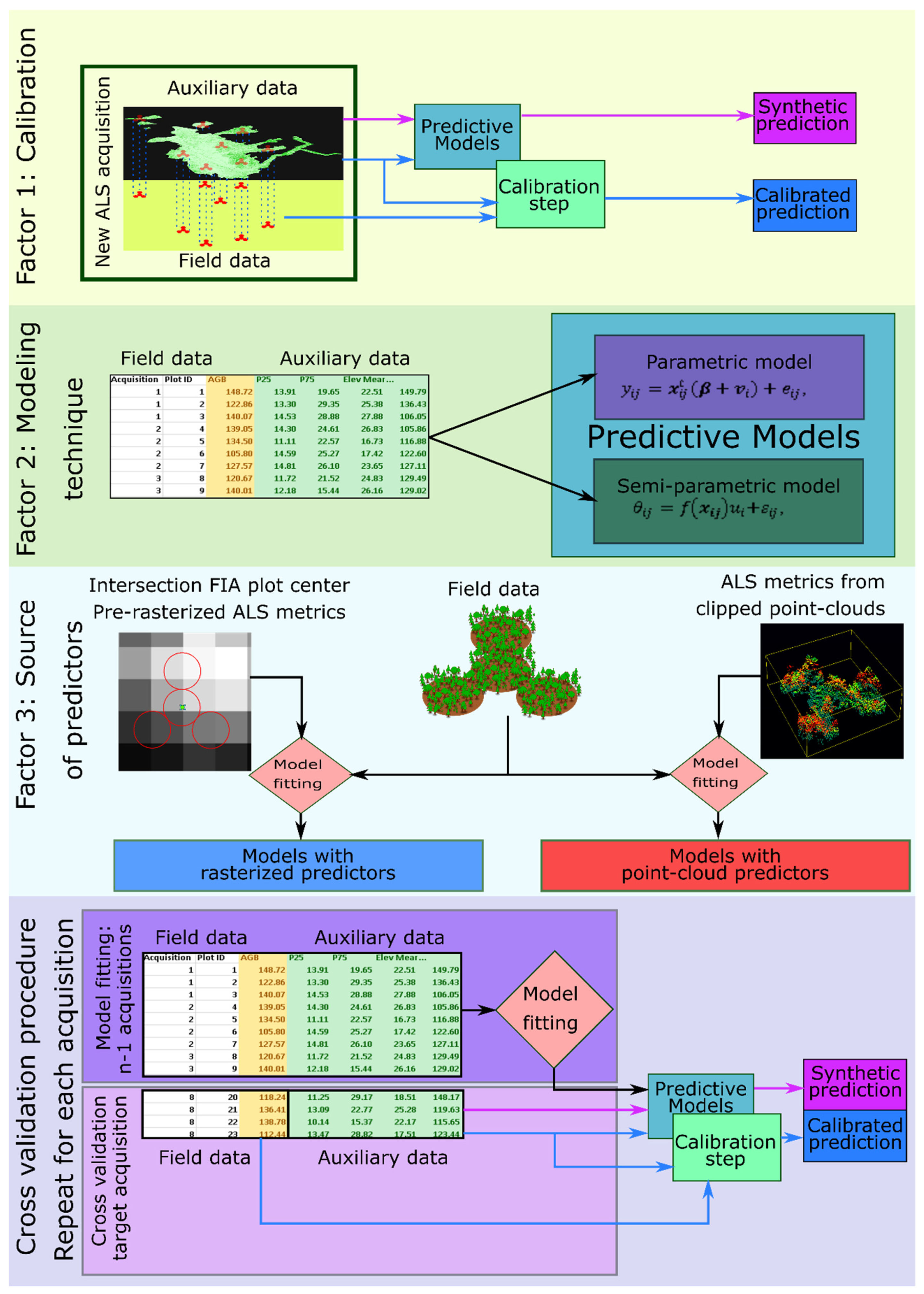
To assess the effect of calibration for new ALS data acquisitions, we used the following procedure for each response variable and modeling technique (Figure 2). First, for each ALS data acquisition, we split the entire training dataset in two parts, and . The set , the training subsample, contained all FIA plots not included in the selected ALS data acquisitions, and the set contained the FIA plots within the ALS data acquisition under consideration. Models obtained in the model selection stage were re-fitted using only and synthetic predictions were obtained for all elements in . Finally, random effects and calibrated predictions for parametric and semiparametric models were obtained using Equations (5) and (6) and Equations (12) and (13), respectively. To consider that only FIA plots measured prior to the acquisition date will be available for the calibration of new ALS data collections, we performed the calibration using , the subset of that contained the FIA plots that were measured the year the ALS data acquisition was finished or the three previous years. It is important to note that while models were selected including also plots measured up to three years after the ALS data collection was finished, we tested the effects of the calibration by excluding the plots that were measured after the ALS data collection was finished when computing the random effects using Equations (6) and (13). The potential use of the models developed in this study is to perform calibrations in new ALS data acquisitions. Thus, excluding the plots that were measured after the acquisitions were finished provides a closer approximation to the sample sizes that could be used for calibration in a real case. The result of this process was (1) a set of synthetic predictions from models developed with data from different acquisitions and (2) a set of calibrated predictions where only the field plot data available at the end of the ALS acquisition project was used to compute random effects.
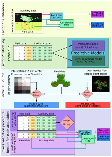
Figure 2.
Schematic representation of the three factors analyzed in this study, the computation of ALS metrics and the cross-validation procedure. ALS: Airborne Laser Scanning. FIA: Forest Inventory and Analysis.
We used both sets of predictions to compute and obtained the following performance metrics:
where represents the number of elements in the ALS data acquisition and can represent synthetic or calibrated predictions. In addition to these metrics we also computed their values relative to the mean, , of the response variable under consideration as:
And the coefficient of determination as:
2.5.2. Differences between Calibrated and Synthetic Predictions, Modeling Techniques, and Sources of ALS Metrics
For each response variable, we analyzed changes in performance due to each of the three factors under analysis (Figure 2) by computing changes in the relative root mean square error and relative bias. For a given factor, changes were computed as:
and:
where , and are generic superscripts that respectively indicate the factor under analysis and the two alternatives that are compared. For the transferability analysis we used the symbol for , and for calibrated predictions and for synthetic predictions. To analyze differences due to the modeling technique we used error metrics computed after performing the corresponding calibration. We used the symbol to indicate the factor “modeling technique”, and for the parametric models and for the semiparametric models. Finally, for the comparisons of models using rasterized and point-cloud ALS predictors, error metrics were also computed after performing the corresponding calibration. The letter was used to indicate the factor “source of predictors”, and for models using rasterized ALS metrics, and for models using point-cloud predictors.
To test differences in model performance due to: (1) the modeling technique and (2) the source of ALS metrics, we used a t-test on the differences to test differences in accuracy and a t-test on the differences to assess differences in precision. Finally, in addition to the global values of , and , these metrics were also computed for each ALS acquisition separately.
3. Results
3.1. Parametric and Semiparametric Models
Regardless of the source of ALS metrics and modeling technique, several patterns were observed with respect to the predictive performance of the models for different response variables. The largest values were obtained for CH, followed by AGB, with values ranging from 88.59% to 85.29% and from 80.03% to 76.45%, respectively. For the remaining variables the explanatory power of the models was largest for CFL with values above 50%. This variable was followed by CBH and CBD, which tended to have values around 30% and 25% respectively. Finally, the explanatory power of the models for DWB was very poor, and larger for the parametric models where reached 13.79% for the model using point-cloud metrics and 13.49% for the model using rasterized predictors. Patterns observed for were similar to those observed for but in the opposite direction. Finally, was positive for most models indicating a systematic overprediction with a magnitude that varied substantially between variables. For CH and AGB it was below 2.5% in absolute value. For CBD, CBH, and CFL, was below 10% in absolute value and for DWB exceeded 5% for the parametric models and 15% for the semiparametric models (Figure 3).
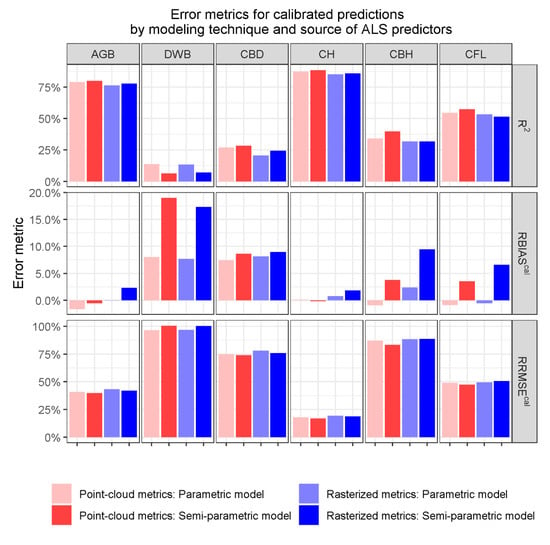
Figure 3.
Relative root mean squared error (RRMSEcal), relative bias (RBIAScal), and coefficient of determination (R2) for parametric models. Error metrics were calculated for models fitted with the entire dataset under consideration and predictions calibrated using all plots in the corresponding ALS acquisition, which were measured either in the year that the ALS data acquisition was finished, or in the two previous years. Model response variables are: aboveground biomass (AGB), downed woody biomass (DWB), canopy bulk density (CBD), canopy height (CH), canopy base height (CBH), and canopy fuel loading (CFL).
All models included random effects; however, for the parametric models for DWB and CBH using point-cloud predictors, the inclusion of random effects did not improve the model fit significantly at a 0.05 confidence level. For CBH the model selection algorithm for the parametric models described in Section 2.3.1 provided models with up to six predictors, followed by models with three predictors but with an R2 3.2% points larger than the maximum R2. These simpler models were considered more appropriate and selected as final models for this variable because they allowed for a substantial model simplification without causing important performance losses. For most variables, sources of ALS metrics, and modeling techniques, models improved when including random effects for the ALS acquisitions and a parameter to account for nonconstant error variances (Table A4, Table A5 and Table A7). The only exceptions to this trend were the parametric models for CFL and the parametric model for CH using rasterized ALS metrics.
Important differences were observed between parametric and semiparametric models for the number of predictors included in the model. The median number of predictors for the semiparametric models was 33, and ALS, topographic, and climate metrics were present in all but the semiparametric model for DWB using rasterized predictors. The median numbers of ALS metrics, topographic, and climate metrics were 18, 10, and 4 variables respectively (Figure A5). Parametric models always had less than five predictors and in most cases these predictors were derived from the ALS data (Table A4 and Table A5).
3.2. Differences between Synthetic and Calibrated Predictions
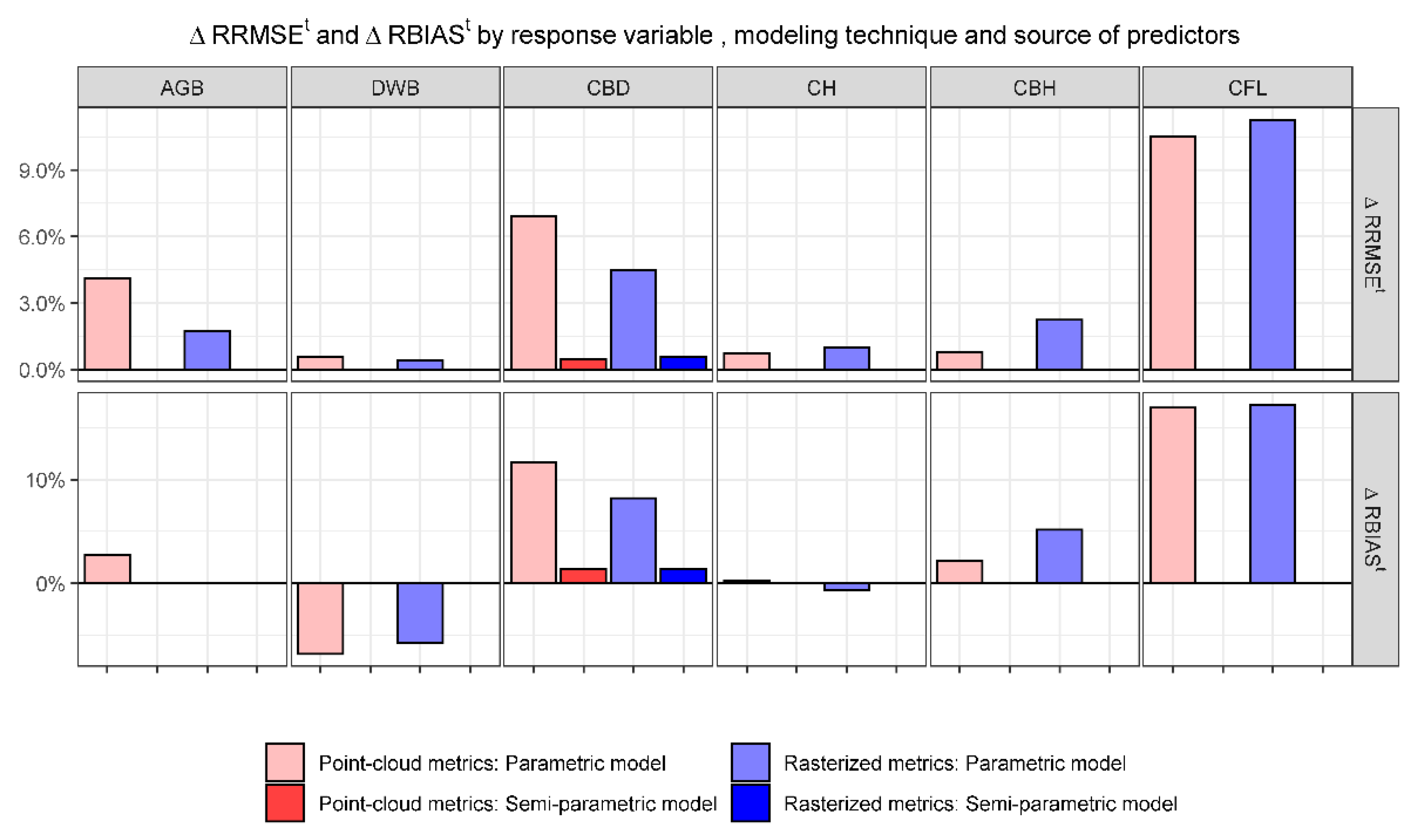
All models included ALS acquisition random effects; however, the magnitude of these effects varied significantly between variables and modeling techniques. For semiparametric models, reductions in global and were negligible, which indicates that with these models using synthetic predictions and omitting the calibration step will not have consequences of practical importance in accuracy and precision. While semiparametric models seem to capture differences between ALS acquisitions directly, leaving little room for improvements to the calibration stage, parametric models operate differently, and their performance improves substantially with the calibration. Parametric models captured the main relationship with auxiliary information in their fixed-effect component, and a part of the variability between ALS acquisition was accounted for in the calibration stage (Figure 4). Focusing on the parametric models, for AGB, CBD, CBH, and CFL calibration resulted in consistent reductions of the global and . For DWB and CH, three parametric models failed at reducing the global . We further inspected this issue by looking at ALS-acquisition-specific values of for the parametric models.
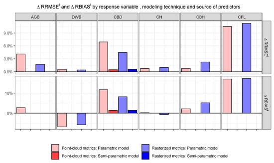
Figure 4.
Changes in relative root mean square error and relative bias due to calibration. Positive values indicate improvements. AGB, DWB, CBD, CH, CBH, and CFL respectively indicate aboveground biomass, downed woody biomass, canopy bulk density, canopy height, canopy base height, and canopy fuel load.
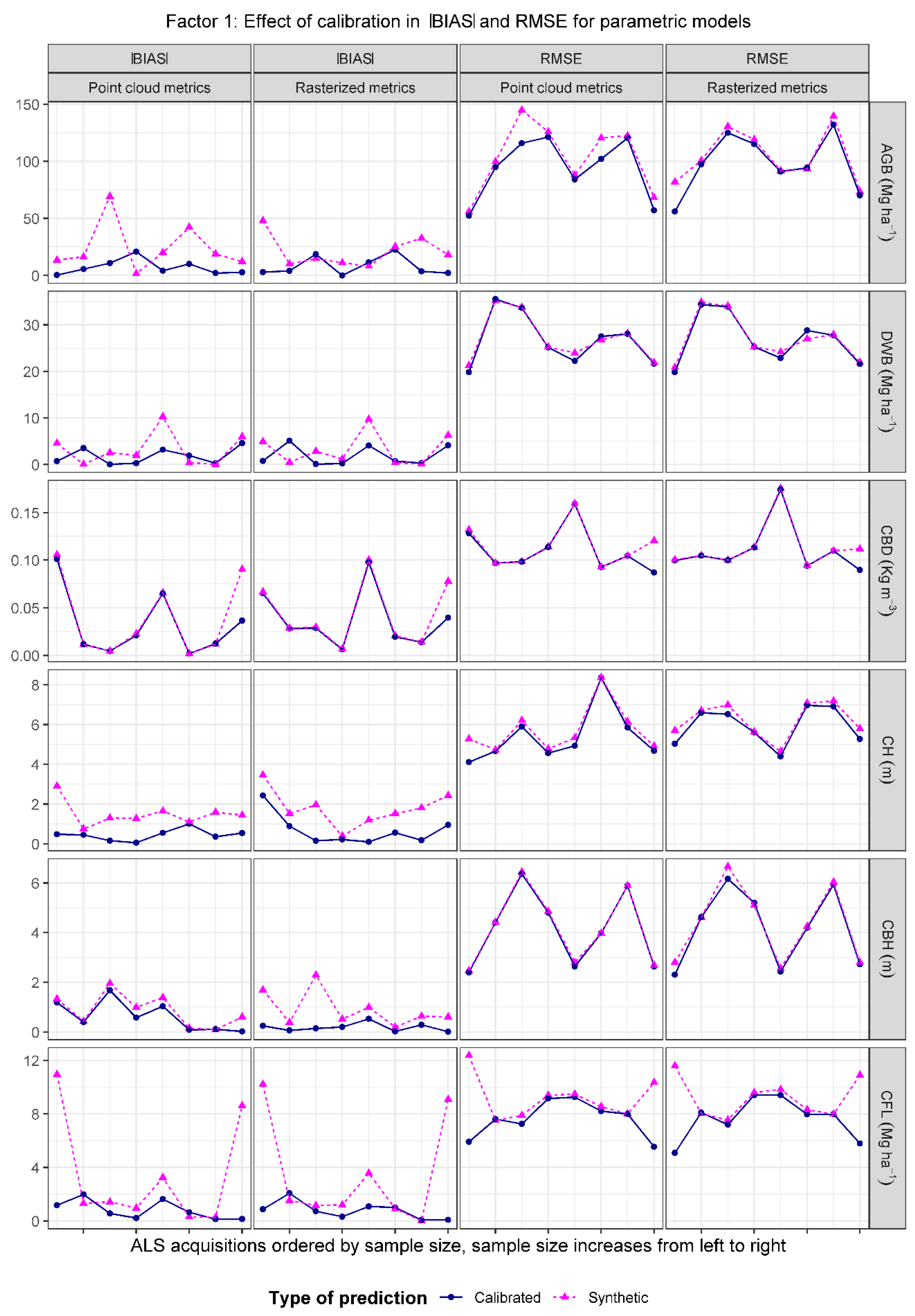
For all variables and source of ALS metrics the decreased in the majority of the ALS acquisitions after the calibration was performed (Figure 5). These reductions in the ALS acquisition also resulted in a reduction of . Similar patterns were observed for the e×tended dataset using only rasterized metrics (Figure A3). The effect of the calibration in DWB was very small and erratic, which, in conjunction with the poor performance of the models for this variable, indicate that the variability in DWB cannot be predicted well by the auxiliary information used in this study or by geographic factors such as membership in a particular ALS acquisition area. For the remaining variables the effect of the calibration varied in magnitude depending on the variable and source of predictors. Most important effects of calibration were observed for CH followed by CBH and AGB, and the smallest reductions of ALS-specific were observed for CBD. Overall, the calibration step had positive impact in reducing the ALS acquisition biases and that is the main advantage of the mixed-effects parametric models developed in this study.
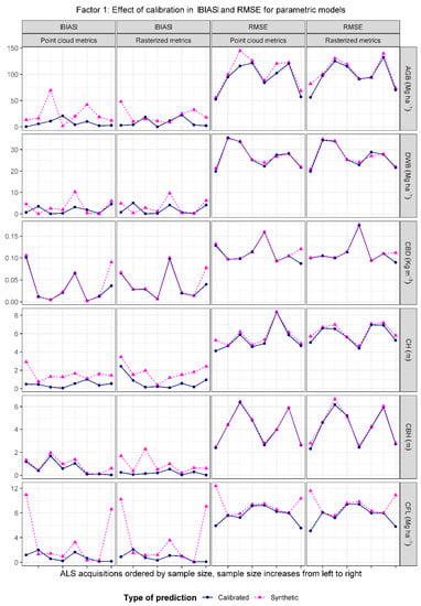
Figure 5.
Absolute value of bias, , and root mean square error, , for synthetic and calibrated predictions of parametric models by ALS data acquisitions. AGB, DWB, CBD, CH, CBH, and CFL respectively indicate aboveground biomass, downed woody biomass, canopy bulk density, canopy height, canopy base height, and canopy fuel load.
3.3. Differences between Parametric and Semiparametric Models
Parametric models provided lower values of the global in 11 of the 12 possible combinations of response variables and sources of ALS metrics, while semiparametric models provided lower values of the global in 8 of the 12 possible comparisons. With the exception of DWB, for which parametric models provided consistently better results in terms of and , there was no modeling technique that can be considered as clearly superior than the other. For DWB, CBD, CH, CBH, and CFL, the of parametric models was smaller than the bias of their semiparametric counterparts regardless of the source of ALS predictors (Table 4). For AGB there was no modeling technique better than the other in terms of . Semiparametric models provided better results in terms of global for AGB, CBD, and CH, while for DWB the parametric models had consistently smaller values of . The magnitude of the differences in and between parametric and semiparametric models were of small magnitude for those responses with larger . For CH and AGB, differences between modeling techniques in and in were below 1.35% and 2.27% respectively, regardless of the source of ALS metrics. Excluding DWB, magnitude of the differences in were most important for the models for CBH and CFL using rasterized predictors, while differences in were below 4% for all variables (Table 4). Similar results were obtained when comparing parametric and semiparametric models with an extended dataset that included 12 additional ALS acquisitions (Table A3). The smaller of the parametric models and smaller in semiparametric models clearly indicates performance tradeoffs between modeling techniques; however, the magnitude of these tradeoffs is for most variables of very small magnitude.

Table 4.
Differences between parametric and semiparametric models. AGB, DWB, CBD, CH, CBH, and CFL respectively indicate aboveground biomass, downed woody biomass, canopy bulk density, canopy height, canopy base height, and canopy fuel load. Superscripts and indicate error metrics for parametric and semiparametric models respectively and the superscript denote changes in and due to using a different modeling technique.
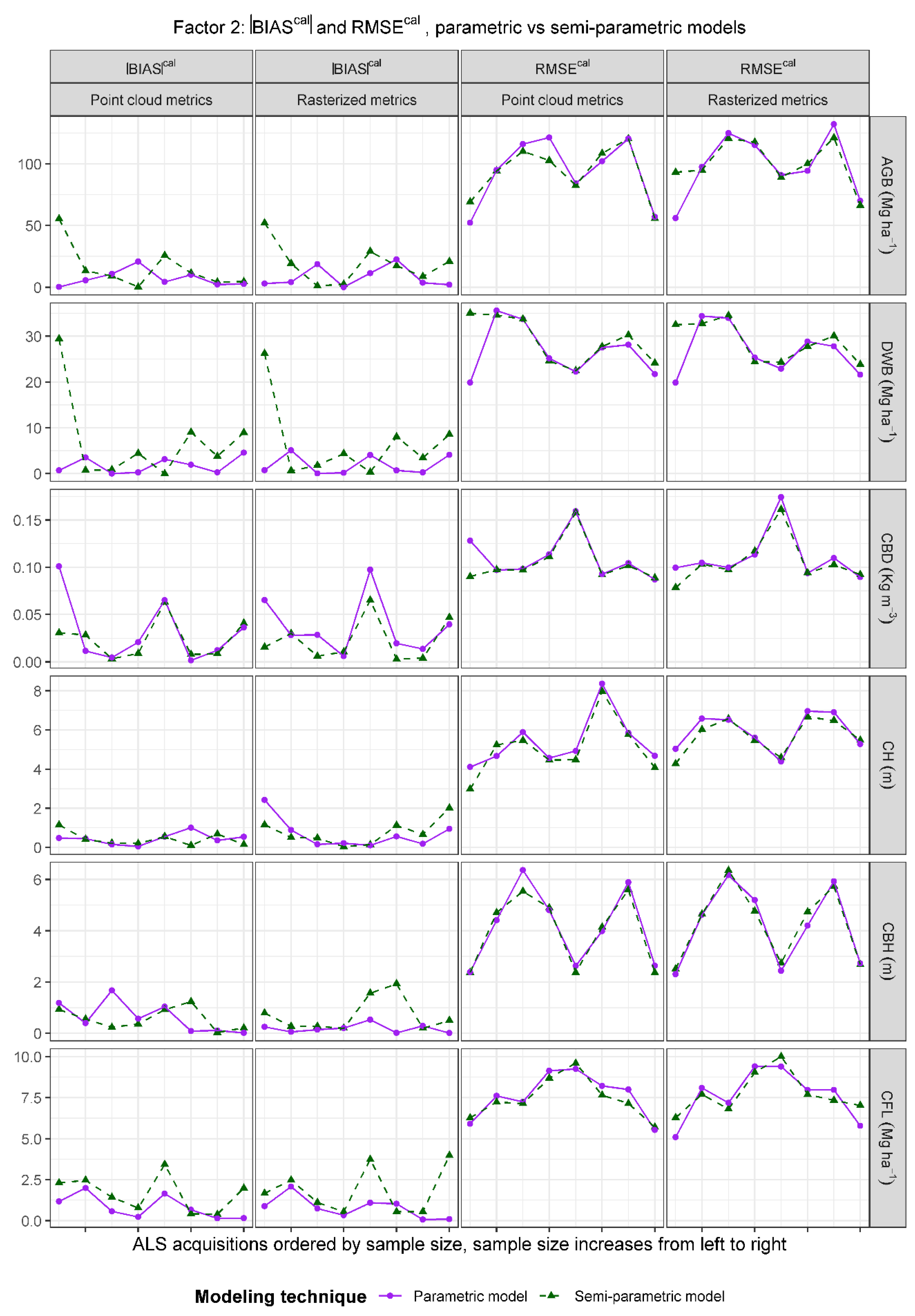
Except for CFL, where parametric models consistently had lower ALS-acquisition-specific values of , differences between parametric and semiparametric models did not show clear patterns of dominance of a modeling technique over the other in terms of (Figure 6). In terms of , semiparametric models provided slightly lower acquisition specific values of for CBD and CH and for the remaining variables no modeling technique consistently provided lower values of this performance metric. For both sources of ALS predictors, the magnitude of the differences between parametric and semiparametric models in was, in general, orders of magnitude smaller than the values of themselves. Similar results were obtained when comparing parametric and semiparametric models with the extended dataset that included 12 additional ALS acquisitions (Figure A4) and only used rasterized predictors. These results show that multiple exceptions to the trends observed for the global and can be observed when focusing on specific ALS acquisitions and confirmed that differences in performance due to the modeling technique are very minor.
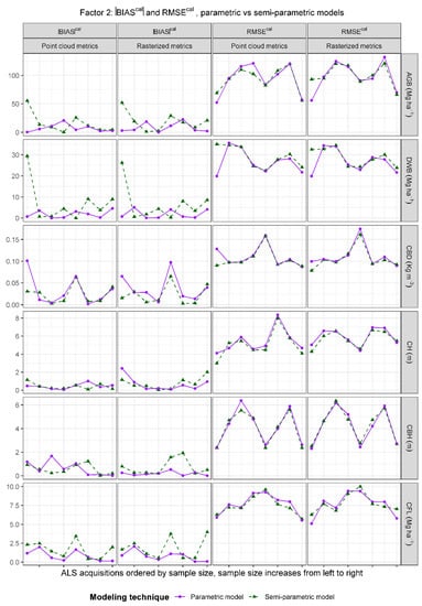
Figure 6.
ALS-acquisition-specific values of absolute bias, , and root mean squared error, , for calibrated predictions for different modeling techniques by ALS data acquisitions. AGB, DWB, CBD, CH, CBH, and CFL respectively indicate aboveground biomass, downed woody biomass, canopy bulk density, canopy height, canopy base height, and canopy fuel load.
3.4. Differences between Sources of ALS Metrics
For the parametric models, differences in global between models based on point-cloud and rasterized ALS predictors were significant only for CBH, and the magnitude of these differences only reached 1.43%. For the semiparametric models, using point-cloud predictors resulted in significantly more accurate models for AGB, CH, CBH, and CFL, but the magnitude of these differences was below 2% for AGB and CH and below 4% and 6% for CBH and CFL respectively. Except for the semiparametric models for DWB, models using point-cloud predictors had lower values of global . However, the magnitude of these differences only reached a 5% for the semiparametric models for CBH, and for the remaining variables differences were always below 3.3% (Table 5).

Table 5.
Differences between models developed using point-cloud metrics and rasterized predictors. AGB, DWB, CBD, CH, CBH, and CFL respectively indicate aboveground biomass, downed woody biomass, canopy bulk density, canopy height, canopy base height, and canopy fuel load. Superscripts and indicate error metrics for models point-cloud and rasterized predictors and the superscript denote changes in and due to using a different source of ALS metrics.
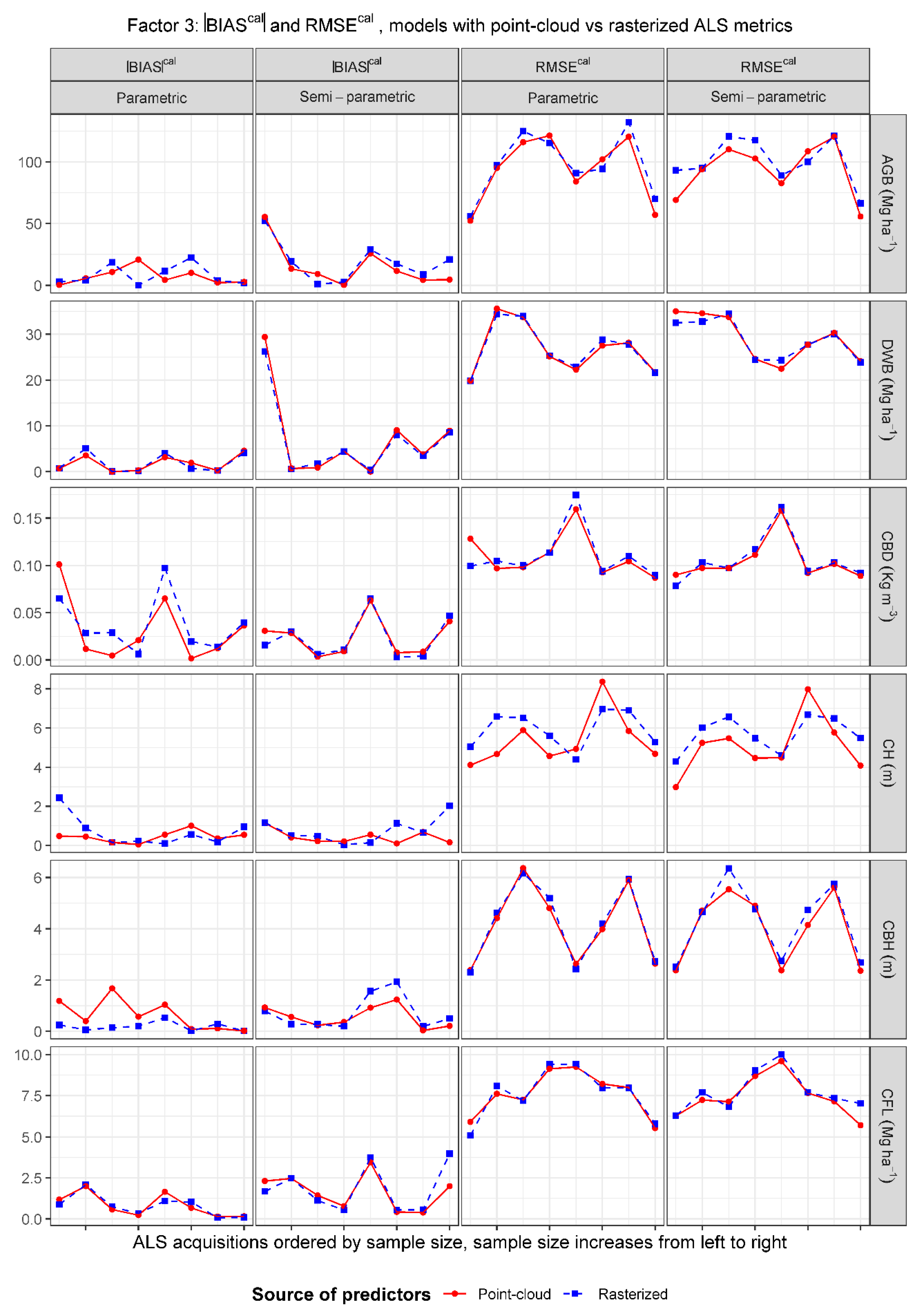
Finally, side by side comparison of ALS-acquisition-specific values of and for models using point-cloud and rasterized metrics showed that models using point-cloud predictors were not always better than the models using rasterized metrics (Figure 7). The only exceptions to this trend were the models for CH in which using point-cloud predictors resulted in about 1 m smaller for most acquisitions. More important, the magnitude of the change in acquisition specific and was generally negligible compared to the values of these metrics. This suggests that using rasterized metrics instead of point-cloud metrics has a limited impact on accuracy.
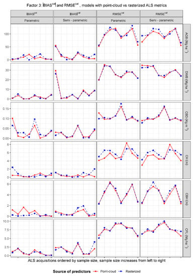
Figure 7.
ALS-acquisition-specific values of absolute bias, , and root mean squared error, , for calibrated predictions for different sources ALS predictors by modeling techniques. AGB, DWB, CBD, CH, CBH, and CFL respectively indicate aboveground biomass, downed woody biomass, canopy bulk density, canopy height, canopy base height, and canopy fuel load.
4. Discussion
We considered the prediction of a wide array of attributes of interest for forest managers and observed important differences between variables. Models for CH and AGB showed a high predictive performance, similar to that found in previous studies [20,26,62,63]. The percentages of explained variance for both parametric and semiparametric models for CBH and CFL were similar to those obtained by [20] for a single ALS acquisition. For CBD the percentage of explained variance of the semiparametric models was about 10% smaller than those reported by [20] for ALS acquisition-specific models. The low values obtained for DWB were also about 10% smaller than those reported by [20] for local models, indicating that regional models developed using the auxiliary information considered in this study only provide a very crude approximation to reality for this variable.
Important efforts have recently been made to analyze the potential transferability of ALS models to new acquisitions not considered in the training dataset [27,28,29] or to a new collection over the same study area [64]. These studies showed that the degradation in model performance due to temporal offsets, and differences in the configuration of the ALS data collection are small compared to the losses in performance due to (1) ecological differences between the regions where the models were fit and transferred, and (2) the effect of the modeling technique. In our study we focused on developing models that can be calibrated to new acquisitions as a way of developing maps of forest fuels and structural attributes in a rapid manner. Our results partially align with those obtained by [29] and for almost all response variables, synthetic predictions from semiparametric models had lower than synthetic predictions from parametric models. The most important effect of the calibration in the parametric models was the reduction in the ALS-acquisition-specific . Such reduction cannot be obtained transferring fixed-effect models to new ALS acquisition as fixed-effect models can only generate synthetic predictions. Once the parametric models were calibrated, few differences were observed between both modeling techniques. One factor that should be considered in future applications is that models developed with more ALS acquisitions will result in more reliable estimates of the variance parameters of the random effects [57]. For cases with fewer ALS acquisitions of large size or where the calibration is not an issue because no new ALS acquisitions are expected, other modeling techniques using only fixed-effects models would be more appropriate. We developed this study using eight ALS acquisitions, but main results were confirmed in the analysis of the extended dataset with 20 ALS acquisitions (Appendix A).
The minor effect that calibration had in the semiparametric models can be explained by the ability of random forest to effectively use large numbers of predictors and model nonlinear patterns [37,38]. If the training dataset covers the main ecological gradients of the area under analysis, random forest captures the most important sources of variability that can be explained by the auxiliary information leaving little room for improvements in the calibration step. The linear mixed-effects models with random intercepts and slopes developed in this study operate in a very different manner. The fixed component of the model characterizes the main relationships between auxiliary information and response variables and complex effects, specific of a given ALS data collection, are accounted for in the calibration step.
Results from our study support the idea that both techniques produce comparable results if calibration is a possibility and suggest the following recommendations for future applications. When calibration is a possibility, linear mixed-effects models do not provide consistently worse results than semiparametric models and have clear advantages in terms of simplicity, interpretability, and ease of use. Apart from the corresponding ground data and auxiliary information, only parameters reported in Table A4 and Table A5 are necessary to develop the calibrations of the parametric linear models. For random forest-based semiparametric models, external users need to have access to the original random forest data-structure developed by the modeler to obtain predictions in new areas. In addition, linear mixed-effects models allow mapping uncertainty of predictions using well-known methods [58,65], but reporting the same uncertainties for semiparametric models is still a field under development [38,66]. When calibration is not a possibility, or a fast and direct model transfer is necessary, semiparametric models are clearly a better option. For these models, synthetic predictions and calibrated predictions showed little differences for all variables, which indicates that omitting the calibration step should not imply significant losses in accuracy with respect to a scenario where calibration is possible.
Regardless of the modelling technique and source of ALS predictors, for all responses analyzed in this study, ALS-acquisition-specific biases did not completely disappear after the calibration step indicating that global models should not be a replacement for ALS-acquisition-specific models, but instead a solution to enable a fast mapping of forest attributes. This result is consistent with [30,31] for nonparametric random forest models. The calibration approach used in this study relies on the assumption of having different error structures due to membership in a particular ALS acquisition. This assumption is reasonable because ALS acquisitions usually cover relatively homogeneous areas and the specifications in the ALS data collection can differ among ALS data-collection projects. The inclusion of ALS-acquisition-specific random effects allows accounting for these differences between ALS acquisitions in the calibration step. Nevertheless, other approaches to calibration should be investigated in the future. Of special interest is the approach proposed by [31] that develops calibrated predictions by considering the variability of geographic areas that do not have to match a specific ALS acquisition.
Differences between models using point-cloud and rasterized metrics were negligible (Figure 7 and Figure A7). Differences of such a small magnitude were not expected; however, this result can be explained by: (1) the presence of GPS positioning errors that even if expected to be in the range of a meter introduce some noise in the ALS metrics [67], and (2) by the averaging that occurs when aggregating point-cloud metrics at the FIA plot level. FIA plots are composed of four 17.95 m radius subplots, with one subplot at the center and the other three subplots 36.58 m from the central plot. Point clouds for the subplots are combined when computing ALS predictors for an FIA plot, resulting in an aggregation effect similar to the one that occurs when computing rasterized metrics. While the use of pre-rasterized layers to e × tract ALS predictors implies a departure from traditional workflows using ALS data, this process is equivalent to that used in many applications using optical sensors such as Landsat images (e.g., [26]) and has been used in previous studies to combine ALS, optical, and topographic predictors [68]. Additionally, and more importantly: (1) ALS metrics are computed in a standardized and structured way that for every point of the territory assigns a unique support area [69] for the computation of ALS metrics, and (2) empirical results from our analysis showed that, by using rasterized ALS metrics instead of point-cloud metrics, the predictive performance of the models does not worsen substantially and allows generating cartographic products useful for multiple planning tasks, with accuracies and precisions similar to those obtained using point-cloud predictors.
The small differences between models developed using point-clouds or rasterized predictors in combination with the fact that sharing rasterized products is far more operationally feasible than sharing large point-clouds, opens the possibility of developing models in a more efficient way. Future mapping applications that require rapid delivery could be developed extracting ALS metrics for the training units using interpolation over pre-rasterized products available from spatial data infrastructures serving raster layers with metrics derived using a standardized workflow. Operating in this way eliminates the need of intersecting ground measurements with large point clouds that are more difficult to share and manipulate, since a larger number of users will be more comfortable extracting auxiliary variables from raster files than clipping and normalizing point-cloud data. These two factors combined can reduce (1) the time needed to develop models and (2) the time that forest managers need to wait for maps of structural attributes once an ALS data are acquired and processed.
5. Conclusions
The increasing availability of ALS data in the western US states raises questions about methodological aspects to derive cartographic products of forest attributes such as AGB, DWB, CBD, CH, CBH, and CFL. This study analyzes three factors of importance for development of a regional strategy to map forest structural attributes that allows using available ALS data acquisitions and incorporating new ALS project areas in a rapid manner. The main conclusion regarding these factors are:
Transferability and calibration. For both modeling techniques, calibration reduced bias problems when predicting to ALS data acquisitions not included in the training dataset; however, the effect of calibration was much more important for parametric linear mixed-effects models than for semiparametric models using random forest. This indicates that linear models developed over such a large region only account for main trends with respect to the auxiliary information and need to (1) account for the variability between ALS data acquisitions and (2) be calibrated to local conditions to eliminate bias problems.
Modeling technique. Once the calibration is performed, both modeling techniques have similar performance in terms of acquisition-specific or . Interpretability of results and simplicity make the linear mixed-effects models more appealing for situations where performing a calibration for new acquisitions is feasible, and the small effect of calibration in semiparametric models makes them a better choice for cases where calibration is not possible.
Source of ALS metrics. Differences in performance between models developed with predictors obtained by interpolation over rasterized ALS metrics and models developed using predictors computed by clipping the point clouds coincident with areas where field measurements were taken were minimal for the variables considered in this study. This clearly suggests that raster layers can be used to drive the entire modeling workflow with little loss in terms of performance, which can be important for time-sensitive applications because the pre-processing of the ALS data can be substantially simplified.
Author Contributions
Conceptualization, F.M., A.T.H., and P.A.F.; methodology, F.M. and A.T.H.; software, F.M.; validation, F.M.; formal analysis, F.M.; investigation, F.M., A.T.H. and P.A.F.; resources, A.T.H., H.T. and D.M.B.; data curation, F.M., P.A.F., and A.T.H.; writing—original draft preparation, F.M.; writing—review and editing, F.M., A.T.H., P.A.F., B.F., H.T., D.M.B., M.J.G., and T.R.M.; visualization, F.M.; supervision, A.T.H.; project administration, A.T.H.; funding acquisition, A.T.H. All authors have read and agreed to the published version of the manuscript.
Funding
This work was funded by the Joint Fire Science Program’s Fire and Smoke Model Evaluation Experiment (Project 15-S-01-01), through a Joint Venture Agreement (17-JV-11221633-185) between the USDA Forest Service Rocky Mountain Research Station and Oregon State University and by the NASA Carbon Monitoring System project: A bottom-up, stakeholder-driven CMS for regional biomass carbon dynamics: Phase II, through a Joint Venture Agreement (20-JV-11221633-112) between the USDA Forest Service Rocky Mountain Research Station and Oregon State University.
Acknowledgments
We would like to thank scientists, technicians, and field crews from the Pacific Northwest FIA program for their efforts in the collecting, compiling, and documenting the ground observations used in this study.
Conflicts of Interest
The authors declare no conflict of interest.
Appendix A. Effect of Calibration and Modeling Technique using Rasterized Predictors and an Extended Set of ALS Acquisitions
An extended dataset was used to assess the factors (1) transferability and effect of calibration and (2) differences between modeling techniques. In this analysis, 12 additional ALS acquisitions were included in the dataset (Figure A1, Table A1 and Table A2). For the extended dataset, 20 ALS acquisitions in total, we analyzed the first two factors: (1) transferability and calibration and (2) modeling technique. The third factor, source of ALS predictors, was omitted for the analysis because for the 12 additional acquisitions point-cloud predictors for the FIA plots were not available at the time of the analysis. Therefore, it was impossible to analyze the effect of the third factor, source of ALS predictors. Means and standard deviation of the variables of interest in the extended dataset are reported in Table A2. For each variable we obtained parametric and semiparametric models using the FIA plots in the combined dataset using the model selection methods described in Section 2.3.1 and Section 2.4.1. Error metrics and model comparisons described in Section 2.5 were computed for the parametric and semiparametric models fitted with the extended dataset.
Selected parametric models are reported in Table A6, and predictors and variance components of the semiparametric models are shown in Figure A6 and Table A8. Models fitted with the extended dataset were very similar to those obtained with the set of eight ALS acquisitions used in the main study and few differences were observed with respect to: (1) global model performance (Figure A2), (2) predictors included in the model, Table A6 and Figure A6, and (3) structure of model errors and random effects (Table A6 and Table A8).
The effect of the calibration was important for the parametric models and negligible for the semiparametric models. The most important effect of calibration in the parametric models was a reduction in the ALS-acquisition-specific (Figure A3). The magnitude of this effect varied among variables from a negligible effect for CBD to substantial reductions in ALS-acquisition-specific for AGB, CBH, and CFL.
Once calibrated, the parametric models had smaller values of global except for AGB and larger values of global s. These results are similar to those obtained with the main dataset and confirm that, globally, parametric models are less prone to bias problems, and semiparametric models tend to have smaller s (Figure A4). Difference in and s for specific ALS acquisitions also showed that trends observed for the global and s have multiple exceptions when observing ALS acquisitions specific performance metrics. ALS-specific and s showed that no modeling technique was consistently better than the other one in terms of these metrics (Figure A4). This result indicates that factors such as model interpretability or the possibility of omitting the calibration are expected to be more relevant than differences in model performance when selecting a modeling technique for a similar problem. Overall, results from this extended analysis confirmed the main conclusions obtained for the factors transferability and effect of calibration and differences between modeling techniques.
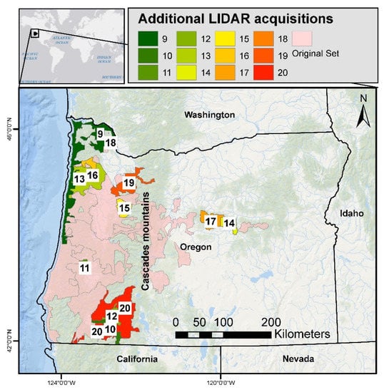
Figure A1.
Predictors included in the semiparametric models and variable importance as percent reduction in mean.
Figure A1.
Predictors included in the semiparametric models and variable importance as percent reduction in mean.
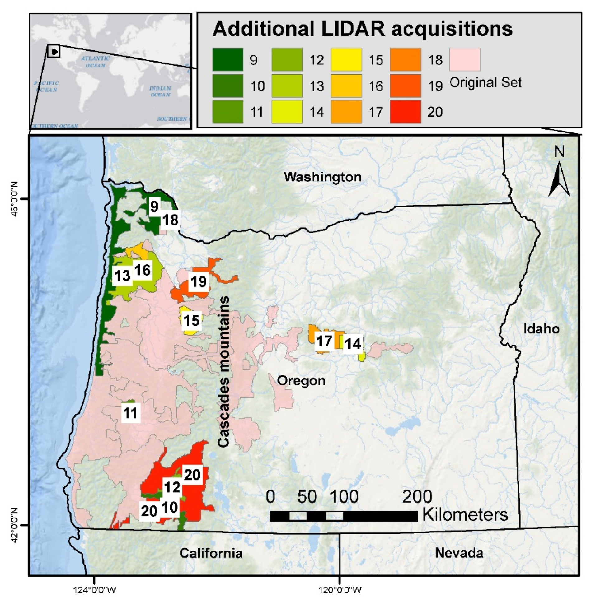

Table A1.
Additional ALS data acquisitions summary and number of field plots per ALS acquisition. * Data collection date not reported by vendor; flying altitude and sensor inferred from the data reported for acquisitions obtained the same year.
Table A1.
Additional ALS data acquisitions summary and number of field plots per ALS acquisition. * Data collection date not reported by vendor; flying altitude and sensor inferred from the data reported for acquisitions obtained the same year.
| ALS Data Acquisition | End Year | Flying Altitude (m) | Sensor | Average Pulse Density (Pulses/m2) | Area (Km2) | FIA PLOTS |
|---|---|---|---|---|---|---|
| 9. North Coast | 2009 | 900 * | Leica ALS50 PII* | 8.00 | 4506.55 | 77 |
| 10. Medford | 2009 | 900 * | Leica ALS50 PII* | 7.80 | 984.5 | 14 |
| 11. Umpqua | 2008 | 900 | Leica ALS50 PII | 8.80 | 272.92 | 6 |
| 12. Eagle Point | 2010 | 900 | Leica ALS60 | 8.08 | 546.58 | 7 |
| 13. Yambo | 2010 | 900–1300 | Leica ALS50 and ALS60 | 9.17 | 2803.88 | 69 |
| 14. Ochoco A | 2011 | 1300 | Leica ALS50 | 9.74 | 795 | 57 |
| 15. Green Peter | 2012 | 900 | Leica ALS60 | 9.81 | 897.71 | 25 |
| 16. Tillamook Yamhill | 2012 | 900 | Leica ALS50 and ALS60 | 9.72 | 808.72 | 16 |
| 17. Ochoco B | 2013 | 900 | Leica ALS60 | 9.07 | 1228.71 | 39 |
| 18. Scapoose | 2013 | 900 | Leica ALS60 | 7.60 | 150.64 | 3 |
| 19. Clackamol | 2013 | 900 | Leica ALS60 | 9.19 | 1835.42 | 40 |
| 20. Upper Rogue | 2015 | 1200–1500 | Optech Orion H, LeicaALS 70 and ALS80 | 12.24 | 5654.01 | 166 |
| Additional plots | 20,548.66 | 519 | ||||
| Total dataset (Including acquisitions 1–8) | 66,695.17 | 1652 | ||||

Table A2.
Means and standard deviations of the variables of interest in the extended dataset.
Table A2.
Means and standard deviations of the variables of interest in the extended dataset.
| FIA PLOTS | Mean (Standard Deviation) of Response Variables | ||||||
|---|---|---|---|---|---|---|---|
| AGB (Mg/ha) | DWB (Mg/ha) | CBD (Kg/m3) | CH (m) | CBH (m) | CFL (Mg/ha) | ||
| All acquisitions | 1652 | 236.26 | 27.7 | 0.14 | 31.11 | 4.97 | 15.51 |
| (206.52) | (28.82) | (0.12) | (15.31) | (5.26) | (10.99) | ||

Figure A2.
Relative root mean squared error (RRMSEcal), relative bias (RBIAScal), and coefficient of determination (R2) for parametric and semiparametric models using rasterized predictors in the extended dataset of 20 ALS acquisitions. Model response variables are: aboveground biomass (AGB), downed woody biomass (DWB), canopy bulk density (CBD), canopy height (CH), canopy base height (CBH), and canopy fuel loading (CFL).
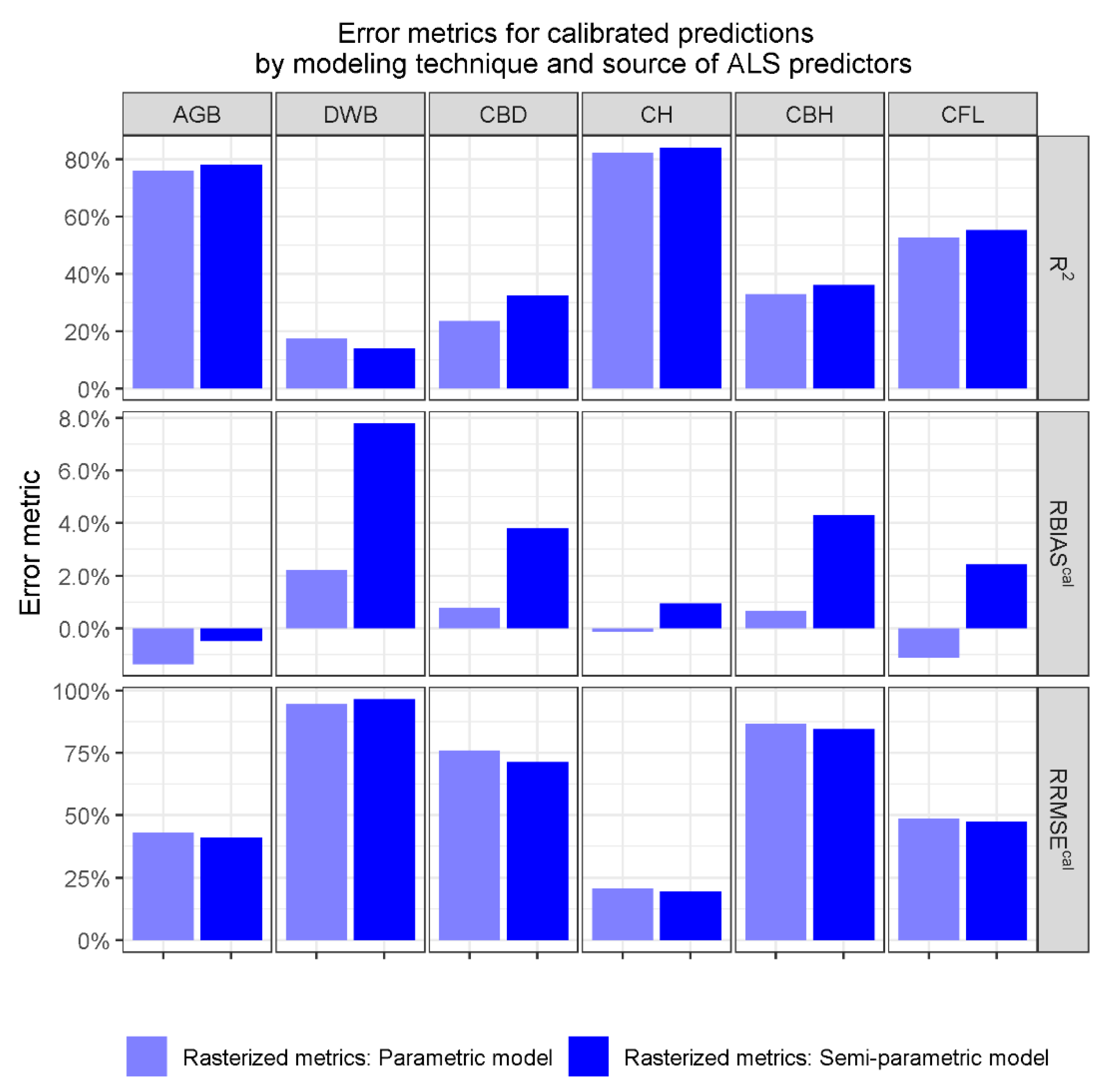

Table A3.
Global differences between parametric and semiparametric models in the extended dataset of 20 ALS acquisitions. AGB, DWB, CBD, CH, CBH, and CFL respectively indicate aboveground biomass, downed woody biomass, canopy bulk density, canopy height, canopy base height, and canopy fuel load. Superscripts and indicate error metrics for parametric and semiparametric models respectively and the superscript denote changes in and due to using a different modeling technique.
| Variable | Set of Acquisitions & Source of ALS Metrics | t-Test Accuracy | t-Test Magnitude | ∆RBIASm | ∆RRMSEm | ||
|---|---|---|---|---|---|---|---|
| Mean Difference | p-Value | Mean Difference | p-Value | ||||
| AGB (Mg/ha) | Extended set raster | −2.05 | 6.41 × 10⁻² | 4.25 | 1.36 × 10⁻⁵ | 0.87% | 1.94% |
| DWB (Mg/ha) | Extended set-raster | −1.54 | 7.90 × 10⁻⁹ | −3.84 × 10⁻¹ | 1.12 × 10⁻¹ | −5.57% | −1.96% |
| CBD (Kg/m3) | Extended set-raster | −4.27 × 10⁻³ | 3.49 × 10⁻⁵ | 2.40 × 10⁻³ | 1.24 × 10⁻² | −3.01% | 4.56% |
| CH (m) | Extended set-raster | −3.40 × 10⁻¹ | 3.29 × 10⁻⁶ | 7.87 × 10⁻² | 2.42 × 10⁻¹ | −0.80% | 1.03% |
| CBH(m) | Extended set-raster | −1.81 × 10⁻¹ | 7.55 × 10⁻⁵ | 7.14 × 10⁻² | 9.20 × 10⁻² | −3.63% | 2.15% |
| CFL (Mg/ha) | Extended set-raster | −5.50 × 10⁻¹ | 5.25 × 10⁻¹³ | 9.35 × 10⁻² | 1.48 × 10⁻¹ | −1.30% | 1.39% |
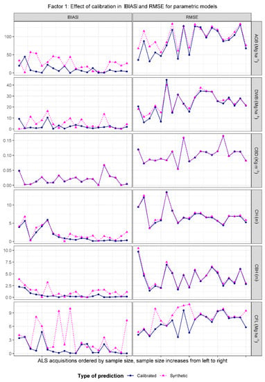
Figure A3.
ALS-acquisition-specific and for synthetic and calibrated predictions for parametric and models. AGB, DWB, CBD, CH, CBH and CFL respectively indicate aboveground biomass, downed woody biomass, canopy bulk density, canopy height, canopy base height, and canopy fuel load.
Figure A3.
ALS-acquisition-specific and for synthetic and calibrated predictions for parametric and models. AGB, DWB, CBD, CH, CBH and CFL respectively indicate aboveground biomass, downed woody biomass, canopy bulk density, canopy height, canopy base height, and canopy fuel load.
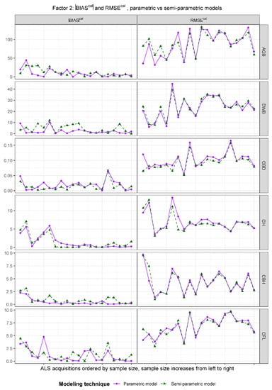
Figure A4.
ALS-acquisition-specific values of absolute relative bias, , and relative root mean squared error, , for synthetic and calibrated predictions for parametric and models. AGB, DWB, CBD, CH, CBH and CFL respectively indicate aboveground biomass, downed woody biomass, canopy bulk density, canopy height, canopy base height, and canopy fuel load.
Appendix B. Selected Parametric and Semiparametric Models

Table A4.
Parameters and global performance metrics of linear mixed-effects models using point-cloud ALS predictors. * Indicates the most correlated predictor used to model heteroscedasticity. Model response variables are: aboveground biomass (AGB), downed woody biomass (DWB), canopy bulk density (CBD), canopy height (CH), canopy base height (CBH), and canopy fuel loading (CFL).
| Variable | Fixed-Effect Parameters | Error Variance | Random Effects | RMSEcal | Biascal | |||||||
|---|---|---|---|---|---|---|---|---|---|---|---|---|
| Coefficient | Value | p-Value | σe | α | Var(v)0.5 | Correlation Matrix of v | ||||||
| AGB (Mg/ha) | (Intercept) | 3.20 × 101 | 9.60 × 10⁻⁶ | 2.02 × 10² | 2.62 × 10⁻¹ | 1.58 × 101 | 1.00 | −0.94 | 0.59 | −0.75 | 9.59 × 101 | −3.88 |
| % Returns [16 m, 32 m) | 3.80 × 10² | 4.90 × 10⁻¹⁶ | 1.19 × 10² | −0.94 | 1.00 | −0.39 | 0.85 | |||||
| % Returns [32 m, 48 m) * | 7.30 × 10² | 1.20 × 10⁻³¹ | 1.12 × 10² | 0.59 | −0.39 | 1.00 | −0.54 | |||||
| % Returns [48 m, 64 m) | 1.80 × 10³ | 3.30 × 10⁻¹⁰ | 6.94 × 10² | −0.75 | 0.85 | −0.54 | 1.00 | |||||
| DWB (Mg/ha) | (Intercept) | 2.40 × 101 | 6.80 × 10⁻¹⁷ | 1.12 × 101 | 1.89 × 10⁻¹ | 1.83 | 1.00 | 0.11 | 0.05 | 2.65 × 101 | 2.20 | |
| sdi | −2.60 | 1.60 × 10⁻⁷ | 8.00 × 10⁻¹ | 0.11 | 1.00 | −0.99 | ||||||
| P95 * | 1.80 × 10⁻¹ | 2.60 × 10⁻¹⁵ | 3.20 × 10⁻² | 0.05 | −0.99 | 1.00 | ||||||
| CBD (Kg/m3) | (Intercept) | −1.30 × 10⁻² | 4.60 × 10⁻¹ | 8.10 × 10⁻² | 5.00 × 10⁻² | 3.15 × 10⁻² | 1.00 | −0.98 | −0.49 | −0.08 | 1.06 × 10⁻¹ | 1.05 × 10⁻² |
| %First returns above 2 m * | 2.50 × 10⁻³ | 2.40 × 10⁻³⁴ | 3.53 × 10⁻⁴ | −0.98 | 1.00 | 0.63 | −0.09 | |||||
| StdDev | −2.70 × 10⁻³ | 3.90 × 10⁻²⁵ | 1.99 × 10⁻⁴ | −0.49 | 0.63 | 1.00 | −0.83 | |||||
| ×10lev | 8.90 × 10⁻⁵ | 3.00 × 10⁻⁵ | 5.22 × 10⁻⁵ | −0.08 | −0.09 | −0.83 | 1.00 | |||||
| CH (m) | (Intercept) | 2.00 | 2.10 × 10⁻⁶ | 3.50 | 1.04 × 10⁻¹ | 2.58 × 10⁻¹ | 1.00 | −1.00 | 5.58 | 3.97 × 10⁻² | ||
| P95 * | 3.00 × 10⁻¹ | 4.50 × 10−252 | 1.46 × 10⁻² | −1.00 | 1.00 | |||||||
| CBH (m) | (Intercept) | 6.60 × 10⁻¹ | 1.10 × 10⁻¹ | 4.67 × 10⁻¹ | 5.32 × 10⁻¹ | 4.31 × 10⁻¹ | 1.00 | 0.90 | −0.20 | −0.83 | 4.36 | −4.78 × 10⁻² |
| CRR | 7.30 | 5.80 × 10⁻⁸ | 1.24 | 0.90 | 1.00 | −0.60 | −0.99 | |||||
| P50 * | 5.20 × 10⁻² | 1.70 × 10⁻¹³ | 9.06 × 10⁻³ | −0.20 | −0.60 | 1.00 | 0.72 | |||||
| ×10lev | −1.60 × 10⁻³ | 3.90 × 10⁻⁶ | 5.75 × 10⁻⁴ | −0.83 | −0.99 | 0.72 | 1.00 | |||||
| CFL (Mg/ha) | (Intercept) | −1.10 × 101 | 3.40 × 10⁻¹¹ | 7.43 | 3.44 | 1.00 | 0.30 | −0.99 | 0.80 | 7.53 | −1.40 × 10⁻¹ | |
| P05 | 1.80 × 10⁻¹ | 1.10 × 10⁻⁹ | 3.40 × 10⁻² | 0.30 | 1.00 | −0.40 | 0.81 | |||||
| %First returns above 2 m | 2.60 × 10⁻¹ | 1.20 × 10⁻²⁴ | 6.04 × 10⁻² | −0.99 | −0.40 | 1.00 | −0.86 | |||||
| ×10lev | 9.70 × 10⁻³ | 1.80 × 10⁻⁹ | 3.98 × 10⁻³ | 0.80 | 0.81 | −0.86 | 1.00 | |||||

Table A5.
Parameters and global performance metrics of linear mixed-effects models using rasterized ALS predictors. * Indicates the most correlated predictor used to model heteroscedasticity. Model response variables are: aboveground biomass (AGB), downed woody biomass (DWB), canopy bulk density (CBD), canopy height (CH), canopy base height (CBH), and canopy fuel loading (CFL).
| Variable | Fixed-Effect Parameters | Error Variance | Random Effects | RMSEcal | Biascal | ||||||||
|---|---|---|---|---|---|---|---|---|---|---|---|---|---|
| Coefficient | Value | p-Value | σe | α | Var(v)0.5 | Correlation Matrix of v | |||||||
| AGB (Mg/ha) | (Intercept) | 3.10 × 101 | 2.50 × 10⁻¹ | 3.78 × 101 | 3.30 × 10⁻¹ | 6.80 × 101 | 1.00 | −0.99 | 0.76 | −0.63 | 1.02 × 10² | −9.64 × 10⁻² | |
| CRR | −3.30 × 10² | 2.40 × 10⁻⁶ | 1.66 × 10² | −0.99 | 1.00 | −0.80 | 0.66 | ||||||
| Mean * | 1.80 × 101 | 4.00 × 10⁻³⁴ | 3.63 | 0.76 | −0.80 | 1.00 | −0.96 | ||||||
| %First returns above 2 m | 5.90 × 10⁻¹ | 2.50 × 10⁻² | 6.44 × 10⁻¹ | −0.63 | 0.66 | −0.96 | 1.00 | ||||||
| DWB (Mg/ha) | (Intercept) | 2.50 × 101 | 3.90 × 10⁻¹⁶ | 1.52 × 101 | 1.68 × 10⁻¹ | 3.77 | 1.00 | 0.58 | −0.69 | 2.66 × 101 | 2.11 | ||
| sdi | −2.60 | 4.50 × 10⁻⁸ | 7.32 × 10⁻¹ | 0.58 | 1.00 | −0.99 | |||||||
| P95 * | 5.60 × 10⁻¹ | 2.80 × 10⁻¹⁰ | 1.72 × 10⁻¹ | −0.69 | −0.99 | 1.00 | |||||||
| CBD (Kg/m3) | (Intercept) | 1.30 × 10⁻¹ | 9.80 × 10⁻² | 6.46 × 10⁻² | 1.06 × 10⁻¹ | 1.67 × 10⁻¹ | 1.00 | −0.95 | −0.52 | −0.08 | 0.15 | 1.10 × 10⁻¹ | 1.15 × 10⁻² |
| mmax | −8.50 × 10⁻³ | 2.00 × 10⁻³ | 5.87 × 10⁻³ | −0.95 | 1.00 | 0.24 | −0.14 | 0.15 | |||||
| sday | 1.00 × 10⁻³ | 2.10 × 10⁻⁴ | 5.78 × 10⁻⁴ | −0.52 | 0.24 | 1.00 | 0.50 | −0.91 | |||||
| %First returns above 2 m * | 2.20 × 10⁻³ | 1.80 × 10⁻²⁴ | 4.29 × 10⁻⁴ | −0.08 | −0.14 | 0.50 | 1.00 | −0.43 | |||||
| StdDev | −8.70 × 10⁻³ | 3.10 × 10⁻¹⁷ | 1.43 × 10⁻³ | 0.15 | 0.15 | −0.91 | −0.43 | 1.00 | |||||
| CH (m) | (Intercept) | 5.00 | 2.30 × 10⁻³⁰ | 5.98 | 3.37 × 10⁻² | 1.00 | 0.99 | 6.01 | 2.36 × 10⁻¹ | ||||
| P95 | 9.50 × 10⁻¹ | 4.10 × 10−215 | 5.25 × 10⁻² | 0.99 | 1.00 | ||||||||
| CBH (m) | (Intercept) | 2.30 | 9.50 × 10⁻³ | 5.63 | 3.18 × 10⁻¹ | 1.66 | 1.00 | −0.52 | −0.98 | −0.32 | 4.44 | 1.19 × 10⁻¹ | |
| CRR * | 1.30 × 101 | 1.60 × 10⁻¹⁵ | 3.29 | −0.52 | 1.00 | 0.31 | −0.65 | ||||||
| % Returns [8 m,16 m) | −7.30 | 5.40 × 10⁻¹¹ | 1.58 | −0.98 | 0.31 | 1.00 | 0.52 | ||||||
| Elev | −2.60 × 10⁻³ | 1.70 × 10⁻⁵ | 1.39 × 10⁻³ | −0.32 | −0.65 | 0.52 | 1.00 | ||||||
| CFL (Mg/ha) | (Intercept) | −8.50 | 2.10 × 10⁻⁸ | 7.52 | 3.06 | 1.00 | 0.42 | −0.99 | 0.77 | 7.63 | −8.23 × 10⁻² | ||
| P05 | 4.10 × 10⁻¹ | 4.90 × 10⁻⁹ | 1.21 × 10⁻¹ | 0.42 | 1.00 | −0.52 | 0.88 | ||||||
| %First returns above 2 m | 2.20 × 10⁻¹ | 6.60 × 10⁻²² | 5.41 × 10⁻² | −0.99 | −0.52 | 1.00 | −0.84 | ||||||
| Elev | 9.70 × 10⁻³ | 3.10 × 10⁻¹⁰ | 3.75 × 10⁻³ | 0.77 | 0.88 | −0.84 | 1.00 | ||||||

Table A6.
Parameters and global performance metrics of linear mixed-effects models using rasterized predictors on extended set of 20 ALS data acquisitions with rasterized metrics described in Appendix A. * Indicates the most correlated predictor used to model heteroscedasticity. Model response variables are: aboveground biomass (AGB), downed woody biomass (DWB), canopy bulk density (CBD), canopy height (CH), canopy base height (CBH), and canopy fuel loading (CFL).
| Variable | Fixed-Effect Parameters | Error Variance | Random Effects | RMSEcal | Biascal | |||||||
|---|---|---|---|---|---|---|---|---|---|---|---|---|
| Coefficient | Value | p-Value | σe | α | Var(v)0.5 | Correlation Matrix of v | ||||||
| AGB (Mg/ha) | (Intercept) | 4.80 × 101 | 3.70 × 10⁻² | 3.83 × 101 | 3.33 × 10⁻¹ | 8.69 × 101 | 1.00 | −0.99 | 0.73 | −0.73 | 1.01 × 10² | −3.23 |
| CRR | −3.50 × 10² | 8.30 × 10⁻¹¹ | 1.81 × 10² | −0.99 | 1.00 | −0.79 | 0.77 | |||||
| Mean * | 1.80 × 101 | 9.70 × 10−45 | 4.67 | 0.73 | −0.79 | 1.00 | −0.96 | |||||
| %First returns above Mean | 1.10 | 1.60 × 10⁻² | 1.64 | −0.73 | 0.77 | −0.96 | 1.00 | |||||
| DWB (Mg/ha) | (Intercept) | 2.40 × 101 | 1.70 × 10⁻¹¹ | 1.28 × 101 | 2.13 × 10⁻¹ | 1.11 × 101 | 1.00 | −0.84 | 0.33 | 2.62 × 101 | 6.15 × 10⁻¹ | |
| sdi | −3.10 | 1.50 × 10⁻⁵ | 2.61 | −0.84 | 1.00 | −0.79 | ||||||
| P95 * | 6.50 × 10⁻¹ | 1.00 × 10⁻¹⁹ | 2.03 × 10⁻¹ | 0.33 | −0.79 | 1.00 | ||||||
| CBD (Kg/m3) | (Intercept) | 5.90 × 10⁻² | 1.30 × 10⁻⁶ | 5.49 × 10⁻² | 1.54 × 10⁻¹ | 3.84 × 10⁻² | 1.00 | −0.94 | 0.22 | 1.08 × 10⁻¹ | 1.11 × 10⁻³ | |
| %First returns above Mean * | 2.10 × 10⁻³ | 1.60 × 10⁻²⁸ | 5.91 × 10⁻⁴ | −0.94 | 1.00 | 0.12 | ||||||
| StdDev | −8.80 × 10⁻³ | 1.30 × 10⁻²⁷ | 8.55 × 10⁻⁴ | 0.22 | 0.12 | 1.00 | ||||||
| CH (m) | (Intercept) | 5.60 | 2.30 × 10⁻²⁰ | 6.39 | 1.70 | 1.00 | −0.60 | 6.42 | −4.61 × 10⁻² | |||
| P95 | 9.40 × 10⁻¹ | 2.80 × 10−265 | 6.44 × 10⁻² | −0.60 | 1.00 | |||||||
| CBH (m) | (Intercept) | 3.70 | 7.30 × 10⁻¹⁵ | 2.32 | 2.45 × 10⁻¹ | 1.40 | 1.00 | −0.14 | −0.91 | 4.30 | 3.33 × 10⁻² | |
| P25* | 2.60 × 10⁻¹ | 2.90 × 10−40 | 4.27 × 10⁻² | −0.14 | 1.00 | −0.03 | ||||||
| ELEV | −2.20 × 10⁻³ | 5.20 × 10⁻¹⁰ | 9.25 × 10⁻⁴ | −0.91 | −0.03 | 1.00 | ||||||
| CFL (Mg/ha) | (Intercept) | −6.20 | 7.00 × 10⁻⁸ | 7.49 | 3.15 | 1.00 | 0.33 | −0.93 | 0.25 | 7.55 | −1.74 × 10⁻¹ | |
| P05 | 4.40 × 10⁻¹ | 3.10 × 10⁻¹⁶ | 9.89 × 10⁻² | 0.33 | 1.00 | −0.30 | 0.24 | |||||
| %First returns above 2 m | 2.00 × 10⁻¹ | 1.60 × 10⁻³⁴ | 5.20 × 10⁻² | −0.93 | −0.30 | 1.00 | −0.57 | |||||
| Elev | 8.10 × 10⁻³ | 5.80 × 10⁻¹⁰ | 4.51 × 10⁻³ | 0.25 | 0.24 | −0.57 | 1.00 | |||||
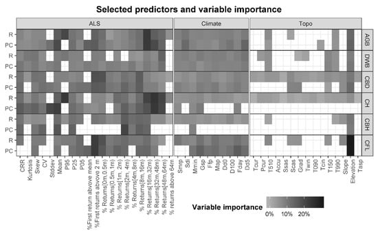
Figure A5.
Predictors included in the semiparametric models and variable importance as percent reduction in mean squared error. R and PC indicate models developed with rasterized and point-cloud metrics respectively. Model response variables are: aboveground biomass (AGB), downed woody biomass (DWB), canopy bulk density (CBD), canopy height (CH), canopy base height (CBH), and canopy fuel loading (CFL).

Table A7.
Variance parameters for the random effects and model errors for the semiparametric models obtained for each response variable, set of ALS acquisition and source of ALS predictors. Model response variables are: aboveground biomass (AGB), downed woody biomass (DWB), canopy bulk density (CBD), canopy height (CH), canopy base height (CBH), and canopy fuel loading (CFL).
| Variable | Source of ALS Predictors | κ | RMSEcal | Biascal | ||
|---|---|---|---|---|---|---|
| AGB (Mg/ha) | Point-cloud | 6.84 | 9.54 × 10⁻¹⁰ | 4.63 × 10⁻¹ | 9.36 × 101 | 1.33 |
| Rasterized | 7.59 | 7.14 × 10⁻¹¹ | 4.54 × 10⁻¹ | 9.84 × 101 | −5.41 | |
| DWB (Mg/ha) | Point-cloud | 2.33 | 7.04 × 10⁻⁶ | 7.15 × 10⁻¹ | 2.76 × 101 | −5.23 |
| Rasterized | 2.20 | 6.33 × 10⁻⁶ | 7.27 × 10⁻¹ | 2.76 × 101 | −4.77 | |
| CBD (Kg/m3) | Point-cloud | 3.73 × 10⁻¹ | 4.98 × 10⁻² | 7.06 × 10⁻¹ | 1.05 × 10⁻¹ | −1.22 × 10⁻² |
| Rasterized | 3.47 × 10⁻¹ | 6.21 × 10⁻² | 6.52 × 10⁻¹ | 1.08 × 10⁻¹ | −1.27 × 10⁻² | |
| CH (m) | Point-cloud | 2.01 | 9.20 × 10⁻¹⁰ | 2.84 × 10⁻¹ | 5.29 | 6.15 × 10⁻² |
| Rasterized | 4.07 | 5.21 × 10⁻¹⁰ | 9.85 × 10⁻² | 5.89 | −5.61 × 10⁻¹ | |
| CH (m) | Point-cloud | 9.52 × 10⁻¹ | 2.60 × 10⁻⁷ | 8.24 × 10⁻¹ | 4.17 | −1.90 × 10⁻¹ |
| Rasterized | 1.25 | 3.03 × 10⁻⁷ | 7.12 × 10⁻¹ | 4.44 | −4.73 × 10⁻¹ | |
| CFL (Mg/ha) | Point-cloud | 1.89 | 1.69 × 10⁻¹³ | 4.75 × 10⁻¹ | 7.29 | −5.40 × 10⁻¹ |
| Rasterized | 1.91 | 3.22 × 10⁻¹³ | 4.86 × 10⁻¹ | 7.78 | −1.01 |
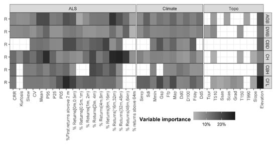
Figure A6.
Predictors included in the semiparametric models and variable importance as percent reduction in mean squared error for the extended set of 20 ALS acquisitions using rasterized predictors described in Appendix A. Model response variables are: aboveground biomass (AGB), downed woody biomass (DWB), canopy bulk density (CBD), canopy height (CH), canopy base height (CBH), and canopy fuel loading (CFL).

Table A8.
Variance parameters for the random effects and model errors for the semiparametric models obtained for each response variable for the extended set of 20 ALS acquisitions using rasterized predictors described in Appendix A. Model response variables are: aboveground biomass (AGB), downed woody biomass (DWB), canopy bulk density (CBD), canopy height (CH), canopy base height (CBH), and canopy fuel loading (CFL).
| Variable | Set of ALS Acquisitions and Source of ALs Predictors | κ | RMSEcal | Biascal | ||
|---|---|---|---|---|---|---|
| AGB (Mg/ha) | Extended set Rasterized | 3.56 | 2.61 × 10⁻² | 5.95 × 10⁻¹ | 9.67 × 101 | 1.18 |
| DWB (Mg/ha) | Extended set Rasterized | 2.23 | 6.81 × 10⁻⁴ | 7.22 × 10⁻¹ | 2.67 × 101 | −2.16 |
| CBD (Kg/m3) | Extended set Rasterized | 3.45 × 10⁻¹ | 6.31 × 10⁻² | 6.63 × 10⁻¹ | 1.01 × 10⁻¹ | −5.38 × 10⁻³ |
| CH (m) | Extended set Rasterized | 5.94 | 4.65 × 10⁻³ | 0.00 | 6.10 | −2.94 × 10⁻¹ |
| CBH(m) | Extended set Rasterized | 1.30 | 4.91 × 10⁻⁷ | 6.76 × 10⁻¹ | 4.20 | −2.14 × 10⁻¹ |
| CFL (Mg/ha) | Extended set Rasterized | 1.80 | 3.06 × 10⁻⁶ | 5.04 × 10⁻¹ | 7.34 | −3.76 × 10⁻¹ |
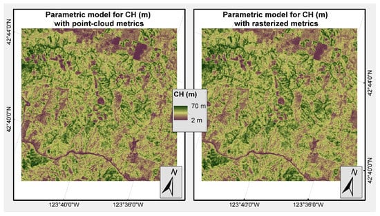
Figure A7.
Maps of canopy height, CH, for a section of the ALS acquisition 5 Rogue Valley. The left map was derived with the parametric model using point-cloud predictors and the right map was obtained with the parametric model using rasterized predictors. Both maps were obtained using the eight ALS acquisitions described in the Section 2.1.
References
- Sing, L.; Metzger, M.J.; Paterson, J.S.; Ray, D. A Review of the Effects of Forest Management Intensity on Ecosystem Services for Northern European Temperate Forests with a Focus on the UK. For. Int. J. For. Res. 2017, 91, 151–164. [Google Scholar] [CrossRef]
- Dunn, C.J.; Thompson, M.P.; Calkin, D.E. A Framework for Developing Safe and Effective Large-Fire Response in a New Fire Management Paradigm. For. Ecol. Manag. 2017, 404, 184–196. [Google Scholar] [CrossRef]
- Kangas, A. Value of Forest Information. Eur. J. For. Res. 2010, 129, 863–874. [Google Scholar] [CrossRef]
- Kangas, A.; Gobakken, T.; Puliti, S.; Hauglin, M.; Naesset, E. Value of Airborne Laser Scanning and Digital Aerial Photogrammetry Data in Forest Decision Making. Silva Fenn. 2018, 52. [Google Scholar] [CrossRef]
- McCarley, T.R.; Hudak, A.T.; Sparks, A.M.; Vaillant, N.M.; Meddens, A.J.H.; Trader, L.; Mauro, F.; Kreitler, J.; Boschetti, L. Estimating Wildfire Fuel Consumption with Multitemporal Airborne Laser Scanning Data and Demonstrating Linkage with MODIS-Derived Fire Radiative Energy. Remote Sens. Environ. 2020, 251, 112114. [Google Scholar] [CrossRef]
- Bechtold, W.A.; Patterson, P.L. The Enhanced Forest Inventory and Analysis Program: National Sampling Design and Estimation Procedures; US Department of Agriculture Forest Service, Southern Research Station Asheville, North Carolina: Asheville, NC, USA, 2005; p. 85.
- Palmer, M.; Christensen, G.; Kuegler, O.; Chase, J.; Fried, J.; Jovan, S.; Mercer, K.; Gray, D.; Loreno, S.; Morgan, T. Oregon’s Forest Resources, 2006–2015: Ten-Year Forest Inventory and Analysis Report; U.S. Department of Agriculture, Forest Service, Pacific Northwest Research Station: Portland, OR, USA, 2018.
- Næsset, E. Predicting Forest Stand Characteristics with Airborne Scanning Laser Using a Practical Two-Stage Procedure and Field Data. Remote Sens. Environ. 2002, 80, 88–99. [Google Scholar] [CrossRef]
- Hudak, A.T.; Strand, E.K.; Vierling, L.A.; Byrne, J.C.; Eitel, J.U.; Martinuzzi, S.; Falkowski, M.J. Quantifying Aboveground Forest Carbon Pools and Flu × es from Repeat LiDAR Surveys. Remote Sens. Environ. 2012, 123, 25–40. [Google Scholar] [CrossRef]
- Valbuena, R.; Maltamo, M.; Martín-Fernández, S.; Packalen, P.; Pascual, C.; Nabuurs, G.-J. Patterns of Covariance between Airborne Laser Scanning Metrics and Lorenz Curve Descriptors of Tree Size Inequality. Can. J. Remote Sens. 2013, 39, S18–S31. [Google Scholar] [CrossRef]
- Huete, A.R.; Liu, H.Q.; Batchily, K.; van Leeuwen, W. A Comparison of Vegetation Indices over a Global Set of TM Images for EOS-MODIS. Remote Sens. Environ. 1997, 59, 440–451. [Google Scholar] [CrossRef]
- Steininger, M.K. Satellite Estimation of Tropical Secondary Forest Above-Ground Biomass: Data from Brazil and Bolivia. Int. J. Remote Sens. 2000, 21, 1139–1157. [Google Scholar] [CrossRef]
- Dong, J.; Kaufmann, R.K.; Myneni, R.B.; Tucker, C.J.; Kauppi, P.E.; Liski, J.; Buermann, W.; Ale × eyev, V.; Hughes, M.K. Remote Sensing Estimates of Boreal and Temperate Forest Woody Biomass: Carbon Pools, Sources, and Sinks. Remote Sens. Environ. 2003, 84, 393–410. [Google Scholar] [CrossRef]
- Avitabile, V.; Baccini, A.; Friedl, M.A.; Schmullius, C. Capabilities and Limitations of Landsat and Land Cover Data for Aboveground Woody Biomass Estimation of Uganda. Remote Sens. Environ. 2012, 117, 366–380. [Google Scholar] [CrossRef]
- Zhang, G.; Ganguly, S.; Nemani, R.R.; White, M.A.; Milesi, C.; Hashimoto, H.; Wang, W.; Saatchi, S.; Yu, Y.; Myneni, R.B. Estimation of Forest Aboveground Biomass in California Using Canopy Height and Leaf Area Index Estimated from Satellite Data. Remote Sens. Environ. 2014, 151, 44–56. [Google Scholar] [CrossRef]
- Zhu, X.; Liu, D. Improving Forest Aboveground Biomass Estimation Using Seasonal Landsat NDVI Time-Series. ISPRS J. Photogramm. Remote Sens. 2015, 102, 222–231. [Google Scholar] [CrossRef]
- Durante, P.; Martín-Alcón, S.; Gil-Tena, A.; Algeet, N.; Tomé, J.L.; Recuero, L.; Palacios-Orueta, A.; Oyonarte, C. Improving Aboveground Forest Biomass Maps: From High-Resolution to National Scale. Remote Sens. 2019, 11, 795. [Google Scholar] [CrossRef]
- Rollins, M.G. LANDFIRE: A Nationally Consistent Vegetation, Wildland Fire, and Fuel Assessment. Int. J. Wildland Fire 2009, 18, 235–249. [Google Scholar] [CrossRef]
- Peterson, B.; Nelson, K.J.; Seielstad, C.; Stoker, J.; Jolly, W.M.; Parsons, R. Automated Integration of Lidar into the LANDFIRE Product Suite. Remote Sens. Lett. 2015, 6, 247–256. [Google Scholar] [CrossRef]
- Bright, C.B.; Hudak, T.A.; Meddens, J.A.; Hawbaker, J.T.; Briggs, S.J.; Kennedy, E.R. Prediction of Forest Canopy and Surface Fuels from Lidar and Satellite Time Series Data in a Bark Beetle-Affected Forest. Forests 2017, 8, 322. [Google Scholar] [CrossRef]
- Kraus, K.; Pfeifer, N. Determination of Terrain Models in Wooded Areas with Airborne Laser Scanner Data. ISPRS J. Photogramm. Remote Sens. 1998, 53, 193–203. [Google Scholar] [CrossRef]
- A × elsson, P. Processing of Laser Scanner Data—Algorithms and Applications. ISPRS J. Photogramm. Remote Sens. 1999, 54, 138–147. [Google Scholar] [CrossRef]
- Matei, B.C.; Sawhney, H.S.; Samarasekera, S.; Kim, J.; Kumar, R. Building Segmentation for Densely Built Urban Regions Using Aerial LIDAR Data. In Proceedings of the 2008 IEEE Conference on Computer Vision and Pattern Recognition, Anchorage, AK, USA, 23–28 June 2008; pp. 1–8. [Google Scholar]
- James, L.A.; Watson, D.G.; Hansen, W.F. Using LiDAR Data to Map Gullies and Headwater Streams under Forest Canopy: South Carolina, USA. Catena 2007, 71, 132–144. [Google Scholar] [CrossRef]
- Pirotti, F.; Tarolli, P. Suitability of LiDAR Point Density and Derived Landform Curvature Maps for Channel Network E × traction. Hydrol. Process. Int. J. 2010, 24, 1187–1197. [Google Scholar] [CrossRef]
- Hudak, A.T.; Fekety, P.A.; Kane, V.R.; Kennedy, R.E.; Filippelli, S.K.; Falkowski, M.J.; Tinkham, W.T.; Smith, A.M.S.; Crookston, N.L.; Domke, G.M.; et al. A Carbon Monitoring System for Mapping Regional, Annual Aboveground Biomass across the Northwestern USA. Environ. Res. Lett. 2020, 15, 095003. [Google Scholar] [CrossRef]
- Fekety, P.A.; Falkowski, M.J.; Hudak, A.T. Temporal Transferability of LiDAR-Based Imputation of Forest Inventory Attributes. Can. J. Res. 2014, 45, 422–435. [Google Scholar] [CrossRef]
- Fekety, P.A.; Falkowski, M.J.; Hudak, A.T.; Jain, T.B.; Evans, J.S. Transferability of Lidar-Derived Basal Area and Stem Density Models within a Northern Idaho Ecoregion. Can. J. Remote Sens. 2018, 44, 131–143. [Google Scholar] [CrossRef]
- Tompalski, P.; White, J.C.; Coops, N.C.; Wulder, M.A. Demonstrating the Transferability of Forest Inventory Attribute Models Derived Using Airborne Laser Scanning Data. Remote Sens. Environ. 2019, 227, 110–124. [Google Scholar] [CrossRef]
- Kotivuori, E.; Maltamo, M.; Korhonen, L.; Packalen, P. Calibration of Nationwide Airborne Laser Scanning Based Stem Volume Models. Remote Sens. Environ. 2018, 210, 179–192. [Google Scholar] [CrossRef]
- Kotivuori, E.; Korhonen, L.; Packalen, P. Nationwide Airborne Laser Scanning Based Models for Volume, Biomass and Dominant Height in Finland. Silva Fenn. 2016, 50. [Google Scholar] [CrossRef]
- Temesgen, B.H.; LeMay, V.M.; Froese, K.L.; Marshall, P.L. Imputing Tree-Lists from Aerial Attributes for Complex Stands of South-Eastern British Columbia. For. Ecol. Manag. 2003, 177, 277–285. [Google Scholar] [CrossRef]
- Gagliasso, D.; Hummel, S.; Temesgen, H. A Comparison of Selected Parametric and Non-Parametric Imputation Methods for Estimating Forest Biomass and Basal Area. Open J. For. 2014, 4, 42–48. [Google Scholar] [CrossRef]
- Chirici, G.; Mura, M.; McInerney, D.; Py, N.; Tomppo, E.O.; Waser, L.T.; Travaglini, D.; McRoberts, R.E. A Meta-Analysis and Review of the Literature on the k-Nearest Neighbors Technique for Forestry Applications That Use Remotely Sensed Data. Remote Sens. Environ. 2016, 176, 282–294. [Google Scholar] [CrossRef]
- Ohmann, J.L.; Gregory, M.J. Predictive Mapping of Forest Composition and Structure with Direct Gradient Analysis and Nearest- Neighbor Imputation in Coastal Oregon, U.S.A. Can. J. Res. 2002, 32, 725–741. [Google Scholar] [CrossRef]
- Breiman, L. Random Forests. Mach. Learn. 2001, 45, 5–32. [Google Scholar] [CrossRef]
- Frank, B.; Mauro, F.; Temesgen, H.; Ford, K.R. Analysis of Classification Methods for Identifying Stands for Commercial Thinning Using LiDAR. Can. J. Remote Sens. 2019, 1–18. [Google Scholar] [CrossRef]
- Esteban, J.; McRoberts, E.R.; Fernández-Landa, A.; Tomé, L.J.; Nӕsset, E. Estimating Forest Volume and Biomass and Their Changes Using Random Forests and Remotely Sensed Data. Remote Sens. 2019, 11, 1944. [Google Scholar] [CrossRef]
- Rice, J.A.; Wu, C.O. Nonparametric Mi × ed Effects Models for Unequally Sampled Noisy Curves. Biometrics 2001, 57, 253–259. [Google Scholar] [CrossRef]
- Nothdurft, A.; Saborowski, J.; Breidenbach, J. Spatial Prediction of Forest Stand Variables. Eur. J. For. Res. 2009, 128, 241–251. [Google Scholar] [CrossRef]
- Andersen, H.-E.; McGaughey, R.J.; Reutebuch, S.E. Estimating Forest Canopy Fuel Parameters Using LIDAR Data. Remote Sens. Environ. 2005, 94, 441–449. [Google Scholar] [CrossRef]
- González-Ferreiro, E.; Arellano-Pérez, S.; Castedo-Dorado, F.; Hevia, A.; Vega, J.A.; Vega-Nieva, D.; Álvarez-González, J.G.; Ruiz-González, A.D. Modelling the Vertical Distribution of Canopy Fuel Load Using National Forest Inventory and Low-Density Airbone Laser Scanning Data. PLoS ONE 2017, 12, e0176114. [Google Scholar] [CrossRef]
- Scott, J.; Reinhardt, E. Assessing Crown Fire Potential by Linking Models of Surface and Crown Fire Potential; U.S. Department of Agriculture, Forest Service, Rocky Mountain Research Station: Fort Collins, CO, USA, 2001. [CrossRef]
- Finney, M.A. An Overview of FlamMap Fire Modeling Capabilities. In Proceedings RMRS-P-41, Portland, OR, USA, 28–30 March 2006; U.S. Department of Agriculture, Forest Service, Rocky Mountain Research Station: Portland, OR, USA, 2006; pp. 213–220. [Google Scholar]
- Ager, A.A.; Vaillant, N.M.; Finney, M.A. Integrating Fire Behavior Models and Geospatial Analysis for Wildland Fire Risk Assessment and Fuel Management Planning. J. Combust. 2011, 2011. [Google Scholar] [CrossRef]
- Finney, M.A.; McHugh, C.W.; Grenfell, I.C.; Riley, K.L.; Short, K.C. A Simulation of Probabilistic Wildfire Risk Components for the Continental United States. Stoch. Environ. Res. Risk Assess. 2011, 25, 973–1000. [Google Scholar] [CrossRef]
- Roussel, J.-R.; Auty, D. LidR: Airborne LiDAR Data Manipulation and Visualization for Forestry Applications. 2017. Available online: https://cran.r-project.org/web/packages/lidR/index.html (accessed on 12 January 2021).
- Mc Gaughey, R.J. FUSION\LDV: Software for LIDAR Data Analysis and Visualization. 2019. Available online: http://forsys.cfr.washington.edu/FUSION/fusion_overview.html (accessed on 12 January 2021).
- Crookston, N.L. Climate Estimates and Plant-Climate Relationships’ Climate-FVS. 2016. Available online: https://www.fs.fed.us/fvs/whatis/climate-fvs.shtml (accessed on 12 January 2021).
- O’Connell, B.M.; Conkling, B.L.; Wilson, A.M.; Burrill, E.A.; Turner, J.; Pugh, S.A.; Christiansen, G.; Ridley, T.; Menlove, J. The Forest Inventory and Analysis Database: Database Description and User Guide Version 7.2 for Phase 2; U.S. Department of Agriculture, Forest Service: Portland, OR, USA, 2017; p. 830.
- Andersen, H.-E.; Clarkin, T.; Winterberger, K.; Strunk, J. An Accuracy Assessment of Positions Obtained Using Survey- and Recreational-Grade Global Positioning System Receivers across a Range of Forest Conditions within the Tanana Valley of Interior Alaska. West. J. Appl. For. 2009, 24, 128–136. [Google Scholar] [CrossRef]
- Valbuena, R.; Mauro, F.; Rodriguez-Solano, R.; Manzanera, J. Accuracy and Precision of GPS Receivers under Forest Canopies in a Mountainous Environment. Span. J. Agric. Res. 2010, 8. [Google Scholar] [CrossRef]
- McRoberts, R.E.; Chen, Q.; Walters, B.F.; Kaisershot, D.J. The Effects of Global Positioning System Receiver Accuracy on Airborne Laser Scanning-Assisted Estimates of Aboveground Biomass. Remote Sens. Environ. 2018, 207, 42–49. [Google Scholar] [CrossRef]
- Reinhardt, E.; Lutes, D.; Scott, J. FuelCalc: A Method for Estimating Fuel Characteristics. In Proceedings RMRS-P-41, Portland, OR, USA, 28–30 March 2006; U.S. Department of Agriculture, Forest Service, Rocky Mountain Research Station: Portland, OR, USA, 2006; pp. 273–282. [Google Scholar]
- Lumley, T. Leaps: Regression Subset Selection. 2009. Available online: https://cran.r-project.org/web/packages/leaps/index.html (accessed on 12 January 2021).
- Pinheiro, J.; Bates, D.; DebRoy, S.; Sarkar, D.; R Core Team. Nlme: Linear and Nonlinear Mixed Effects Models; R Core Team: Vienna, Austria, 2017; Available online: https://cran.r-project.org/web/packages/nlme/index.html (accessed on 12 January 2021).
- McCulloch, C.E.; Searle, S.R.; Neuhaus, J.M. Generalized, Linear, and Mixed Models; Wiley Series in Probability and Statistics; Wiley: Hoboken, NJ, USA, 2008; ISBN 978-0-470-07371-1. [Google Scholar]
- Mauro, F.; Molina, I.; García-Abril, A.; Valbuena, R.; Ayuga-Téllez, E. Remote Sensing Estimates and Measures of Uncertainty for Forest Variables at Different Aggregation Levels. Environmetrics 2016, 27, 225–238. [Google Scholar] [CrossRef]
- Breidenbach, J.; Magnussen, S.; Rahlf, J.; Astrup, R. Unit-Level and Area-Level Small Area Estimation under Heteroscedasticity Using Digital Aerial Photogrammetry Data. Remote Sens. Environ. 2018, 212, 199–211. [Google Scholar] [CrossRef]
- Evans, J.S.; Cushman, S. Gradient Modeling of Conifer Species Using Random Forest. Landsc. Ecol. 2009, 24, 673–683. [Google Scholar] [CrossRef]
- Liaw, A.; Wiener, M. Classification and Regression by RandomForest. R News 2002, 2, 18–22. [Google Scholar]
- González-Ferreiro, E.; Diéguez-Aranda, U.; Miranda, D. Estimation of Stand Variables in Pinus Radiata D. Don Plantations Using Different LiDAR Pulse Densities. Forestry 2012, 85, 281–292. [Google Scholar] [CrossRef]
- Mauro, F.; Monleon, V.J.; Temesgen, H.; Ruíz Fernández, L.Á. Analysis of Spatial Correlation in Predictive Models of Forest Variables That Use LiDAR Au × iliary Information. Can. J. Res. 2017. [Google Scholar] [CrossRef]
- Navarro, J.A.; Tomé, J.L.; Marino, E.; Guillén-Climent, M.L.; Fernández-Landa, A. Assessing the Transferability of Airborne Laser Scanning and Digital Aerial Photogrammetry Derived Growing Stock Volume Models. Int. J. Appl. Earth Obs. Geoinf. 2020, 91, 102135. [Google Scholar] [CrossRef]
- Breidenbach, J.; Astrup, R. Small Area Estimation of Forest Attributes in the Norwegian National Forest Inventory. Eur. J. For. Res. 2012, 1–13. [Google Scholar] [CrossRef]
- Mentch, L.; Hooker, G. Quantifying Uncertainty in Random Forests via Confidence Intervals and Hypothesis Tests. J. Mach. Learn. Res. 2016, 17, 841–881. [Google Scholar]
- Gobakken, T.; Næsset, E. Assessing Effects of Positioning Errors and Sample Plot Size on Biophysical Stand Properties Derived from Airborne Laser Scanner Data. Can. J. For. Res. 2009, 39, 1036–1052. [Google Scholar] [CrossRef]
- Zald, H.S.J.; Ohmann, J.L.; Roberts, H.M.; Gregory, M.J.; Henderson, E.B.; McGaughey, R.J.; Braaten, J. Influence of Lidar, Landsat Imagery, Disturbance History, Plot Location Accuracy, and Plot Size on Accuracy of Imputation Maps of Forest Composition and Structure. Remote Sens. Environ. 2014, 143, 26–38. [Google Scholar] [CrossRef]
- Grafström, A.; Schnell, S.; Saarela, S.; Hubbell, S.P.; Condit, R. The Continuous Population Approach to Forest Inventories and Use of Information in the Design. Environmetrics 2017, 28, e2480. [Google Scholar] [CrossRef]
Publisher’s Note: MDPI stays neutral with regard to jurisdictional claims in published maps and institutional affiliations. |
© 2021 by the authors. Licensee MDPI, Basel, Switzerland. This article is an open access article distributed under the terms and conditions of the Creative Commons Attribution (CC BY) license (http://creativecommons.org/licenses/by/4.0/).

