Spatio-Temporal Trends of Surface Energy Budget in Tibet from Satellite Remote Sensing Observations and Reanalysis Data

 ,
,  ,
, 
 ,
,  and
and
Abstract
1. Introduction
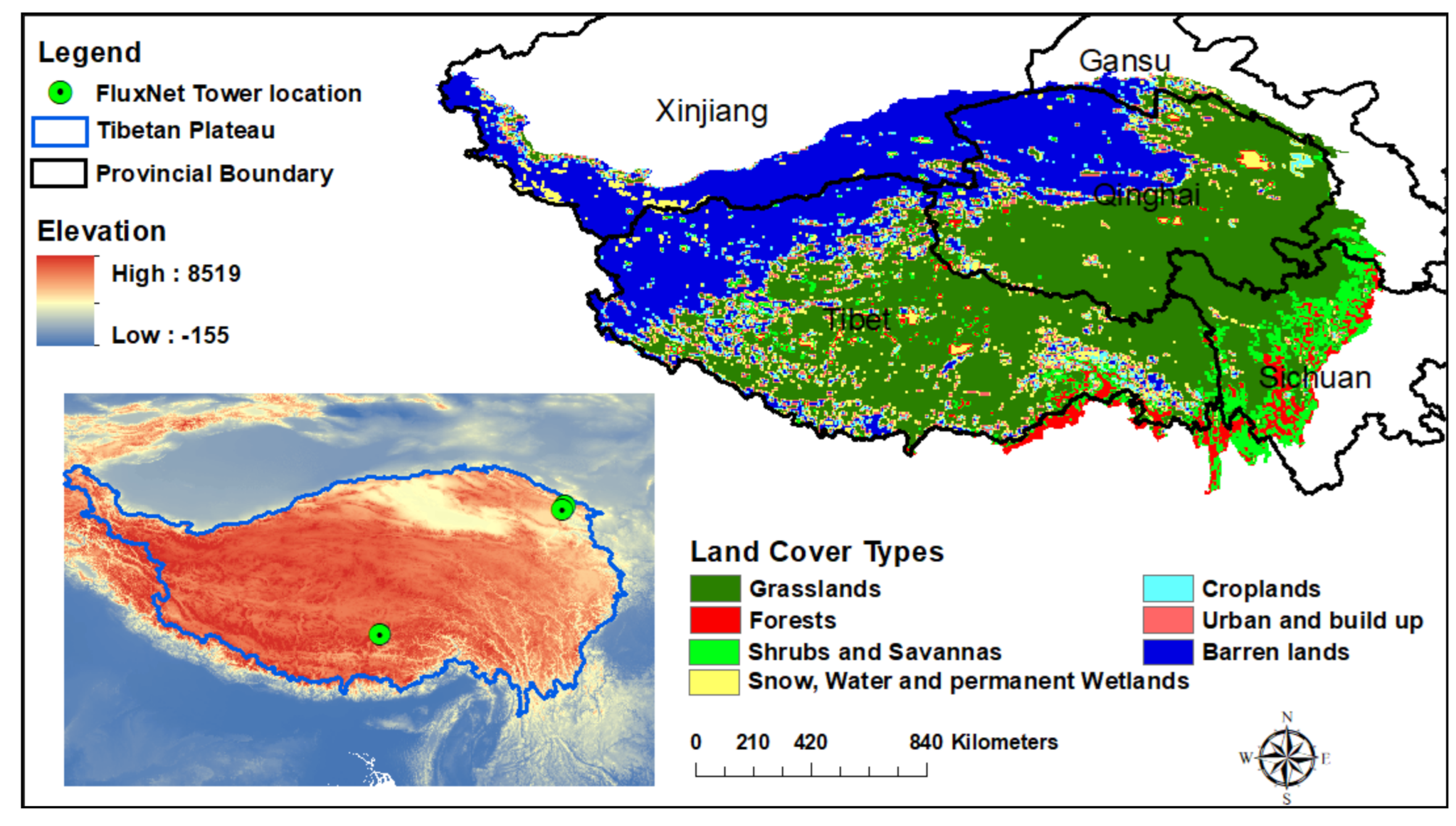
2. Study Area
3. Data and Methods
3.1. CERES Radiation Product
3.2. MODIS Products
3.3. Reanalysis Data
3.4. FluxNet Data
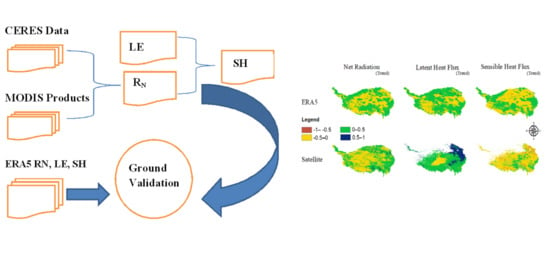
3.5. Derivation of SEB from Satellite Data
3.6. Comparison Ofmultiple Data Sources
3.7. Statistical Analysis
4. Results
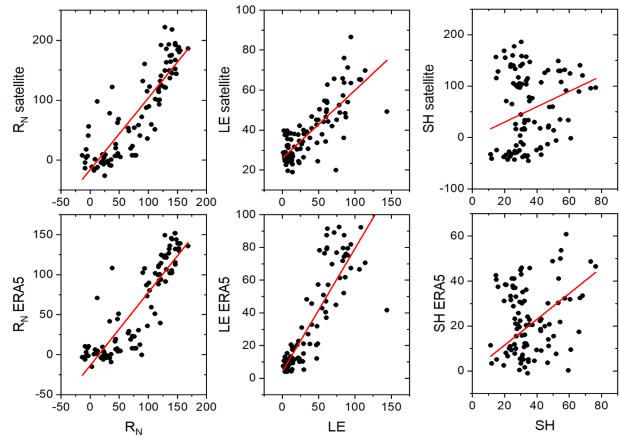
4.1. Validation of SEB Parameters
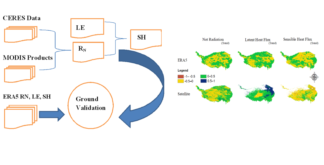
4.2. Spatio-Temporal Analysis
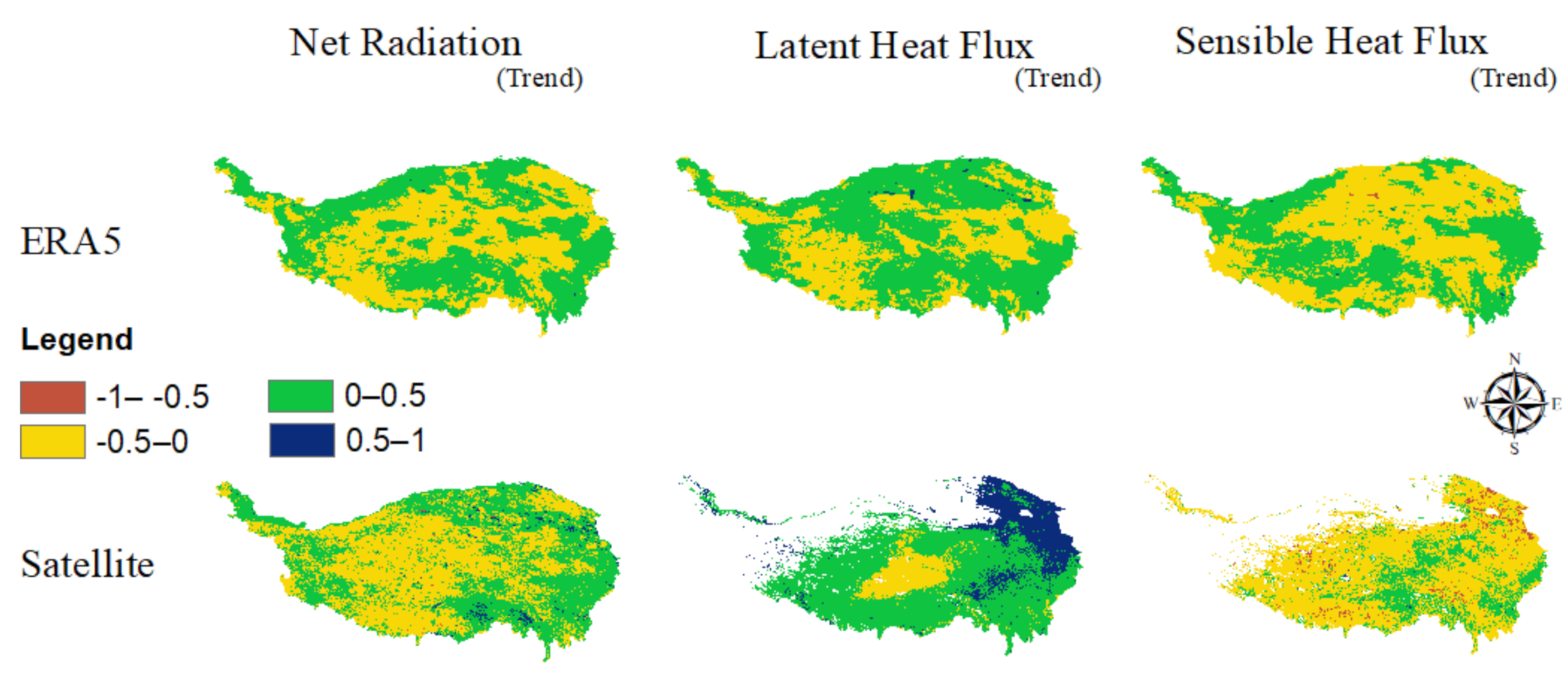
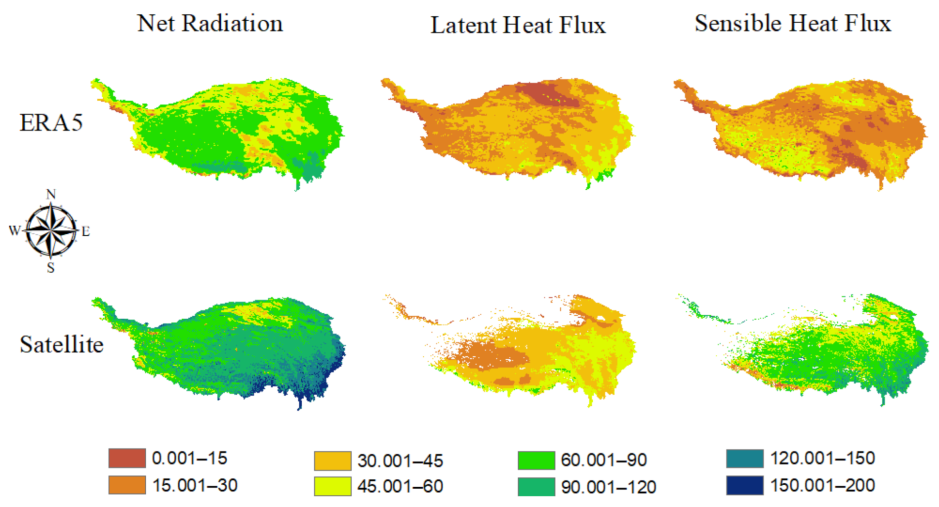
4.3. Spatial Analysis
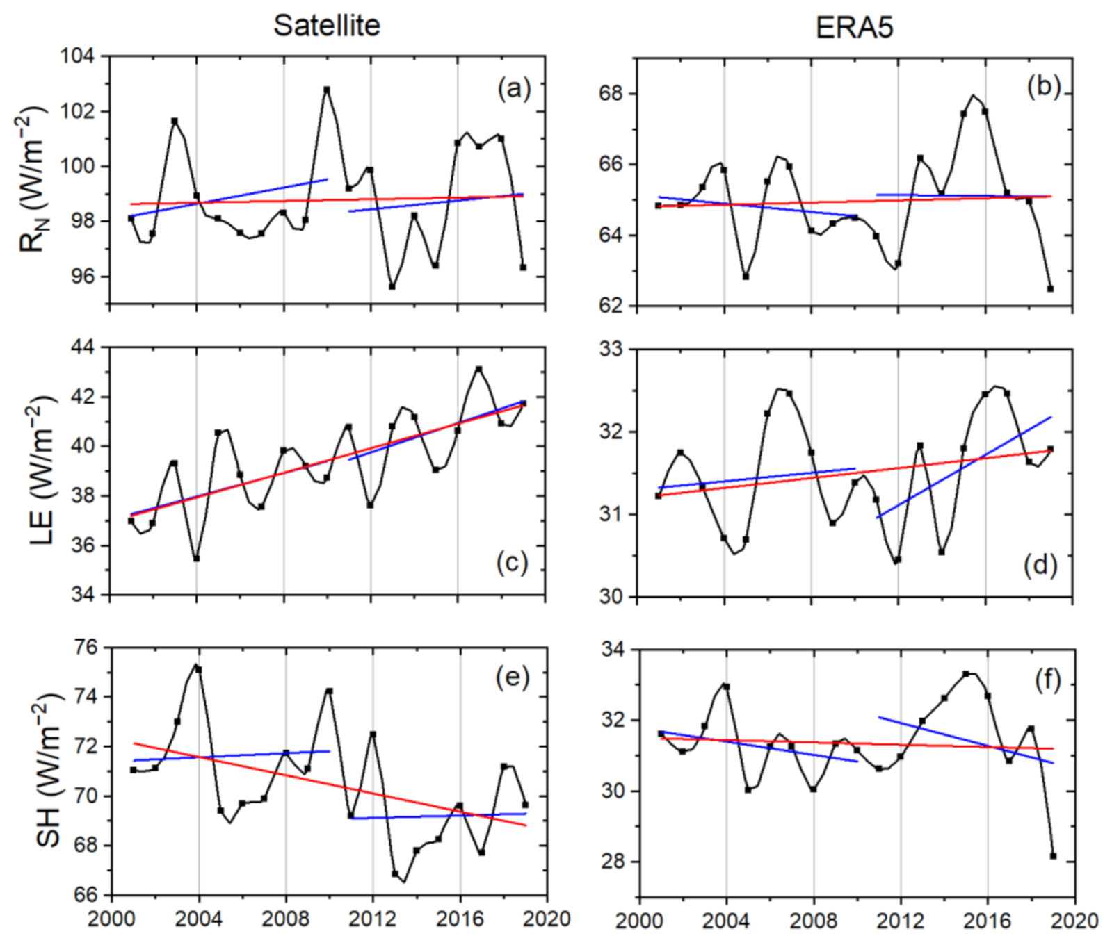
4.4. Temporal Analysis
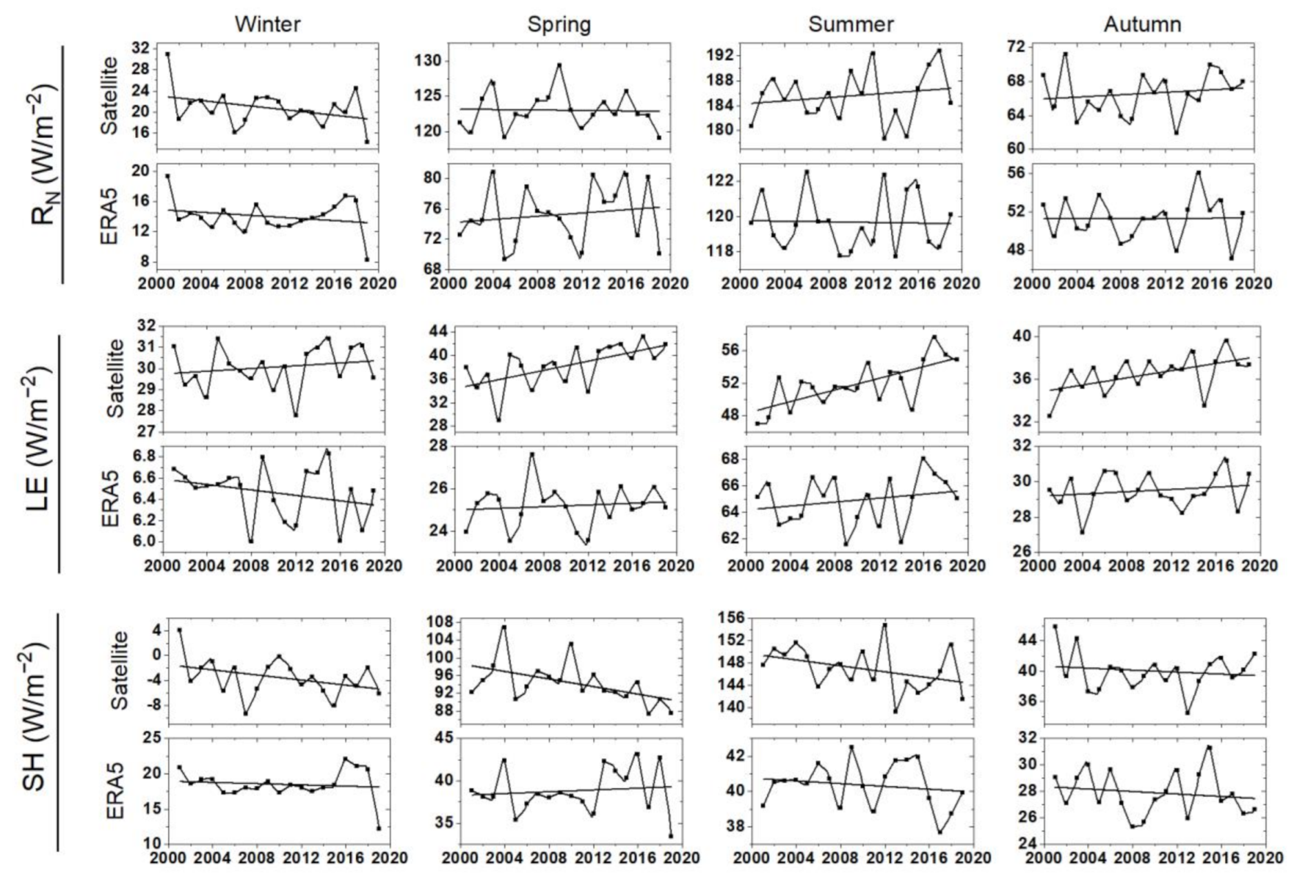
4.5. Seasonal Aanalysis
4.6. NDVI and LE
4.7. LST, Air Temperature and SH
5. Discussions
6. Conclusions
- (1)
- After validation from in situ ground observations, RN observed from satellite and ERA5 data are equally reliable and can be used for SEB studies. ERA5 LE is more accurate for monthly analysis, but for annual analysis satellite, LE product (MODIS MOD16A2) can be used as its MAE over a longer duration is less than the MAE of ERA5 LE. Although satellite SH is an efficient alternative over large spatial and longer temporal durations, in the current study it is less accurate than ERA5 SH, which showed better validation statistics in TP. Satellite and ERA5 data observations are in better agreement over forests, savannas and shrub lands, but for barren lands, both observations differ widely.
- (2)
- East and southeast regions of TP exhibit the prominent increasing trend for all SEB parameters, while central regions show decreasing trends. Temporally, a significant increase in LE is observed over TP while a relatively smaller decrease for SH is observed over the same period. RN shows the nominal increasing temporal trend.
- (3)
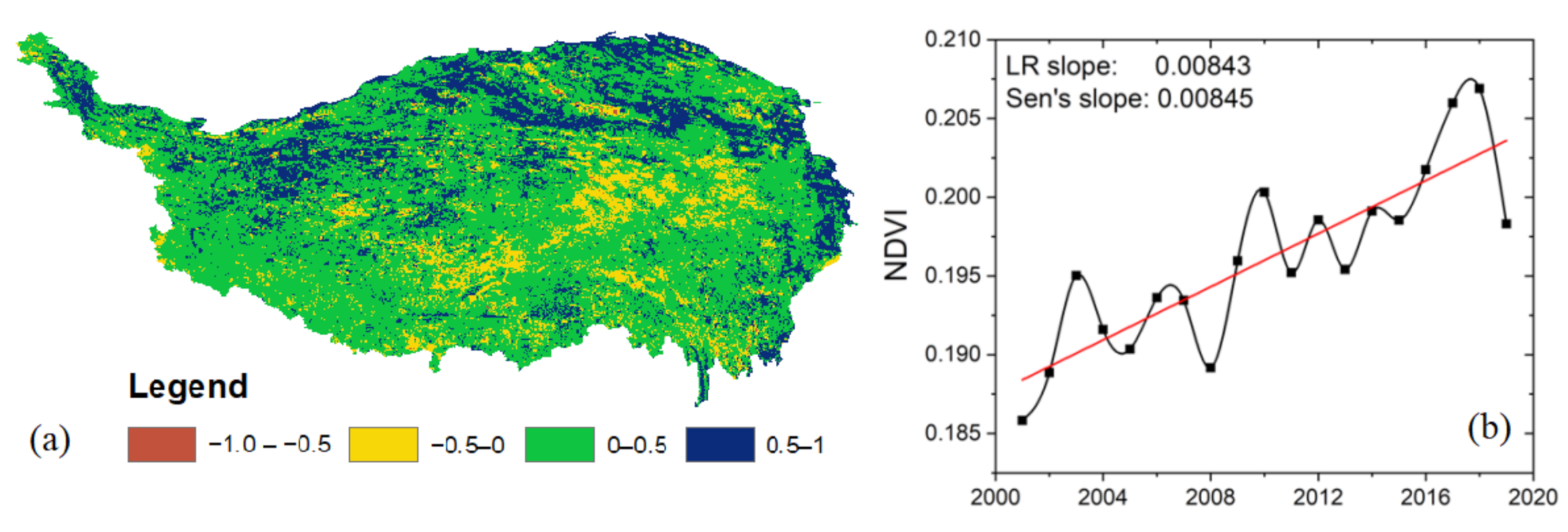
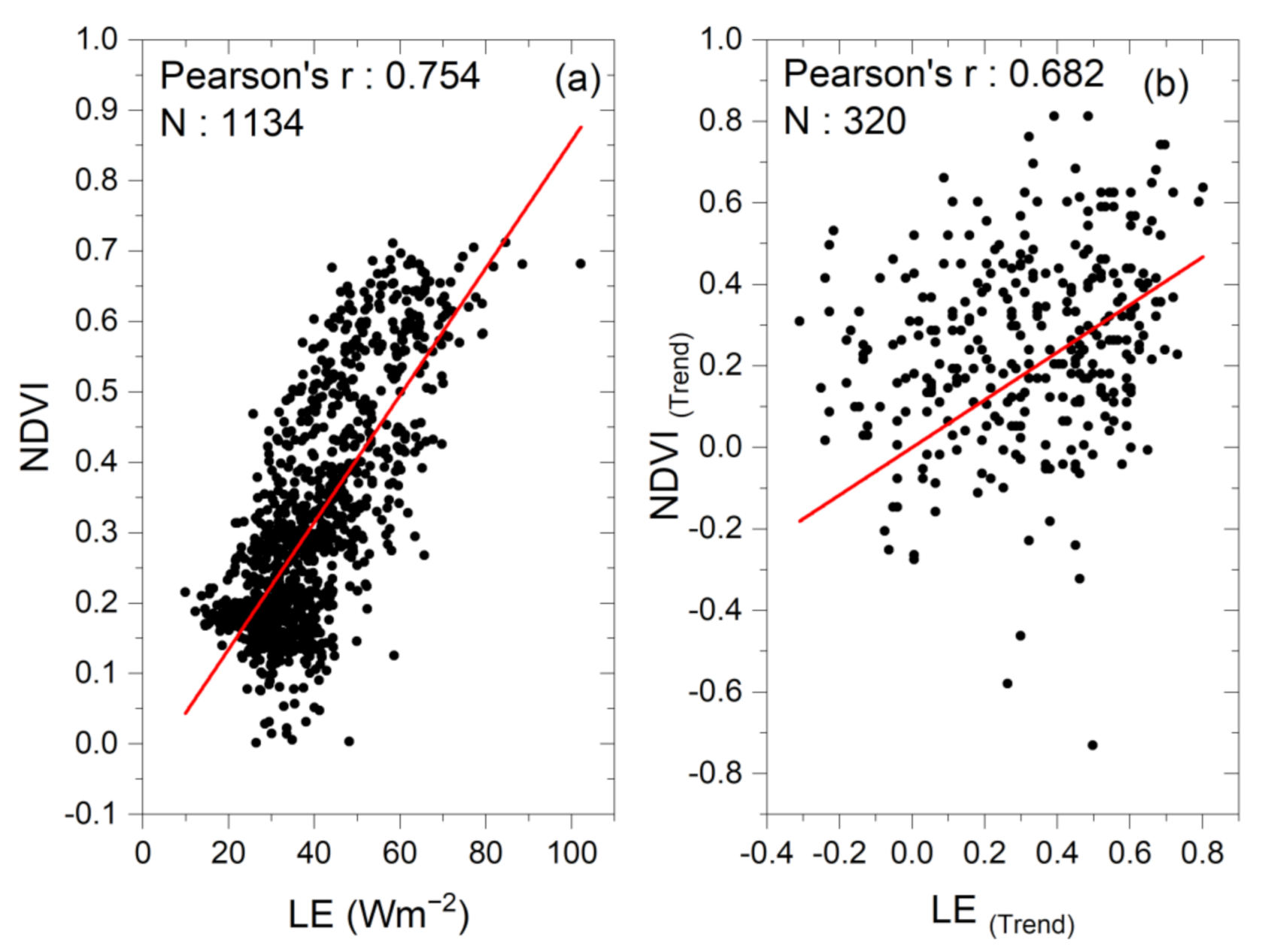
- NDVI is an important parameter not only for the land cover but also to analyze LE. Over TP, NDVI’s spatial, temporal, and spatio-temporal trends endorsed the trends of LE. Increasing NDVI also enlightens the growing vegetation cover over TP.
- (4)
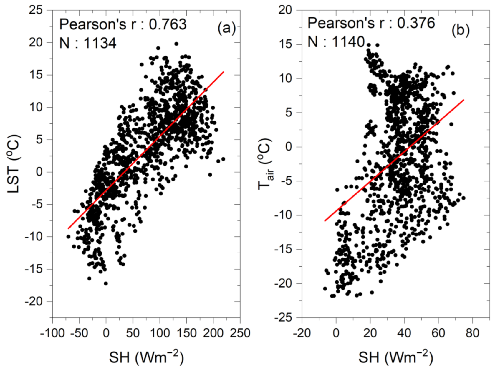
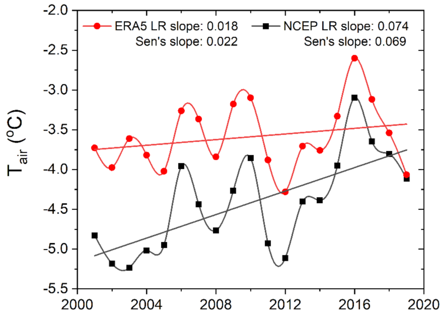
- SH is an important parameter for the heat cycle, yet it may not solely define the atmospheric temperature trends as SH is decreasing over TP but the air temperature is increasing in the region.
- (5)
- Climate warming and an imbalance between SEB parameters lead towards the thawing of permafrost and snow melting in TP. Being the water head of many important rivers of east and south Asia, any change in the heat cycle of TP enormously affects the whole region. As discussed earlier, TP has a major impact on the Asian monsoon; thus, an increase in LE may alter the Asian monsoon pattern and eventually the whole regional climate.
Author Contributions
Funding
Data Availability Statement
Acknowledgments
Conflicts of Interest
References
- Qiu, J. China: The third pole. Nature 2008, 454, 393–396. [Google Scholar] [CrossRef] [PubMed]
- Duan, A.; Li, F.; Wang, M.; Wu, G. Persistent weakening trend in the spring sensible heat source over the Tibetan Plateau and its impact on the Asian summer monsoon. J. Clim. 2011, 24, 5671–5682. [Google Scholar] [CrossRef]
- Shi, Q.; Liang, S. Surface-sensible and latent heat fluxes over the Tibetan Plateau from ground measurements, reanalysis, and satellite data. Atmos. Chem. Phys. 2014, 14, 5659–5677. [Google Scholar] [CrossRef]
- Duan, J.; Esper, J.; Büntgen, U.; Li, L.; Xoplaki, E.; Zhang, H.; Wang, L.; Fang, Y.; Luterbacher, J. Weakening of annual temperature cycle over the Tibetan Plateau since the 1870s. Nat. Commun. 2017, 8, 1–7. [Google Scholar] [CrossRef] [PubMed]
- Duan, J.; Li, L.; Fang, Y. Seasonal spatial heterogeneity of warming rates on the Tibetan Plateau over the past 30 years. Sci. Rep. 2015, 5, 1–8. [Google Scholar] [CrossRef]
- Xie, J.; Yu, Y.; Li, J.l.; Ge, J.; Liu, C. Comparison of surface sensible and latent heat fluxes over the Tibetan Plateau from reanalysis and observations. Meteorol. Atmos. Phys. 2019, 131, 567–584. [Google Scholar] [CrossRef]
- Immerzeel, W.W.; van Beek, L.P.H.; Bierkens, M.F.P. Climate change will affect the asian water towers. Science 2010, 328, 1382–1385. [Google Scholar] [CrossRef]
- Yao, T.; Xue, Y.; Chen, D.; Chen, F.; Thompson, L.; Cui, P.; Koike, T.; Lau, W.K.; Lettenmaier, D.; Mosbrugger, V.; et al. Recent third pole’s rapid warming accompanies cryospheric melt and water cycle intensification and interactions between monsoon and environment: Multidisciplinary approach with observations, modeling, and analysis. Bull. Am. Meteorol. Soc. 2019, 100, 423–444. [Google Scholar] [CrossRef]
- Wang, X.; Zheng, D.; Shen, Y. Land use change and its driving forces on the Tibetan Plateau during 1990–2000. Catena 2008, 72, 56–66. [Google Scholar] [CrossRef]
- Stephens, G.L.; Li, J.; Wild, M.; Clayson, C.A.; Loeb, N.; Kato, S.; L’ecuyer, T.; Stackhouse, P.W.; Lebsock, M.; Andrews, T. An update on Earth’s energy balance in light of the latest global observations. Nat. Geosci. 2012, 5, 691–696. [Google Scholar] [CrossRef]
- Anderson, R.G.; Canadell, J.G.; Randerson, J.T.; Jackson, R.B.; Hungate, B.A.; Baldocchi, D.D.; Ban-Weiss, G.A.; Bonan, G.B.; Caldeira, K.; Cao, L.; et al. Biophysical considerations in forestry for climate protection. Front. Ecol. Environ. 2011, 9, 174–182. [Google Scholar] [CrossRef]
- Wild, M.; Gilgen, H.; Roesch, A.; Ohmura, A.; Long, C.N.; Dutton, E.G.; Forgan, B.; Kallis, A.; Russak, V.; Tsvetkov, A. From dimming to brightening: Decadal changes in solar radiation at earth’s surface. Science 2005, 308, 847–850. [Google Scholar] [CrossRef] [PubMed]
- Nair, U.S.; Ray, D.K.; Wang, J.; Christopher, S.A.; Lyons, T.J.; Welch, R.M.; Pielke, R.A., Sr. Observational estimates of radiative forcing due to land use change in southwest Australia. J. Geophys. Res. Atmos. 2007, 112, 1–8. [Google Scholar] [CrossRef]
- Bright, R.M.; Davin, E.; O’Halloran, T.; Pongratz, J.; Zhao, K.; Cescatti, A. Local temperature response to land cover and management change driven by non-radiative processes. Nat. Clim. Chang. 2017, 7, 296–302. [Google Scholar] [CrossRef]
- He, T.; Shao, Q.; Cao, W.; Huang, L.; Liu, L. Satellite-observed energy budget change of deforestation in northeastern china and its climate implications. Remote Sens. 2015, 7, 11586–11601. [Google Scholar] [CrossRef]
- Bilal, M.; Nichol, J.E.; Nazeer, M. Validation of Aqua-MODIS C051 and C006 Operational Aerosol Products Using AERONET Measurements over Pakistan. IEEE J. Sel. Top. Appl. Earth Obs. Remote Sens. 2016, 9, 2074–2080. [Google Scholar] [CrossRef]
- Ali, M.A.; Islam, M.M.; Islam, M.N.; Almazroui, M. Investigations of MODIS AOD and cloud properties with CERES sensor based net cloud radiative effect and a NOAA HYSPLIT Model over Bangladesh for the period 2001–2016. Atmos. Res. 2019, 215, 268–283. [Google Scholar] [CrossRef]
- Davin, E.L.; de Noblet-Ducoudre, N. Climatic impact of global-scale Deforestation: Radiative versus nonradiative processes. J. Clim. 2010, 23, 97–112. [Google Scholar] [CrossRef]
- Houspanossian, J.; Nosetto, M.; Jobbágy, E.G. Radiation budget changes with dry forest clearing in temperate Argentina. Glob. Chang. Biol. 2013, 19, 1211–1222. [Google Scholar] [CrossRef]
- Shen, M.; Piao, S.; Jeong, S.J.; Zhou, L.; Zeng, Z.; Ciais, P.; Chen, D.; Huang, M.; Jin, C.S.; Li, L.Z.; et al. Evaporative cooling over the Tibetan Plateau induced by vegetation growth. Proc. Natl. Acad. Sci. USA 2015, 112, 9299–9304. [Google Scholar] [CrossRef]
- Myhre, G.; Samset, B.H.; Hodnebrog, Ø.; Andrews, T.; Boucher, O.; Faluvegi, G.; Fläschner, D.; Forster, P.M.; Kasoar, M.; Kharin, V.; et al. Sensible heat has significantly affected the global hydrological cycle over the historical period. Nat. Commun. 2018, 9, 1–9. [Google Scholar] [CrossRef] [PubMed]
- Ma, Y.; Su, Z.; Koike, T.; Yao, T.; Ishikawa, H.; Ueno, K.I.; Menenti, M. On measuring and remote sensing surface energy partitioning over the Tibetan Plateau-from GAME/Tibet to CAMP/Tibet. Phys. Chem. Earth 2003, 28, 63–74. [Google Scholar] [CrossRef]
- Wang, Y.; Xu, X.; Liu, H.; Li, Y.; Li, Y.; Hu, Z.; Gao, X.; Ma, Y.; Sun, J.; Lenschow, D.H.; et al. Analysis of land surface parameters and turbulence characteristics over the Tibetan Plateau and surrounding region. J. Geophys. Res. 2016, 121, 9540–9560. [Google Scholar] [CrossRef]
- Zhao, P.; Xu, X.; Chen, F.; Guo, X.; Zheng, X.; Liu, L.; Hong, Y.; Li, Y.; La, Z.; Peng, H.; et al. The third atmospheric scientific experiment for understanding the earth–Atmosphere coupled system over the tibetan plateau and its effects. Bull. Am. Meteorol. Soc. 2018, 99, 757–776. [Google Scholar] [CrossRef]
- Xin, Y.F.; Chen, F.; Zhao, P.; Barlage, M.; Blanken, P.; Chen, Y.L.; Chen, B.; Wang, Y.J. Surface energy balance closure at ten sites over the Tibetan plateau. Agric. For. Meteorol. 2018, 259, 317–328. [Google Scholar] [CrossRef]
- Tanaka, K.; Ishikawa, H.; Hayashi, T.; Tamagawa, I.; Yaoming, M. Surface energy budget at Amdo on the Tibetan plateau using GAME/Tibet IOP98 data. J. Meteorol. Soc. Jpn 2001, 79, 505–517. [Google Scholar] [CrossRef]
- You, Q.; Min, J.; Kang, S. Rapid warming in the tibetan plateau from observations and CMIP5 models in recent decades. Int. J. Climatol. 2016, 36, 2660–2670. [Google Scholar] [CrossRef]
- Cai, D.; You, Q.; Fraedrich, K.; Guan, Y. Spatiotemporal temperature variability over the Tibetan Plateau: Altitudinal dependence associated with the global warming hiatus. J. Clim. 2017, 30, 969–984. [Google Scholar] [CrossRef]
- Yan, Y.; You, Q.; Wu, F.; Pepin, N.; Kang, S. Surface mean temperature from the observational stations and multiple reanalyses over the Tibetan Plateau. Clim. Dyn. 2020, 55, 2405–2419. [Google Scholar] [CrossRef]
- Duan, A.; Wang, M.; Lei, Y.; Cui, Y. Trends in summer rainfall over china associated with the Tibetan Plateau sensible heat source during 1980–2008. J. Clim. 2013, 26, 261–275. [Google Scholar] [CrossRef]
- Wang, K.; Ma, Q.; Li, Z.; Wang, J. Decadal variability of surface incident solar radiation over China: Observations, satellite retrievals, and reanalyses. J. Geophys. Res. Atmos. 2015, 120, 6500–6514. [Google Scholar] [CrossRef]
- Zhou, Z.; Wang, L.; Lin, A.; Zhang, M.; Niu, Z. Innovative trend analysis of solar radiation in China during 1962–2015. Renew. Energy 2018, 119, 675–689. [Google Scholar] [CrossRef]
- Yang, K.; Guo, X.F.; Wu, B.Y. Recent trends in surface sensible heat flux on the Tibetan Plateau. Sci. China Earth Sci. 2011, 54, 19–28. [Google Scholar] [CrossRef]
- Zhu, X.Y.; Liu, Y.M.; Wu, G.X. An assessment of summer sensible heat flux on the Tibetan Plateau from eight data sets. Sci. China Earth Sci. 2012, 55, 779–786. [Google Scholar] [CrossRef]
- Zhou, L.T.; Huang, R. Regional differences in surface sensible and latent heat fluxes in China. Theor. Appl. Climatol. 2014, 116, 625–637. [Google Scholar] [CrossRef]
- Liang, S.; Kustas, W.; Schaepman-Strub, G.; Li, X. Impacts of climate change and land use changes on land surface radiation and energy budgets. IEEE J. Sel. Top. Appl. Earth Obs. Remote Sens. 2010, 3, 219–224. [Google Scholar] [CrossRef]
- Liang, S.; Wang, D.; He, T.; Yu, Y. Remote sensing of earth’s energy budget: Synthesis and review. Int. J. Digit. Earth 2019, 12, 737–780. [Google Scholar] [CrossRef]
- Duveiller, G.; Hooker, J.; Cescatti, A. The mark of vegetation change on Earth’s surface energy balance. Nat. Commun. 2018, 9, 679. [Google Scholar] [CrossRef]
- Kandel, R.; Viollier, M. Observation of the Earth’s radiation budget from space. C. R. Geosci. 2010, 342, 286–300. [Google Scholar] [CrossRef]
- Cui, X.; Graf, H.F. Recent land cover changes on the Tibetan Plateau: A review. Clim. Change 2009, 94, 47–61. [Google Scholar] [CrossRef]
- Liu, X.; Chen, B. Climatic warming in the Tibetan Plateau during recent decades. Int. J. Climatol. 2000, 20, 1729–1742. [Google Scholar] [CrossRef]
- Liu, X.; Yin, Z.Y. Sensitivity of East Asian monsoon climate to the uplift of the Tibetan Plateau. Palaeogeogr. Palaeoclimatol. Palaeoecol. 2002, 183, 223–245. [Google Scholar] [CrossRef]
- Yili, Z.; Bingyu, L.; Du, Z. Datasets of the boundary and area of the Tibetan Plateau ZHANG. Acta Geogr. Sin. 2014, 69, 140–143. [Google Scholar]
- Loeb, N.G.; Doelling, D.R.; Wang, H.; Su, W.; Nguyen, C.; Corbett, J.G.; Liang, L.; Mitrescu, C.; Rose, F.G.; Kato, S. Clouds and the Earth’S Radiant Energy System (CERES) Energy Balanced and Filled (EBAF) top-of-atmosphere (TOA) edition-4.0 data product. J. Clim. 2018, 31, 895–918. [Google Scholar] [CrossRef]
- Su, W.; Corbett, J.; Eitzen, Z.; Liang, L. Next-generation angular distribution models for top-of-atmosphere radiative flux calculation from CERES instruments: Methodology. Atmos. Meas. Tech. 2015, 8, 611–632. [Google Scholar] [CrossRef]
- Fu, Q.; Liou, K.N. Parameterization of the radiative properties of cirrus clouds. J. Atmos. Sci. 1993, 50, 2008–2025. [Google Scholar] [CrossRef]
- Kato, S.; Rose, F.G.; Rutan, D.A.; Thorsen, T.J.; Loeb, N.G.; Doelling, D.R.; Huang, X.; Smith, W.L.; Su, W.; Ham, S.H. Surface irradiances of edition 4.0 Clouds and the Earth’s Radiant Energy System (CERES) Energy Balanced and Filled (EBAF) data product. J. Clim. 2018, 31, 4501–4527. [Google Scholar] [CrossRef]
- Schaaf, C.B.; Gao, F.; Strahler, A.H.; Lucht, W.; Li, X.; Tsang, T.; Strugnell, N.C.; Zhang, X.; Jin, Y.; Muller, J.P.; et al. First operational BRDF, albedo nadir reflectance products from MODIS. Remote Sens. Environ. 2002, 83, 135–148. [Google Scholar] [CrossRef]
- Schaaf, C.B.; Liu, J.; Gao, F.; Strahler, A.H. Aqua and terra MODIS albedo and reflectance anisotropy products. In Remote Sensing and Digital Image Processing; Springer: New York, NY, USA,, 2011; Volume 11, pp. 549–561. [Google Scholar]
- Li, Y.; Zhao, M.; Motesharrei, S.; Mu, Q.; Kalnay, E.; Li, S. Local cooling and warming effects of forests based on satellite observations. Nat. Commun. 2015, 6, 1–8. [Google Scholar] [CrossRef]
- Wan, Z. A generalized split-window algorithm for retrieving land-surface temperature from space. IEEE Trans. Geosci. Remote Sens. 1996, 34, 892–905. [Google Scholar]
- Snyder, W.C.; Wan, Z. BRDF models to predict spectral reflectance and emissivity in the thermal infrared. IEEE Trans. Geosci. Remote Sens. 1998, 36, 214–225. [Google Scholar] [CrossRef]
- Bilal, M.; Nichol, J.E.; Wang, L. New customized methods for improvement of the MODIS C6 Dark Target and Deep Blue merged aerosol product. Remote Sens. Environ. 2017, 197, 115–124. [Google Scholar] [CrossRef]
- Bilal, M.; Qiu, Z.; Campbell, J.R.; Spak, S.N.; Shen, X.; Nazeer, M. A new MODIS C6 dark target and Deep Blue merged aerosol product on a 3 km spatial grid. Remote Sens. 2018, 10, 463. [Google Scholar] [CrossRef]
- Wan, Z. New refinements and validation of the collection-6 MODIS land-surface temperature/emissivity product. Remote Sens. Environ. 2014, 140, 36–45. [Google Scholar] [CrossRef]
- Wang, K.; Wan, Z.; Wang, P.; Sparrow, M.; Liu, J.; Haginoya, S. Evaluation and improvement of the MODIS land surface temperature/emissivity products using ground-based measurements at a semi-desert site on the western Tibetan Plateau. Int. J. Remote Sens. 2007, 28, 2549–2565. [Google Scholar] [CrossRef]
- Mu, Q.; Zhao, M.; Running, S.W. Improvements to a MODIS global terrestrial evapotranspiration algorithm. Remote Sens. Environ. 2011, 115, 1781–1800. [Google Scholar] [CrossRef]
- Mu, Q.; Heinsch, F.A.; Zhao, M.; Running, S.W. Development of a global evapotranspiration algorithm based on MODIS and global meteorology data. Remote Sens. Environ. 2007, 111, 519–536. [Google Scholar] [CrossRef]
- Huete, A.; Didan, K.; Miura, T.; Rodriguez, E.P.; Gao, X.; Ferreira, L.G. Overview of the radiometric and biophysical performance of the MODIS vegetation indices. Remote Sens. Environ. 2002, 83, 195–213. [Google Scholar] [CrossRef]
- Vermote, E.F.; el Saleous, N.Z.; Justice, C.O. Atmospheric correction of MODIS data in the visible to middle infrared: First results. Remote Sens. Environ. 2002, 83, 97–111. [Google Scholar] [CrossRef]
- Hersbach, H.; Bell, B.; Berrisford, P.; Hirahara, S.; Horányi, A.; Muñoz-Sabater, J.; Nicolas, J.; Peubey, C.; Radu, R.; Schepers, D.; et al. The ERA5 global reanalysis. Q. J. R. Meteorol. Soc. 2020, 146, 1999–2049. [Google Scholar] [CrossRef]
- Park, S. IFS Doc-Physical Processes; IFS Documentation CY45R1, no. 1. ECMWF, 2018; pp. 1–223. Available online: https://www.ecmwf.int/en/elibrary/18714-part-iv-physical-processes (accessed on 11 January 2021).
- Kalnay, E.; Kanamitsu, M.; Kistler, R.; Collins, W.; Deaven, D.; Gandin, L.; Iredell, M.; Saha, S.; White, G.; Woollen, J.; et al. The NCEP/NCAR 40-year reanalysis project. Bull. Am. Meteorol. Soc. 1996, 77, 437–471. [Google Scholar] [CrossRef]
- Shi, P.; Sun, X.; Xu, L.; Zhang, X.; He, Y.; Zhang, D.; Yu, G. Net ecosystem CO2 exchange and controlling factors in a steppe-Kobresia meadow on the Tibetan Plateau. Sci. China Ser. D Earth Sci. 2006, 49, 207–218. [Google Scholar] [CrossRef]
- Kato, T.; Tang, Y.; Gu, S.; Hirota, M.; Du, M.; Li, Y.; Zhao, X. Temperature and biomass influences on interannual changes in CO2 exchange in an alpine meadow on the Qinghai-Tibetan Plateau. Glob. Chang. Biol. 2006, 12, 1285–1298. [Google Scholar] [CrossRef]
- Bastiaanssen, W.G.M.; Cheema, M.J.M.; Immerzeel, W.W.; Miltenburg, I.J.; Pelgrum, H. Surface energy balance and actual evapotranspiration of the transboundary Indus Basin estimated from satellite measurements and the ETLook model. Water Resour. Res. 2012, 48, 1–16. [Google Scholar] [CrossRef]
- Kendall, M.G. Rank Correlation Methods; Griffin: Oxford, UK, 1948. [Google Scholar]
- Mann, H.B. Nonparametric Tests Against Trend. Econometrica 1945, 13, 245–259. [Google Scholar] [CrossRef]
- Ma, W.; Jia, G.; Zhang, A. Multiple satellite-based analysis reveals complex climate effects of temperate forests and related energy budget. J. Geophys. Res. 2017, 122, 3806–3820. [Google Scholar] [CrossRef]
- Miehe, G.; Miehe, S.; Koch, K.; Will, M. Sacred Forests in Tibet. Mt. Res. Dev. 2003, 23, 324–328. [Google Scholar] [CrossRef]


| Site ID | Site Name | Latitude | Longitude | Land cover | Duration |
|---|---|---|---|---|---|
| CN-Dan | Dangxiong | 30.4978° | 91.066° | Grassland | 2004–05 |
| CN-Ha2 | Haibei Shrubland | 37.6086° | 101.3269° | Wetland | 2003–05 |
| CN-HaM | Haibei Alpine Tibet Site | 37.3700° | 101.1800° | Grassland | 2002–04 |
| Sensor/Source | Product | Parameter | Spatial Resolution | Temporal Resolution |
|---|---|---|---|---|
| MODIS | MCD43C3 | Albedo | 0.05° | Daily |
| MODIS | MOD11C3 | LST | 0.05° | Monthly |
| MODIS | MOD11C3 | Emissivity | 0.05° | Monthly |
| MODIS | MOD16A2 | LE | 500 m | 8-days |
| MODIS | MOD13C2 | NDVI | 0.05° | Monthly |
| MODIS | MCD12C1 | Land Cover | 0.05° | Annual |
| CERES | EBAF-surface | Incoming SW | 1° | Monthly |
| CERES | EBAF-surface | Incoming LW | 1° | Monthly |
| ERA5 | Land monthly averaged | Net SW | 0.1° | Monthly |
| ERA5 | Land monthly averaged | Net LW | 0.1° | Monthly |
| ERA5 | Land monthly averaged | LE | 0.1° | Monthly |
| ERA5 | Land monthly averaged | SH | 0.1° | Monthly |
| ERA5 | Land monthly averaged | Temperature | 0.1° | Monthly |
| NCEP | Air temperature at 2m | Temperature | 2.5° | Monthly |
| FluxNET | FluxNET-2015 | RN, LE,SH | Point data | Monthly |
| Statistical Analysis | RN (Wm−2) | LE (Wm−2) | SH (Wm−2) | |||
|---|---|---|---|---|---|---|
| ERA5 | Satellite | ERA5 | Satellite | ERA5 | Satellite | |
| LR Slope | 0.91 ** | 1.19 ** | 0.75 ** | 0.35 ** | 0.75 * | 1.49 |
| Pearson’s r | 0.88 ** | 0.87 ** | 0.86 ** | 0.79 ** | 0.81 * | 0.63 |
| MBE (Wm−2) | 20.53 | 0.33 | 5.55 | −0.37 | 13.19 | −21.8 |
| MAE (Wm−2) | 26.39 | 30.03 | 11.59 | 18.98 | 18.93 | 62.85 |
| Duration | ERA5 | Satellite | |||
|---|---|---|---|---|---|
| LR Slope | Sen’s Slope | LR Slope | Sen’s Slope | ||
| RN | 2001–10 | −0.06 ± 0.1 | −0.04 | 0.15 ± 0.2 | 0.007 |
| 2011–19 | −0.005 ± 0.2 | −0.03 | 0.08 ± 0.2 | 0.18 | |
| 2001–19 | 0.01 ± 0.05 | 0.02 | 0.01 ± 0.08 | 0.03 | |
| LE | 2001–10 | 0.02 ± 0.7 | 0.02 | 0.24 ± 0.1 | 0.19 |
| 2011–19 | 0.15 ± 0.08 | 0.15 | 0.29 ± 0.1 | 0.25 ** | |
| 2001–19 | 0.03 ± 0.02 | 0.03 | 0.25 ± 0.05 ** | 0.25 ** | |
| SH | 2001–10 | −0.09 ± 0.9 | −0.05 | 0.04 ± 0.2 | 0.11 |
| 2011–19 | −0.16 ± 0.2 | 0.006 | 0.02 ± 0.2 | 0.15 | |
| 2001–19 | −0.02 ± 0.05 | 0.005 | −0.18 ± 0.08 * | −0.18 * | |
| Data Set | Winter | Spring | Summer | Autumn | |
|---|---|---|---|---|---|
| RN | Satellite | −0.23 ± 0.1 * | −0.02 ± 0.1 | 0.13 ± 0.1 | 0.07 ± 0.1 |
| ERA5 | −0.09 ± 0.09 | 0.11 ± 0.1 | −0.008 ± 0.06 | 0.003 ± 0.09 | |
| LE | Satellite | 0.03 ± 0.04 | 0.39 ± 0.1 ** | 0.36 ± 0.08 ** | 0.17 ± 0.06 * |
| ERA5 | −0.01 ± 0.01 | 0.02 ± 0.04 | 0.07 ± 0.07 | 0.03 ± 0.04 | |
| SH | Satellite | −0.2 ± 0.1 * | −0.43 ± 0.1 ** | −0.27 ± 0.1 * | −0.06 ± 0.1 |
| ERA5 | −0.04 ± 0.08 | 0.05 ± 0.1 | −0.04 ± 0.05 | −0.05 ± 0.06 | |
| Statistical Analysis | RN | LE | SH |
|---|---|---|---|
| MBE (Wm−2) | 34.02 | 7.55 | 38.27 |
| MAE (Wm−2) | 34.39 | 15.58 | 53.92 |
Publisher’s Note: MDPI stays neutral with regard to jurisdictional claims in published maps and institutional affiliations. |
© 2021 by the authors. Licensee MDPI, Basel, Switzerland. This article is an open access article distributed under the terms and conditions of the Creative Commons Attribution (CC BY) license (http://creativecommons.org/licenses/by/4.0/).
Share and Cite
Mazhar, U.; Jin, S.; Duan, W.; Bilal, M.; Ali, M.A.; Farooq, H. Spatio-Temporal Trends of Surface Energy Budget in Tibet from Satellite Remote Sensing Observations and Reanalysis Data. Remote Sens. 2021, 13, 256. https://doi.org/10.3390/rs13020256
Mazhar U, Jin S, Duan W, Bilal M, Ali MA, Farooq H. Spatio-Temporal Trends of Surface Energy Budget in Tibet from Satellite Remote Sensing Observations and Reanalysis Data. Remote Sensing. 2021; 13(2):256. https://doi.org/10.3390/rs13020256
Chicago/Turabian StyleMazhar, Usman, Shuanggen Jin, Wentao Duan, Muhammad Bilal, Md. Arfan Ali, and Hasnain Farooq. 2021. "Spatio-Temporal Trends of Surface Energy Budget in Tibet from Satellite Remote Sensing Observations and Reanalysis Data" Remote Sensing 13, no. 2: 256. https://doi.org/10.3390/rs13020256
APA StyleMazhar, U., Jin, S., Duan, W., Bilal, M., Ali, M. A., & Farooq, H. (2021). Spatio-Temporal Trends of Surface Energy Budget in Tibet from Satellite Remote Sensing Observations and Reanalysis Data. Remote Sensing, 13(2), 256. https://doi.org/10.3390/rs13020256