Abstract
Being the highest and largest land mass of the earth, the Tibetan Plateau has a strong impact on the Asian climate especially on the Asian monsoon. With high downward solar radiation, the Tibetan Plateau is a climate sensitive region and the main water source for many rivers in South and East Asia. Although many studies have analyzed energy fluxes in the Tibetan Plateau, a long-term detailed spatio-temporal variability of all energy budget parameters is not clear for understanding the dynamics of the regional climate change. In this paper, satellite remote sensing and reanalysis data are used to quantify spatio-temporal trends of energy budget parameters, net radiation, latent heat flux, and sensible heat flux over the Tibetan Plateau from 2001 to 2019. The validity of both data sources is analyzed from in situ ground measurements of the FluxNet micrometeorological tower network, which verifies that both datasets are valid and reliable. It is found that the trend of net radiation shows a slight increase. The latent heat flux increases continuously, while the sensible heat flux decreases continuously throughout the study period over the Tibetan Plateau. Varying energy fluxes in the Tibetan plateau will affect the regional hydrological cycle. Satellite LE product observation is limited to certain land covers. Thus, for larger spatial areas, reanalysis data is a more appropriate choice. Normalized difference vegetation index proves a useful indicator to explain the latent heat flux trend. Despite the reduction of sensible heat, the atmospheric temperature increases continuously resulting in the warming of the Tibetan Plateau. The opposite trend of sensible heat flux and air temperature is an interesting and explainable phenomenon. It is also concluded that the surface evaporative cooling is not the indicator of atmospheric cooling/warming. In the future, more work shall be done to explain the mechanism which involves the complete heat cycle in the Tibetan Plateau.
1. Introduction
The Tibetan Plateau (TP) is one of the largest reservoirs of ice and is referred to as the third pole of the world [1]. Due to its vast area and exceptional height (>4000 m above mean sea level), it plays a major role in shaping the regional climate especially for the east and south Asian monsoon [2,3]. TP is a climate-sensitive region with different climate change behavior from the surrounding regions [4,5]. According to some studies, the warming rate of TP is 0.3 °C per decade, which is more than any other part of the world. This affects permafrost and snow melting in TP. Eventually, freshwater reservoirs deplete at an alarming rate. Moreover, any change in the uplifted land affects the Asian monsoon upon which millions of people and thousands of hectares of crops depend [1,2,4,6,7,8].
Incoming solar radiation flux is high over TP [9], which has an important impact on the energy budget. The surface energy budget (SEB) derives the local climate and shapes the heat and water cycle [10]. SEB comprises mainly three parameters; (i) net radiation (RN), (ii) latent heat flux (LE), and (iii) sensible heat flux (SH). RN, as suggested by its name, is the radiative energy comprised of incoming and outgoing solar and thermal radiations. Land cover changes such as deforestation or snow melting influence RN because of the changing behavior of surface reflectivity in the form of albedo and land surface temperature (LST) [11,12,13,14,15]. The aerosol optical depth and atmospheric greenhouse gasses also influenced the RN through the atmospheric counter radiation [16,17]. LE is the non-radiative energy flux, and transfer energy in the form of change of state of matter (vaporization) [18]. Since vegetation cover involves largely in evapotranspiration, the vegetation index such as Normalized Difference Vegetation Index (NDVI) is a useful tool to analyze LE and its variability [19,20]. SH contributes to the non-radiative part of the SEB along with LE and relates to the heat cycle [2,21]. Transfer of heat between the surface and aloft air depends upon their temperature difference. SH is an important indicator but may not be the only triggering force for atmospheric temperature as wind speed, wind direction, and relative humidity also have a strong impact on air temperature.
There are plenty of great achievements that have been made in understanding climate change over TP. Many dedicated research programs have been launched to study TP climate such as the first, second, and third Tibetan Plateau Meteorological Science Experiment (TIPEX); the Global Energy and Water Cycle Experiment (GEWEX) of the Asian Monsoon Experiment in Tibet (GAME/Tibet); and the Coordinated and Enhanced Observation Period (CEOP) of the Asian-Australian Monsoon Project in Tibet (CAMP/Tibet). These projects provide quality of ground-based measurements [22,23,24,25,26]. Many recent studies observed atmospheric and surface warming in TP during the past few decades. Many researchers used ground station data and reanalysis data while few studies used satellite data to observe surface temperature [8,27,28,29]. Duan et al. [5] discussed heterogeneity of TP warming rates, pointing out that the northern TP had a higher warming rate than the southern TP, suggesting the higher precipitation of the southern TP as a potential cause of this heterogenetic behavior. Duan et al. [4] observed the weakening of the annual temperature cycle and associated this weakening with anthropogenic activities since the late nineteenth century. The snow melting and precipitation have a strong impact on regional climate eventually affecting the local population and crop production [7,30]. Few recent studies analyzed different trend analysis methods such as Mann–Kendall trend, linear regression and innovative trend analysis while others used different data sets to analyze annual and seasonal trends of downward solar radiation over TP [31,32].
Shen et al. [20] observed evaporative cooling using multiple data sources including satellite remote sensing and meteorological station data and established a strong link between NDVI and evaporative cooling in TP. SH trends especially in summer seasons were widely studied using reanalysis data sets and ground-based measurements. A decreasing trend for SH over TP was observed from many recent studies [2,33,34]. Many interesting recent studies observed SH and LE over TP using reanalysis data and ground measurements [3,35]. Xie et al. [6] observed the different trends for SH and LE from three different reanalysis data sets including ERA-Interim, JRA-55, and MERRA. Xin et al. [25] studied SEB ratio over TP from 10 ground-based measurements for July–October 2014 and analyzed the impact of atmospheric stability, friction velocity, turbulent temperature scale, and wind direction on SEB ratio.
Although TP has been widely studied for the SEB, there is still a gap for the detailed study of the trends of all major SEB parameters over a broader spatial and temporal coverage. Many factors such as land cover change, anthropogenic activities, altitude, latitudinal association, and local climatic conditions influence the spatio-temporal pattern of SEB [36,37,38]. This multidimensional phenomenon demands vast spatial and temporal coverage. Satellite remote sensing is an important tool to study long term SEB trends [39]. An alternative appropriate choice is the global climatic reanalysis data sets which are available for a longer historical duration on the global scale. In the current study, the trends of SEB over TP from satellite remote sensing data are analyzed and compared with reanalysis data for the period of 2001 to 2019. Moderate Resolution Imaging Spectroradiometer (MODIS) and Clouds and Earth’s Radiant Energy System (CERES) are used as satellite data sources, while ERA5 product released by European Centre for Medium-range Weather Forecasts (ECMWF) is used as the reanalysis data source. The main objectives of this study are to study (i) how the SEB varied in TP over the past two decades and (ii) the difference in SEB trends between satellite observations and reanalysis data. This approach verifies not only our obtained results but also validates the methods from both data sets.
2. Study Area
TP is located in East Asia, with almost the whole region belongs to China, yet some parts of TP are included in Pakistan, Nepal, India, and Tajikistan [40]. Along with many populated cities like Lhasa, Xining, Qamdo, and Nagchu, TP is the home of millions of people. With an average elevation of more than 4000 m above mean sea level and a total area of 2.3 × 10⁶ km2, it is the highest and largest plateau in the world [41]. TP is surrounded by many mountainous ranges, amongst, Himalayas is the most famous and important range. TP is the origin of Asia’s five major rivers: Indus, Ganges, Brahmaputra, Yagtzee, and Yellow river. The life and food security of more than 1.4 billion people depend upon these rivers [7]. Precipitation over TP is small in amount and highly heterogeneous which decreases from southeast (700 mm) to northwest (50 mm) with a mean annual precipitation of approximately 37 to 296 mm [9,40,42]. The major land cover of TP is grasslands which cover approximately two-thirds of the total TP followed by deserted barren lands which cover approximately 14% of TP [40].
Being an enormous uplifted land parcel, TP has a huge impact on Asian monsoon and local climatic conditions. The area is highly affected by climate change and high solar radiation activity [4,9]. Thus, the SEB analysis is an important study to understand its regional climatic phenomena. Figure 1 shows the elevation, land cover, and administrative map of TP.
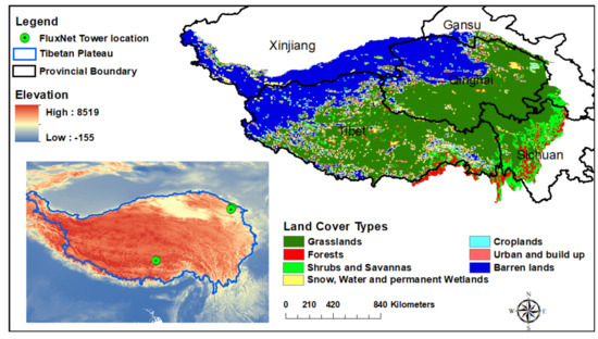
Figure 1.
Administrative and land cover map of the Tibetan Plateau (TP). The boundary of TP is obtained from Yili [43] (DOI:10.3974/geodb.2014.01.12.V1). The land cover map is prepared from MODIS mcd12c1 data; 17 IGBP land cover classes are reclassified and merged into 7 major land covers in TP; insight shows the elevation map of TP using SRTM30 data set (download from https://earthexplorer.usgs.gov/) and locations of FluxNet tower sites.
3. Data and Methods
3.1. CERES Radiation Product
CERES sensors mounted on Terra and Aqua satellites measure top of the atmosphere radiances in three channels; SW (0.3 to 0.5 µm), window (8 to 12 µm) and total (0.3 to 200 µm). These radiances are converted into fluxes using scene type dependent angular distribution models. To provide scene type information, aerosol properties and cloud cover areas, MODIS data is used along with CERES radiances [44,45]. In this study, the CERES Energy Balance and Filled (EBAF) ED4.1 product under clear sky conditions was used for downward shortwave (SW) and longwave (LW) flux at 1-degree spatial resolution. Surface fluxes are computed from CERES_EBAF_TOA flux using Langly Fu-Liou radiative transfer model [45,46]. Uncertainties in the computed downward SW and LW fluxes under clear-sky conditions are 4 Wm−2 and 6 Wm−2, respectively [47]. These data were obtained from the NASA Langley Research Center CERES ordering tool at https://ceres.larc.nasa.gov/.
3.2. MODIS Products
Albedo is a ratio between the reflected and the incident energy in the form of SW radiation. MODIS level 3 daily albedo product (MCD43C3 CMG) at 0.05° spatial resolution was used in this study. This product contains directional hemispherical reflectance (direct or black sky albedo) and bihemispherical reflectance (diffuse or white sky albedo) [48,49]. Black sky albedo was used in this study because a highly correlated value (R = 0.99) between black and white sky albedo provides the liberty to choose either of them. The use of both black and white sky albedo is evident from recent literature [50]. The high quality MODIS albedo product is accurate within 5% at local solar noon [49].
LST and emissivity are two essential parameters for the calculation of upward LW radiation flux. MODIS Terra LST and emissivity monthly product (MOD11C3) at 0.05-degree spatial resolution was used in this study. MODIS LST and emissivity products used a generalized split window algorithm to obtain LST values while the classification based emissivity method is used to obtain emissivity [51,52]. Two daily LST observations are available within MOD11C3, one is at 10:30 AM and the other is at 10:30 PM. The Simplified Merge Scheme (SMS) [53,54] was used to get daily average LST. Collection 6 LST product is validated against various land cover sites and an average standard deviation error is found as less than 0.5K [55]. A study conducted over TP validated MODIS LST and emissivity products using ground based measurements at a semi desert site on western TP [56] Emissivity was obtained from the EMIS31 scientific data set (SDS) of MOD11C3. EMIS31 is based on MODIS band 31 (10,780 to 11,280 nm) and provides more accurate emissivity than other MODIS bands over various land covers [55].
In this study, the MODIS 8-days evapotranspiration and LE product (MOD16A2) at 500 m resolution was used to obtain LE. The product is based on a modified Penman–Monteith method, a complex but well established equation that involves several parameters including saturated water vapor pressure, available energy in the form RN, air density, specific heat capacity of air, aerodynamic resistance, and surface resistance. Mu et al. [57,58] use MODIS remote sensing products of Fraction of Photosynthetically Active Radiation, (FPAR), Leaf Area Index (LAI), land cover, albedo, and NDVI, while tower observations for meteorological data inputs. Obtained results were tested against eddy covariance flux towers from the AmeriFlux network. These towers used the eddy covariance method which is a widely accepted technique to measure energy fluxes. The mean absolute error of daily MODIS ET was observed as 0.33 mm day−1.
For the land cover map of the Tibetan plateau, “MODIS/Terra+Aqua Land Cover Type Yearly L3 Global 0.05-degree CMG” product was used. It provides five different land cover classification schemes, from which the International Geosphere-Biosphere Program (IGBP) scheme was used which classify land into 17 different classes.
MODIS MOD13C2 product provides mean monthly NDVI values at 0.05° spatial resolution. The product computes vegetation indices from MOD09, an atmospherically corrected surface reflectance MODIS product [59,60]. This product was used in this study to quantify vegetation impact on LE.
All MODIS products used in this study were downloaded from NASA’s Level-1 and Atmosphere Archive & Distribution System (LAADS) Distributed Active Archive Center (DAAC) (https://ladsweb.modaps.eosdis.nasa.gov/).
3.3. Reanalysis Data
ERA5 is a long-term reanalysis data set, prepared by ECMWF under Copernicus Climate Change Service (C3S). ERA5 provides more accurate hourly data at a spatial resolution of 31 km compared to the other reanalysis sources [61]. In this study, monthly mean values of net SW, net LW, LE, SH, and air temperature at 0.1° spatial resolution were used. Net SW and net LW were used to compute the RN. The model, Tiled ECMWF Scheme for Surface Exchanges over Land incorporating land surface hydrology (TESSEL) is used in ERA5 land products [62]. These parameters were obtained from https://cds.climate.copernicus.eu/cdsapp#!/home.
For the air temperature at 2 m height, the National Centers for Environmental Prediction (NCEP) reanalysis data were used. NCEP air temperature mean monthly data set is available at 2.5° spatial resolution [63]. The data set has obtained from https://psl.noaa.gov/.
3.4. FluxNet Data
In situ ground observational data was used from the FluxNET2015 data set under the CC-BY-4.0 data policy for validation purposes. Monthly data from three FluxNet stations were used in this study. Site information is summarized in Table 1 [64,65]. This data was downloaded from http://fluxnet.fluxdata.org/. Table 2 provides a summary of all used parameters.

Table 1.
FluxNet data summary. Tier one date of FluxNet2015 data set is used under the CC-BY-4.0 data usage license.
Table 2.
Summary of the satellite, reanalysis data and ground observations used in this study.
3.5. Derivation of SEB from Satellite Data
RN describes the balance between incoming and outgoing radiations in the SW and LW domain. In this study, the RN was derived from Equation (1).
where RS↓ and RL↓ are downward SW and LW radiations respectively. α is the albedo, ɛ is surface emissivity, σ is Stephan–Boltzmann constant (5.67 × 10⁻⁸ Wm−2 · K−4), and T is LST measured in Kelvin. Equation (2) describes the complete equation for the SEB which involves radiative (RN) as well as non-radiative parameters.
where G is ground heat flux. Over large temporal durations, ground heat flux can be ignored since it has a very small range as compared to other energy fluxes. Moreover, it is balanced to zero over the annual cycle [66]. In the next step, SH was calculated by combining Equations (1) and (2) as;
Spatio-temporal, spatial, temporal, and seasonal analyses were performed for RN, SH, and LE from January 2001 to December 2019.
3.6. Comparison Ofmultiple Data Sources
SEB parameters, RN, LE, and SH, were obtained from both satellite and reanalysis data product (ERA5) spatio-temporal, spatial, temporal, and seasonal results from both, satellite and ERA5 data were compared and analyzed to conclude a final result. Next, the temporal trend obtained from LE was compared with the NDVI, and the temporal trend of SH was compared with air temperature and LST.
3.7. Statistical Analysis
To calculate spatio-temporal trends, the Mann–Kendall (M-K) test was used. It is a non-parametric statistical method to establish a monochromatic (increasing or decreasing) trend of any given variable over a defined period [67,68]. The M-K test was performed on mean annual raster images of RN, LE, and SH, to observe any increasing or decreasing trend over the whole TP. Nineteen-years average raster images were produced for spatial analysis. For temporal analysis, Linear Regression (LR) slope test and Sen’s slope test were performed on the decadal scale as well as for the whole study duration. The positive and negative values of these slopes represent increasing or decreasing trends, respectively. For the cross validation of both satellite and ERA5 data, mean bias error (MBE) and mean absolute error (MAE) were checked. These errors describe how closely both data sets are related to each other.
4. Results
4.1. Validation of SEB Parameters
Before the analysis of SEB, first, the accuracy of data as well as method shall be verified. For this purpose, FluxNet tower observations were used. Figure 2 describes the relationship between satellite, ERA5, and in situ ground observations. LR slope, Pearson’s correlation coefficient (r-value), MBE, and MAE were used to check the accuracy of satellite and ERA5 data. Table 3 provides a summary of statistical analyses for the validation of SEB parameters. It is noteworthy that the significance of the correlation values (r-value and LR slope) was obtained at a 95% confidence level. Any value which unsatisfied with this condition is mentioned as insignificant.

Figure 2.
Correlation of satellite and ERA5 data with FluxNet observations. Red line describes the linear regression (LR) slope. Each black dot corresponds to a mean monthly value of surface energy budget (SEB) parameters measured in Wm−2.
Table 3.
Validation statistics of satellite and ERA5 data with respect to FluxNet observations. For LR slope and Pearson’s r; ** describe 99% significance while * describe 95% significance. Without * values are insignificant.
RN observations from satellite and ERA5 data sets are 99% significant with r-values of 0.87 and 0.88, respectively. All four statistical indicators validate the accuracy of the RN from both data sets. LE values are 99% significant and show very less MBE −0.03 and 5.55 Wm−2 and MAE 18.98 and 11.59 Wm−2 for satellite and ERA5 data, respectively. The LR slope value of satellite LE is the only indicator that shows a weak relation with FluxNet observed LE. However, based on the other three statistical parameters, the accuracy of satellite LE is established. For SH, ERA5 observations are validated from 95% significance with 0.81 r-value and 13.19 and 18.92 Wm−2 MBE and MAE, respectively. Satellite observed SH is insignificant (less than 95% significance level). Although the slope value is very high (1.49), yet the low r-value 0.63, and very high MAE 62.85 Wm−2, make this parameter less accurate.
4.2. Spatio-Temporal Analysis
For SEB spatio-temporal trends over TP, the M-K trend test was performed on mean annual raster images of RN, LE and SH obtained from satellite and ERA5 data. The results of M-K tau (τ) values are shown in Figure 3. Positive values (in green and blue) represent increasing trends while negative values (in red and yellow) represent a decreasing trend. RN shows a positive trend in east and southeast TP in both satellite and ERA5 data. Major land covers in these regions are forest and shrub lands as shown in Figure 1. Few pixels in southeast TP show more increasing trends (trend values in between 0.5 to 1) in ERA5 data while such increasing trend is not observable in satellite data. The central regions of TP exhibit a decreasing trend in both data sets. For spatio-temporal trends in the east, southeast and central TP, satellite and ERA5 data are approximately in agreement, but the upper region, the northern part of TP, shows an opposite trend from both data sets. In ERA5 data, these regions show increasing RN trend, with positive M-K τ values, but satellite RN exhibits a decreasing trend (<0 trend values). The major land cover in northern TP is barren land. An overall net positive spatio-temporal trend is dominant in the entire TP.
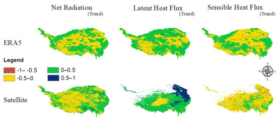
Figure 3.
Spatio-temporal trends of (RN), latent heat flux (LE), and sensible heat flux (SH) from ERA5 and satellite data using M-K τ value. Negative values (red and yellow) correspond to the decreasing trend while positive values (green and blue) correspond to the increasing trend; white regions in satellite LE and SH are the missing values.
LE shows an increasing trend in both data sets, especially satellite LE exhibits a highly increasing trend (M-K τ values approaching 1) in northeast TP. From satellite LE the only decreasing trend is observed in the central region of TP One limitation of the MODIS LE product is that the product does not produce any values for barren lands, thus the northern part of TP cannot be observed from satellite LE data, while ERA5 data covers the whole region. In ERA5 LE, few regions from the northeast and southwest exhibit decreasing trends. The main contradiction is observed in the northeast where satellite LE shows a prominent increasing trend (0.5 to 1 trend value) while ERA5 LE shows a decreasing trend (−0.5 to 0 trend values). Overall a significant increasing trend is observed for LE from both data sets.
The limitation of LE data from MODIS product prolongs to SH as SEB method (Equation (3)) was used to calculate SH. SH shows the only visibly negative trend amongst all SEB parameters. From satellite SH a minor increasing trend in east and central regions of TP is observed, while from ERA5, east, northwest and few central regions of TP show increasing trends. In satellite SH some regions from northeast and southwest show a significant decreasing trend (−1 to −0.5 trend values). In ERA5 SH, such low trend values are not observed.
4.3. Spatial Analysis
For spatial analysis; 19 years mean spatial images were used for RN, LE, and SH from satellite and ERA5 data sets. Figure 4 shows the spatial coverage of all SEB parameters. The upper panel shows the spatial distribution of ERA5 SEB parameters, while the lower panel shows the spatial distribution of satellite SEB parameters. The southeast part of TP exhibits the highest RN values; >150 Wm−2 in satellite data and 90–150 Wm−2 in ERA5 data. In satellite RN, these high values extended towards eastern regions, but in ERA5 RN, the southern regions showed higher values (90–120 Wm−2). Major land covers in the southeast and eastern regions of TP are forests, shrublands, and savannas, while in the southwest part majority of land cover is croplands and grass fields. Northern regions of TP where there are large barren lands as major land cover exhibit least values (from 30 to 60 Wm−2) of RN in satellite and ERA5 data. A contradiction between two data is observed in the west and central regions of TP where ERA5 data show RN as less than 30 and 30–60 Wm−2, respectively, but the same regions from satellite data show the RN as 60 to 120 wm−2.
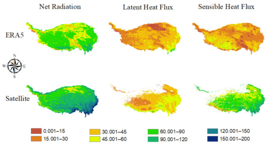
Figure 4.
The spatial trend of RN, LE, and SH from ERA5 and satellite data. Spatial distribution image of each SEB parameter is produced by averaging 19 years mean annual spatial images of the corresponding data (study duration 2001–19). The unit of the legend is Wm−2. White regions in satellite LE and SH are the missing values.
The highest values of LE also belong to southeast regions of TP from both ERA5 (60–90 Wm−2) and satellite (45–60 Wm−2) data sets. This region is rich in forests. In satellite data, the least values which are less than 30 Wm−2 belong to the central and southwest regions. For ERA5 LE, the least values which are less than 15 Wm−2 belong to the northern regions of TP. As mentioned in the above sections, the MODIS LE product has a limitation that the product does not provide values for barren lands, which is abundant in the north TP. One interesting point is that these least values (less than 15 Wm−2) of ERA5 LE are only in the regions which are at the lowest height in the entire TP (as shown in the elevation map in Figure 1). However, there is no scholarly proof of the relationship between LE with altitude. LE has no significant contradiction in spatial patterns between satellite and ERA5 data.
The spatial pattern of SH shows many contradictions in both data sets. The most prominent fact is that satellite SH values are between 45 to 120 Wm−2 (only a few pixels show less than 30 Wm−2) while ERA5 SH values are between 0 to 60 Wm−2. The highest ERA5 SH values (45 to 60 Wm−2) are exhibited in southwest TP, and the highest satellite SH values (90 to 120 Wm-2) are exhibited in southeast TP. A thin strip in the extreme southeast shows the least satellite SH values (less than 30 Wm−2), these pixels in ERA5 SH show the same values. In the northwest, central and southern regions of TP, ERA5 SH exhibit the least values (less than 15 Wm−2), but this trend is not observed in satellite SH.
4.4. Temporal Analysis
For temporal analysis, mean annual aerial averages of RN, LE and SH were computed over the whole TP. On these aerial averages, LR slope and Sen’s slope were computed on a decadal scale and for the whole study duration (2001–19). These slope values are calculated at a 95% confidence level. Figure 5a,c,e shows the ERA5 RN, LE, and SH trends, while Figure 5b,d,f shows the satellite RN, LE, and SH temporal trends. LR slope lines for decadal trends (2001–10 and 2011–19) are shown in blue while temporal trends from 2001–19 are shown in the red line. Table 4 summarizes the temporal trend values of the LR slope and Sen’s slope. Decadal trends of ERA5 RN show negative trends in both LR and Sen’s slope for both decades, but when the temporal trend is computed for complete study duration (2001–19) LR slope and Sen’s slope show increasing trends with the value of 0.01 and 0.02, respectively. For satellite RN, temporal trends for each decade as well as for total study duration show an increasing trend. The overall temporal trend for satellite RN from LR slope and Sen’s slope is 0.01 and 0.03, respectively. Temporal trends of RN from satellite and ERA5 data are in agreement for total study duration and show a nominal increasing trend.
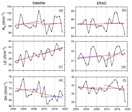
Figure 5.
Temporal variation of RN, LE, and SH based on aerial average over TP. (a,c,e) represent trends observed from satellite data while the (b,d,f) represents trends observed from ERA5 data. Decadal trends are shown in blue and overall temporal trend from 2001–19 is shown in red.
Table 4.
Decadal and total temporal trends of RN, LE, and SH from ERA5 and satellite data sets. LR slope and Sen’s slope are used for temporal trend analysis. ** describe 99% significance while * describe 95% significance. The values after ± are standard errors in LR slope.
For LE, all trends, including the decadal scale and for the total study duration from both data sets show increasing trends in both statistical slopes. However, ERA5 LE shows an overall minor increasing trend with the LR slope and Sen’s slope value 0.03, but for the same duration, satellite LE exhibits 0.25 LR slope and Sen’s slope values which exhibit the prominent increasing trends. For the decadal scale, satellite LE shows the more increasing temporal trend for the second decade (2011–19). This effect is more pronounced in ERA5 LE in which the second decade shows a prominently increasing temporal trend (LR slope and Sen’s slope value 0.15) with respect to the first decade (LR slope and Sen’s slope value 0.02).
SH shows the mixed decadal and overall temporal trends from both data sets. In the LR slope, ERA5 SH shows a continuously decreasing trend for all the temporal durations. Overall, ERA5 LR slope value is −0.016, which exhibits a weak decreasing trend. In the Sen’s slope, the first decade of ERA5 SH shows a decreasing trend while the second decade shows a very weak increasing trend, and for the total duration, Sen’s slope value for ERA5 SH is 0.005, exhibiting a very weak increasing trend. For satellite SH, LR slope values for the first and second decade are 0.04 and 0.02, respectively, and for Sen’s slope, these values are 0.1 and 0.14, respectively. All these four values exhibit a weak but increasing trend. But for the total study duration, both LR slope and Sen’s slope values are −0.18, which exhibit a weak negative trend. Increasing decadal temporal trends but decreasing trends over the longer duration signify the importance of SEB analysis over a longer duration.
4.5. Seasonal Aanalysis
Seasonal averages of RN, LE, and SH from satellite and ERA5 data were computed using aerial averages of TP. Figure 6 shows the seasonal averages of RN, LE, and SH along with the LR slope, and Table 5 summarized the numerical values of computed LR slopes of each trend line marked in Figure 6. For RN, the winter season shows a decreasing trend while the autumn season shows an increasing trend from both satellite and ERA5 observations concluding that RN is reducing in winters and increasing in summers. For the spring and summer (mid-seasons of the year) both data sets exhibit different trends, i.e., in spring, the trend from satellite observations is decreasing while it is increasing in ERA5 observations and vice versa for summer.
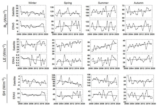
Figure 6.
Seasonal analysis of RN, LE, and SH observed from satellite and ERA5 data. Each value represents the aerial average of the particular SEB parameter for the corresponding season. Straight black lines are LR slopes.
Table 5.
LR slope values of seasonal trends for RN, LE, and SH from satellite and ERA5 data each numerical value represents the corresponding trend line from Figure 6. ** describe 99% significance, while * describes 95% significance. Without * values are insignificant. The values after ± are standard error in LR slope.
For LE, all the seasons from both data sets show prominent increasing trends, except for the winter season from ERA5 data which shows a week decreasing trend, specifically, LE is prominently increasing in the spring and summer months.
Reciprocal to LE, SH exhibit decreasing trends in all four seasons from both data sets except for the spring seasons observed from ERA5 data in which an increasing trend is observed. From the above discussion, it is concluded that both data sets are in agreement for most of the seasonal trends with very few exceptions. Seasonal trends also described that LE is equally increasing while SH is equally decreasing throughout the year from 2001 to 19 over TP. The RN is balanced as it is increasing in half of the year (two seasons) while decreasing for the remaining half year. There is no prominent trend for RN in the overall annual cycle.
4.6. NDVI and LE
The most prominent trend is observed in LE for the temporal, spatial, and spatio-temporal domain. The LE and evapotranspiration are directly related to the vegetation cover of the surface. In this section, the trends of NDVI are analyzed, and the impact of NDVI on LE is observed. Figure 7a describes the spatio-temporal trends of NDVI using M-K τ values. Figure 7b gives the temporal variation of NDVI from mean annual aerial averages over TP. LR slope and Sen’s slope is used to find the temporal trend. The LR and Sen’s slope positive trend values of 0.008 exhibit an increasing temporal trend for NDVI in TP. From the spatio-temporal analysis, the north and northeast regions of TP show the most increasing trends (trend values 0.5 to 1). Other regions exhibit a moderate positive trend (trend values 0 to 0.5) of NDVI. Only a few central regions (with trend values −0.5 to 0) show a negative trend. Here, it is noteworthy that the same central regions of TP exhibit negative trends in LE, as discussed in Section 4.2.
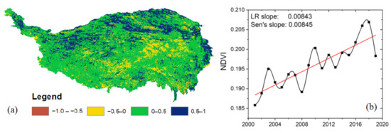
Figure 7.
Normalized Difference Vegetation Index (NDVI)analysis: (a) spatio-temporal analysis of NDVI using M-K τ value (negative values represent decreasing trends while positive value represents increasing value) and (b) temporal analysis (each point represents mean annual aerial average of NDVI over TP). The Red line is the LR slope line which represents a temporal trend.
Figure 8a shows the correlation (r-value) between LE and NDVI. Figure 8b shows the correlation (r-value) between the M-K trend of LE with the M-K trend of NDVI. Random points were observed from both trend images to establish a correlation between LE and NDVI. Only satellite LE is used to find the correlation to avoid sensor calibration factors. A total of 99% of significant correlations are observed at a 95% confidence level. From a significant r-value (0.754) between NDVI and LE, the spatio-temporal and temporal analysis, the argument becomes stronger that NDVI analysis is a useful mechanism to analyze LE.
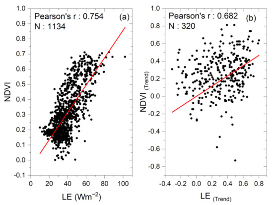
Figure 8.
(a) Correlation between NDVI and satellite LE; both parameters are obtained from MODIS products. Each point represents a random pixel value taken from mean monthly images of NDVI and satellite LE (b) Correlation between NDVI trend and LE trend. A total of 320 random pixels were selected from NDVI and satellite LE spatio-temporal trend images which are produced using the M-K trend test.
4.7. LST, Air Temperature and SH
SH is defined as the heat which can change the temperature without changing the state of matter. Thus, the SH must have a strong relationship with surface and atmospheric temperature. In this section, a correlation is computed between satellite SH with satellite (MODIS) LST and ERA5 SH with the ERA5 air temperature at 2 m height. To avoid any sensor calibration and get a more synchronized correlation, parameters from the same sensors/data sets are selected. Figure 9a shows the correlation r-value between satellite SH and MODIS LST, and Figure 9b shows the r-value between ERA5 SH and ERA5 air temperature. Both correlations are 99% significant at a 95% confidence level. The relation between SH and LST observed from satellite data sources showed a strong positive correlation of 0.763. The correlation between SH and air temperature shows a weak r-value of 0.376. This weak correlation indicates the significance of other factors (such as wind direction, wind speed, and relative humidity) on air temperature.
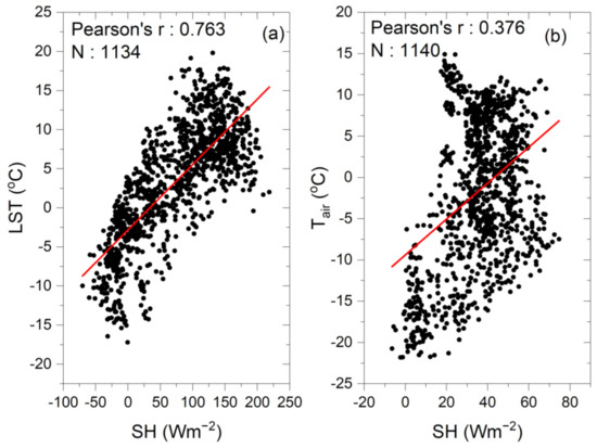
Figure 9.
Correlation between (a) LST obtained from MODIS product and satellite SH. Random pixels were selected from mean monthly images of both parameters; a significant r-value shows the strong correlation between both parameters. (b) Air temperature at 2 m obtained from ERA5 and ERA5 SH. Below-average r-value exhibits that these factors are not closely related to each other.
Figure 10 shows the temporal variation of air temperature obtained from two reanalysis data sets, ERA5 and NCEP. It is observed that air temperature from ERA5 and NCEP shows a positive (increasing) trend with the LR slope value 0.018 and 0.073, respectively, and Sen’s slope value 0.022 and 0.069, respectively. The importance of the factors other than SH can be observed by comparing temporal trends of SH from Figure 5 with the temporal trends of air temperature presented in Figure 10. SH shows a decreasing trend over TP; still, the temporal trend of air temperature is increasing in the same region.
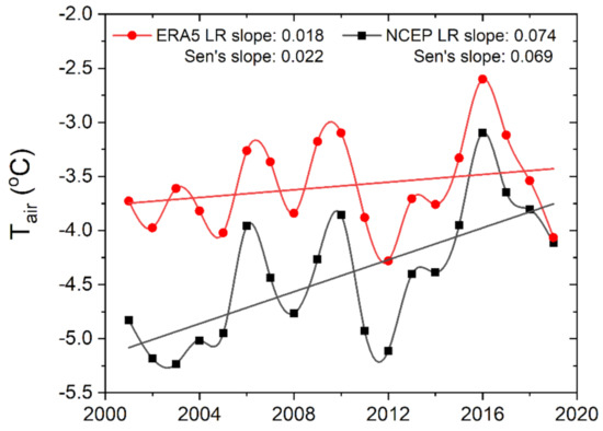
Figure 10.
The temporal trend of air temperature at 2 m height was obtained from ERA5 and NCEP. Each point represents the aerial average of mean annual value over TP. straight lines are LR slope values. Both LR slope and Sen’s slope were computed at a 95% confidence level.
5. Discussions
In this study, two different data sources were used to analyze spatio-temporal trends of RN, LE and SH over TP. the first data source is the satellite data obtained from two different sensors, CERES and MODIS, and the second data source is a reanalysis data product ERA5. In this way, a comparative spatio-temporal analysis was performed on SEB parameters. The first step was to validate the data and method; for this purpose, both data sets were compared with in situ ground measurements from FluxNet tower observations. Four statistical parameters (Pearson’s r, LR slope, MBE, and MAE) were used to validate satellite and ERA5 data. From the results, it is established satellite and ERA5 RN is both valid and reliable with r-values of 0.87 and 0.88, respectively. ERA5 LE resulted in a more accurate LR slope than satellite LE. The LR slope of satellite LE (0.35) is significantly less than the LR slope of ERA5 LE (0.75), but smaller MBE (−0.36 Wm−2) of satellite LE as compared to MBE of ERA5 LE (5.55 Wm−2) shows that over the annual cycle, satellite LE is closer to the ground observations. Satellite SH is the only SEB parameter that shows an insignificant relation with ground observations. High MAE (62.85 Wm−2) and low r-value (0.63) make satellite SH less accurate than ERA5 SH, which has low MAE (18.92 Wm−2) and 95% significant high r-value (0.81). Although satellite SH obtained from CERES and MODIS using Equation (3) is evident from recent literature [15,38,69], in this study, its accuracy is low.
For the cross validation, MBE and MAE were calculated on aerial averages of mean monthly satellite and ERA5 observations. Table 6 presents the summary of statistical error values; here, bias was calculated using satellite—ERA5 observations. Positive MBE and MAE mean that satellite observations are higher than ERA5 observations. LE represents the least MBE and MAE, but MAE for SH is very high (53.91 Wm-2) concluding that satellite SH prominently overestimates ERA5 SH.
Table 6.
Cross validation of SEB parameters. MBE and MAE are calculated from mean monthly observations of RN, LE, and SH observed from satellite and ERA5 data sets. The bias is computed as satellite–ERA5 data, thus the positive values correspond to the higher satellite observations.
Spatio-temporal trends were calculated from M-K trend analysis. For RN, east and southeast regions of TP show the same increasing trends in satellite and ERA5 data sets, but the northern TP shows opposite spatio-temporal trends in both data sets. In the spatial analysis, almost the same pattern was observed that both data sets are in agreement in southeast and eastern TP but the northern TP shows the opposite trends. From Figure 1, it is clear that the majority of land covers in eastern regions of TP are forests, shrubs, and savannas. Moreover, these regions are relatively at low altitudes. Over these land covers, satellite and ERA5 data show similar results. The major land cover in northern TP is barren land; here, both data sets exhibit opposite results. Satellite (MODIS) LE product is the only satellite product that observes evapotranspiration and LE over 109.03 million km2 global vegetated land [57], but the limitation of the product is that it does not observe LE over barren lands. Hence in north TP where the majority of land cover is barren lands, satellite LE is not applicable. In other regions of TP, satellite LE and ERA5 LE are in agreement and exhibit a net increasing trend except for northeast TP, where ERA5 TP shows decreasing spatio-temporal trends. Over northern barren lands, ERA5 LE has the least spatial value between 0 to 15Wm−2. NDVI is an important factor to analyze LE. In Figure 7a, spatio-temporal analyses of NDVI emphasize the spatio-temporal pattern of LE, as the regions with increasing spatio-temporal NDVI trends are those which exhibit spatio-temporal increasing LE trends. For SH, spatio-temporal trends from satellite and ERA5 data show minor increasing trends for east and central TP, but the majority area in TP exhibits decreasing trends. Spatial analysis of SH pronounced the difference in satellite and ERA5 SH as discussed above. Satellite SH observes 60 to 120 Wm−2 in the majority of the regions in TP while ERA5 SH observes 0 to 45 Wm−2 for the same regions. MAE between satellite and ERA5 SH presented in Table 6 points towards this difference. By comparing the MAE of SH from Table 6 with those present in Table 3, it is concluded that satellite SH is overestimated compared to real SH. Our observed spatial pattern of ERA5 LE and SH are identical with Xie et al. [6] observed LE and SH from the ERA-Interim data set. One notable fact is that the east and southeast regions of TP exhibit increasing spatio-temporal trends and higher spatial values for almost all energy fluxes. A possible reason is the land cover change in the area, as it is evident from the literature that in these regions afforestation took place [40,70]. Lands converted to forest from any other land cover exhibit more positive RN and LE [15,50].
For the temporal trends, two different statistical methods, LR slope and Sen’s slope were used in this study. Although LR slope is widely used for time series data, it has a limitation that it is more accurate for the data which best fits on a straight line; moreover, it is more sensitive to the outliers [32]. Sen’s slope is a non-parametric trend method and is not limited to the aforementioned limitations. Thus, by choosing two different trend methods, we eliminate the chances of any bias which may appear because of the statistical method. From these two slopes, temporal trends for each decade (2001–10, 2011–19) and the total study duration (2001–19) were calculated. ERA5 RN shows a minor decreasing decadal trend, but overall study duration exhibits a net increasing trend, while satellite RN consistently shows an increasing trend in each decade and over the whole duration.
LE observed from ERA5 and satellite shows the significant increasing trend in each decade and over the total study duration. Increasing vegetation cover and afforestation is a potential cause for this increase. The argument is strengthening in Figure 7b in which an increasing temporal trend for NDVI is observed. Shen et al. [20] show the increasing vegetation growth in TP using multiple satellite NDVI products and relate this with the evaporative cooling. Our results are in agreement with this study. In Figure 8a, we also established a significant correlation (r-value 0.754) between LE and NDVI in TP.
For ERA5 SH, the LR slope and Sen’s slope exhibit different behavior in the second decade (2011–19) and for the total duration, where LR slope shows a decreasing trend but Sen’s slope shows the increasing trend. The satellite SH shows even more contradictory results; both slopes show increasing trends in the first and second decade, but for the total duration, the trend is decreasing. The different longer trends than decadal trends lead to the conclusion that for the climatic phenomena longer studies are more important and may lead to different results. There is a huge body of literature that observed the SH in TP, some studies use reanalysis data especially for the spring and summer seasons. Almost all studies show the decreasing SH in TP [2,6,30,33,34,35]. Despite a decrease in SH, atmospheric temperature over TP is continuously increasing, resulting in climate warming [1,8,27,29,33]. A weak correlation (r-value 0.376) between SH and air temperature is observed in Figure 9b. Climate warming over TP is observed in Figure 10, in which we show from two reanalysis data sets, ERA5 and NCEP, that mean annual air temperature over TP is temporally increasing from 2001 to 2019.
6. Conclusions
In this study, the spatio-temporal variations of SEB parameters, RN, LE, and SH are analyzed from 2001 to 2019 in the TP using satellite data observed from MODIS and CERES sensors, and reanalysis data from ERA5 data set. After detailed analysis of RN, LE, and SH from satellite and reanalysis data over the TP, we conclude the following results.
- (1)
- After validation from in situ ground observations, RN observed from satellite and ERA5 data are equally reliable and can be used for SEB studies. ERA5 LE is more accurate for monthly analysis, but for annual analysis satellite, LE product (MODIS MOD16A2) can be used as its MAE over a longer duration is less than the MAE of ERA5 LE. Although satellite SH is an efficient alternative over large spatial and longer temporal durations, in the current study it is less accurate than ERA5 SH, which showed better validation statistics in TP. Satellite and ERA5 data observations are in better agreement over forests, savannas and shrub lands, but for barren lands, both observations differ widely.
- (2)
- East and southeast regions of TP exhibit the prominent increasing trend for all SEB parameters, while central regions show decreasing trends. Temporally, a significant increase in LE is observed over TP while a relatively smaller decrease for SH is observed over the same period. RN shows the nominal increasing temporal trend.
- (3)
- NDVI is an important parameter not only for the land cover but also to analyze LE. Over TP, NDVI’s spatial, temporal, and spatio-temporal trends endorsed the trends of LE. Increasing NDVI also enlightens the growing vegetation cover over TP.
- (4)
- SH is an important parameter for the heat cycle, yet it may not solely define the atmospheric temperature trends as SH is decreasing over TP but the air temperature is increasing in the region.
- (5)
- Climate warming and an imbalance between SEB parameters lead towards the thawing of permafrost and snow melting in TP. Being the water head of many important rivers of east and south Asia, any change in the heat cycle of TP enormously affects the whole region. As discussed earlier, TP has a major impact on the Asian monsoon; thus, an increase in LE may alter the Asian monsoon pattern and eventually the whole regional climate.
Author Contributions
Conceptualization, U.M. and S.J.; methodology, U.M., S.J. and M.B.; software, U.M. and M.B.; validation, S.J., M.B. and M.A.A.; formal analysis, U.M. and M.A.A.; investigation, S.J. and W.D.; resources, M.A.A. and H.F.; data curation, U.M. and H.F.; writing—original draft preparation, U.M.; writing—review and editing, S.J., M.B. and W.D.; visualization, U.M. and M.A.A.; supervision, S.J.; project administration, U.M. and S.J.; funding acquisition, S.J. All authors have read and agreed to the published version of the manuscript.
Funding
This study was supported by the National Natural Science Foundation of China (41771069), Jiangsu Province Distinguished Professor Project (Grant No. R2018T20), and Startup Foundation for Introducing Talent of NUIST (Grant No. 2243141801036). The principal author is highly obliged to the China Scholarship Council (CSC) for granting fellowship and providing necessary facilitations.
Data Availability Statement
No new data were created or analyzed in this study. Data sharing is not applicable to this article.
Acknowledgments
The authors would like to acknowledge NASA’s Level-1 and Atmosphere Archive and Distribution System (LAADS) Distributed Active Archive Center (DAAC) for MODIS data, the CERES science team, Copernicus Climate Change Service (C3S) team under European Centre for Medium-range Weather Forecasts for providing ERA5 data and Physical Sciences Laboratory Boulder, Colorado, USA, team for NCEP reanalysis product. We would like to extend our appreciation to the FluxNet tower teams at sites Dangxiong, Haibei shrubland and Haibei alpine Tibet, for providing us valuable tower observations.
Conflicts of Interest
All authors declare that there is not any personal or financial conflicts of interest.
References
- Qiu, J. China: The third pole. Nature 2008, 454, 393–396. [Google Scholar] [CrossRef] [PubMed]
- Duan, A.; Li, F.; Wang, M.; Wu, G. Persistent weakening trend in the spring sensible heat source over the Tibetan Plateau and its impact on the Asian summer monsoon. J. Clim. 2011, 24, 5671–5682. [Google Scholar] [CrossRef]
- Shi, Q.; Liang, S. Surface-sensible and latent heat fluxes over the Tibetan Plateau from ground measurements, reanalysis, and satellite data. Atmos. Chem. Phys. 2014, 14, 5659–5677. [Google Scholar] [CrossRef]
- Duan, J.; Esper, J.; Büntgen, U.; Li, L.; Xoplaki, E.; Zhang, H.; Wang, L.; Fang, Y.; Luterbacher, J. Weakening of annual temperature cycle over the Tibetan Plateau since the 1870s. Nat. Commun. 2017, 8, 1–7. [Google Scholar] [CrossRef] [PubMed]
- Duan, J.; Li, L.; Fang, Y. Seasonal spatial heterogeneity of warming rates on the Tibetan Plateau over the past 30 years. Sci. Rep. 2015, 5, 1–8. [Google Scholar] [CrossRef]
- Xie, J.; Yu, Y.; Li, J.l.; Ge, J.; Liu, C. Comparison of surface sensible and latent heat fluxes over the Tibetan Plateau from reanalysis and observations. Meteorol. Atmos. Phys. 2019, 131, 567–584. [Google Scholar] [CrossRef]
- Immerzeel, W.W.; van Beek, L.P.H.; Bierkens, M.F.P. Climate change will affect the asian water towers. Science 2010, 328, 1382–1385. [Google Scholar] [CrossRef]
- Yao, T.; Xue, Y.; Chen, D.; Chen, F.; Thompson, L.; Cui, P.; Koike, T.; Lau, W.K.; Lettenmaier, D.; Mosbrugger, V.; et al. Recent third pole’s rapid warming accompanies cryospheric melt and water cycle intensification and interactions between monsoon and environment: Multidisciplinary approach with observations, modeling, and analysis. Bull. Am. Meteorol. Soc. 2019, 100, 423–444. [Google Scholar] [CrossRef]
- Wang, X.; Zheng, D.; Shen, Y. Land use change and its driving forces on the Tibetan Plateau during 1990–2000. Catena 2008, 72, 56–66. [Google Scholar] [CrossRef]
- Stephens, G.L.; Li, J.; Wild, M.; Clayson, C.A.; Loeb, N.; Kato, S.; L’ecuyer, T.; Stackhouse, P.W.; Lebsock, M.; Andrews, T. An update on Earth’s energy balance in light of the latest global observations. Nat. Geosci. 2012, 5, 691–696. [Google Scholar] [CrossRef]
- Anderson, R.G.; Canadell, J.G.; Randerson, J.T.; Jackson, R.B.; Hungate, B.A.; Baldocchi, D.D.; Ban-Weiss, G.A.; Bonan, G.B.; Caldeira, K.; Cao, L.; et al. Biophysical considerations in forestry for climate protection. Front. Ecol. Environ. 2011, 9, 174–182. [Google Scholar] [CrossRef]
- Wild, M.; Gilgen, H.; Roesch, A.; Ohmura, A.; Long, C.N.; Dutton, E.G.; Forgan, B.; Kallis, A.; Russak, V.; Tsvetkov, A. From dimming to brightening: Decadal changes in solar radiation at earth’s surface. Science 2005, 308, 847–850. [Google Scholar] [CrossRef] [PubMed]
- Nair, U.S.; Ray, D.K.; Wang, J.; Christopher, S.A.; Lyons, T.J.; Welch, R.M.; Pielke, R.A., Sr. Observational estimates of radiative forcing due to land use change in southwest Australia. J. Geophys. Res. Atmos. 2007, 112, 1–8. [Google Scholar] [CrossRef]
- Bright, R.M.; Davin, E.; O’Halloran, T.; Pongratz, J.; Zhao, K.; Cescatti, A. Local temperature response to land cover and management change driven by non-radiative processes. Nat. Clim. Chang. 2017, 7, 296–302. [Google Scholar] [CrossRef]
- He, T.; Shao, Q.; Cao, W.; Huang, L.; Liu, L. Satellite-observed energy budget change of deforestation in northeastern china and its climate implications. Remote Sens. 2015, 7, 11586–11601. [Google Scholar] [CrossRef]
- Bilal, M.; Nichol, J.E.; Nazeer, M. Validation of Aqua-MODIS C051 and C006 Operational Aerosol Products Using AERONET Measurements over Pakistan. IEEE J. Sel. Top. Appl. Earth Obs. Remote Sens. 2016, 9, 2074–2080. [Google Scholar] [CrossRef]
- Ali, M.A.; Islam, M.M.; Islam, M.N.; Almazroui, M. Investigations of MODIS AOD and cloud properties with CERES sensor based net cloud radiative effect and a NOAA HYSPLIT Model over Bangladesh for the period 2001–2016. Atmos. Res. 2019, 215, 268–283. [Google Scholar] [CrossRef]
- Davin, E.L.; de Noblet-Ducoudre, N. Climatic impact of global-scale Deforestation: Radiative versus nonradiative processes. J. Clim. 2010, 23, 97–112. [Google Scholar] [CrossRef]
- Houspanossian, J.; Nosetto, M.; Jobbágy, E.G. Radiation budget changes with dry forest clearing in temperate Argentina. Glob. Chang. Biol. 2013, 19, 1211–1222. [Google Scholar] [CrossRef]
- Shen, M.; Piao, S.; Jeong, S.J.; Zhou, L.; Zeng, Z.; Ciais, P.; Chen, D.; Huang, M.; Jin, C.S.; Li, L.Z.; et al. Evaporative cooling over the Tibetan Plateau induced by vegetation growth. Proc. Natl. Acad. Sci. USA 2015, 112, 9299–9304. [Google Scholar] [CrossRef]
- Myhre, G.; Samset, B.H.; Hodnebrog, Ø.; Andrews, T.; Boucher, O.; Faluvegi, G.; Fläschner, D.; Forster, P.M.; Kasoar, M.; Kharin, V.; et al. Sensible heat has significantly affected the global hydrological cycle over the historical period. Nat. Commun. 2018, 9, 1–9. [Google Scholar] [CrossRef] [PubMed]
- Ma, Y.; Su, Z.; Koike, T.; Yao, T.; Ishikawa, H.; Ueno, K.I.; Menenti, M. On measuring and remote sensing surface energy partitioning over the Tibetan Plateau-from GAME/Tibet to CAMP/Tibet. Phys. Chem. Earth 2003, 28, 63–74. [Google Scholar] [CrossRef]
- Wang, Y.; Xu, X.; Liu, H.; Li, Y.; Li, Y.; Hu, Z.; Gao, X.; Ma, Y.; Sun, J.; Lenschow, D.H.; et al. Analysis of land surface parameters and turbulence characteristics over the Tibetan Plateau and surrounding region. J. Geophys. Res. 2016, 121, 9540–9560. [Google Scholar] [CrossRef]
- Zhao, P.; Xu, X.; Chen, F.; Guo, X.; Zheng, X.; Liu, L.; Hong, Y.; Li, Y.; La, Z.; Peng, H.; et al. The third atmospheric scientific experiment for understanding the earth–Atmosphere coupled system over the tibetan plateau and its effects. Bull. Am. Meteorol. Soc. 2018, 99, 757–776. [Google Scholar] [CrossRef]
- Xin, Y.F.; Chen, F.; Zhao, P.; Barlage, M.; Blanken, P.; Chen, Y.L.; Chen, B.; Wang, Y.J. Surface energy balance closure at ten sites over the Tibetan plateau. Agric. For. Meteorol. 2018, 259, 317–328. [Google Scholar] [CrossRef]
- Tanaka, K.; Ishikawa, H.; Hayashi, T.; Tamagawa, I.; Yaoming, M. Surface energy budget at Amdo on the Tibetan plateau using GAME/Tibet IOP98 data. J. Meteorol. Soc. Jpn 2001, 79, 505–517. [Google Scholar] [CrossRef]
- You, Q.; Min, J.; Kang, S. Rapid warming in the tibetan plateau from observations and CMIP5 models in recent decades. Int. J. Climatol. 2016, 36, 2660–2670. [Google Scholar] [CrossRef]
- Cai, D.; You, Q.; Fraedrich, K.; Guan, Y. Spatiotemporal temperature variability over the Tibetan Plateau: Altitudinal dependence associated with the global warming hiatus. J. Clim. 2017, 30, 969–984. [Google Scholar] [CrossRef]
- Yan, Y.; You, Q.; Wu, F.; Pepin, N.; Kang, S. Surface mean temperature from the observational stations and multiple reanalyses over the Tibetan Plateau. Clim. Dyn. 2020, 55, 2405–2419. [Google Scholar] [CrossRef]
- Duan, A.; Wang, M.; Lei, Y.; Cui, Y. Trends in summer rainfall over china associated with the Tibetan Plateau sensible heat source during 1980–2008. J. Clim. 2013, 26, 261–275. [Google Scholar] [CrossRef]
- Wang, K.; Ma, Q.; Li, Z.; Wang, J. Decadal variability of surface incident solar radiation over China: Observations, satellite retrievals, and reanalyses. J. Geophys. Res. Atmos. 2015, 120, 6500–6514. [Google Scholar] [CrossRef]
- Zhou, Z.; Wang, L.; Lin, A.; Zhang, M.; Niu, Z. Innovative trend analysis of solar radiation in China during 1962–2015. Renew. Energy 2018, 119, 675–689. [Google Scholar] [CrossRef]
- Yang, K.; Guo, X.F.; Wu, B.Y. Recent trends in surface sensible heat flux on the Tibetan Plateau. Sci. China Earth Sci. 2011, 54, 19–28. [Google Scholar] [CrossRef]
- Zhu, X.Y.; Liu, Y.M.; Wu, G.X. An assessment of summer sensible heat flux on the Tibetan Plateau from eight data sets. Sci. China Earth Sci. 2012, 55, 779–786. [Google Scholar] [CrossRef]
- Zhou, L.T.; Huang, R. Regional differences in surface sensible and latent heat fluxes in China. Theor. Appl. Climatol. 2014, 116, 625–637. [Google Scholar] [CrossRef]
- Liang, S.; Kustas, W.; Schaepman-Strub, G.; Li, X. Impacts of climate change and land use changes on land surface radiation and energy budgets. IEEE J. Sel. Top. Appl. Earth Obs. Remote Sens. 2010, 3, 219–224. [Google Scholar] [CrossRef]
- Liang, S.; Wang, D.; He, T.; Yu, Y. Remote sensing of earth’s energy budget: Synthesis and review. Int. J. Digit. Earth 2019, 12, 737–780. [Google Scholar] [CrossRef]
- Duveiller, G.; Hooker, J.; Cescatti, A. The mark of vegetation change on Earth’s surface energy balance. Nat. Commun. 2018, 9, 679. [Google Scholar] [CrossRef]
- Kandel, R.; Viollier, M. Observation of the Earth’s radiation budget from space. C. R. Geosci. 2010, 342, 286–300. [Google Scholar] [CrossRef]
- Cui, X.; Graf, H.F. Recent land cover changes on the Tibetan Plateau: A review. Clim. Change 2009, 94, 47–61. [Google Scholar] [CrossRef]
- Liu, X.; Chen, B. Climatic warming in the Tibetan Plateau during recent decades. Int. J. Climatol. 2000, 20, 1729–1742. [Google Scholar] [CrossRef]
- Liu, X.; Yin, Z.Y. Sensitivity of East Asian monsoon climate to the uplift of the Tibetan Plateau. Palaeogeogr. Palaeoclimatol. Palaeoecol. 2002, 183, 223–245. [Google Scholar] [CrossRef]
- Yili, Z.; Bingyu, L.; Du, Z. Datasets of the boundary and area of the Tibetan Plateau ZHANG. Acta Geogr. Sin. 2014, 69, 140–143. [Google Scholar]
- Loeb, N.G.; Doelling, D.R.; Wang, H.; Su, W.; Nguyen, C.; Corbett, J.G.; Liang, L.; Mitrescu, C.; Rose, F.G.; Kato, S. Clouds and the Earth’S Radiant Energy System (CERES) Energy Balanced and Filled (EBAF) top-of-atmosphere (TOA) edition-4.0 data product. J. Clim. 2018, 31, 895–918. [Google Scholar] [CrossRef]
- Su, W.; Corbett, J.; Eitzen, Z.; Liang, L. Next-generation angular distribution models for top-of-atmosphere radiative flux calculation from CERES instruments: Methodology. Atmos. Meas. Tech. 2015, 8, 611–632. [Google Scholar] [CrossRef]
- Fu, Q.; Liou, K.N. Parameterization of the radiative properties of cirrus clouds. J. Atmos. Sci. 1993, 50, 2008–2025. [Google Scholar] [CrossRef]
- Kato, S.; Rose, F.G.; Rutan, D.A.; Thorsen, T.J.; Loeb, N.G.; Doelling, D.R.; Huang, X.; Smith, W.L.; Su, W.; Ham, S.H. Surface irradiances of edition 4.0 Clouds and the Earth’s Radiant Energy System (CERES) Energy Balanced and Filled (EBAF) data product. J. Clim. 2018, 31, 4501–4527. [Google Scholar] [CrossRef]
- Schaaf, C.B.; Gao, F.; Strahler, A.H.; Lucht, W.; Li, X.; Tsang, T.; Strugnell, N.C.; Zhang, X.; Jin, Y.; Muller, J.P.; et al. First operational BRDF, albedo nadir reflectance products from MODIS. Remote Sens. Environ. 2002, 83, 135–148. [Google Scholar] [CrossRef]
- Schaaf, C.B.; Liu, J.; Gao, F.; Strahler, A.H. Aqua and terra MODIS albedo and reflectance anisotropy products. In Remote Sensing and Digital Image Processing; Springer: New York, NY, USA,, 2011; Volume 11, pp. 549–561. [Google Scholar]
- Li, Y.; Zhao, M.; Motesharrei, S.; Mu, Q.; Kalnay, E.; Li, S. Local cooling and warming effects of forests based on satellite observations. Nat. Commun. 2015, 6, 1–8. [Google Scholar] [CrossRef]
- Wan, Z. A generalized split-window algorithm for retrieving land-surface temperature from space. IEEE Trans. Geosci. Remote Sens. 1996, 34, 892–905. [Google Scholar]
- Snyder, W.C.; Wan, Z. BRDF models to predict spectral reflectance and emissivity in the thermal infrared. IEEE Trans. Geosci. Remote Sens. 1998, 36, 214–225. [Google Scholar] [CrossRef]
- Bilal, M.; Nichol, J.E.; Wang, L. New customized methods for improvement of the MODIS C6 Dark Target and Deep Blue merged aerosol product. Remote Sens. Environ. 2017, 197, 115–124. [Google Scholar] [CrossRef]
- Bilal, M.; Qiu, Z.; Campbell, J.R.; Spak, S.N.; Shen, X.; Nazeer, M. A new MODIS C6 dark target and Deep Blue merged aerosol product on a 3 km spatial grid. Remote Sens. 2018, 10, 463. [Google Scholar] [CrossRef]
- Wan, Z. New refinements and validation of the collection-6 MODIS land-surface temperature/emissivity product. Remote Sens. Environ. 2014, 140, 36–45. [Google Scholar] [CrossRef]
- Wang, K.; Wan, Z.; Wang, P.; Sparrow, M.; Liu, J.; Haginoya, S. Evaluation and improvement of the MODIS land surface temperature/emissivity products using ground-based measurements at a semi-desert site on the western Tibetan Plateau. Int. J. Remote Sens. 2007, 28, 2549–2565. [Google Scholar] [CrossRef]
- Mu, Q.; Zhao, M.; Running, S.W. Improvements to a MODIS global terrestrial evapotranspiration algorithm. Remote Sens. Environ. 2011, 115, 1781–1800. [Google Scholar] [CrossRef]
- Mu, Q.; Heinsch, F.A.; Zhao, M.; Running, S.W. Development of a global evapotranspiration algorithm based on MODIS and global meteorology data. Remote Sens. Environ. 2007, 111, 519–536. [Google Scholar] [CrossRef]
- Huete, A.; Didan, K.; Miura, T.; Rodriguez, E.P.; Gao, X.; Ferreira, L.G. Overview of the radiometric and biophysical performance of the MODIS vegetation indices. Remote Sens. Environ. 2002, 83, 195–213. [Google Scholar] [CrossRef]
- Vermote, E.F.; el Saleous, N.Z.; Justice, C.O. Atmospheric correction of MODIS data in the visible to middle infrared: First results. Remote Sens. Environ. 2002, 83, 97–111. [Google Scholar] [CrossRef]
- Hersbach, H.; Bell, B.; Berrisford, P.; Hirahara, S.; Horányi, A.; Muñoz-Sabater, J.; Nicolas, J.; Peubey, C.; Radu, R.; Schepers, D.; et al. The ERA5 global reanalysis. Q. J. R. Meteorol. Soc. 2020, 146, 1999–2049. [Google Scholar] [CrossRef]
- Park, S. IFS Doc-Physical Processes; IFS Documentation CY45R1, no. 1. ECMWF, 2018; pp. 1–223. Available online: https://www.ecmwf.int/en/elibrary/18714-part-iv-physical-processes (accessed on 11 January 2021).
- Kalnay, E.; Kanamitsu, M.; Kistler, R.; Collins, W.; Deaven, D.; Gandin, L.; Iredell, M.; Saha, S.; White, G.; Woollen, J.; et al. The NCEP/NCAR 40-year reanalysis project. Bull. Am. Meteorol. Soc. 1996, 77, 437–471. [Google Scholar] [CrossRef]
- Shi, P.; Sun, X.; Xu, L.; Zhang, X.; He, Y.; Zhang, D.; Yu, G. Net ecosystem CO2 exchange and controlling factors in a steppe-Kobresia meadow on the Tibetan Plateau. Sci. China Ser. D Earth Sci. 2006, 49, 207–218. [Google Scholar] [CrossRef]
- Kato, T.; Tang, Y.; Gu, S.; Hirota, M.; Du, M.; Li, Y.; Zhao, X. Temperature and biomass influences on interannual changes in CO2 exchange in an alpine meadow on the Qinghai-Tibetan Plateau. Glob. Chang. Biol. 2006, 12, 1285–1298. [Google Scholar] [CrossRef]
- Bastiaanssen, W.G.M.; Cheema, M.J.M.; Immerzeel, W.W.; Miltenburg, I.J.; Pelgrum, H. Surface energy balance and actual evapotranspiration of the transboundary Indus Basin estimated from satellite measurements and the ETLook model. Water Resour. Res. 2012, 48, 1–16. [Google Scholar] [CrossRef]
- Kendall, M.G. Rank Correlation Methods; Griffin: Oxford, UK, 1948. [Google Scholar]
- Mann, H.B. Nonparametric Tests Against Trend. Econometrica 1945, 13, 245–259. [Google Scholar] [CrossRef]
- Ma, W.; Jia, G.; Zhang, A. Multiple satellite-based analysis reveals complex climate effects of temperate forests and related energy budget. J. Geophys. Res. 2017, 122, 3806–3820. [Google Scholar] [CrossRef]
- Miehe, G.; Miehe, S.; Koch, K.; Will, M. Sacred Forests in Tibet. Mt. Res. Dev. 2003, 23, 324–328. [Google Scholar] [CrossRef]


Publisher’s Note: MDPI stays neutral with regard to jurisdictional claims in published maps and institutional affiliations. |
© 2021 by the authors. Licensee MDPI, Basel, Switzerland. This article is an open access article distributed under the terms and conditions of the Creative Commons Attribution (CC BY) license (http://creativecommons.org/licenses/by/4.0/).