Abstract
Abundant shallow underground brackish water resources could help in alleviating the shortage of fresh water resources and the crisis concerning agricultural water resources in the North China Plain. Improper brackish water irrigation will increase soil salinity and decrease the final yield due to salt stress affecting the crops. Therefore, it is urgent to develop a practical and low-cost method to monitor the soil salinity of brackish irrigation systems. Remotely sensed spectral vegetation indices (SVIs) of crops are promising proxies for indicating the salinity of the surface soil layer. However, there is still a challenge concerning quantitatively correlating SVIs with the salinity of deeper soil layers, in which crop roots are mainly distributed. In this study, a field experiment was conducted to investigate the relationship between SVIs and salinity measurements at four soil depths within six winter wheat plots irrigated using three salinity levels at the Yucheng Comprehensive Experimental Station of the Chinese Academy of Sciences during 2017–2019. The hyperspectral reflectance was measured during the grain-filling stage of winter wheat, since it is more sensitive to soil salinity during this period. The SVIs derived from the observed hyperspectral data of winter wheat were compared with the salinity at four soil depths. The results showed that the optimized SVIs, involving soil salt-sensitive blue, red-edge, and near-infrared wavebands, performed better when retrieving the soil salinity (R2 ≥ 0.58, root mean square error (RMSE) ≤ 0.62 g/L), especially at the 30-cm depth (R2 = 0.81, RMSE = 0.36 g/L). For practical applications, linear or quadratic models based on the screened SVIs in the form of normalized differential vegetation indices (NDVIs) could be used to retrieve soil salinity (R2 ≥ 0.63, RMSE ≤ 0.62 g/L) at all soil depths and then diagnose salt stress in winter wheat. This could provide a practical technique for evaluating regional brackish water irrigation systems.
1. Introduction
The shortage of fresh water is severe in the North China Plain, where 64.7% of the total water use is accounted for by agriculture [1]. Since shallow groundwater brackish water resources (total dissolved solids (TDS) 2–5 g/L) are rich in this region [2], they have been proposed as an alternative irrigation water source to alleviate the water shortage crisis [2,3,4]. Studies have shown that using brackish water irrigation once or twice is feasible for winter wheat during spring when irrigation is necessary in the North China Plain [3,4,5,6]. However, improper brackish water irrigation could increase the soil salinity and cause crop physiological stresses [3,7,8,9,10,11,12,13,14]. Thus, it is crucial to monitor the soil salinity under brackish water irrigation.
Soil salinity along the vertical profile is commonly inhomogeneous because of the vertical movement of water in the soil. To fully understand the degree of salinity stress on crops caused by brackish water irrigation, it is necessary to measure the soil salinity at different depths accurately. Traditional methods for monitoring soil salinity usually require the manual analysis of field soil samples in a laboratory or the installation of in-situ sensors to automatically measure the soil salinity. Neither of these are suitable for regional applications because of their high costs. As remote sensing is a cost-effective, real-time, and non-destructive process with a wide scope, it is commonly used for monitoring crop growth status and soil conditions [6,15,16,17,18,19,20]. Soil salinity has previously been directly derived from the spectra of salinized soil surfaces [21,22,23,24]. However, this method does not work for a salinized soil surface covered by vegetation [21,23,24,25]. Microwave remote sensing can detect the soil surface through the vegetation canopy; however, the working depth is only around 2–5 cm from the surface layer [26]. The above two methods could not quantitatively relate remotely sensed signals with the salinity of deeper soil layers, in which crop roots are mainly distributed. In spectral observations, the soil salinity around the roots of crops is important due to the specific changes in the physiology and morphology of crops caused by environmental stressors [27]. Prior studies have developed various spectral vegetation indices (SVIs) to quantify soil salinity [21,24,28,29,30,31,32,33] (Table 1). Most of them focused on the soil salinity at a target depth, whereas a quantitative investigation concerning SVIs and the soil salinity along the vertical profile has not yet been reported. Besides, the combinations of band types for monitoring soil salinity are different in different studies [21,24,28,29,30,31,32,33]. Therefore, it is necessary to relate soil salinity at different depths and specific band type combinations from crop spectra to better and more quickly grasp the status of soil salt transport.

Table 1.
Summary of the spectral indices for vegetation stress diagnosis 1.
In this study, a field experiment was conducted within six winter wheat plots irrigated using three salinity levels at the Yucheng Comprehensive Experimental Station of the Chinese Academy of Sciences during 2017–2019. According to previous studies, hyperspectral remote sensing with narrow bands can still optimize the band combination and improve the correlations between SVIs and soil salinity [15,24,32,34,35,36]. Therefore, data concerning field hyperspectral observations and salinity measurements at four soil depths during a sensitive stage of winter wheat were used to (1) optimize SVIs for soil salinity at four depths, (2) evaluate the ability of optimized SVI-based retrieval models to estimate the soil salinity at four depths, and then (3) discuss some practical suggestions to quantitatively relate remotely sensed SVIs of crop canopies with saline soil around crop roots.
2. Materials and Methods
2.1. Experimental Site and Design
The field experiment was conducted at the Yucheng Comprehensive Experiment Station (YCES) of the Chinese Academy of Sciences (CAS) in Yucheng, Shandong Province, China (36°57′N, 116°36′E, 28 m a.s.l.), during the growing seasons of winter wheat in 2017–2019 (Figure 1). This site has a semi-humid, temperate, and monsoon climate with an annual average temperature of 13.4 ℃ and an annual total precipitation of 576.7 mm. This climate allows a dominant cropping system of winter wheat and summer maize in the region. The soil in this area is sandy loam (22% sand, 66% silt, and 22% clay), classified as Calcaric Fluvisols according to the FAO-UNESCO system (Food and Agriculture Organization of the United Nations (FAO), 1988), with an average pH of 6.46. The local groundwater depth generally ranges from 1.5 to 4.0 m and has a TDS of approximately 2 g/L. This abundant shallow brackish groundwater resource is widely used to irrigate winter wheat around the experimental site.
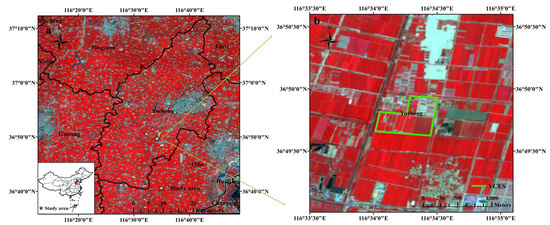
Figure 1.
Satellite images of study area in false color based on Sentinel-2 data from April to June. (a) The position of the Yucheng Comprehensive Experiment Station (YCES) of the Chinese Academy of Sciences (CAS); (b) the experimental area in YCES.
Six plots (5 × 10 m each) were used for the brackish water irrigation experiment (Figure 2). To prevent the movement of water and salt, the plots were separated by a cement wall about 10 cm thick, extending 60 cm deep into the soil and 15 cm above the ground. The experiment consisted of three irrigation treatments, with a replicated plot of each. The treatments included fresh water irrigation (CK, with a TDS of <1 g/L), moderate brackish water irrigation (MS, with a TDS of 3 g/L), and severe brackish water irrigation (SS, with a TDS of 5 g/L). The fresh water was transported from the Yellow River and the experimental brackish water was made of fresh water and sea salt.
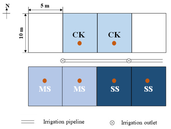
Figure 2.
Schematic diagram of the experimental area of brackish water irrigation. CK is the fresh water irrigation treatment, with a TDS of <1 g/L; MS is the moderate brackish water irrigation treatment, with a TDS of 3 g/L; and SS is the severe brackish water irrigation treatment, with a TDS of 5 g/L. The brown spots refer to the position of the collected soil samples [48].
The experimental plots were sown in 20-cm rows at a density of 225 kg/h with the same local winter wheat variety (JM 22) around October 20th for 3 years. Following the local irrigation system, water with three salinity treatments was used to irrigate the respective plots, with 70 mm used during the jointing stage (around the beginning of April) and 50 mm during the filling stage (around May 11th) of winter wheat (Figure 1). Since there is sufficient rain to leach the salt in the soil from brackish water irrigation in the season of corn growing, it made sure that the brackish water irrigation in the previous year had no effect on the subsequent experiments in the next year. During 2017–2019, the soil moisture was kept at a suitable state, about 62.3–66.7% of the field water capacity. Between the two irrigations, the control of field pests and diseases using pesticides was implemented once. Two fertilizations were completed during the whole growing season of winter wheat. Compound fertilizer (600 kg/ha) was used before sowing and urea (450 kg/ha) was used before the first irrigation. All six experimental plots were under the same field management system, except for the differences in the three irrigation water treatment sources.
2.2. Data Acquisition
During the filling stage, winter wheat leaves grow vigorously and improve their photosynthetic ability. This is a sensitive period for soil moisture and the formation of the final yield. Therefore, in this study, we chose the filling period as the observation period.
In this study, soil salinity data were obtained in a laboratory, using an electrical conductivity meter, as the true data. During the filling stage of winter wheat (around May 15th), soil samples were collected in 10-cm increments down to a depth of 40 cm in each experimental plot, as shown in Figure 2. Thus, 72 soil samples were taken from the six plots during the three years (2017–2019).
Meanwhile, the hyperspectral reflectance of the winter wheat canopy in each plot was measured with a Resonon Pika XC2 hyperspectral imager (Resonon Inc., USA) under cloudless conditions at around 14:00 in the same period (Figure 3a). The Resonon Pika XC2 imaging spectrometer is a compact, high-fidelity instrument used to obtain the complete reflectance image of a plant canopy in the range of 400–1000 nm, with a 1.3-nm spectral resolution (Figure 3b,c). In this study, the hyperspectral imager was mounted on a rocker at a height of 10 m to vertically capture the winter wheat canopy information, facing the sun to avoid the effects of observers and their shadows (Figure 3a). Before acquiring the images, a standard white panel made by Teflon filled the field of view to properly set the exposure and gain, making sure the camera settings were adjusted such that the object under the lighting conditions could be seen. After that, the lens was covered by a cap to remove the dark current noise of the imager from the data. Then, the standard white panel was placed within the view of the imager so that these reflectance observations could be used to correct the reflectance of the whole image. For each experimental plot, one hyperspectral image was obtained during the winter wheat filling period every year (Figure 3b). Therefore, in total, 18 hyperspectral images were obtained during the 3 years (2017–2019).
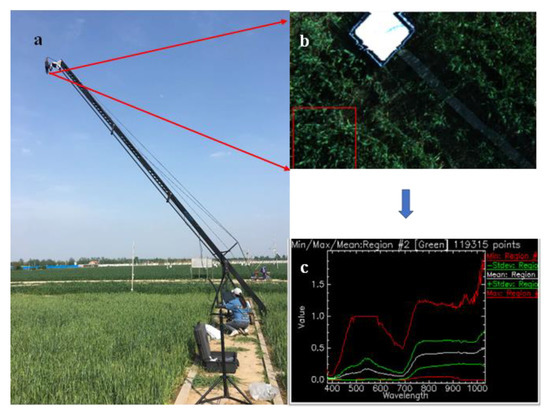
Figure 3.
Acquisition of hyperspectral data in the experimental plots. (a) The instruments for hyperspectral imaging; (b) the reflectance image of the plant canopy; (c) the reflectance curves extracted from the spectral image.
Considering the time cost of calculation and the limited observed area, the minimum distance method was used to extract the pixels of winter wheat from the images before calculating the SVIs, avoiding the effects of weed and soil pixels. Five spectral curves were extracted from each hyperspectral image (Figure 3b,c). The Savitzky-Golay filter, with a step size of 15, was used to reduce the high-frequency noise of the spectral curves and maintain the important spectral curve features [49,50]. Therefore, 5 observed hyperspectral curves with less noise were used to obtain 1 mean curve for each plot, with 18 hyperspectral curves of the 3 treatments obtained during the 3 years.
2.3. Methodology
2.3.1. Screening Soil Salt-Sensitive Wavebands
In this study, hyperspectral observations with narrow bands could help to improve the correlation between spectral vegetation indices and the soil salinity at four soil depths (Figure 4). In order to reduce the number of samples required and save time, two commonly used methods of screening sensitive bands, namely partial least squares regression (PLSR) and stepwise multiple linear regression (SMIR), were used to select the bands sensitive to soil salinity out of all observational bands [51,52]. Firstly, the PLSR analysis was used to relate the multi-colinear and noisy independent variables (reflectance of a given band) to the target-dependent variables (soil salinity at a given soil depth). The regression coefficient (b-coefficient) and variable importance on projection (VIP) from the PLSR analysis were then used to find bands sensitive to soil salinity, as evident when the b-coefficient value is above the standard deviation and the VIP score is greater than 1.0 [53]. Then, SMIR analysis was used to further screen the initially selected bands, considering the combined effects of the bands. Through the SMIR analysis, the independent variables (the reflectance of initially selected bands) were maintained while significantly (p < 0.05) contributing to the target variable of a given soil salinity [54].
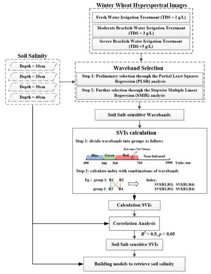
Figure 4.
Flowchart concerning the optimization of spectral vegetation indices (SVIs) and models for retrieving the soil salinity at four depths.
2.3.2. Calculating and Selecting Soil Salt-Sensitive SVIs
The selected soil salt-sensitive wavebands were grouped into three visible regions (blue: 378–500 nm; green: 500–560 nm; red: 600–760 nm), one red-edge region (720–730 nm), and one near-infrared region (760–1000 nm). Following Table 1, the SVIs relating to salt stress consist of six forms: NDVI, ratio vegetation index (RVI), difference vegetation index (DVI), modified simple ratio (MSR), enhanced vegetation index (EVI), modified red-edge normalized differential vegetation index (mNDVI), and plant senescence reflectance index (PSRI). The SVIs were calculated based on these forms, using the selected bands for a given soil depth. If one group consisted of more than one band, the bands in this group were combined with the band/bands in other related groups to calculate the SVIs. When one group did not have any bands, the bands in neighboring groups were suggested for further calculations. Then, correlation analyses were conducted to find SVIs that were more sensitive to soil salinity at a given depth, according to the following coefficients of determination: R2 > 0.5 and p < 0.05. Finally, statistical correlation analysis of data based on steady R2 and root mean square error (RMSE) in different years provided a basis for screening stable SVIs.
2.3.3. Building Models to Correlate Spectral Vegetation Indices with Soil Salinity at Four Depths
Through observations of the soil salinity scatter plots and SVIs, linear and commonly used non-linear (quadratic, logarithmic, or exponential) models were built to retrieve the soil salinity at different depths, with the soil salinity at a given depth being a dependent variable and a given SVI being the independent variable. R2 and root mean square error (RMSE) values were used to quantify the performance of the models. If it was not possible to directly determine the model that should be adopted, the possible models would be tested, with the best model selected based on the highest R2 and lowest RMSE values.
3. Results
3.1. Vertical Distribution of Soil Salinity for Three Brackish Water Irrigation Treatments
The vertical distribution of the soil salinity was different among the three brackish water irrigation treatments and four soil depths (Figure 5). From the 10–40-cm depth, the soil salinity of the <1 g/L TDS treatment increased at a rate of 21.99%, whereas the soil salinity of the TDS treatments at 3 and 5 g/L decreased at rates of 22.27% and 34.46%, respectively. The observed heterogeneous vertical profile of soil salinity suggests that correlating SVIs with soil salinity at different depths could improve our understanding of the effects of salt stress on winter wheat.
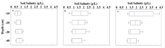
Figure 5.
Vertical distribution of the measured soil salinities for three brackish water irrigation Table 1. g/L (a), 3 g/L (b), and 5 g/L (c).
3.2. Responses of the Hyperspectral Reflectance of the Winter Wheat Canopy to Three Brackish Water Irrigation Treatments
The change in soil salinity may have affected the growth of crops through the root system, which was then reflected in leaf characterization. Comparing the field spectral images of winter wheat with different treatments showed that the winter wheat canopy under the <1 g/L TDS treatment was greener than that under 3 g/L TDS and 5 g/L TDS treatments (Figure 6a–c). However, the physiological response of crops to soil salinity cannot be fully demonstrated by visual differentiation alone.
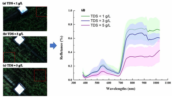
Figure 6.
The progress of extracting the hyperspectral reflectance from winter wheat spectral images. (a–c) are the spectral images of winter wheat canopy with different treatments of TDS <1 g/L (a), 3 g/L (b), and 5 g/L (c); (d) responses of the hyperspectral reflectance of the winter wheat canopy to three brackish water irrigation treatments of a TDS of <1 g/L (green), 3 g/L (blue), and 5 g/L (purple). The color shades along the spectral curves indicate one standard deviation for the spectral reflectance observations in three years.
The observed hyperspectral reflectance of the winter wheat canopy extracted from the images showed obviously different patterns among the three brackish water irrigation treatments (Figure 6). The spectral reflectance curve of the <1 g/L TDS treatment was slightly above that of the 3 g/L TDS treatment, whereas both of them were sharply above that of the 5 g/L TDS treatment, especially within the visible (VIS, 400–760 nm) and near-infrared regions (NIR, 760–1000 nm) (Figure 6d). The decrease in VIS is consistent with the decrease in crop canopy greenness, but the change in spectral information can convey more information about crop physiology. Therefore, the differences in the hyperspectral reflectance among the three brackish water irrigation treatments proved that the salt stress of winter wheat could be diagnosed using hyperspectral observations.
3.3. Optimization of Wavebands and Spectral Vegetation Indices
The b-coefficient and VIP values for each wavelength against the soil salinity at four depths were obtained based on the PLSR analysis, showing how much the spectral bands contribute to retrieving soil salinity (Figure 7 and Figure 8). Then, the sensitive waveband regions were initially selected when the b-coefficient values were above one standard deviation (0.84 for 10-cm depth, 0.14 for 20-cm depth, 0.58 for 30-cm depth, and 0.76 for 40-cm depth) (Figure 7), and the regions were screened according to VIP values that were larger than 1.0 (Figure 8). The wavebands in the blue, green, red-edge, and near-infrared wavelength regions were chosen for the soil depths of 10, 20, 30, and 40 cm, respectively, while the red wavelength region was also chosen for the soil depth of 30 cm (Table 2).
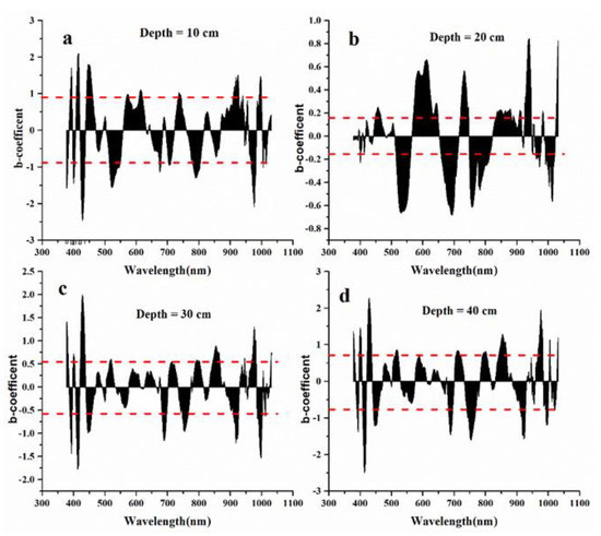
Figure 7.
The b-coefficient values used for the selection of sensitive waveband regions through the relationships with soil salinity at four soil depths. (a) refers to soil depth of 10 cm; (b) refers to soil depth of 20 cm; (c) refers to soil depth of 30 cm; (d) refers to soil depth of 40 cm. The red line refers one standard deviation (0.84 for 10-cm depth, 0.14 for 20-cm depth, 0.58 for 30-cm depth, and 0.76 for 40-cm depth).
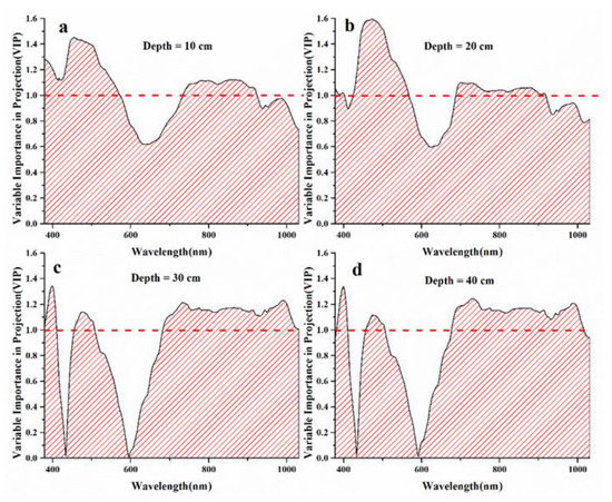
Figure 8.
Variable importance on projection (VIP) values used for the selection of sensitive waveband regions through the relationships with soil salinity at four soil depths. (a) refers to soil depth of 10 cm; (b) refers to soil depth of 20 cm; (c) refers to soil depth of 30 cm; (d) refers to soil depth of 40 cm. The red line refers to VIP = 1.
Table 2.
Waveband regions sensitive to the soil salinity at four depths using the partial least squares regression (PLSR) analysis.
Then, the soil salt-sensitive wavebands for different soil depths were further screened using SMIR analysis (Table 3). For the depth of 10 cm, the bands with central wavelengths of blue (441 nm) and near-infrared (863 nm) were the most sensitive to soil salinity. For the depth of 20 cm, the bands with central wavelengths of blue (446 nm) and red-edge (732 nm) were the most sensitive to soil salinity. As for the depth of 30 cm, the bands with central wavelengths of blue (398 and 454 nm) and near-infrared (760 and 834 nm) were the most sensitive to soil salinity, and for the depth of 40 cm, the bands with central wavelengths of blue (400 and 457 nm) and red-edge (743 nm) were the most sensitive to soil salinity (Table 3). This reveals that blue bands with a wavelength between 398 and 457 nm were sensitive to soil salinity at each depth from 10 to 40 cm, whilst the near-infrared and red-edge bands also help to explain the change in soil salinity.
Table 3.
Waveband regions sensitive to the soil salinity at four depths using stepwise multiple linear regression (SMIR) analysis.
The SVIs, calculated using the selected wavelengths, were correlated with the soil salinity at four depths (Table 4). The results showed that the SVIs in the forms of an NDVI, RVI, DVI, and MSR were sensitive to soil salinity at depths of 10 and 20 cm, whereas the above SVIs as well as those in the forms of an EVI, mNDVI, and PSRI were sensitive to soil salinity at depths of 30 and 40 cm. When the conditions of R2 > 0.5 and p < 0.05 were used to screen the calculated SVIs, which were more sensitive to the soil salinity, it was found that NDVI(441,863), MSR(441,863), and RVI(441,863) were selected for the depth of 10 cm (0.59 ≤ R2 ≤ 0.78); MSR(446,732), NDVI(446,732), and RVI(446,732) were selected for the depth of 20 cm (R2 ≥ 0.63); PSRI(454,760,834), NDVI(454,760), MSR(454,760), NDVI(454,834), and MSR(454,834) were selected for the depth of 30 cm (R2 ≥ 0.66); and NDVI(457,743), RVI(457,743), PSRI(400,457,743), mNDVI(400,457,743), and EVI(400,457,743) were selected for the depth of 40 cm (R2 ≥ 0.58). The screened SVIs are positioned in descending order according to the R2 value for each soil depth. When focusing on the top-ranked SVIs, it was suggested that NDVI and MSR were most sensitive to the soil salinity at depths of 10, 20, and 40 cm, whereas a PSRI involving one blue and two near-infrared bands was most sensitive to the soil salinity at the 30 cm depth.
Table 4.
Statistical correlations between the vegetation indices calculated using the screened wavebands and soil salinity at four depths. The bold section of the table is the selected index along with its R2 and RMSE values.
3.4. Empirical Models for Retrieving the Soil Salinity at Four Soil Depths Using Screened SVIs
Interannual difference analysis of observation data from 2017 to 2019 showed that some SVIs were stable and not affected by climate (Table 5). In addition, it is clearly shown in Table 5 that the selected SVIs performed stably in retrieving the soil salinity at the depth of 10–20 cm. At the depth of 30 cm, despite the performance of other SVIs being disappointing, the relationship between PSRI(454,760,834) and soil salinity had no interannual difference (Table 5). Furthermore, NDVI(457,743), RVI(457,743), and EVI(400,457,743) showed steady close relationships with soil salinity at a 40-cm depth (Table 5).
Table 5.
Statistical correlations of the relationships between the selected SVIs and soil salinity at four depths in 2017–2019. The bold section of the table is the selected index.
Removing unstable SVIs, through visual evaluations of the scatter plots of the screened SVIs and soil salinity at four depths (Figure 9), linear and non-linear empirical models with good performances were proposed (R2 ≥ 0.58, RMSE ≤ 0.62 g/L) (Table 6). The non-linear (quadratic and exponential) models based on MSR(441,863), RVI(441,863), and NDVI(441,863) had similar performances (R2 = 0.78–0.79, RMSE = 0.60–0.62 g/L) at the 10-cm depth. The linear models based on MSR(446,732), RVI(446,732), and NDVI(446,732) had similar performances (R2 = 0.63–0.66, RMSE = 0.44–0.46 g/L) at the 20-cm depth. As for the depth of 30 cm, the quadratic model based on PSRI(454,760,834) had the greatest performance (R2 = 0.81; RMSE = 0.36 g/L). As for the depth of 40 cm, the quadratic models based on NDVI(457,743) and RVI(457,743) had the best performances (R2 = 0.68, RMSE = 0.36–0.37 g/L), whilst the quadratic/linear models based on EVI(400,457,743) had similar performances (R2 = 0.58–0.62, RMSE = 0.40–0.41 g/L). It was also shown that SVIs in the forms of MSR/RVI and NDVI involving the blue and red-edge/near-infrared bands had the closest relationships with the soil salinity at the 10-, 20-, and 40-cm depths, whereas the SVI in the form of a PSRI involving one blue and two near-infrared bands could perform best in relation to the soil salinity at the depth of 30 cm. Then, the soil salinities estimated from the proposed models were compared against the observed soil salinity (Figure 10). The statistical results further indicated the robustness of the proposed empirical models (R2 ≥ 0.58, RMSE ≤ 0.63 g/L). Among all models based on the screened SVIs for all depths, the quadratic model based on the PSRI(454,760,834) performed best when retrieving the soil salinity at the 30-cm depth (R2 = 0.81, RMSE = 0.36 g/L). It was also suggested that the observed spectral information concerning the salt-stressed vegetation canopy was closely related with the salinity at the soil depths where vegetation roots are mainly located.
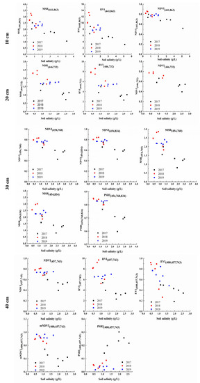
Figure 9.
Scatter plots of the screened SVIs and soil salinity at four depths during 2017–2019.
Table 6.
Proposed models for retrieving the soil salinity at four depths using screened SVIs.
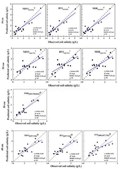
Figure 10.
Comparisons between the observed and predicted soil salinities using the proposed models. L, Q, and E refer to linear, quadratic, and exponential models, respectively.
4. Discussion
4.1. Effect of Soil Salinity on Winter Wheat
Based on the results of this study, it has been shown that the winter wheat spectrum performs well in reflecting the physiological changes of crops under soil salt stress, and it is feasible to detect soil salinity using the crop spectral response. In this study, the spectra of winter wheat leaves under different irrigation treatments showed significant differences (Figure 6). Furthermore, compared with the yield changes of winter wheat in the three years under different treatments (Figure A1), they have similar performances. Soil salinity affects soil water potential. Increases in soil salinity will destroy the balance of water potential inside and outside the crop root cells, affecting crop water absorption. When the soil salt outside the root cells accumulates to a certain degree, it will cause ion toxicity to the cells and destroy their internal structure. These will impact the crop physiological processes such as photosynthesis and transpiration as well as the chlorophyll and cell structure of the leaves, affecting the yield accordingly [24,55,56,57].
Analysis of crop spectra is a method to observe the physiological state of crops from an optical perspective. Previous studies have confirmed that crop spectral indices can be used to observe crop physiological and ecological changes [46,52,56,58,59,60,61]. Therefore, it is theoretically feasible to diagnose soil salinity using leaf spectral analysis.
The decline of the spectral curve under the 3 g/L TDS treatment was slight, indicating that it had little effect on crop physiology (Figure 6). The performance of crop yield also proved the small difference between irrigation under the 3 g/L TDS treatment and fresh water irrigation, with the decline of -0.84–17.67%, which is much lower than the decline under the 5 g/L TDS treatment (5.08–35.40%) (Figure A1). According to previous research, with moderate brackish water irrigation (≤3 g/L TDS), changes in crop physiological state can enhance the ability to adapt to long-term physiological stress without causing damage to the final yield, such as by lowering the stomatal conductance to reduce transpiration [3,9,10,13]. It indicated that brackish water irrigation with reasonable salinity will not cause major damage to crop growth, proving the applicability of brackish water irrigation in the North China Plain.
4.2. Sensitive Bands Related to the Soil Salinity at Different Depths
The results showed that the indices with the combination of blue and red/near-infrared performed well in retrieving the soil salinity at different depths (Table 3 and Table 4). Increase in soil salt around crop roots may decrease the root water absorption, causing a change in the leaf spectrum. Previous studies have suggested that the red-edge and near-infrared bands could help to diagnose salinity stress in crops because of their close relationships with root water absorption [24,55,56,57], which is also shown in our results.
It also shows the effect of visible bands (the blue and red bands) on the retrieval of soil salinity in this study (Table 3). Unlike drought, salt stress also produces ion toxicity and damages cells within the crop. Therefore, the blue and red bands, which can help to quantify the responses of chlorophyll retention, photosynthetic capacity, and internal leaf structure [24,55,56,57], were also selected to estimate the soil salinity at all investigated soil depths. It also highlights the vital role of the blue band in retrieving soil salinity in this study (Table 5), which is different from crop spectral changes under other environmental stresses. It was proven to be highly related to chlorophyll changes, especially chlorophyll b [62].
Although previous research showed that other stressors (i.e., pathogens, herbicides, ozone, and dehydration) could cause similar responses in crop spectral wavebands, there are still differences with soil salt stress (Figure 11). Some stress agents mainly affect the crop water absorption, resulting in great changes in the red-edge and near-infrared wavebands, such as soil drought stress (Figure 11) [15,24,34,55,56,57]. Others can change the physiological structure of crops and the content of chemical substances such as chlorophyll, whose response is mainly concentrated the VIS band regions (Figure 10) [58,59,63,64,65,66]. However, soil salt stress not only affects root water absorption but also produces ion toxicity and damages cells within the crop, whose effects on the crop spectrum are twofold (Figure 10). As this study showed, neither band combination with one signal type region had a strong relationship with soil salinity at any depth, while the combination of the blue and red-edge/near-infrared bands performed well in retrieving the soil salinity.

Figure 11.
Summary of crop spectral sensitive regions under different stresses. The spectral curve was extracted from the winter wheat images of the <1 g/L TDS treatment. The blue box indicates the range of bands sensitive to salt stress proposed in this study; the red boxes indicate the range sensitive to other environmental stresses; refer to [15,24,55,57,64,65,66,67].
4.3. SVIs and Models Selected for Retrieving Soil Salinity
The results showed that the SVIs with soil salt-sensitive bands performed great in retrieving soil salinity for four depths (Table 5 and Table 6). Among them, the form of NDVI is applicable to all soil layers in this study with high accuracy (Table 5). Considering practicality and ease of calculation, SVIs in the form of an NDVI with soil salt-sensitive bands could be used to retrieve the soil salinity at depths from 10 to 40 cm in region scale.
The soil salt content is commonly heterogeneous along a soil profile because of soil water movement [68,69]. However, most studies concerning soil salinity retrievals from SVIs have seldom considered the difference among soil depths [24,32,52,70]. For example, a soil depth of 20 cm is usually assumed to represent the root layer of winter wheat for soil salinity retrievals [24,71]. In this study, the results showed that SVI and SVI-based retrieval models were quite different among four experimental depths (10, 20, 30, and 40 cm) (Table 6). From the screening wavelengths sensitive to soil salinity at each depth, depth-specific SVIs and models were proposed, finding that the retrieval models performed better at deeper soil layers (30–40 cm), especially at the 30-cm depth (R2 = 0.81, RMSE = 0.36 g/L) (Table 6). According to field investigations and previous studies, the root density of winter wheat is relatively high during the filling period, at a depth of 30 cm. In addition, the root system has a stronger water absorption capacity and is more sensitive to salt stress at this depth [72,73,74]. This could explain the closer relationship between the SVIs of the winter wheat canopy and soil salinity at the 30-cm depth. However, for other crops or the same crop during different growing periods, such an optimal depth for diagnosing soil salt stress would change according to the root distribution. Therefore, the differences in the root systems among crop types and growing periods should be considered before diagnosing soil salt stress in crops.
5. Conclusions
In this study, a three-year field experiment was conducted to quantify the relationships between hyperspectral observations of the winter wheat canopy and soil salinity at four soil depths under three brackish water irrigation treatments. The soil salt-sensitive wavebands and SVIs were screened from images based on PLSR and SMIR analyses. Then, empirical models based on the screened SVIs were evaluated for their ability to retrieve the soil salinity at the four soil depths. The results showed that the SVIs involving blue bands along with red-edge/near-infrared bands showed a closer relationship with the soil salinity at all investigated soil depths. Furthermore, the empirical models based on the screened SVIs performed better when retrieving the salinity at the four soil depths (R2 ≥ 0.58, RMSE ≤ 0.62 g/L), especially at the 30-cm depth (R2 = 0.81, RMSE = 0.36 g/L), where winter wheat roots are mainly distributed during the filling period. Considering practicality, it was suggested that SVIs in the form of an NDVI involving the blue bands along with the red-edge/near-infrared bands could be used to retrieve the soil salinity at depths from 10 to 40 cm for practical applications. From this, salt stress on winter wheat could be evaluated by comparing all screened SVIs among the four soil depths. It was also indicted that crop root distributions, which change among crop types and their growing periods, should be considered when remote sensing spectral information is used to diagnose soil salt stress in crops for specific applications.
Author Contributions
Z.S. and F.Z. acquired the funding for hyperspectral and ground measurements. K.Z., Z.S. and F.Z. developed the workflow for this study. K.Z. and W.Z. conducted remote sensing observations and processed the hyperspectral data. J.L. and Z.T. developed a part of the experimental plots with different irrigation treatments. K.Z. and Z.T. measured soil salinity at different depths. K.Z. and Z.S. analyzed the data and wrote the paper. T.Y. and B.L. reviewed and edited the article. All authors have read and agreed to the published version of the manuscript.
Funding
This research was funded by the National Natural Science Foundation of China (31570472), the Strategic Priority Research Program of the Chinese Academy of Sciences (XDA23050102, XDA19040303), the National Key Research and Development Program of China (2017YFC0503805), and Key Projects of the Chinese Academy of Sciences (KJZD-SW-113).
Acknowledgments
The authors would like to give thanks for assistance provided by Yansheng Han, Zhenmin Liu and Hanyou Xie for hyperspectral measurements and to Yulian Liu for assistance with soil salinity measurement in this study.
Conflicts of Interest
The authors declare no conflict of interest.
Appendix A

Figure A1.
Yield changes of the winter wheat under three irrigation treatments in 2017–2019.
References
- Zhang, G.; Lian, Y.; Liu, C.; Yan, M.; Wang, J. Situation and Origin of Water Resources in Short Supply in North China Plain. J. Earth Sci. Environ. 2011, 33, 172–176. [Google Scholar]
- Ma, W.; Cheng, Q.; Li, L.; Yu, Z.; Niu, L.A. Effect of slight saline water irrigation on soil salinity and yield of crop. Trans. CSAE 2010, 26, 73–80. [Google Scholar]
- Wu, Z.; Wang, Q. Response to salt stress aboutnter wheat in Huanghuaihai plain. Agric. Mach. J. 2010, 41, 99–104. [Google Scholar]
- He, K.; Yang, Y.; Yang, Y.; Chen, S.; Hu, Q.; Liu, X.; Gao, F. Hydrus Simulation of Sustainable Brackish Water Irrigation in a Winter Wheat-Summer Maize Rotation System in the North China Plain. Water 2017, 9, 536. [Google Scholar] [CrossRef]
- Wang, H.; Xu, Z.; Pang, G.; Zhang, L.; Wang, X. Effects of Brackish Water Irrigation on Water-salt Distribution and Winter Wheat Growth. J. Soil Water Conserv. 2017, 31, 291–297. [Google Scholar] [CrossRef]
- Liu, X.; Feike, T.; Chen, S.; Shao, L.; Sun, H.; Zhang, X. Effects of saline irrigation on soil salt accumulation and grain yield in the winter wheat-summer maize double cropping system in the low plain of North China. J. Integr. Agric. 2016, 15, 2886–2898. [Google Scholar] [CrossRef]
- Grieve, C.M.; Lesch, S.M.; Maas, E.V.; Francois, L.E. Leaf and spikelet primordia initiation in salt-stressed wheat. Crop Sci. 1993, 33, 1286–1294. [Google Scholar] [CrossRef]
- Grieve, C.M.; Francois, L.E.; Maas, E.V. Salinity affects the timing of phasic development in spring wheat. Crop Sci. 1994, 34, 1544–1549. [Google Scholar] [CrossRef]
- El-Hendawy, S.E.; Hu, Y.; Yakout, G.M.; Awad, A.M.; Hafiz, S.E.; Schmidhalter, U. Evaluating salt tolerance of wheat genotypes using multiple parameters. Eur. J. Agron. 2005, 22, 243–253. [Google Scholar] [CrossRef]
- Chen, S.; Zhang, X.; Shao, L.; Sun, H.; Liu, X. Effect of deficit irrigation with brackish water on growth and yield of winter wheat and summer maize. Chin. J. Eco-Agric. 2011, 19, 579–585. [Google Scholar] [CrossRef]
- Darko, E.; Janda, T.; Majláth, I.; Szopkó, D.; Dulai, S.; Molnár, I.; Türkösi, E.; Molnár-Láng, M. Salt stress response of wheat–barley addition lines carrying chromosomes from the winter barley “Manas”. Euphytica 2014, 203, 491–504. [Google Scholar] [CrossRef]
- Hackl, H.; Hu, Y.; Schmidhalter, U. Evaluating growth platforms and stress scenarios to assess the salt tolerance of wheat plants. Funct. Plant Biol. 2014, 41. [Google Scholar] [CrossRef]
- Yang, T.; Xie, Z.; Yu, Q.; Liu, X. Effects of partial root salt stress on seedling growth and photosynthetic characteristics of winter wheat. Chin. J. Eco-Agric. 2014, 22, 1074–1078. [Google Scholar] [CrossRef]
- Hu, Y.; Hackl, H.; Schmidhalter, U. Comparative performance of spectral and thermographic properties of plants and physiological traits for phenotyping salinity tolerance of wheat cultivars under simulated field conditions. Funct. Plant Biol. 2017, 44, 134. [Google Scholar] [CrossRef] [PubMed]
- Finn, M.P.; Lewis, M.; Bosch, D.D.; Giraldo, M.; Yamamoto, K.; Sullivan, D.G.; Kincaid, R.; Luna, R.; Allam, G.K.; Kvien, C.; et al. Remote Sensing of Soil Moisture Using Airborne Hyperspectral Data. GIScience Remote Sens. 2013, 48, 522–540. [Google Scholar] [CrossRef]
- Li, X.; Tang, Y. Two-dimensional nearest neighbor classification for agricultural remote sensing. Neurocomputing 2014, 142, 182–189. [Google Scholar] [CrossRef]
- Aldabaa, A.; Abdalsatar, A.; Weindorf, D.C.; Chakraborty, S.; Sharma, A.; Li, B. Combination of proximal and remote sensing methods for rapid soil salinity quantification. Geoderma 2015, 239–240, 34–46. [Google Scholar] [CrossRef]
- He, L.; Zhang, H.; Zhang, Y.; Song, X.; Fen, W.; Kang, G.; Wang, C.; Guo, T. Estimating canopy leaf nitrogen concentration in winter wheat based on multi-angular hyperspectral remote sensing. Eur. J. Agron. 2016, 73, 170–185. [Google Scholar] [CrossRef]
- Zhou, X.; Huang, W.; Kong, W.; Ye, H.; Luo, J.; Chen, P. Remote estimation of canopy nitrogen content in winter wheat using airborne hyperspectral reflectance measurements. Adv. Space Res. 2016, 58, 1627–1637. [Google Scholar] [CrossRef]
- El-Hendawy, S.E.; Al-Suhaibani, N.A.; Elsayed, S.; Hassan, W.M.; Dewir, Y.H.; Refay, Y.; Abdella, K.A. Potential of the existing and novel spectral reflectance indices for estimating the leaf water status and grain yield of spring wheat exposed to different irrigation rates. Agric. Water Manag. 2019, 217, 356–373. [Google Scholar] [CrossRef]
- Dehaan, R.L.; Taylor, G.R. Field-derived spectra of salinized soils and vegetation as indicators of irrigation-induced soil salinization. Remote Sens. Environ. 2002, 80, 406–417. [Google Scholar] [CrossRef]
- Metternicht, G.I.; Zinck, J.A. Remote sensing of soil salinity: Potentials and constraints. Remote Sens. Environ. 2003, 85, 1–20. [Google Scholar] [CrossRef]
- Brunner, P.; Li, H.; Kinzelbach, W.; Li, W. Generating soil electrical conductivity maps at regional level by integrating measurements on the ground and remote sensing data. Int. J. Remote Sens. 2007, 28, 3341–3361. [Google Scholar] [CrossRef]
- Zhang, T.; Zeng, S.; Gao, Y.; Ouyang, Z.; Li, B.; Fang, C.; Zhao, B. Using hyperspectral vegetation indices as a proxy to monitor soil salinity. Ecol. Indic. 2011, 11, 1552–1562. [Google Scholar] [CrossRef]
- Spengler, D.; Kuester, T.; Frick, A.; Scheffler, D.; Kaufmann, H. Correcting the influence of vegetation on surface soil moisture indices by using hyperspectral artificial 3D-canopy models. In Remote Sensing for Agriculture, Ecosystems, and Hydrology XV; Neale, C.M.U., Maltese, A., Eds.; SPIE: Bellingham, WA, USA, 2013; Volume 8887. [Google Scholar] [CrossRef]
- Li, B.; Li, Z.; Wei, X. Watershed Soil Moisture Based on Microwave Remote Sensing and Land Surface Model. Remote Sens. Inf. 2007, 96–101. [Google Scholar] [CrossRef]
- Nagler, P.L.; Glenn, E.P.; Huete, A.R. Assessment of spectral vegetation indices for riparian vegetation in the Colorado River delta, Mexico. J. Arid Environ. 2001, 49, 91–110. [Google Scholar] [CrossRef]
- Wiegand, C.L.; Rhoades, J.D.; Escobar, D.E.; Everitt, J.H. Photographic and videographic observations for determining and mapping the response of cotton to soil salinity. Remote Sens. Environ. 1994, 49, 212–223. [Google Scholar] [CrossRef]
- Wang, D.; Wilson, C.; Shannon, M.C. Interpretation of salinity and irrigation effects on soybean canopy reflectance in visible and near-infrared spectrum domain. Int. J. Remote Sens. 2002, 23, 811–824. [Google Scholar] [CrossRef]
- Tilley, D.R.; Ahmed, M.; Son, J.H.; Badrinarayanan, H. Hyperspectral reflectance response of freshwater macrophytes to salinity in a brackish subtropical marsh. J. Environ. Qual. 2007, 36, 780–789. [Google Scholar] [CrossRef]
- Huo, H.; Ni, Z.; Jiang, X.; Zhou, P.; Liu, L. Mineral Mapping and Ore Prospecting with HyMap Data over Eastern Tien Shan, Xinjiang Uyghur Autonomous Region. Remote Sens. 2014, 6, 11829–11851. [Google Scholar] [CrossRef]
- El-Hendawy, S.E.; Hassan, W.M.; Refay, Y.; Schmidhalter, U. On the use of spectral reflectance indices to assess agro-morphological traits of wheat plants grown under simulated saline field conditions. J. Agron. Crop Sci. 2017, 203, 406–428. [Google Scholar] [CrossRef]
- Salah, E.; Waleed, D. Hyperspectral remote sensing to assess the water status, biomass, and yield of maize cultivars under salinity and water stress. Bragantia 2017, 76, 62–72. [Google Scholar] [CrossRef][Green Version]
- Cheng, Y.; Ustin, S.L.; Riaño, D.; Vanderbilt, V.C. Water content estimation from hyperspectral images and MODIS indexes in Southeastern Arizona. Remote Sens. Environ. 2008, 112, 363–374. [Google Scholar] [CrossRef]
- Thenkabail, P.S.; Mariotto, I.; Gumma, M.K.; Middleton, E.M.; Landis, D.R.; Huemmrich, K.F. Selection of Hyperspectral Narrowbands (HNBs) and Composition of Hyperspectral Twoband Vegetation Indices (HVIs) for Biophysical Characterization and Discrimination of Crop Types Using Field Reflectance and Hyperion/EO-1 Data. IEEE J. Sel. Top. Appl. Earth Observ. Remote Sens. 2013, 6, 427–439. [Google Scholar] [CrossRef]
- An, D.; Zhao, G.; Chang, C.; Wang, Z.; Li, P.; Zhang, T.; Jia, J. Hyperspectral field estimation and remote-sensing inversion of salt content in coastal saline soils of the Yellow River Delta. Int. J. Remote Sens. 2016, 37, 455–470. [Google Scholar] [CrossRef]
- Rouse, J.W.; Haas, R.W.; Deering, D.W.; Schell, J.A.; Harlan, J.C. Monitoring the vernal advancement and retrogradation (Greenwave effect) of natural vegetation. In NASA/GSFCT Type III Final Report; NASA: Washington, DC, USA, 1974. [Google Scholar]
- Carlson, T.N.; Gillies, R.R.; Perry, E.M. A method to make use of thermal infrared temperature and NDVI measurements to infer surface soil water content and fractional vegetation cover. Remote Sens. Rev. 1994, 9, 161–173. [Google Scholar] [CrossRef]
- Pearson, R.L.; Miller, L.D. Remote Mapping of Standing Crop Biomass for Estimation of Productivity of the Shortgrass Prairie. In Proceedings of the Eighth International Symposium on Remote Sensing of Environment, Ann Arbor, MI, USA, 2–6 October 1972; Volume 1, pp. 1357–1381. [Google Scholar]
- Jordan, C.F. Derivation of Leaf-Area Index from Quality of Light on the Forest Floor. Ecology 1969, 50, 663–666. [Google Scholar] [CrossRef]
- Huete, A.; Justice, C.; Liu, H. Development of vegetation and soil indices for MODIS-EOS. Remote Sens. Environ. 1994, 49, 224–234. [Google Scholar] [CrossRef]
- Gitelson, A.A.; Merzlyak, M.N.; Grits, Y. Novel algorithms for remote sensing of chlorophyll content in higher plant leaves. In IGARSS ’96—Proceedings of the 1996 International Geoscience and Remote Sensing Symposium: Remote Sensing for a Sustainable Future; IEEE: Lincoln, NE, USA, 1996; Volume I–IV, pp. 2355–2357. [Google Scholar]
- Gamon, J.A.; Penuelas, J.; Field, C.B. A narrow-waveband spectral index that tracks diurnal changes in photosynthetic efficiency. Remote Sens. Environ. 1992, 41, 35–44. [Google Scholar] [CrossRef]
- Gamon, J.A.; Serrano, L.; Surfus, J.S. The photochemical reflectance index: An optical indicator of photosynthetic radiation use efficiency across species, functional types, and nutrient levels. Oecologia 1997, 112, 492–501. [Google Scholar] [CrossRef]
- Fourty, T.; Baret, F.; Jacquemoud, S.; Schmuck, G.; Verdebout, J. Leaf optical properties with explicit description of its biochemical composition: Direct and inverse problems. Remote Sens. Environ. 1996, 56, 104–117. [Google Scholar] [CrossRef]
- Sims, D.A.; Gamon, J.A. Relationships between leaf pigment content and spectral reflectance across a wide range of species, leaf structures and developmental stages. Remote Sens. Environ. 2002, 81, 337–354. [Google Scholar] [CrossRef]
- Merzlyak, M.N.; Gitelson, A.A.; Chivkunova, O.B.; Rakitin, V.Y. Non-destructive optical detection of pigment changes during leaf senescence and fruit ripening. Physiol. Plant. 1999, 106, 135–141. [Google Scholar] [CrossRef]
- Zhu, K.Y.; Sun, Z.G.; Zhao, F.H.; Yang, T.; Tian, Z.R.; Lai, J.B.; Long, B.J.; Li, S.J. Remotely sensed canopy resistance model for analyzing the stomatal behavior of environmentally-stressed winter wheat. ISPRS J. Photogramm. Remote Sens. 2020, 168, 197–207. [Google Scholar] [CrossRef]
- Luo, J.W.; Ying, K.; He, P.; Bai, J. Properties of Savitzky-Golay digital differentiators. Digit. Signal Process. 2005, 15, 122–136. [Google Scholar] [CrossRef]
- Zimmermann, B.; Kohler, A. Optimizing Savitzky-Golay Parameters for Improving Spectral Resolution and Quantification in Infrared Spectroscopy. Appl. Spectrosc. 2013, 67, 892–902. [Google Scholar] [CrossRef] [PubMed]
- Tal, R.; Uri, H.; Maxim, S.; Arnon, K.; Shimon, R. Combining leaf physiology, hyperspectral imaging and partial least squares-regression (PLS-R) for grapevine water status assessment. ISPRS J. Photogramm. Remote Sens. 2015, 109, 88–97. [Google Scholar] [CrossRef]
- El-Hendawy, S.E.; Al-Suhaibani, N.A.; M.Hassan, W.; Dewir, Y.H.; Elsayed, S.; Al-Ashkar, I.; Abdella, K.A.; Schmidhalter, U. Evaluation of wavelengths and spectral reflectance indices for high-throughput assessment of growth, water relations and ion contents of wheat irrigated with saline water. Agric. Water Manag. 2019, 212, 358–377. [Google Scholar] [CrossRef]
- Wold, S.; Sjostrom, M.; Eriksson, L. PLS-regression: A basic tool of chemometrics. Chemom. Intell. Lab. Syst. 2001, 58, 109–130. [Google Scholar] [CrossRef]
- Vasques, G.M.; Grunwald, S.; Sickman, J.O. Comparison of multivariate methods for inferential modeling of soil carbon using visible/near-infrared spectra. Geoderma 2008, 146, 14–25. [Google Scholar] [CrossRef]
- Miller, J.R.; Wu, J.Y.; Boyer, M.G.; Belanger, M.; Hare, E.W. Seasonal patterns in leaf reflectance red-edge characteristics. Int. J. Remote Sens. 1991, 12, 1509–1523. [Google Scholar] [CrossRef]
- Kriston-Vizi, J.; Umeda, M.; Miyamoto, K. Assessment of the water status of mandarin and peach canopies using visible multispectral imagery. Biosyst. Eng. 2008, 100, 338–345. [Google Scholar] [CrossRef]
- Hackl, H.; Mistele, B.; Hu, Y.C.; Schmidhalter, U. Spectral assessments of wheat plants grown in pots and containers under saline conditions. Funct. Plant Biol. 2013, 40, 409–424. [Google Scholar] [CrossRef] [PubMed]
- Goel, P.K.; Prasher, S.O.; Landry, J.A.; Patel, R.M.; Bonnell, R.B.; Viau, A.A.; Miller, J.A. Potential of airborne hyperspectral remote sensing to detect nitrogen deficiency and weed infestation in corn. Comput. Electron. Agric. 2003, 38, 99–124. [Google Scholar] [CrossRef]
- Govind, A.; Bhavanarayana, M.; Kumari, J.; Govind, A. Efficacy of different indices derived from spectral reflectance of wheat for nitrogen stress detection. J. Plant Interact. 2005, 1, 93–105. [Google Scholar] [CrossRef]
- Garrity, S.R.; Eitel, J.U.H.; Vierling, L.A. Disentangling the relationships between plant pigments and the photochemical reflectance index reveals a new approach for remote estimation of carotenoid content. Remote Sens. Environ. 2011, 115, 628–635. [Google Scholar] [CrossRef]
- Feng, W.; Zhang, H.Y.; Zhang, Y.S.; Qi, S.L.; Heng, Y.R.; Guo, B.B.; Ma, D.Y.; Guo, T.C. Remote detection of canopy leaf nitrogen concentration in winter wheat by using water resistance vegetation indices from in-situ hyperspectral data. Field Crop. Res. 2016, 198, 238–246. [Google Scholar] [CrossRef]
- Curran, P.J.; Dungan, J.L.; Peterson, D.L. Estimating the foliar biochemical concentration of leaves with reflectance spectrometry testing the Kokaly and Clark methodologies. Remote Sens. Environ. 2001, 76, 349–359. [Google Scholar] [CrossRef]
- Gomez-Casero, M.T.; Lopez-Granados, F.; Pena-Barragan, J.M.; Jurado-Exposito, M.; Garcia-Torres, L. Assessing nitrogen and potassium deficiencies in olive orchards through discriminant analysis of hyperspectral data. J. Am. Soc. Hortic. Sci. 2007, 132, 611–618. [Google Scholar] [CrossRef]
- Ranjan, R.; Chopra, U.K.; Sahoo, R.N.; Singh, A.K.; Pradhan, S. Assessment of plant nitrogen stress in wheat (Triticum aestivum L.) through hyperspectral indices. Int. J. Remote Sens. 2012, 33, 6342–6360. [Google Scholar] [CrossRef]
- Devadas, R.; Lamb, D.W.; Backhouse, D.; Simpfendorfer, S. Sequential application of hyperspectral indices for delineation of stripe rust infection and nitrogen deficiency in wheat. Precis. Agric. 2015, 16, 477–491. [Google Scholar] [CrossRef]
- Klem, K.; Zahora, J.; Zemek, F.; Trunda, P.; Tuma, I.; Novotna, K.; Hodanova, P.; Rapantova, B.; Hanus, J.; Vavrikova, J.; et al. Interactive effects of water deficit and nitrogen nutrition on winter wheat. Remote sensing methods for their detection. Agric. Water Manag. 2018, 210, 171–184. [Google Scholar] [CrossRef]
- Gosselin, H.; Sagan, V.; Maimaitiyiming, M.; Fishman, J.; Belina, K.; Podleski, A.; Maimaitijiang, M.; Bashir, A.; Balakrishna, J.; Dixon, A. Using Visual Ozone Damage Scores and Spectroscopy to Quantify Soybean Responses to Background Ozone. Remote Sens. 2020, 12, 93. [Google Scholar] [CrossRef]
- Lv, D.; Wang, Q.; Wang, W.; Shao, M. Evaluation of the soil salt distribution characteristics. Acta Pedol. Sin. 2002, 39, 720–725. [Google Scholar]
- Zhang, L.; Wang, Q. Effect of Non-sufficient Irrigation with Saline Water on the Distribution of Water and Salinity in Soil and SWAP Model Simulation. Water Conserv. Irrig. 2015, 7, 32–35. [Google Scholar]
- Prasad, S.; Thenkabail, R.B.S.; De Pauw, E. Evaluation of Narrowband and Broadband Vegetation Indices for Determining Optimal Hyperspectral Wavebands for Agricultural Crop Characterization. Photogramm. Eng. Remote Sens. 2002, 68, 607–622. [Google Scholar]
- Hamzeh, S.; Naseri, A.A.; AlaviPanah, S.K.; Mojaradi, B.; Bartholomeus, H.M.; Clevere, J.G.P.W.; Behzad, M. Estimating salinity stress in sugarcane fields with spaceborne hyperspectral vegetation indices. Int. J. Appl. Earth Obs. Geoinf. 2013, 21, 282–290. [Google Scholar] [CrossRef]
- Xue, Q.; Zhu, Z.; Musick, J.T.; Stewart, B.A.; Dusek, D.A. Root growth and water uptake in winter wheat under deficit irrigation. Plant Soil 2003, 257, 151–161. [Google Scholar] [CrossRef]
- Jha, S.K.; Gao, Y.; Liu, H.; Huang, Z.; Wang, G.; Liang, Y.; Duan, A. Root development and water uptake in winter wheat under different irrigation methods and scheduling for North China. Agric. Water Manag. 2017, 182, 139–150. [Google Scholar] [CrossRef]
- Guo, X.; Sun, X.; Ma, J.; Lei, T.; Zheng, L.; Wang, P. Simulation of the Water Dynamics and Root Water Uptake of Winter Wheat in Irrigation at Different Soil Depths. Water 2018, 10, 1033. [Google Scholar] [CrossRef]
Publisher’s Note: MDPI stays neutral with regard to jurisdictional claims in published maps and institutional affiliations. |
© 2021 by the authors. Licensee MDPI, Basel, Switzerland. This article is an open access article distributed under the terms and conditions of the Creative Commons Attribution (CC BY) license (http://creativecommons.org/licenses/by/4.0/).