Article

Satellite-Based Precipitation Datasets Evaluation Using Gauge Observation and Hydrological Modeling in a Typical Arid Land Watershed of Central Asia

1
State Key Laboratory of Desert and Oasis Ecology, Xinjiang Institute of Ecology and Geography, Chinese Academy of Sciences, Urumqi 830011, China
2
Key Laboratory of GIS & RS Application, Xinjiang Uygur Autonomous Region, Urumqi 830011, China
3
University of Chinese Academy of Sciences, Beijing 100049, China
4
Department of Geography, Ghent University, 9000 Ghent, Belgium
5
Sino-Belgian Joint Laboratory of Geo-Information, Urumqi 830011, China
6
Sino-Belgian Joint Laboratory of Geo-Information, 9000 Ghent, Belgium
7
CAS Research Center of Ecology and Environment in Central Asia, Urumqi 830011, China
*
Author to whom correspondence should be addressed.
Remote Sens. 2021, 13(2), 221; https://doi.org/10.3390/rs13020221
Submission received: 7 December 2020 / Revised: 5 January 2021 / Accepted: 6 January 2021 / Published: 11 January 2021
(This article belongs to the Special Issue Remote Sensing in Hydrology and Water Resources Management)

Abstract

:
Hydrological modeling has always been a challenge in the data-scarce watershed, especially in the areas with complex terrain conditions like the inland river basin in Central Asia. Taking Bosten Lake Basin in Northwest China as an example, the accuracy and the hydrological applicability of satellite-based precipitation datasets were evaluated. The gauge-adjusted version of six widely used datasets was adopted; namely, Precipitation Estimation from Remotely Sensed Information using Artificial Neural Networks–Climate Data Record (CDR), Climate Hazards Group Infrared Precipitation with Stations (CHIRPS), Global Precipitation Measurement Ground Validation National Oceanic and Atmospheric Administration Climate Prediction Center (NOAA CPC) Morphing Technique (CMORPH), Integrated Multi-Satellite Retrievals for GPM (GPM), Global Satellite Mapping of Precipitation (GSMaP), the Tropical Rainfall Measuring Mission (TRMM) and Multi-satellite Precipitation Analysis (TMPA). Seven evaluation indexes were used to compare the station data and satellite datasets, the soil and water assessment tool (SWAT) model, and four indexes were used to evaluate the hydrological performance. The main results were as follows: 1) The GPM and CDR were the best datasets for the daily scale and monthly scale rainfall accuracy evaluations, respectively. 2) The performance of CDR and GPM was more stable than others at different locations in a watershed, and all datasets tended to perform better in the humid regions. 3) All datasets tended to perform better in the summer of a year, while the CDR and CHIRPS performed well in winter compare to other datasets. 4) The raw data of CDR and CMORPH performed better than others in monthly runoff simulations, especially CDR. 5) Integrating the hydrological performance of the uncorrected and corrected data, all datasets have the potential to provide valuable input data in hydrological modeling. This study is expected to provide a reference for the hydrological and meteorological application of satellite precipitation datasets in Central Asia or even the whole temperate zone.

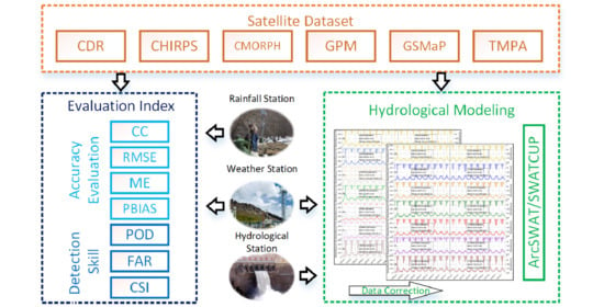
Graphical Abstract

1. Introduction

The importance of precipitation in the water cycle and energy sector has been repeatedly emphasized [1,2,3]. More specifically, the accurate observation of the precipitation process is crucial for modeling the water cycle and forecasting extreme weather events at local, regional, and even global scales [4,5]. However, the understanding of this critical process is limited due to the low coverage of survey stations [6,7]. In many parts of the world, the density of the weather stations is very low or even nonexistent due to technical difficulties or political factors [8,9]. Besides this, the data accessibility of the existing stations is limited as a consequence of the conservative data sharing mechanism, and other reasons such as short record history or deficient data quality, all of which hinder the application of the observed data in hydro-meteorological research [10,11,12].
Fortunately, with the release of the satellite-based precipitation datasets, the gauge observation can be well supplemented in the data-scarce regions, such as arid depopulated zones and alpine areas [13,14]. The launch of the Tropical Rainfall Measuring Mission (TRMM) satellite in 1997 made significant progress in tropical and subtropical satellite precipitation estimation [15,16,17]. Since then, a growing number of high-precision and wide-coverage satellite precipitation datasets have been released. TMPA (TRMM Multi-Satellite Precipitation Analysis) and GPM (Global Precipitation Measurement) are the continuation of TRMM [18,19]. PERSIANN (Precipitation Estimation from Remotely Sensed Information using Artificial Neural Networks) and CHIRP (Climate Hazards Infrared Precipitation) mainly rely on infrared remote sensing technology [20,21]. In addition, there are multi-source datasets such as GSMaP (Global Satellite Mapping of Precipitation) and CMORPH (Climate Prediction Center Morphing Technique) and many others [22,23]. In the field of hydrological modeling, countless studies had proved the applicability of these satellite datasets in many watersheds of the world [24,25,26]. Meanwhile, though, these datasets inevitably showed their uncertainty in the application of different watersheds. In some watershed, the streamflow simulation performance of satellite precipitation is even better than the observed precipitation, e.g., Ziway Lake Basin in Ethiopia and the Adige river basin in Italy [7,9], while performing worse in others, e.g., the Mekong river basin in Southeast Asia and Xiangjiang River Basin in Southeast China [26,27]. As a result, the accuracy and hydrological modeling adaptability evaluation of the satellite datasets in different regions is critical for their application, which is also crucial for the dataset’s improvement. Central Asia is one of the most data-scarce regions around the world due to its complex terrain and underdeveloped economy [28]. For many years, most of the hydrological research in this area has been carried based on limited gauge stations [29,30]. There have been a large number of research cases that refer to the evaluation of satellite precipitation datasets in this area, and Guo et al. reported that the gauge-adjusted versions of four datasets performed better than their unadjusted version, and believed that the GSMaP performed better than others in five Central Asia countries [31]. Gao et al. evaluated the CHIRPS and PERSIANN-CDR in Xinjiang, China, and the results showed that the performance of these two datasets was similar as a whole, but slightly different in the rainfall season and snowfall season [32]. However, the studies on the datasets’ accuracy and hydrological modeling adaptability are rare at the watershed scale, and the comparison of different datasets is even less. Most of the existing limited research was on the application of a single dataset, such as the application of the TMPA in two river basins, including the Hotan River and Syr Darya River [33,34]. At present, several datasets including a new generation of TMPA (GPM) have been applied in many tropical and subtropical basins around the world; thus, evaluating and comparing various satellite precipitation datasets on a watershed scale is meaningful for the hydrological research in Central Asia.
The Bosten Lake Basin is a typical arid inland river basin in Central Asia, where water resources are mainly produced in the high-altitude mountainous areas and evaporate in extremely arid plain areas. In this study, the Bosten Lake Basin was selected as the research area, and six widely used satellite precipitation datasets were adopted for evaluation. The time scale differentiation and the spatial heterogeneity of the datasets were evaluated by multiple indexes, and a distributed hydrological model (soil and water assessment tool) was used to evaluate the dataset’s adaptability in monthly hydrological simulation. For the first time, the encrypted rain gauge station of the local meteorological department was used for satellite datasets evaluation, and the hydrological applicability of the five satellite datasets (only TMPA had already been reported) in the inland river basin of Central Asia has been proven. The main contents include the following: 1. Introduction of the study and the study area (Section 1 and Section 2.1); 2. Data (Section 2.2 and Section 2.3); 3. Methods (Section 2.4 and Section 2.5); 4. Results (Section 3.1 and Section 3.2) and discussion (Section 3.1 and Section 3.2) of the comparison between datasets and observed data; 5. Results (Section 3.3) and discussion (Section 4.3) of the applicability evaluation of the hydrological models; 6. Main conclusions (Section 5). This case study is expected to be meaningful for the hydrological and meteorological application of satellite precipitation datasets in Central Asia, or even the whole temperate zone.

2. Data and Methods

2.1. Study Area

Lake Bosten is a freshwater lake on the northeastern rim of the Tarim Basin, and it is also the largest inland freshwater lake in China. The whole basin is located between latitude 41.25–43.21° N and longitude 82.56–88.20° E, with an area of 4.40 × 10⁴ km2. The main tributaries to the lake are the Kaidu River, Huangshui Ditch, and Qingshui River, of which the Kaidu River accounts for more than 90% of its water inflow. The sources of the Kaidu River are located on the Eren Habirga Mountain of the eastern Tian Shan from where it flows through the Yulduz Basin and the Yanqi Basin into the Bosten Lake. The basin has a large vertical drop with the highest elevation in the upper reaches of 4796 m and the lowest elevation in the downstream of 1037 m.
The grassland and water areas (mostly glaciers) are the primary land-use types in the upper reaches of the basin, accounting for about 61% and 21% of the total upstream area, respectively. In the middle and lower reaches, except for the unused land, the main land-use types are arable land and water area, accounting for about 25% and 15% of the total area, respectively. Like other basins in the arid areas, the Bosten Lake Basin has a clear distinction between dry and wet areas. The average annual precipitation and temperature can reach 504.57 mm and −4.27 °C in a mountainous areas weather station, and the corresponding values in a plain areas station were 67.16 mm and 9.64 °C, respectively. The average annual actual evapotranspiration in the upstream mountain area is about 200 mm, while in the plain area, it can reach 500 mm and 1000 mm in the arable land area and the water area, respectively (Figure 1).

2.2. Observed Data of Ground Stations

The meteorological data include the observation data of 74 rain gauge stations (RG) and 6 national weather (NW) stations. The RG stations’ data were obtained from Xinjiang Meteorological Service (http://xj.cma.gov.cn/) for the period from 2013 to 2019. The NW stations’ data were obtained from China Meteorological Data Service Center (http://data.cma.cn/) for the period from the 1990s to 2019. The monthly streamflow data of the Dashankou hydrological station were collected from the local watershed authority for the period from 1998 to 2019.
Considering the available period of observed data and satellite datasets (Table 1), the observed rainfall (both NW stations and RG stations) and precipitation (only NW stations) were compared with the satellite dataset, and the study periods were set as 2013–2019 and 1998–2019, respectively.
In this study, it is worth noting that spring refers to March, April and May, summer refers to June, July and August, autumn refers to September, October and November, and winter refers to December, January and February. In addition, the watershed is divided by the elevation of 1100 m and 1500 m a.s.l., that is, the upper reaches are higher than 1500 m, the middle reaches are from 1100 m to 1500 m, and the lower reaches are below 1100 m. The division of the watershed is mainly based on the location of the river mountain pass and the boundary of the agricultural irrigation area.

2.3. Satellite Precipitation Datasets

To avoid the influence of different spatial resolutions on the datasets comparison, the dataset with a resolution of 0.25 degrees was selected from different datasets versions as far as possible, and all datasets are the daily data of the gauge-adjusted version (Table 1). To avoid redundancy, the short names in Table 1 were used to refer to each dataset. It is worth noting that the periods in Table 1 refer to the available periods of each dataset, and the periods used in this study are explained in detail in Section 2.2.

2.3.1. CDR

The Precipitation Estimation from Remotely Sensed Information using Artificial Neural Networks–Climate Data Record (CDR) is a dataset that relies heavily on infrared data, and it was converted from a complex PERSIANN algorithm on GridSat-B1 infrared satellite data. The CDR was adjusted using the Global Precipitation Climatology Project (GPCP) monthly product version 2.2 (GPCPv2.2). The dataset was firstly released on 1 June 2014, and was created at a spatial resolution of 0.25 degrees in the latitude band 60S–60N from 1983 to the near-present [35], and the dataset is available on the website of the Center for Hydrometeorology and Remote Sensing (https://chrsdata.eng.uci.edu/), University of California.

2.3.2. CHIRPS

The Climate Hazards Group Infrared Precipitation with Stations (CHIRPS) dataset builds on previous approaches to “smart” interpolation techniques and high-resolution precipitation estimates from long periods of recording, based on infrared cold cloud duration (CCD) observations. The dataset was first released in 2015, and was created at two spatial resolutions of 0.05 degrees and 0.25 degrees in the latitude band 50S–50N from 1981 to the present [36]. The dataset was obtained from the website of the Climate Hazards Center (https://data.chc.ucsb.edu/products/CHIRPS-2.0/), University of California.

2.3.3. CMORPH

The CMORPH is a technique that uses precipitation estimates from low orbiter satellite microwave observations to produce global precipitation analyses at high temporal and spatial resolutions. The dataset version used in this study (CMORPH IFLOODS V1.0 CRT) was released in 2013, which was created at two spatial resolutions of 0.07 degrees and 0.25 degrees in the latitude band 60S–60N from 1998 to the end of 2019 [37], and the dataset was obtained from the file transfer protocol website of NOAA (ftp://ftp.cpc.ncep.noaa.gov/precip/CMORPH_V1.0/).

2.3.4. GPM

The GPM was developed as a continuation and improvement of the TRMM mission, and the Integrated Multi-satellite Retrievals for GPM (IMERG) is an algorithm of GPM which aims to combine multiple types of satellite data including microwave satellite data and infrared satellite data, station gauge data, and others. The latest version (GPM IMERG Final Precipitation L3 V06) was released in March 2019. The temporal coverage is from June 2000 to August 2020, the spatial coverage is in the latitude from 90S to 90N, and the spatial resolution is 0.10 degrees [38]. The dataset is available from the Data and Information Services Center (DISC) of NASA (https://disc.gsfc.nasa.gov/datasets/GPM_3IMERGDF_06/).

2.3.5. GSMaP

The GSMaP is an algorithm of GPM developed by the Japan Aerospace Exploration Agency (JAXA). The main feature of the GSMaP algorithm is the utilization of various attributes derived from the TRMM precipitation radar (TRMM PR) and GPM Dual-Frequency Precipitation Radar Ku Band (GPM DPR Ku). It should be noted that the latest version of the dataset (GSMaP_V7) has not been adopted due to its short time period (2017–present); instead, the GSMaP_V6_Gauge version was adopted in this study [39]. This version was released in April 2016, and was created at two spatial resolutions of 0.10 degrees and 0.25 degrees in the latitude band 60S–60N from March 2000 to the present. The dataset was obtained from the transfer protocol website of the JAXA Earth Observation Research Center (ftp://hokusai.eorc.jaxa.jp).

2.3.6. TMPA

The TMPA is the last dataset of the Tropical Rainfall Measuring Mission (TRMM), and the main feature of the TMPA algorithm is the dense sampling of high-quality microwave data with fill-ins using microwave-calibrated infrared estimates. The dataset version used in this study (TMPA_3B42_daily_V7) was released on May 15, 2016, and was created at a spatial resolution of 0.25 degrees by the DISC of NASA [40]. The temporal coverage is from 1998 to December 30, 2019, the spatial coverage is in the latitude from 50S to 50N, and the data source is the DISC of NASA (https://disc.gsfc.nasa.gov/datasets/TRMM_3B42_Daily_7/).

2.4. The SWAT Model

The soil and water assessment tool (SWAT) is a basin-scale distributed hydrological model. Since the model was jointly developed by the USDA Agricultural Research Service (USDA-ARS) and Texas A&M University in the 1990s [41], it has been applied in many aspects, including the hydrological simulation and the environmental impact evaluation of land-use, land management practices, and climate change. It has also been widely used in the adaptability evaluation of satellite datasets in the hydrological model [9,25,42,43].
The input data of the SWAT model consist of meteorological data and grid data, including terrain data, land-use data, and soil data. The meteorological data are the NW stations and the satellite precipitation datasets mentioned above in Section 2.2 and Section 2.3. The digital elevation model of the Shuttle Radar Topography Mission (SRTM DEM) with a spatial resolution of 90 m was adopted as the terrain data, which can be obtained from the USGS website (https://earthexplorer.usgs.gov/). The soil data are derived from the Harmonized World Soil Database (HWSD), which was created by the Food and Agriculture Organization of the United Nations (FAO) at a spatial resolution of 500 m. Since the land-use types in the upper reaches are almost unchanged due to limited human activity, the land-use data were obtained from the National Cryosphere Desert Data Center (NCDC, http://www.ncdc.ac.cn/) in one single year of 2010, and the spatial resolution is 100 m.
The model setup includes the establishment, calibration, and validation of the model. In the lower reaches of the Kaidu River, there are many diversion canals and drainage ditches that lack observation data, and great human interference factors may affect the comparison in the SWAT model between datasets, and thus the hydrological model is limited to the upstream in this study. Besides this, only the data of three NW stations upstream were used to establish the hydrological model for the following reasons: (1) the lack of snowfall data in RG stations; (2) the significant climate difference between the upper and lower reaches. The monthly hydrological data from 2002 to 2019 was used to verify the simulated streamflow, and the calibration and validation periods were set at 2002–2010 and 2011–2019, respectively. The SUFI-2 algorithm in SWAT-CUP software was used to calibrate the model. After 2000 samplings, the result of the calibration period reached “very good”, and the validation period was “satisfactory” according to a widely used hydrological model guideline [44]; thus the model can be used to evaluate the satellite datasets. The sensitive parameters obtained in the calibration of the watershed were sorted by p-value in the supplementary material (Supplementary Material Table S1).

2.5. Evaluation Indexes and Correction Method

2.5.1. Evaluation Indexes of Datasets Accuracy

To evaluate the ability of each dataset in terms of precipitation estimate, 4 accuracy evaluation indexes were adopted, including the correlation coefficient (CC, optimal value: 1), root mean square error (RMSE, optimal value: 0), mean Error (ME, optimal value: 0), and percent bias (PBIAS, optimal value: 0%). Among them, CC was used to describe the fitting degree between the observed data and satellite datasets, RMSE and ME were used to describe the average difference and average error between the observed data and satellite datasets, and PBIAS was used to reflect the percentage of error.
Three precipitation detection skill indexes were adopted, including probability of detection (POD, optimal value: 1), false alarm ratio (FAR, optimal value: 0), and critical success index (CSI, optimal value: 1). Among them, POD reflects the fraction of correctly estimated times by satellite datasets and actual precipitation times, FAR reflects the fraction of false estimation times and total precipitation times of the satellite datasets, and CSI combines POD and FAR, which can reflect the comprehensive ability of precipitation detection [9]. It should be noted that the above three indexes only judge the occurrence or non-occurrence of precipitation, and have nothing to do with rainfall intensity. The corresponding calculation formulas are given in Equations (1)–(7) [45].
CC   =   i = 1 n [ ( G i G a v e ) · ( S i S a v e ) ] i = 1 n ( G i G a v e ) 2 · i = 1 n ( S i S a v e ) 2
RMSE =   i = 1 n ( S i G i ) 2 n
ME   =   i = 1 n ( S i G i ) n
P B I A S =   i = 1 n ( S i G i ) i = 1 n G i · 100 %
POD =   H H + M
FAR =   F H + F
CSI =   H H + F + M
where G i and G a v e are the observed precipitation and observed average precipitation of the gauge stations, respectively. S i and S a v e are the estimated precipitation and average estimated precipitation of the satellite datasets, respectively. H is the number of hits when the observed value > 0 and estimated value > 0, F is the number of false alarms when the observed value = 0 and the estimated value > 0, and M is the number of misses when the observed value > 0 and the estimated value = 0.

2.5.2. Evaluation Indexes of Hydrological Model

To evaluate the performance of the SWAT model, four widely used indexes were used, including Nash–Sutcliffe efficiency (NSE, optimal value: 1) [46], the coefficient of determination (R2, optimal value: 1), percent bias (PBIAS′, distinguished from PBIAS in Section 2.5.1, optimal value: 0%) and the ratio of mean square error to the standard deviation of the observed data (RSR, optimal value: 0). Among them, NSE indicates the fitting degree between the observed–simulated data point and the 1:1 line, R2 indicates the degree of collinearity between the observed value and simulated value, and RSR is the RMSE normalized by the standard deviation of the observed value. The corresponding calculation formulas are given in Equations (8)–(11) [44].
NSE = 1   i = 1 n ( S I M i O B S i ) 2 i = 1 n ( O B S i O B S a v e ) 2
R 2 = 1   [ i = 1 n ( O B S i O B S a v e ) · ( S I M i S I M a v e ) ] 2 i = 1 n ( O B S i O B S a v e ) 2 · ( S I M i S I M a v e ) 2
P B I A S =   i = 1 n ( S I M i O B S i ) i = 1 n O B S i · 100 %
RSR =   i = 1 n ( O B S i S I M i ) 2 i = 1 n ( O B S i O B S a v e ) 2
where O B S i and O B S a v e are the observed streamflow and average observed streamflow of the hydrological station, respectively. S I M i and S I M a v e are the simulated streamflow and average simulated streamflow by the SWAT model, respectively.

2.5.3. Datasets Correction Method

To improve the performance of the satellite datasets, many complex algorithms (e.g., deep neural network model and dynamic clustered Bayesian averaging) have been developed for the dataset’s inter-calibration, merging, and interpolation [11,47]. However, to avoid the possible impact of excessive correction parameters on the dataset comparison, a relatively straightforward dataset correction method was proposed in this study. The method was inspired by a terrain correction method of precipitation datasets [48]. The deviation degree between satellite precipitation and observed precipitation usually presents a linear distribution at different elevations [49], which can be utilized to enlarge or reduce the satellite data. The corresponding equations are given in Equations (12)–(14).
P s   =   μ · P s = ( a E + b ) · P s
b = i = 1 n [ ( E i E a v e ) · ( P s , i P o , i P s , a v e P o . a v e ) ] i = 1 n [ ( E i E a v e ) 2 ]
a =   P s , a v e P o . a v e b · E a v e
where P s , P s , μ and E are the corrected satellite precipitation, raw satellite precipitation, correction coefficient, and elevation, respectively. P s , i , P o , i and E i are the satellite precipitation, observed precipitation, and elevation at the location of the i th station, respectively. P s , a v e , P o . a v e and E a v e refer to average satellite precipitation, average observed precipitation, and elevation at the locations of all stations.

3. Results

3.1. Comparison Between RG Station Data and Satellite Precipitation Datasets

Since the construction time of the in-situ RG station varies from 2010 to 2012, the evaluation period is selected to be from April to October of each year from 2013 to 2019, which is covered by all in-situ stations and satellite precipitation datasets. Eighty stations with good data quality, including the NW station, were selected for the verification, and the stations that failed to pass the quality control were removed. The quality control processes included climatological limit checks, internal consistency checks, time consistency checks, and missing data checks. Three stations were removed due to excessive missing data. The grid data of satellite precipitation were extracted to points so as to be compared with observed data.

3.1.1. Evaluation Indexes Performance

The results of the evaluation index calculation are presented by box diagrams and table, whereby diagrams are used to show the distribution of 80 stations, and the table is used to show the average value of 80 stations. On the daily scale (Figure 2 and the upper half of Table 2), the GPM dataset had the best CC overall, with an average value of 0.52, and the average CC rankings of six datasets were as follows: GPM > CMORPH > GSMaP > CDR > TMPA > CHIRPS. GPM and CDR performed better than other datasets in terms of RMSE, with an average value of 2.27 mm and 2.38 mm. The performance of all datasets in ME and PBIAS was similar. CMORPH and TMPA overestimated the rainfall with an average ME of 1.08 mm and 0.47 mm, and an average PBIAS of 260.23% and 93.87%, respectively. GPM underestimated the rainfall with an average ME of −0.38 mm and an average PBIAS of −45.08%, while other datasets slightly overestimated by the average ME of 0.25 mm and the PBIAS from 46.96% to 49.70%. Compared with other datasets, CMORPH and TMPA had the most outliers. In terms of rainfall detection, the average PODs of CDR, CMORPH, and GSMaP all exceeded 0.80, but they also had lots of false estimations. In general, GPM exhibited a relatively better rainfall-detecting skill than others on a daily scale.
On the monthly scale (Figure 3 and the lower half of Table 2), the average CC of each dataset was significantly improved, among which CDR and CHIRPS had the most considerable improvement. Therefore, the ranking of average CC also changed to CDR > CHIRPS > GPM > GSMaP > CMORPH > TMPA. In terms of RMSE, all the values were magnified to different degrees, and the average monthly RMSE of all datasets was around 20 mm, except for the immense value of CMORPH and TMPA. For ME and PBIAS, the monthly scale values were very similar to those on the day scale, CMORPH still highly overestimated the rainfall, and GPM was the only underestimated dataset. At the same time, the CDR was still the best dataset overall under these two indexes. The performance in terms of rainfall detection skill was greatly improved over all datasets, almost all months with rainfall events were correctly estimated (average POD: 0.89 for TMPA, 0.99 for GPM, and 1.00 for the other four datasets), the rate of false estimations was significantly reduced (average FAR: 0.16 for CDR, 0.10 for TMPA, and 0.15 for the other four datasets), and the overall rainfall detection skill of all datasets was acceptable (average CSI: all exceeding 0.80).

3.1.2. Influence of Rainfall Intensity on the Evaluation Index

The rainfall distribution has significant regional heterogeneity in the Bosten Lake Basin, and the annual rainfall of each station can vary from 67 mm to 505 mm. Based on the considerations above, it is necessary to evaluate the dataset’s performance under different RG stations sorted by rainfall intensity. In Figure 4, each point represents an observed station. The x-axis indicates the average annual rainfall of the station, and the color and y-axis indicate the performance of different datasets at different station locations under different indexes. At the stations with a higher annual rainfall, the fitting degrees of all satellite datasets with the observed data were greater (Figure 4a), and there was a significant positive correlation (p-value < 0.01) between the annual rainfall and the CC, among which CDR and GSMaP had the strongest correlation. Except for CMORPH, the RMSE of other datasets increased with the increase in rainfall intensity (Figure 4b). The performances of ME and PBIAS were similar, and all satellite datasets were more likely to be underestimated at the stations with more rainfall (Figure 4c,d). As the results of three rainfall detection indexes showed, in the areas with higher annual rainfall, both the numbers of hits and misses had increased, while the number of false alarms decreased noticeably. The PODs of CMORPH and GPM showed a decreasing trend, for the reason that the misses increase more than the growth of the hits as the annual rainfall intensifies, while the PODs of CHIRPS and TMPA showed a decreasing trend due to the opposite situation (Figure 4e). Besides this, the FAR was negatively correlated (p-value <0.01 for all datasets) with rainfall intensity (Figure 4f), and CSI was positively correlated (p-value <0.01 for all datasets) with rainfall intensity (Figure 4g). On the monthly scale, the relationship between evaluation indexes and rainfall intensity is similar to that of the daily scale.

3.1.3. Spatial Distribution of Datasets Performance

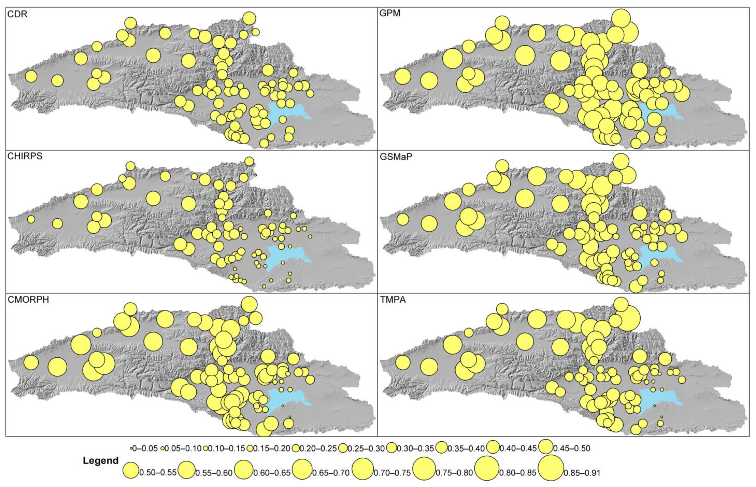
To further understand the performances of different datasets in different regions of the basin, the daily data were selected for evaluation due to their more significant spatial variability compared with monthly data, and the CC and ME were adopted as evaluation indexes. In Figure 5, the larger the yellow circle is, the stronger the correlation between the satellite datasets and the observed data is. As the results are shown, the CC of CDR is not high (varies from 0.22 to 0.43), but its stability is the best in different regions of the basin, which was consistent with the result in the box plot (Figure 2a). The CC level of the CHIRPS dataset is the lowest in the whole basin (average 0.29), and the spatial differentiation is considerable. The excellent performance points of CHIRPS are mainly distributed in the upper high-altitude area and the valley area near the mountain pass of the river (CC is about 0.30–0.55), while the worse points are mainly distributed in the lower reaches of the basin, especially around the lake (CC below 0.25). CMORPH was the second best dataset on CC (average 0.43), which has an even spatial distribution, and only a few low values appear around the lake downstream. GPM was the best dataset in terms of CC performance, both in terms of numerical value (average 0.52) and spatial distribution, and the CC of GPM could be maintained at a high level even in the downstream(about 0.40–0.50 around the lake). The CC performance of GSMaP (average 0.40) was similar to that of CMORPH in the upstream, but in the middle and lower reaches, the CC of GSMaP performed more weakly than CMORPH except for in the area around the lake. The TMPA dataset has greatly uneven spatial distribution in terms of CC, and it performed well in the upstream mountainous regions (the average CC is 0.54 when elevation is above 1500 m), but not well in the lower reaches (the average CC is 0.28 when elevation is below 1100 m).
Compared with CC, the regional characteristics in spatial distribution presented by ME were more prominent. In Figure 6, the blue point means underestimation while the red point means overestimation, and the darker the color, the stronger the underestimation (overestimation). All datasets underestimated rainfall to varying degrees in the upstream, while in the middle and lower reaches, all datasets overestimated rainfall to varying degrees, except for GPM and TMPA (Figure 6). The ME of the CDR in the whole basin was the smallest (average 0.02 mm), the underestimation in the upstream and overestimation in the downstream by CDR were both slight except for a few points, and the ME values were −0.28 mm and 0.14 mm for elevation above 1500 m and below 1500 m, respectively. The ME of CHIRPS showed great uncertainty in the upstream area, which varied greatly even between adjacent regions. The CHIRPS was the only dataset that overestimated the upstream rainfall. Besides this, CHIRPS overestimated greatly in the middle reaches from 1100 m to 1500 m above sea level (average 0.23 mm, the second largest in this region, after CMORPH). For the CMORPH, its significant overestimation in the whole basin was due to the enormous errors in the middle and lower reaches, especially around the lake (ME reaches 3.19 mm when elevation is between 1045 m and 1060 m). However, like other datasets, CMORPH still underestimated the rainfall by the ME of −0.37 mm in the upper reaches. The excessive underestimation in the upper reaches makes GPM the only underestimated dataset for the whole basin (Figure 6 GPM, Figure 2c,d), but if we ignore the upstream area, the performance of GPM in the middle and lower reaches is the best in all datasets (−0.11 mm when elevation is lower than 1500 m). The ME distribution of GSMaP was similar to that of CDR with the uniform spatial distribution and concentrated numerical distribution, while the difference was that the GSMaP had more outliers (Figure 6 GSMaP and Figure 2c). The ME distribution of TMPA was similar to that of GPM, with the same great underestimation in the upstream and the same good performance in the midstream, except for the fact that TMPA overestimated rainfall at several points around the lake (average 0.62 mm from 1045 m to 1060 m a.s.l.).

3.2. Annual and Interannual Performance of Satellite Precipitation Datasets

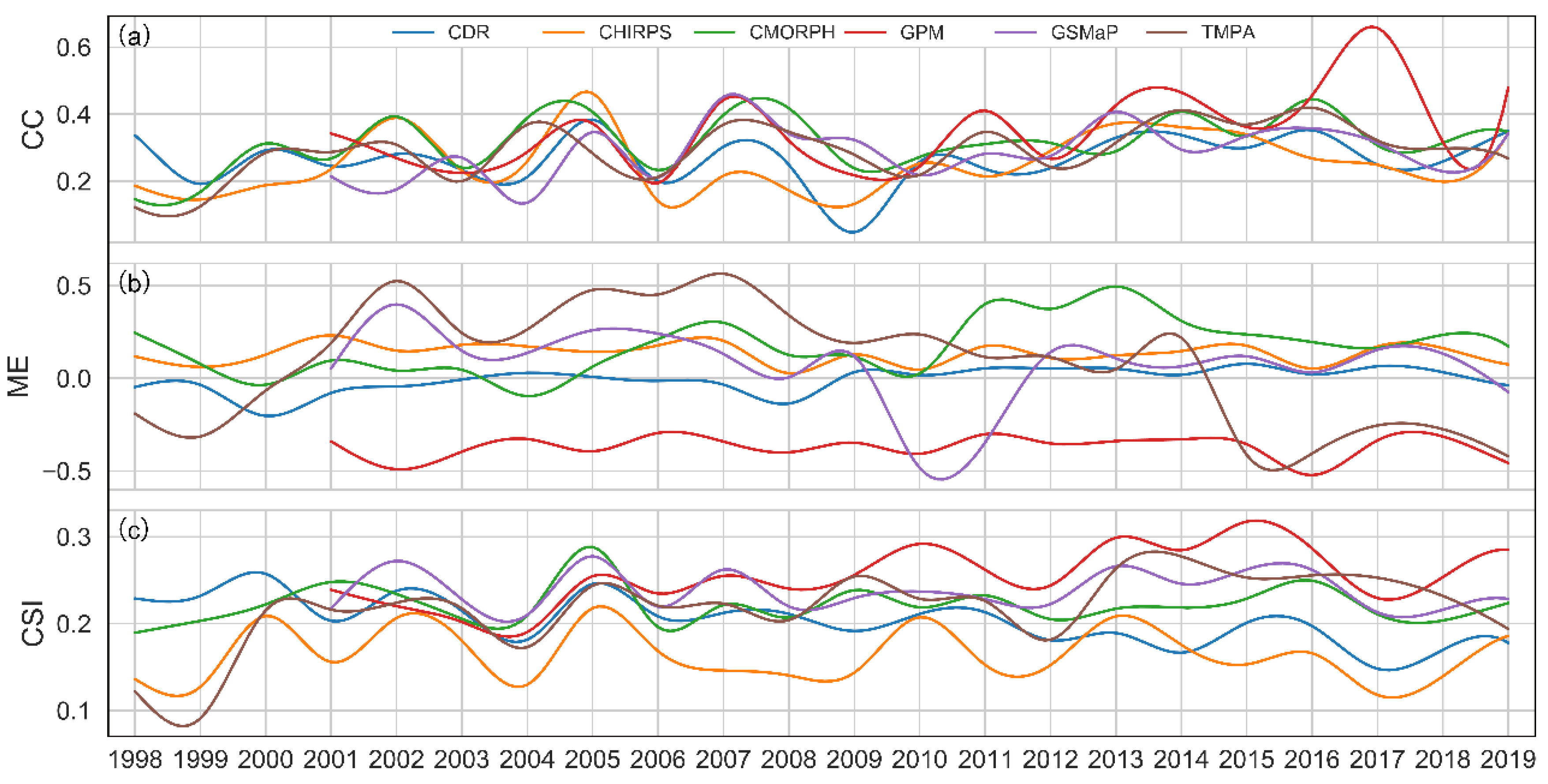
The CC, ME, and CSI were selected to evaluate the performances of different datasets in different months of the year, and the daily precipitation data of six NW stations were adopted, for the reason that there are no observed data from November to March of the next year at the RG stations. The same three indexes were also selected to evaluate the multi-year performance of each dataset; similarly, the data of six NW stations were adopted because of the short construction history (since 2010) of RG stations, and the evaluation period was chosen as from 1998 to 2019, covering all datasets as much as possible.

3.2.1. Performance Variation in Different Months

The monthly distribution of CC (Figure 7a) showed that all datasets performed best in summer (average 0.25 from June to August of all datasets), similarly poorly in spring and autumn (average 0.13), and worst in winter (average 0.03). The CC performance of CDR and CHIRPS was the most uniform among each month. In winter, CHIRPS and CDR were the first and second best datasets, respectively (CDR was 0.07, CHIRPS was 0.09, while all other datasets were less than 0.03). The performances of CMORPH and GSMaP were similar, their CC value was close in each month, and their best two CC values both appeared in July and August. GPM is the best-performing dataset from a year-round perspective. Moreover, the GPM dataset clearly showed better fit degrees compared to other datasets from March to October (CC average 0.28, while the highest of others was 0.18), and the TMPA was the worst dataset in terms of the performance of CC (the average CC of TMPA was only 0.03 except in summer).
In terms of the ME (Figure 7b), the GPM was still the only dataset that underestimated precipitation throughout the year (average 0.40 mm), especially in the summer (average 1.04 mm). The two datasets with the most apparent overestimation were still CMORPH and CHIRPS. Still, the magnitude of their overestimation was smaller compared with RG station data (0.17 mm for CMORPH and 0.13 mm for CHIRPS). The CDR and GSMaP were the two best datasets in terms of ME performance, and the precipitation was underestimated by them at average values of −0.23 mm and −0.11 mm in summer, and overestimated by them at average values of 0.07 mm and 0.19 mm in other seasons, respectively. On the contrary, for TMPA, the precipitation was overestimated by 0.52 mm in summer and underestimated by −0.07 mm in other seasons, respectively. The performances of each dataset in terms of CSI were similar (Figure 7c); they all tended to hit more precipitation events from April to September of the year, and among them, the CHIRPS dataset performed the worst in summer and the best in winter of all datasets.

3.2.2. Trend of Datasets Performance Over the Years

In spite of the volatility, all the datasets showed an upward trend in terms of CC (Figure 8a), with the ascending trend ranking of GPM > TMPA > GSMaP > CMORPH > CHIRPS > CDR, and the corresponding linear rising rates were 0.10/10a (p-value = 0.01), 0.06/10a (p-value = 0.01), 0.06/10a (p-value = 0.05), 0.05/10a (p-value = 0.05), 0.04/10a (p-value = 0.10) and 0.02/10a (p-value > 0.10). Among them, the CDR was still the most stable dataset in the multi-year evaluation, and the CC values of CDR were all in the range of 0.2 to 0.4, except in 2009. On the contrary, the CHIRPS was not stable; although its overall trend was increasing, it had declined for five consecutive years from 2013 to 2018. The CC of GPM reached 0.66 in 2017, which was the highest among all datasets in all years.
Most of the datasets had a stable ME over the years (Figure 8b), among which CDR had the smallest error in almost every year (within ±0.10 mm/d in 20 of 22 years). CHIRPS showed a slight overestimation every year, with a maximum of 0.23 mm/d (2001), while GPM showed a serious underestimation every year, ranging from −0.29 mm/d to −0.52 mm/d. Except for the abnormally high value in 2002 and the unusually low values in 2010 and 2011, the GSMaP dataset slightly overestimated the precipitation in the remaining 16 years. In contrast, CMORPH and TMPA were not as stable as the other four datasets. The CMORPH was the most overestimated dataset in every year from 2011, although the mean error was not evident before. As for the TMPA, it changed from the most underestimated dataset before 2000 to the most overestimated dataset from 2002 to 2010, and then dropped to the same underestimation level as GPM after 2015. The performance of each dataset changed little in terms of CSI over the years (Figure 8c), among which the CDR declinined at the rate of 0.03/10a; GPM and TMPA increased at the rate of 0.04/10a. Furthermore, the change rates of other datasets were less than 0.01/10a and did not pass the significance test.

3.2.3. Multi-year Variation of Correlation Coefficient in Each Month

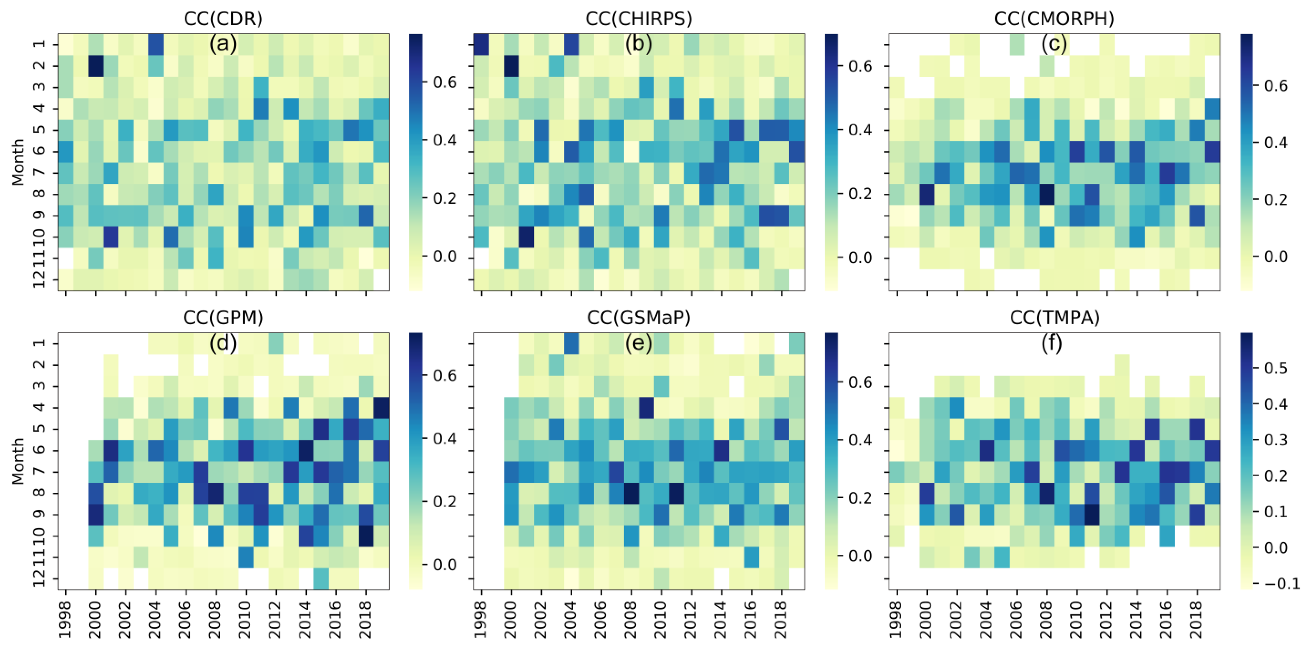
Given the apparent change in CC compared to other indexes, a more detailed multi-year monthly change analysis was carried out on CC. The performances of all datasets in each month since 1998 are shown by the heat map (Figure 9). Each grid in the graph represents a month; the darker the color, the greater the correlation coefficient. The CDR and CHIRPS showed homogeneity on CC multi-year performance, and they filled every month except the no-precipitation months of November 1998 and December 2019 in the NW station (Figure 9 CDR, CHIRPS). In April and May, the CDR dataset showed a significant linear upward trend, with the average rising rates of 0.10/10a and 0.09/10a on CC, respectively, while in December, the CC decreased by 0.10/10a. Similarly, the CC of CHIRPS had risen by 0.14/10a and 0.09/10a in May and June, respectively, and showed a downward trend in January by −0.11/10a. Except for the months mentioned above, there was no obvious trend in the other months of these two datasets.
CMORPH and TMPA were the two worst-performing datasets in winter, especially TMPA, which hit only one month with winter precipitation in 22 years (Figure 9. CMORPH, TMPA). In May, June, and September, the CMORPH dataset showed an obvious upward trend, with an average increase rate of 0.13/10a, 0.11/10a, and 0.14/10a in terms of CC, respectively. The TMPA dataset showed an increasing trend in June, July, and September, and the increasing rates were 0.11/10a, 0.12/10a, and 0.10/10a, respectively, and in other months, neither the TMPA or the CMORPH showed an obvious upward or downward trend.
The data of GPM and GSMaP both started after 2000 (Figure 9 GPM, GSMaP). Among them, the GPM dataset had the most obvious rising trend in all datasets, and its rising rates reached 0.13/10a, 0.22/10a, and 0.17/10a in April, May, and October, respectively. Although the average increasing rate of the GSMaP in all months was 0.06/10a, ranking second in all six datasets, its upward trend was significant only in June by 0.10/10a.

3.3. Performance in Hydrological Simulations

Considering the climate variation in different regions of the arid basin, the rainfall station data cannot be used for the hydrological modeling of the whole year. Therefore, the input meteorological data of the SWAT model are limited to the three NW stations in the upper reaches. The calibration period and the validation period of the SWAT model are 2002–2010 and 2011–2019, respectively. The calibration of the SWAT model is based on the NW station data, using the sequential uncertainty fitting algorithm and taking the optimal Nash–Sutcliffe efficiency coefficient as the target. It should be noted that the model is not re-calibrated when the input data changed into the satellite datasets, for the reason that the inaccuracy of satellite data may lead to unrealistic parameter values for the basin [50]. Besides this, to reduce the influence of the initial variables of the model on the hydrological simulation, the warm-up period from 2000 to 2001 was adopted for all datasets, including the observation data.

3.3.1. Streamflow Simulation of Raw Satellite Datasets

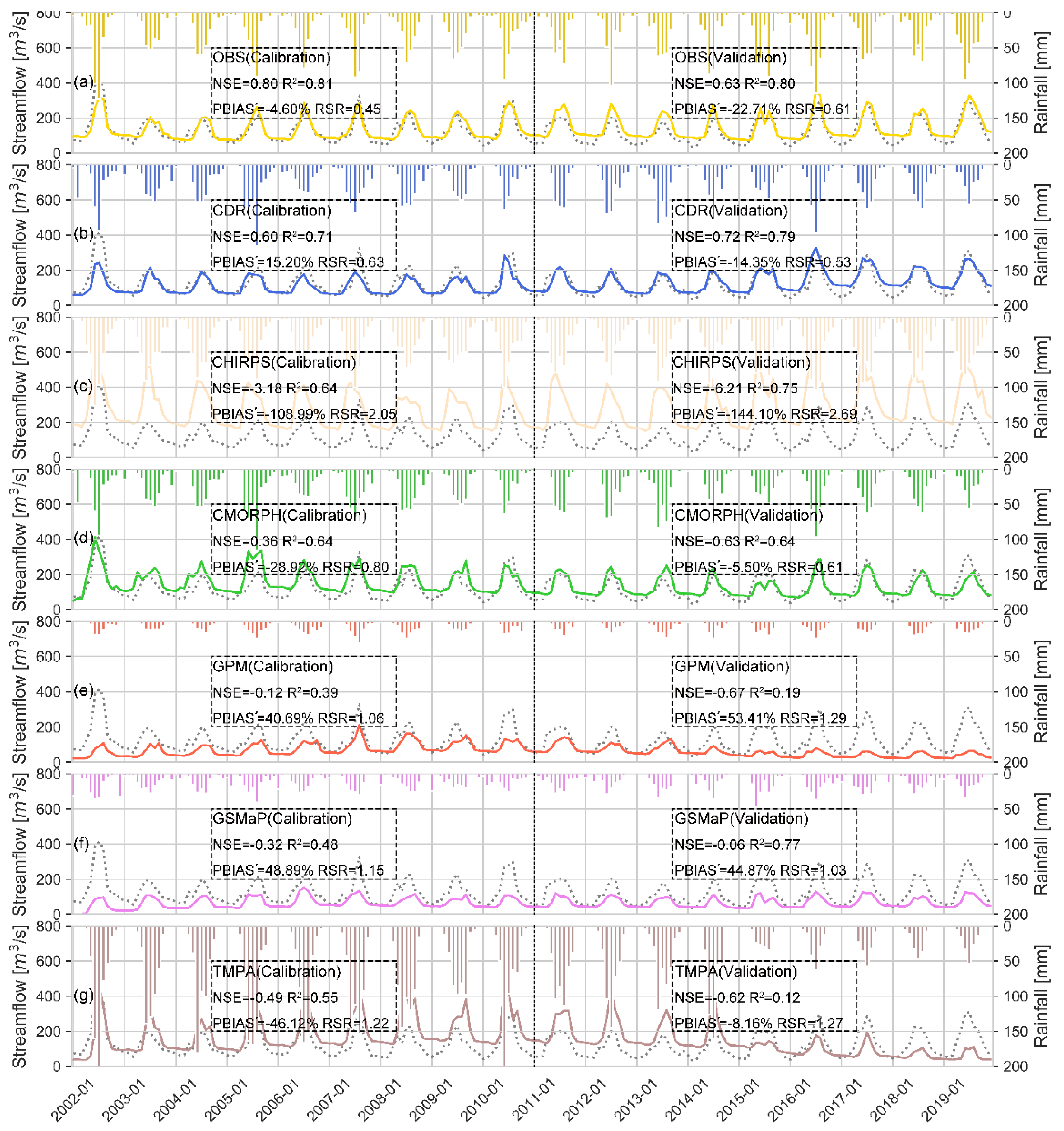
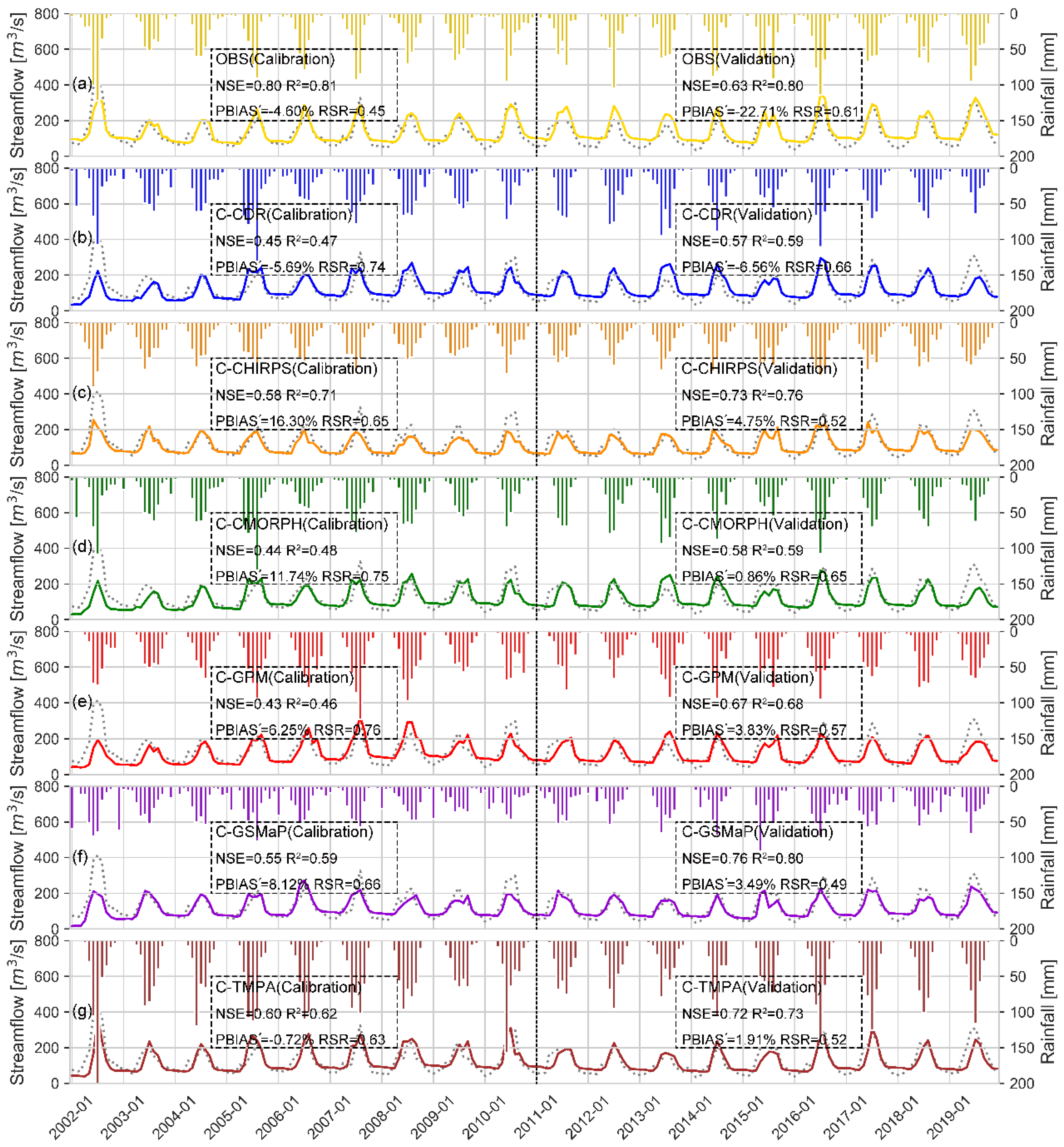
The monthly runoff observation data of the Dashankou hydrological station near the whole watershed outlet was used for calibration. After more than 2000 samplings in a reasonable range of 28 parameters, the model performed well in the calibration period (NSE = 0.80, R2 = 0.81, PBIAS′ = −4.60%, RSR = 0.45). All the indexes declined in the validation period, but they were still satisfactory on the whole (NSE = 0.63, R2 = 0.80, PBIAS′ =−22.71%, RSR = 0.61). With all parameters unchanged, the satellite datasets were input into the SWAT model, and the simulation results are shown in one figure together with the average monthly precipitation. In Figure 10, the bars with different colors represent the monthly average precipitation of each dataset in the whole basin, the grey dotted line represents the monthly observed streamflow, and the solid line with different colors represents the simulated monthly average streamflow of different datasets.
As shown in Figure 10b,d the CDR and CMORPH raw dataset were the two best datasets in the un-corrected streamflow simulation. Among them, the CMORPH overestimated the runoff in the calibration period by −28.92%, which resulted in unsatisfactory simulation results, and the performances of the CDR in the calibration period and the CMORPH in the validation period were all satisfactory. In particular, the performance of the CDR even exceeded the observed data in the validation period with good performance (NSE = 0.72, R2 = 0.79, PBIAS′ = −14.35%, RSR = 0.53).
As the only dataset which overestimated the precipitation in the upper reaches in the spatial distribution evaluation (Figure 6 CHIRPS), the overestimation of CHIRPS in the runoff simulation was also the most obvious in the hydrological simulation, with an overall PBIAS′ of −125.98% (Figure 10c). The vast deviation makes the CHIRPS dataset perform the worst in all indexes except R2 (calibration: NSE = −3.18, PBIAS′ = −108.99%, RSR = 2.05, validation: NSE = −6.21, PBIAS′ = −144.10%, RSR = 2.69.), far away from being satisfactory. On the contrary, the obvious streamflow overestimation of TMPA (Figure 10g, overall PBAIS′: −27.76%) was not reflected in the spatial distribution (Figure 6 TMPA), and this was caused by the temporal variation in the TMPA dataset (Figure 8b). Similarly, the deviation makes the TMPA dataset perform the second worst in the calibration period (NSE = −0.49, PBIAS′ = −46.12%, RSR = 1.22), although the low-level precipitation after 2015 compensated for the overestimation (PBIAS′ drop to −8.16%), other indicators still performed poorly in the validation period of TMPA (NSE = -0.62, R2 = 0.12, RSR = 1.27), and the overall performance was unsatisfactory.
On the contrary, the poor performance of the GPM and GSMaP dataset was mainly due to their underestimation of runoff. As the dataset with the most severe underestimation in the upstream, the underestimation of the GPM dataset was still severe in the runoff simulation, and its total percent bias in all simulation years reached 46.84%. Besides this, all other indexes were unsatisfactory (calibration: NSE = −0.12, RSR = 1.06, validation: NSE = −0.67, RSR = 1.29). Other than that, the linear fitting degree between the simulation results of GPM and the observed runoff was the lowest in all datasets (calibration: R2 = 0.39, validation: R2 = 0.19). The annual average precipitation of the GSMaP was more than that of the GPM (137 mm compared to 118 mm), but the low concentration of precipitation led to high evaporation, which sets the GSMaP at the same underestimation level as the GPM dataset (overall PBIAS′: 47.46%), and the model’s simulation results were also unsatisfactory (calibration: NSE= −0.32, RSR = 1.15, validation: NSE = −0.06, RSR = 1.03). However, the GSMaP dataset showed an excellent linear fit in the whole simulation process, especially in the validation period (R2 = 0.77, ranking second only to the CDR).

3.3.2. Streamflow Simulation of Corrected Satellite Datasets

To increase the applicability of the satellite datasets, a relatively straightforward method was proposed to correct all datasets. To adapt to the calibrated parameters of the SWAT model, the correction was based on the NW station data, and the correction process of each dataset was the same to ensure the comparability between corrected datasets. In particular, the correction processes of the TMPA were divided into two periods due to its apparent differentiation before and after 2015 (Figure 8b, Figure 10g). The corrected datasets were directly inputted into the calibrated SWAT model, and the simulation performance of each dataset was significantly improved except CDR and CMORPH (Table 3). The hydrological simulation results and the corrected monthly precipitation of each dataset were presented in Figure 11.
The processes of dataset correction in this study were intended to enlarge or reduce the original data directly. Therefore, the dataset with a large bias could be improved after correction, while the dataset with small bias may not be promoted obviously (Figure 11b,d). The deviation in the raw CDR dataset was the smallest of all in the hydrological simulation (about 15%), and after correction, the deviation was further reduced (calibration: PBIAS′= −5.69%, validation: PBIAS′= −6.65%). However, other model evaluation indexes were negatively affected (calibration: NSE = 0.45, RSR = 0.74, R2 = 0.47, validation: NSE = 0.57, RSR = 0.66, R2 = 0.59). The overall simulation percent bias of the CMORPH raw dataset was the second smallest (Figure 10d, PBIAS′ = −17.59%). After correction, the simulation result was slightly improved during the calibration period, and slightly decreased during the validation period (Figure 11d), and the overall performance remained unchanged (Table 3).
The two overestimated datasets were significantly improved (Figure 11c,g), and both of them performed “satisfactory” in the calibration period and “good” in the validation period (Table 3). Among them, the improvement of CHIRPS was the largest in all datasets (Overall index, NSE: −4.58 to 0.65, PBIAS′: −125.98% to 10.71%, RSR: 2.36 to 0.59, R2: 0.67 to 0.72). The TMPA dataset was also improved by the correction, especially in the validation period, and the correction exactly filled in the data dislocation before and after 2015, and it is worth noting that the percent bias of TMPA was the smallest of all the datasets (−0.72% in calibration and 1.91% in validation).
The two underestimated datasets also performed better than before (Figure 11e,f). The improvement in the GPM dataset was mainly reflected in the validation period (NSE: 0.67, R2: 0.68, PBIAS′: 3.83%, RSR: 0.57), and although the simulation result was improved to some extent in the calibration period, it was not accurate enough to be evaluated as satisfactory (NSE: 0.43, R2: 0.46, PBIAS′: 6.25%, RSR: 0.76). The GSMaP become the best-performing dataset of all after correction, ranking first in two indexes throughout the whole period (NSE: 0.66, RSR: 0.59). Moreover, the comprehensive evaluation of the GSMaP-driven model reached “very good” in the validation period (NSE: 0.76, R2: 0.80, PBIAS′: 3.49%, RSR: 0.49), which had never occurred in any period of other satellite datasets (Table 3).

4. Discussion

4.1. Outstanding Characteristics of Each Satellite Dataset

The performances of the datasets can vary in different time scales (Table 2), and the CC and precipitation detection indexes, such as POD, FAR, and CSI, were significantly improved with the time scale expansion. Among them, the CDR and CHIRPS had the largest improvement, which was one of their many similar characteristics, such as their excellent performance in winter and stable multi-year mean error. These similarities have also appeared in other studies, possibly because both of them were mainly based on infrared satellite data [6,32]. On a daily scale, GPM was the best dataset in terms of CC in this study, while the best dataset became CDR on the monthly scale. Similar results had also been found in other studies, and the GPM datasets, especially the GPM IMERG final version, performed better on a daily scale than other datasets, but the CDR was more relevant to the observed data on the monthly or annual scale [25,51]. The error-related indexes, such as ME and RMSE, were amplified with the expansion of time scale. Still, there was little change in their deviation degree from the observed data (PBIAS), and some datasets remained almost unchanged (TMPA) or even smaller (GPM). Many studies had shown that TMPA and GPM performed well in bias control when the time scale was extended [9,51,52].
Contrary to the excellent winter performance of CDR and CHIRPS, mentioned above, the CMORPH and TMPA performed poorly in winter (Figure 9), which was mainly due to the limitation of the passive microwave window channels [6,53]. In addition to seasonal differences, the performances of different datasets also vary significantly depending on altitudes. The CDR and GPM datasets show their stability at different altitudes (Figure 5 GPM and Figure 6 CDR), which was critical for the application of satellite datasets at a watershed scale, for the reason that a complete watershed often has a large vertical drop. The underestimation of the GPM in Central Asia was reported in its early evaluation [54], and the dataset was improved in the plain area since the IMERG initial version was developed into the current IMERG Final v06, but its underestimation was still present in the mountain area of the Tianshan Mountain [55]. Conversely, the overestimation of the CMORPH mainly occurred in the plain area of the basin. The overestimation of the CMORPH was common in arid regions; for example, it overestimated the rainfall by an average RMSE of 3.76 mm/d in the Arabian Peninsula, while in Algeria it was 2.32 mm/d [56,57].

4.2. Similarity of the Satellite Datasets

The indexes of each dataset show noticeable zonal distribution on a basin scale, i.e., the wetter the zone was, the more likely it was that the satellite datasets tended to underestimate, had a better fit degree, and hit more rainfall events (Figure 4a,d,g). A similar performance had also been found in Indochina Peninsula and Pakistan [25,27,58]. Comparatively speaking, the influence of terrain factors was weaker; for instance, the fitting degrees and the underestimation of the datasets in the low-altitude wet mountain area were stronger than those in the high-altitude dry mountain area of the Hanjiang River Basin [24]. On a global scale, it was clear that all datasets performed better in the low-latitude regions, such as the Philippines and Ethiopia, or coastal areas of mid-latitudes, such as Northeast China [9,43,51]. As a part of the arid land in Central Asia, this study area was one of the worst-performing regions for satellite datasets, which was also supported by some global or large regional studies [5,6].
All datasets performed poorly in winter, with the CC range from 0 to 0.15 and the CSI range from 0 to 0.10. Even for those based on infrared remote sensing, winter was still their worst-performing season of the year (Figure 7a,c and Figure 9.). The inaccurate estimation of the datasets in winter was one of the reasons for their poor performance in the temperate zone, which was also a challenge for the current satellite precipitation retrievals [59]. Each dataset showed varying degrees of improvement in the multi-year performance evaluation (Figure 8a), and some studies believe that the improvement of precipitation datasets in the multi-year performance evaluation was due to technological progress [60]. Nevertheless, the slight dataset improvement in this study cannot be simply summed up by technological progress. For the passive microwave products, the reason might be the increase in passive microwave samples [6]. For datasets that do not rely on the passive microwave, such as CDR and CHIRPS, their improvement was more likely to be caused by the slight increase in precipitation under climate change [61].

4.3. Similarities and Differences in the Datasets Hydrological Application

The raw data of CDR showed a strong ability in the monthly runoff simulation (Figure 10a), which was consistent with its excellent performance in monthly rainfall and winter precipitation estimations (Table 2 and Figure 9). Furthermore, the advantage of the CDR in the monthly runoff simulation was mainly manifested in relatively high latitude areas, such as the Illinois River Basin [62], but was not prominent in low latitude areas [9,25]. The dislocation of TMPA data around 2015 (Figure 10g) was likely to be affected by its new generation product GPM, and 2015 is the first year after the release of the GPM [19]. In the same study area, TMPA performed much better when the evaluation period changed to 2000–2015 [63]. Compared with the complex and targeted correction methods for each dataset, the method used in this study is simple and direct, so as to avoid introducing other interference factors that may affect the comparison between datasets.
The performance of the corrected dataset in the validation period was better than that in the calibration period (Figure 11), which was consistent with the dataset’s performance in the multi-year evaluation (Figure 8a), and besides this, more warm-up years would lead to better simulation results in the hydrological model [64], which was another reason for the excellent performance in the validation period. Some studies suggest that the observed stations play an irreplaceable role in the watershed-scale hydrological simulation [26,42]. On the other hand, integrating the performance of the uncorrected and corrected satellite datasets into hydrological simulation, all datasets were “satisfactory” or better in this study (Table 3), which means that the satellite precipitation datasets could be a favorable choice for data-scarce basins [7,9,65].

4.4. Further Study

For some of the content, the distribution of observed stations may affect their comparison with satellite precipitation datasets, which was also a common issue in the research of datasets evaluation and hydrological modeling [7]. The meteorological stations tend to be dense in plain areas and sparse in high-altitude mountainous areas. In this study, there is only one station available for the hydrological modeling within the upstream basin boundary, which may lead to the underestimation of the precipitation input compared with the actual value [66]. Consequently, the evenly distributed RG station could be used for dataset correction and hydrological modeling in the follow-up study; thus the processing of the winter input data will be a challenge, and a discussion of the rationality of the model’s parameters is necessary.

5. Conclusions

This study evaluated the performances of six gauge-adjusted version satellite precipitation datasets, including PERSIANN-CDR_V1_R1, CHIRPS_2.0, CMORPH_IFlOODS_V1.0, GPM_IMERGF_V06, GSMaP_V6, and TMPA_3B42_daily_V7 at a watershed scale, regarding a typical arid land watershed of Central Asia. The research work mainly includes the evaluation of the datasets’ accuracy and the hydrological model’s applicability, and the findings of this research can be summarized as follows:
  • The GPM was the best dataset in the daily scale rainfall evaluation. It had the best correlation with observed data, minimum RMSE, slight underestimation, and a reasonably good rainfall detection ability. The CHIRPS and CMORPH performed relatively poorly on a daily scale. Among them, CHIRPS had the worst rainfall detection skill, while CMORPH excessively overestimated the rainfall;
  • The CDR was the best dataset in the monthly scale rainfall evaluation, with excellent agreement with observed data (ranked first in CC, RMSE, ME, and PBIAS) and a pretty good rainfall detection ability. In contrast, the CMORPH performed deficiently due to its remaining overestimation. Meanwhile, the TMPA had many unsatisfying indexes (rank 6th in CC, rank 5th in RMSE and PBIAS) and performed ineffectively in monthly rainfall estimation compared to others;
  • In wetter regions of the basin, all six datasets tended to perform better. The spatial distribution of CDR and GPM was the most uniform, among which the CDR had the smallest error value and error differentiation in different locations of the basin, and the GPM performed well in correlation with gauge stations in the whole basin;
  • In the multi-year evaluation, the correlation between each dataset and the NW stations was improving with time, especially during the rainy season (from April to October); among them, the GPM had the largest increase. For the evaluation within the year, the CDR and CHIRPS were the two best datasets in the winter performance, and all datasets tended to perform better in the summer;
  • In the application of the hydrological model, the CDR-driven model had the most outstanding performance out of the raw satellite datasets, and was even better than the observed data-driven model in some years. In the rest of the other datasets, the CHIRPS and TMPA overestimated the streamflow in their driven models. At the same time, the GPM and GSMaP underestimated the streamflow in their driven models, and the CMORPH was the only dataset that was close to being qualified as “satisfactory”.
  • After a simple correction, those datasets with large deviations could get good results in terms of hydrological modeling. Taking everything into account, satellite precipitation datasets can serve as an alternative for the related hydrological research in data-scarce areas.

Supplementary Materials

The following are available online at https://www.mdpi.com/2072-4292/13/2/221/s1, Table S1: SWAT model sensitive parameters of the Kaidu River Upper Basin.

Author Contributions

Framework design, T.L., Y.H. and P.D.M.; methodology, J.P., T.L. and Y.L.; software, Z.L.; validation, J.P. and Y.L.; formal analysis, J.P.; investigation, J.P.; data curation, Z.L.; writing—original draft preparation, J.P.; writing—review and editing, T.L. and Y.H.; visualization, J.P. and Y.L.; supervision, A.K. and P.D.M.; project administration, A.B. and X.C.; funding acquisition, A.B. and X.C. All authors have read and agreed to the published version of the manuscript.

Funding

This study was supported by the National Key Research and Development Plan of China (Grant No.2017YFB0504204), Strategic Priority Research Program of the Chinese Academy of Sciences, Pan-Third Pole Environment Study for a Green Silk Road (Grant No. XDA20060303), the State’s Key Project of Research and Development Plan (Grant No. 2017YFC0404501), the National Natural Science Foundation of China (Grant No. 41761144079), the International Partnership Program of the Chinese Academy of Sciences (Grant No. 131551KYS B20160002), CAS Interdisplinary Innovation Team (Grant No. JCTD-2019-20), CAS Research Center for Ecology and Environment of Central Asia (Grant No. Y934031) and Regional Collaborative Innovation Project of Xinjiang Uygur Autonomous Regions (Grant No. 2020E01010).

Institutional Review Board Statement

Not applicable.

Informed Consent Statement

Not applicable.

Data Availability Statement

Data sharing not applicable.

Acknowledgments

We acknowledge the Xinjiang Meteorological Service and the National Meteorology Information Centre for sharing meteorological data. A special acknowledgement should be expressed to China–Pakistan Joint Research Center on Earth Sciences that supported the implementation of this study.

Conflicts of Interest

The authors declare no conflict of interest.

References

  1. Faurès, J.-M.; Goodrich, D.C.; Woolhiser, D.A.; Sorooshian, S. Impact of small-scale spatial rainfall variability on runoff modeling. J. Hydrol. 1995, 173, 309–326. [Google Scholar] [CrossRef]
  2. Faridzad, M.; Yang, T.; Hsu, K.; Sorooshian, S.; Xiao, C. Rainfall frequency analysis for ungauged regions using remotely sensed precipitation information. J. Hydrol. 2018, 563, 123–142. [Google Scholar] [CrossRef] [Green Version]
  3. Ebert, E.E.; Janowiak, J.E.; Kidd, C. Comparison of Near-Real-Time Precipitation Estimates from Satellite Observations and Numerical Models. Bull. Am. Meteorol. Soc. 2007, 88, 47–64. [Google Scholar] [CrossRef] [Green Version]
  4. Bharti, V.; Singh, C. Evaluation of error in TRMM 3B42V7 precipitation estimates over the Himalayan region. J. Geophys. Res. Atmos. 2015, 120, 12458–12473. [Google Scholar] [CrossRef]
  5. Beck, H.E.; Vergopolan, N.; Pan, M.; Levizzani, V.; van Dijk, A.I.J.M.; Weedon, G.P.; Brocca, L.; Pappenberger, F.; Huffman, G.J.; Wood, E.F. Global-scale evaluation of 22 precipitation datasets using gauge observations and hydrological modeling. Hydrol. Earth Syst. Sci. 2017, 21, 6201–6217. [Google Scholar] [CrossRef] [Green Version]
  6. Tang, G.; Clark, M.P.; Papalexiou, S.M.; Ma, Z.; Hong, Y. Have satellite precipitation products improved over last two decades? A comprehensive comparison of GPM IMERG with nine satellite and reanalysis datasets. Remote Sens. Environ. 2020, 240, 111697. [Google Scholar] [CrossRef]
  7. Tuo, Y.; Duan, Z.; Disse, M.; Chiogna, G. Evaluation of precipitation input for SWAT modeling in Alpine catchment: A case study in the Adige river basin (Italy). Sci. Total Environ. 2016, 573, 66–82. [Google Scholar] [CrossRef] [Green Version]
  8. Chen, C.-J.; Senarath, S.U.S.; Dima-West, I.M.; Marcella, M.P. Evaluation and restructuring of gridded precipitation data over the Greater Mekong Subregion. Int. J. Climatol. 2017, 37, 180–196. [Google Scholar] [CrossRef]
  9. Musie, M.; Sen, S.; Srivastava, P. Comparison and evaluation of gridded precipitation datasets for streamflow simulation in data scarce watersheds of Ethiopia. J. Hydrol. 2019, 579, 124168. [Google Scholar] [CrossRef]
  10. Essou, G.R.C.; Arsenault, R.; Brissette, F.P. Comparison of climate datasets for lumped hydrological modeling over the continental United States. J. Hydrol. 2016, 537, 334–345. [Google Scholar] [CrossRef]
  11. Ur Rahman, K.; Shang, S.; Shahid, M.; Wen, Y. Hydrological evaluation of merged satellite precipitation datasets for streamflow simulation using SWAT: A case study of Potohar Plateau, Pakistan. J. Hydrol. 2020, 587, 125040. [Google Scholar] [CrossRef]
  12. Ben Aissia, M.-A.; Chebana, F.; Ouarda, T.B.M.J. Multivariate missing data in hydrology—Review and applications. Adv. Water Resour. 2017, 110, 299–309. [Google Scholar] [CrossRef] [Green Version]
  13. Taylor, C.M.; Belušić, D.; Guichard, F.; Parker, D.J.; Vischel, T.; Bock, O.; Harris, P.P.; Janicot, S.; Klein, C.; Panthou, G. Frequency of extreme Sahelian storms tripled since 1982 in satellite observations. Nature 2017, 544, 475–478. [Google Scholar] [CrossRef] [PubMed] [Green Version]
  14. Mölg, T.; Maussion, F.; Scherer, D. Mid-latitude westerlies as a driver of glacier variability in monsoonal High Asia. Nat. Clim. Chang. 2014, 4, 68–73. [Google Scholar] [CrossRef]
  15. Sun, Q.; Miao, C.; Duan, Q.; Ashouri, H.; Sorooshian, S.; Hsu, K.-L. A Review of Global Precipitation Data Sets: Data Sources, Estimation, and Intercomparisons. Rev. Geophys. 2018, 56, 79–107. [Google Scholar] [CrossRef] [Green Version]
  16. Kummerow, C.; Barnes, W.; Kozu, T.; Shiue, J.; Simpson, J. The Tropical Rainfall Measuring Mission (TRMM) Sensor Package. J. Atmos. Ocean. Technol. 1998, 15, 809–817. [Google Scholar] [CrossRef]
  17. Kidd, C.; Huffman, G. Global precipitation measurement. Meteorol. Appl. 2011, 18, 334–353. [Google Scholar] [CrossRef]
  18. Huffman, G.J.; Bolvin, D.T.; Nelkin, E.J.; Wolff, D.B.; Adler, R.F.; Gu, G.; Hong, Y.; Bowman, K.P.; Stocker, E.F. The TRMM Multisatellite Precipitation Analysis (TMPA): Quasi-Global, Multiyear, Combined-Sensor Precipitation Estimates at Fine Scales. J. Hydrometeorol. 2007, 8, 38–55. [Google Scholar] [CrossRef]
  19. Hou, A.Y.; Kakar, R.K.; Neeck, S.; Azarbarzin, A.A.; Kummerow, C.D.; Kojima, M.; Oki, R.; Nakamura, K.; Iguchi, T. The Global Precipitation Measurement Mission. Bull. Am. Meteorol. Soc. 2014, 95, 701–722. [Google Scholar] [CrossRef]
  20. Sorooshian, S.; Hsu, K.-L.; Gao, X.; Gupta, H.V.; Imam, B.; Braithwaite, D. Evaluation of PERSIANN System Satellite-Based Estimates of Tropical Rainfall. Bull. Am. Meteorol. Soc. 2000, 81, 2035–2046. [Google Scholar] [CrossRef] [Green Version]
  21. Funk, C.C.; Peterson, P.J.; Landsfeld, M.F.; Pedreros, D.H.; Verdin, J.P.; Rowland, J.D.; Romero, B.E.; Husak, G.J.; Michaelsen, J.C.; Verdin, A.P. A Quasi-Global Precipitation Time Series for Drought Monitoring; Data Series 832; U.S. Geological Survey: Reston, VA, USA, 2014; p. 12. [Google Scholar]
  22. Kubota, T.; Shige, S.; Hashizume, H.; Aonashi, K.; Takahashi, N.; Seto, S.; Hirose, M.; Takayabu, Y.N.; Ushio, T.; Nakagawa, K.; et al. Global Precipitation Map Using Satellite-Borne Microwave Radiometers by the GSMaP Project: Production and Validation. IEEE Trans. Geosci. Remote Sens. 2007, 45, 2259–2275. [Google Scholar] [CrossRef]
  23. Joyce, R.J.; Janowiak, J.E.; Arkin, P.A.; Xie, P. CMORPH: A Method that Produces Global Precipitation Estimates from Passive Microwave and Infrared Data at High Spatial and Temporal Resolution. J. Hydrometeorol. 2004, 5, 487–503. [Google Scholar] [CrossRef]
  24. Deng, P.; Zhang, M.; Bing, J.; Jia, J.; Zhang, D. Evaluation of the GSMaP_Gauge products using rain gauge observations and SWAT model in the Upper Hanjiang River Basin. Atmos. Res. 2019, 219, 153–165. [Google Scholar] [CrossRef]
  25. Le, M.-H.; Lakshmi, V.; Bolten, J.; Bui, D.D. Adequacy of Satellite-derived Precipitation Estimate for Hydrological Modeling in Vietnam Basins. J. Hydrol. 2020, 586, 124820. [Google Scholar] [CrossRef]
  26. Chen, J.; Li, Z.; Li, L.; Wang, J.; Qi, W.; Xu, C.-Y.; Kim, J.-S. Evaluation of Multi-Satellite Precipitation Datasets and Their Error Propagation in Hydrological Modeling in a Monsoon-Prone Region. Remote Sens. 2020, 12, 3550. [Google Scholar] [CrossRef]
  27. Tang, X.; Zhang, J.; Gao, C.; Ruben, B.G.; Wang, G. Assessing the Uncertainties of Four Precipitation Products for Swat Modeling in Mekong River Basin. Remote Sens. 2019, 11, 304. [Google Scholar] [CrossRef] [Green Version]
  28. Massari, C.; Brocca, L.; Pellarin, T.; Abramowitz, G.; Filippucci, P.; Ciabatta, L.; Maggioni, V.; Kerr, Y.; Fernandez Prieto, D. A daily 25 km short-latency rainfall product for data-scarce regions based on the integration of the Global Precipitation Measurement mission rainfall and multiple-satellite soil moisture products. Hydrol. Earth Syst. Sci. 2020, 24, 2687–2710. [Google Scholar] [CrossRef]
  29. Liu, T.; Willems, P.; Pan, X.L.; Bao, A.M.; Chen, X.; Veroustraete, F.; Dong, Q.H. Climate change impact on water resource extremes in a headwater region of the Tarim basin in China. Hydrol. Earth Syst. Sci. 2011, 15, 3511–3527. [Google Scholar] [CrossRef] [Green Version]
  30. Ma, Y.; Huang, Y.; Liu, T. Change and Climatic Linkage for Extreme Flows in Typical Catchments of Middle Tianshan Mountain, Northwest China. Water 2018, 10, 1061. [Google Scholar] [CrossRef] [Green Version]
  31. Guo, H.; Bao, A.; Ndayisaba, F.; Liu, T.; Kurban, A.; De Maeyer, P. Systematical Evaluation of Satellite Precipitation Estimates Over Central Asia Using an Improved Error-Component Procedure. J. Geophys. Res. Atmos. 2017, 122, 10906–10927. [Google Scholar] [CrossRef]
  32. Gao, F.; Zhang, Y.; Chen, Q.; Wang, P.; Yang, H.; Yao, Y.; Cai, W. Comparison of two long-term and high-resolution satellite precipitation datasets in Xinjiang, China. Atmos. Res. 2018, 212, 150–157. [Google Scholar] [CrossRef]
  33. Pereira-Cardenal, S.J.; Riegels, N.D.; Berry, P.A.M.; Smith, R.G.; Yakovlev, A.; Siegfried, T.U.; Bauer-Gottwein, P. Real-time remote sensing driven river basin modeling using radar altimetry. Hydrol. Earth Syst. Sci. 2011, 15, 241–254. [Google Scholar] [CrossRef]
  34. Luo, M.; Liu, T.; Meng, F.; Duan, Y.; Frankl, A.; Bao, A.; De Maeyer, P. Comparing Bias Correction Methods Used in Downscaling Precipitation and Temperature from Regional Climate Models: A Case Study from the Kaidu River Basin in Western China. Water 2018, 10, 1046. [Google Scholar] [CrossRef] [Green Version]
  35. Ashouri, H.; Hsu, K.-L.; Sorooshian, S.; Braithwaite, D.K.; Knapp, K.R.; Cecil, L.D.; Nelson, B.R.; Prat, O.P. PERSIANN-CDR: Daily Precipitation Climate Data Record from Multisatellite Observations for Hydrological and Climate Studies. Bull. Am. Meteorol. Soc. 2015, 96, 69–83. [Google Scholar] [CrossRef] [Green Version]
  36. Funk, C.; Peterson, P.; Landsfeld, M.; Pedreros, D.; Verdin, J.; Shukla, S.; Husak, G.; Rowland, J.; Harrison, L.; Hoell, A.; et al. The climate hazards infrared precipitation with stations—A new environmental record for monitoring extremes. Sci. Data 2015, 2, 150066. [Google Scholar] [CrossRef] [Green Version]
  37. Xie, P.; Joyce, R.; Wu, S.; Yoo, S.-H.; Yarosh, Y.; Sun, F.; Lin, R. Reprocessed, Bias-Corrected CMORPH Global High-Resolution Precipitation Estimates from 1998. J. Hydrometeorol. 2017, 18, 1617–1641. [Google Scholar] [CrossRef]
  38. Huffman, G.J.; Stocker, E.F.; Bolvin, D.T.; Nelkin, E.J.; Tan, J. GPM IMERG Final Precipitation L3 1 Day 0.1 Degree x 0.1 Degree V06. DISC); Technical Report No.; Savtchenko, A., Ed.; Goddard Earth Sciences Data and Information Services Center (GES DISC): Greenbelt, MD, USA, 2019. [Google Scholar] [CrossRef]
  39. Kubota, T.; Aonashi, K.; Ushio, T.; Shige, S.; Takayabu, Y.N.; Kachi, M.; Arai, Y.; Tashima, T.; Masaki, T.; Kawamoto, N.; et al. Global Satellite Mapping of Precipitation (GSMaP) Products in the GPM Era. In Satellite Precipitation Measurement: Volume 1; Levizzani, V., Kidd, C., Kirschbaum, D.B., Kummerow, C.D., Nakamura, K., Turk, F.J., Eds.; Springer International Publishing: Cham, Switzerland, 2020; pp. 355–373. [Google Scholar] [CrossRef]
  40. Huffman, G.J.; Bolvin, D.T.; Nelkin, E.J.; Adler, R.F. TRMM (TMPA) Precipitation L3 1 Day 0.25 Degree x 0.25 Degree V7. DISC); Technical Report No.; Savtchenko, A., Ed.; Goddard Earth Sciences Data and Information Services Center (GES DISC): Greenbelt, MD, USA, 2016. [Google Scholar] [CrossRef]
  41. Arnold, J.G.; Moriasi, N.D.; Gassman, W.P.; Abbaspour, C.K.; White, J.M.; Srinivasan, R.; Santhi, C.; Harmel, D.R.; van Griensven, A.; Van Liew, W.M.; et al. SWAT: Model Use, Calibration, and Validation. Trans. ASABE 2012, 55, 1491–1508. [Google Scholar] [CrossRef]
  42. Wang, N.; Liu, W.; Sun, F.; Yao, Z.; Wang, H.; Liu, W. Evaluating satellite-based and reanalysis precipitation datasets with gauge-observed data and hydrological modeling in the Xihe River Basin, China. Atmos. Res. 2020, 234, 104746. [Google Scholar] [CrossRef]
  43. Zhu, H.; Li, Y.; Huang, Y.; Li, Y.; Hou, C.; Shi, X. Evaluation and hydrological application of satellite-based precipitation datasets in driving hydrological models over the Huifa river basin in Northeast China. Atmos. Res. 2018, 207, 28–41. [Google Scholar] [CrossRef]
  44. Moriasi, N.D.; Arnold, G.J.; Van Liew, W.M.; Bingner, L.R.; Harmel, D.R.; Veith, L.T. Model Evaluation Guidelines for Systematic Quantification of Accuracy in Watershed Simulations. Trans. ASABE 2007, 50, 885–900. [Google Scholar] [CrossRef]
  45. Briggs, W. Statistical Methods in the Atmospheric Sciences. J. Am. Stat. Assoc. 2007, 102, 380. [Google Scholar] [CrossRef]
  46. Nash, J.E.; Sutcliffe, J.V. River flow forecasting through conceptual models part I—A discussion of principles. J. Hydrol. 1970, 10, 282–290. [Google Scholar] [CrossRef]
  47. Tao, Y.; Gao, X.; Hsu, K.; Sorooshian, S.; Ihler, A. A Deep Neural Network Modeling Framework to Reduce Bias in Satellite Precipitation Products. J. Hydrometeorol. 2016, 17, 931–945. [Google Scholar] [CrossRef]
  48. Yin, Z.-Y.; Liu, X.; Zhang, X.; Chung, C.-F. Using a geographic information system to improve Special Sensor Microwave Imager precipitation estimates over the Tibetan Plateau. J. Geophys. Res. Atmos. 2004, 109. [Google Scholar] [CrossRef]
  49. Greene, J.S.; Morrissey, M.L. Validation and Uncertainty Analysis of Satellite Rainfall Algorithms. Prof. Geogr. 2000, 52, 247–258. [Google Scholar] [CrossRef]
  50. Habib, E.; Haile, A.T.; Sazib, N.; Zhang, Y.; Rientjes, T. Effect of Bias Correction of Satellite-Rainfall Estimates on Runoff Simulations at the Source of the Upper Blue Nile. Remote Sens. 2014, 6, 6688–6708. [Google Scholar] [CrossRef] [Green Version]
  51. Tan, M.L.; Santo, H. Comparison of GPM IMERG, TMPA 3B42 and PERSIANN-CDR satellite precipitation products over Malaysia. Atmos. Res. 2018, 202, 63–76. [Google Scholar] [CrossRef]
  52. Ullah, W.; Wang, G.; Ali, G.; Tawia Hagan, D.F.; Bhatti, A.S.; Lou, D. Comparing Multiple Precipitation Products against In-Situ Observations over Different Climate Regions of Pakistan. Remote Sens. 2019, 11, 628. [Google Scholar] [CrossRef] [Green Version]
  53. Yong, B.; Hong, Y.; Ren, L.-L.; Gourley, J.J.; Huffman, G.J.; Chen, X.; Wang, W.; Khan, S.I. Assessment of evolving TRMM-based multisatellite real-time precipitation estimation methods and their impacts on hydrologic prediction in a high latitude basin. J. Geophys. Res. Atmos. 2012, 117. [Google Scholar] [CrossRef] [Green Version]
  54. Guo, H.; Chen, S.; Bao, A.; Behrangi, A.; Hong, Y.; Ndayisaba, F.; Hu, J.; Stepanian, P.M. Early assessment of Integrated Multi-satellite Retrievals for Global Precipitation Measurement over China. Atmos. Res. 2016, 176–177, 121–133. [Google Scholar] [CrossRef]
  55. Zhou, Z.; Guo, B.; Xing, W.; Zhou, J.; Xu, F.; Xu, Y. Comprehensive evaluation of latest GPM era IMERG and GSMaP precipitation products over mainland China. Atmos. Res. 2020, 246, 105132. [Google Scholar] [CrossRef]
  56. Babaousmail, H.; Hou, R.; Ayugi, B.; Gnitou, G.T. Evaluation of satellite-based precipitation estimates over Algeria during 1998–2016. J. Atmos. Sol. Terr. Phys. 2019, 195, 105139. [Google Scholar] [CrossRef]
  57. Alsumaiti, T.S.; Hussein, K.; Ghebreyesus, D.T.; Sharif, H.O. Performance of the CMORPH and GPM IMERG Products over the United Arab Emirates. Remote Sens. 2020, 12, 1426. [Google Scholar] [CrossRef]
  58. Hussain, Y.; Satgé, F.; Hussain, M.B.; Martinez-Carvajal, H.; Bonnet, M.-P.; Cárdenas-Soto, M.; Roig, H.L.; Akhter, G. Performance of CMORPH, TMPA, and PERSIANN rainfall datasets over plain, mountainous, and glacial regions of Pakistan. Theor. Appl. Climatol. 2018, 131, 1119–1132. [Google Scholar] [CrossRef]
  59. Yong, B.; Chen, B.; Gourley, J.J.; Ren, L.; Hong, Y.; Chen, X.; Wang, W.; Chen, S.; Gong, L. Intercomparison of the Version-6 and Version-7 TMPA precipitation products over high and low latitudes basins with independent gauge networks: Is the newer version better in both real-time and post-real-time analysis for water resources and hydrologic extremes? J. Hydrol. 2014, 508, 77–87. [Google Scholar] [CrossRef]
  60. Eini, M.R.; Javadi, S.; Delavar, M.; Monteiro, J.A.F.; Darand, M. High accuracy of precipitation reanalyses resulted in good river discharge simulations in a semi-arid basin. Ecol. Eng. 2019, 131, 107–119. [Google Scholar] [CrossRef]
  61. Yang, H.; Xu, J.; Chen, Y.; Li, D.; Zuo, J.; Zhu, N.; Chen, Z. Has the Bosten Lake Basin been dry or wet during the climate transition in Northwest China in the past 30 years? Theor. Appl. Climatol. 2020, 141, 627–644. [Google Scholar] [CrossRef]
  62. Behrangi, A.; Khakbaz, B.; Jaw, T.C.; AghaKouchak, A.; Hsu, K.; Sorooshian, S. Hydrologic evaluation of satellite precipitation products over a mid-size basin. J. Hydrol. 2011, 397, 225–237. [Google Scholar] [CrossRef] [Green Version]
  63. Chen, C.; Li, Z.; Song, Y.; Duan, Z.; Mo, K.; Wang, Z.; Chen, Q. Performance of Multiple Satellite Precipitation Estimates over a Typical Arid Mountainous Area of China: Spatiotemporal Patterns and Extremes. J. Hydrometeorol. 2020, 21, 533–550. [Google Scholar] [CrossRef]
  64. Kim, K.B.; Kwon, H.-H.; Han, D. Exploration of warm-up period in conceptual hydrological modelling. J. Hydrol. 2018, 556, 194–210. [Google Scholar] [CrossRef] [Green Version]
  65. Khoshchehreh, M.; Ghomeshi, M.; Shahbazi, A. Hydrological evaluation of global gridded precipitation datasets in a heterogeneous and data-scarce basin in Iran. J. Earth Syst. Sci. 2020, 129, 201. [Google Scholar] [CrossRef]
  66. Isotta, F.A.; Frei, C.; Weilguni, V.; Perčec Tadić, M.; Lassègues, P.; Rudolf, B.; Pavan, V.; Cacciamani, C.; Antolini, G.; Ratto, S.M.; et al. The climate of daily precipitation in the Alps: Development and analysis of a high-resolution grid dataset from pan-Alpine rain-gauge data. Int. J. Climatol. 2014, 34, 1657–1675. [Google Scholar] [CrossRef]
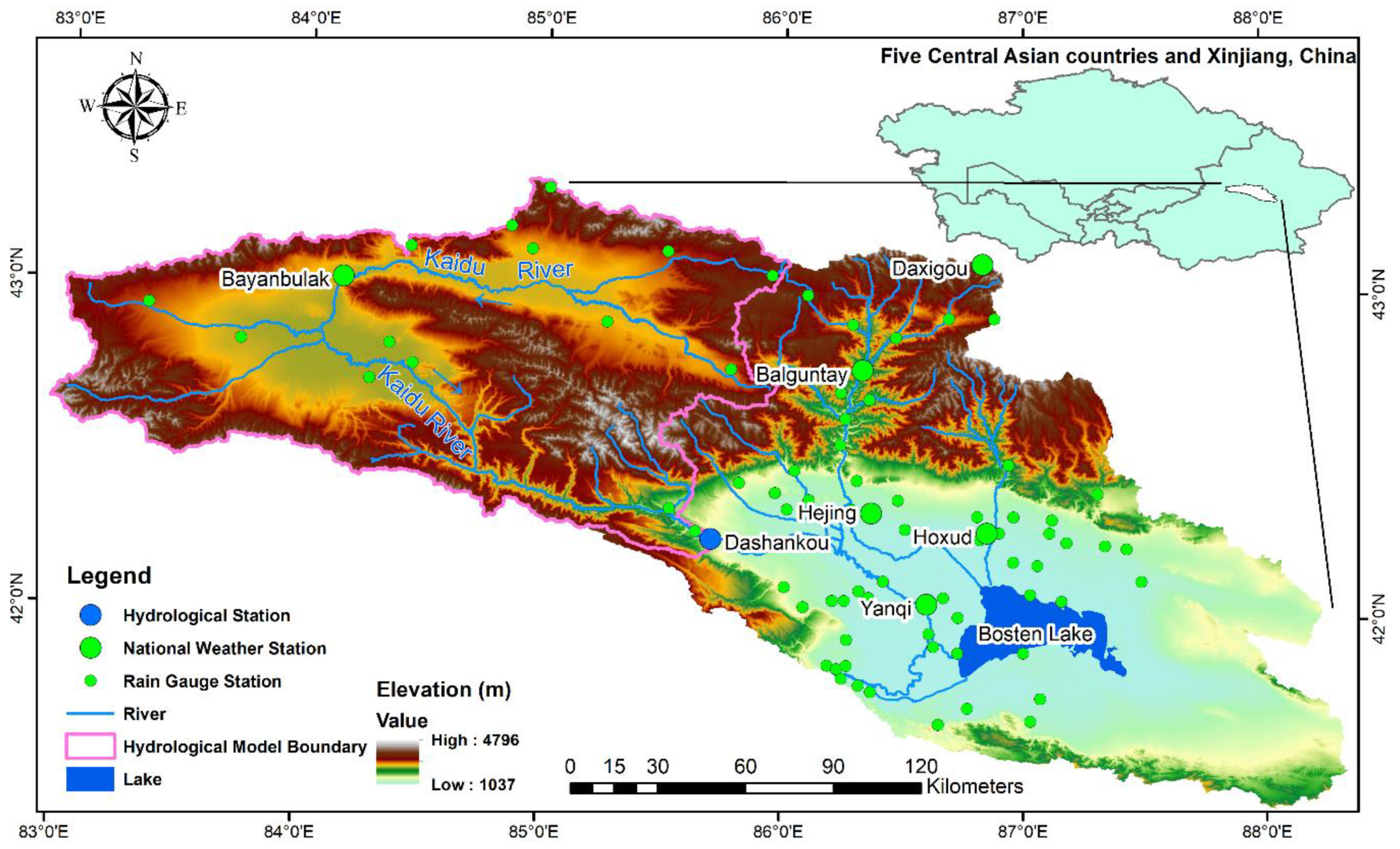
Figure 1. Study area (based on map sources: Department of Natural Resources of Xinjiang Uygur Autonomous Regions Xin S (2019) No.044).
Remotesensing 13 00221 g001
Figure 2. The performance of daily data in different evaluation indexes. (The point represents the outlier. For the whiskers, the upper and lower boundaries represent the maximum value and minimum value, respectively. For the boxes with color, the top, middle and bottom black lines represent first quartile value, median value, and third quartile value, respectively.) (a) Correlation coefficient, (b) root mean square error, (c) mean error, (d) percentage bias, (e) probability of detection, (f) false alarm ratio, (g) critical success index.
Remotesensing 13 00221 g002
Figure 3. The performance of monthly data in different evaluation indexes. (The point represents the outlier. For the whiskers, the upper and lower boundaries represent the maximum value and minimum values, respectively. For the boxes with color, the top, middle and bottom black lines represent first quartile value, median value, and third quartile value, respectively.) (a) Correlation coefficient, (b) root mean square error, (c) mean error, (d) percentage bias, (e) probability of detection, (f) false alarm ratio, (g) critical success index.
Remotesensing 13 00221 g003
Figure 4. Datasets’ daily scale performance under different annual rainfall intensities (mm/a). (a) Correlation coefficient, (b) root mean square error, (c) mean error, (d) percentage bias, (e) probability of detection, (f) false alarm ratio, (g) critical success index.
Remotesensing 13 00221 g004
Figure 5. Distribution of CC between satellite datasets and measured data at different stations in the basin.
Remotesensing 13 00221 g005
Figure 6. Distribution of ME between satellite datasets and measured data at different stations in the basin.
Remotesensing 13 00221 g006
Figure 7. Distribution of the evaluation indexes in every month based on NW station daily data. (a) Correlation coefficient, (b) mean error, (c) critical success index.
Remotesensing 13 00221 g007
Figure 8. Smooth line chart of the distribution of the evaluation indexes in every year from 1998 to 2019 based on NW station daily data. (a) Correlation coefficient, (b) mean error, (c) critical success index.
Remotesensing 13 00221 g008
Figure 9. Annual correlation coefficient changes in different months of each dataset based on NW station daily data. (a) CDR, (b) CHIRPS, (c) CMORPH, (d) GPM, (e) GSMaP, (f) TMPA.
Remotesensing 13 00221 g009
Figure 10. Average monthly precipitation and monthly streamflow simulation results of NW station data and six raw satellite datasets in the calibration period (2002–2010) and the validation period (2011–2019). (a) Observed data, (b) CDR, (c) CHIRPS, (d) CMORPH, (e) GPM, (f) GSMaP, (g) TMPA.
Remotesensing 13 00221 g010
Figure 11. Average monthly precipitation and monthly streamflow simulation results of NW station data and six corrected satellite datasets in the calibration period (2002–2010) and the validation period (2011–2019).(a) Observed data, (b) CDR, (c) CHIRPS, (d) CMORPH, (e) GPM, (f) GSMaP, (g) TMPA.
Remotesensing 13 00221 g011
Table 1. Summary of satellite precipitation datasets used in this study.
Dataset VersionShort NameRelease DateResolutionPeriod
PERSIANN-CDR_V1_R1CDR20140.25°/1 d1983–present
CHIRPS_2.0CHIRPS20150.25°/1 d1981–present
CMORPH_IFlOODS_V1.0CMORPH20130.25°/1 d1998–2019
GPM_IMERGF_V06GPM20190.10°/1 d2000–present
GSMaP_V6GSMaP20160.25°/1 d2000–present
TMPA_3B42_daily_V7TMPA20160.25°/1 d1998–2019
Table 2. Average evaluation indexes of all station points at both the daily and monthly scale.
Time ScaleSatellite DataCCRMSE
(mm)
ME(mm) *PBIAS(%) *PODFARCSI
DailyCDR0.322.380.04 (0.25)29.92 (46.96)0.870.740.25
CHIRPS0.293.030.19 (0.25)40.60 (49.35)0.460.660.24
CMORPH0.433.220.86 (1.08)244.82 (260.23)0.810.700.27
GPM0.522.27−0.38 (0.38)−43.28 (45.08)0.770.610.34
GSMaP0.402.560.11 (0.25)39.87 (49.70)0.870.670.32
TMPA0.312.790.11 (0.47)56.31 (93.87)0.590.530.34
MonthlyCDR0.6917.811.15 (7.69)30.98 (48.15)1.000.160.84
CHIRPS0.6318.915.80 (7.77)40.97 (49.80)1.000.150.85
CMORPH0.4845.0727.40 (33.60)257.45 (271.97)1.000.150.85
GPM0.6322.00−11.47 (11.63)−43.26 (45.06)0.990.150.85
GSMaP0.5919.583.46 (7.70)41.47 (51.52)1.000.150.85
TMPA0.4233.273.40 (14.18)56.70 (94.24)0.890.100.80
* To avoid the counteracting effect of positive and negative values, the average of absolute values are shown in brackets.
Table 3. Hydrological model performance under different input datasets.
DatasetRawCorrected
CalibrationValidationCalibrationValidation
OBSVery goodSatisfactoryVery goodSatisfactory
CDRSatisfactoryGoodUnsatisfactorySatisfactory
CHIRPSUnsatisfactoryUnsatisfactorySatisfactoryGood
CMORPHUnsatisfactorySatisfactoryUnsatisfactorySatisfactory
GPMUnsatisfactoryUnsatisfactoryUnsatisfactoryGood
GSMaPUnsatisfactoryUnsatisfactorySatisfactoryVery good
TMPAUnsatisfactoryUnsatisfactorySatisfactoryGood
Publisher’s Note: MDPI stays neutral with regard to jurisdictional claims in published maps and institutional affiliations.