Galileo Ionospheric Correction Algorithm Integration into the Open-Source GNSS Laboratory Tool Suite (gLAB)

Abstract

Users of the global navigation satellite system (GNSS) operating with a single-frequency receiver must use an ionospheric correction algorithm (ICA) to account for the delay introduced on radio waves by the upper atmosphere. Galileo, the European GNSS, uses an ICA named NeQuick-G. In an effort to foster the adoption of NeQuick-G by final users, two implementations in C language have been recently made available to the public by the European Space Agency (ESA) and the Joint Research Centre (JRC) of the European Commission (EC), respectively. The aim of the present contribution is to compare the slant total electron content (STEC) predictions of the two aforementioned implementations of NeQuick-G. For this purpose, we have used actual multi-constellation and multi-frequency data for several hundreds of stations distributed worldwide belonging to the Multi GNSS Experiment (MGEX) network of the International GNSS Service (IGS). For each first day of the month during year 2019, the STECs of the two NeQuick-G versions were compared in terms of accuracy, consistency, availability, and execution time. Our study concludes that both implementations of NeQuick-G perform equivalently. Indeed, in over 99.998% of the 2125 million STECs computed, the output is exactly coincident. In contrast, 0.002% of the whole set of STECs for those rays are tangent to the Earth, the behavior of both implementations differs. We confirmed the discrepancy by processing radio-occultation actual measurements from a COSMIC-2 low Earth orbit satellite. We selected the JRC version of the Galileo ICA to be integrated into the GNSS LABoratory (gLAB) tool suite, because its open license and its processing speed (it is 13.88% faster than the ESA version). NeQuick-G outperforms the GPS ICA in STEC residuals up to 12.15 TECUs (percentile 96.23th) and in the 3D position errors, up to 5.76 m (percentile 99.18th) for code-pseudorange positioning.

1. Introduction

The ionosphere of the Earth is a partly ionized region located between altitudes of 60 and beyond 2000 km [1]. The total electron content (TEC) present in this dispersive medium affects the propagation of electromagnetic signals. Users of the global navigation satellite system (GNSS) must compensate for the delay introduced by the TEC. The strategy depends on the number of frequencies in the L-band that the receiver is capable of tracking. Multiple frequency users eliminate 99.9% of the ionospheric refraction by building the so-called ionospheric-free (IF) combination of measurements [2].

In contrast, single-frequency receivers, such as those presently used in the mass-market must use an ionospheric correction algorithm (ICA) to model the TEC delay. Otherwise, the ionospheric delay directly relates to the positioning error. The American global positioning system (GPS) selected the Klobuchar model [3] as their ICA. The European Galileo constellation adapted for real-time use the three-dimensional NeQuick electron density model [4] as its ICA, and named it accordingly as NeQuick-G. The Chinese BeiDou system (BDS) used a slightly modified version of Klobuchar in the BDS-2 signals and the BeiDou global ionospheric delay correction model (BDGIM) in the new BDS-3 signals, based on spherical harmonics [5].

The description of the NeQuick-G algorithm is available online as a form of a book [6] published in April 2015 by the European Commission (EC). In essence, NeQuick-G computes the slant TEC (STEC) by means of a numerical integration of the electron density along the ray path from the user receiver to the GNSS satellite. A mathematical function expressing the electronic density over height is obtained from the calculus of ionospheric parameters at each ionospheric layer such as: critical frequency, maximum density, and its corresponding height [7]. As simple as it may sound, the description of the NeQuick-G algorithm requires two hundred and two equations according to the official EC reference document [6]. In addition, it also requires some complementary files to run it. On one hand, twelve Consultative Committee on International Radio (CCIR) files, which are numerical grid maps adopted in 1960 [8] containing the maximum usable frequency at a height of 3000 km and the critical frequency of the F2 layer. On the other hand, one file containing the modified dip latitude (MODIP) [9] calculated at a 300 km of height for year 2001. In contrast, the Klobuchar model used in GPS can be coded using only 10 equations according to the implementation in [3] and does not require any external input from data files. Therefore, we are talking about more than 20 times the equations needed to describe NeQuick-G when compared to Klobuchar. This directly translates into a more sophisticated and complicated code. Finally, it is noted that both ICAs require ionospheric coefficients broadcast by each respective constellation (3 coefficients in the case of Galileo, 8 coefficients for GPS).

NeQuick-G is actually based on an empirical climatological 3D ionospheric model, NeQuick [4], which is able to predict monthly mean electron density values derived from analytical profiles, using solar activity-related dependent input values. The first version of the original NeQuick model, NeQuick 1, was adapted by ITU-R for TEC estimation in radio wave propagation predictions. A new version, NeQuick 2, is currently recommended in ITU-R recommendation p.531 [10]. The most noticeable difference between NeQuick G and NeQuick 1 and NeQuick 2 is related to the main driver parameter: for NeQuick G, the driving parameter is the effective ionization level, Az, as opposed to the monthly-mean sunspot number, R12, or the 10.7 cm solar radio flux, F10.7, that trigger the original NeQuick 1 and 2. Az is calculated through three parameters broadcast in the Galileo navigation message that are derived based on the optimization of global observations for real-time usage, whereas NeQuick 1 and 2 are intended for climatological usage. Other discrepancies are highlighted in [6] that may be of interest for the reader.

In an effort to foster the adoption of NeQuick-G by final users, two implementations in C language have been recently made available to the public. In June 2018, the European Space Agency (ESA) uploaded one version to the European Space Software Repository (ESSR) [11]. In December 2017, the Joint Research Centre (JRC) of the EC made public the test functions of a second independent version via a dedicated JRC website [12]. Since December 2019, the JRC source code [13] is distributed through the European GNSS Service Centre web portal [14].

JRC NeQuick-G and ESA NeQuick-G are two independent implementations of the Galileo NeQuick-G ICA that should provide, a priori, the same STEC results. Although they are equivalent, when comparing both software distributions, some differences arise. The first noticeable difference occurs in terms of licensing. On one hand, ESA license [15] is restricted to ESA member states, preventing its inclusion into open-source programs that are distributed on a worldwide basis. In contrast, the JRC implementation and its source code have been granted a European Union Public License (EUPL), which allows being openly distributed [16] with no restriction associated to the territory.

The second difference arises in the structure of the source code. JRC implementation has a higher modularity than the one proposed by ESA; the JRC NeQuick-G has a total number of 13 modules, apart from the main, while ESA NeQuick-G has 8, apart from the main and the command line launcher. For instance, in the JRC NeQuick-G code, clear examples of such modularity are given as follows: different modules deal with time handling, coordinate transformation, or numerical integration; moreover, there is a file for the calculation of the contribution of each ionospheric layer (E, F1, and F2 layers). The rationale behind is to better encapsulate modules according to the specific function they perform and to make it more legible for a potential programmer with no specific scientific knowledge about the ionosphere. From a software engineering point of view, the modular design eases the program re-usability, maintenance, and portability. Moreover, it helps the compiler toolchain to build a more efficient program. In this regard, a user could easily assess how the removal of the E layer impacts the STEC results by means of a conditional compilation of the source code. Another feature that the JRC code presents is the possibility to integrate NeQuick-G as a library to enable its quick merging into existing applications.

The third difference is regarding the C standard version: in the case of the JRC code, it corresponds to 2011 versus 1999 for the ESA code. This is an important matter for the integration of this algorithm into an existing software solution since it has implications with the compilation, whose analysis is out of the scope of the present contribution.

The GNSS-Lab Tool suite (gLAB) is an advanced interactive multi-purpose educational open-source software package to process and analyze GNSS data [17]. gLAB development started in 2009 within the ESA educational program on satellite navigation (EDUNAV) and it is currently being updated to support multi-constellation processing, including Galileo. In this context, NeQuick-G needs to be integrated into gLAB. The present upgrade will complement its current capabilities that include both single- and dual-frequency processing modes such as the standard positioning service (SPS), satellite-based augmentation system (SBAS), differential GNSS (DGNSS), and precise point positioning (PPP) [18].

The aim of the present contribution is to directly compare the STECs computed with the ESA and JRC implementations of NeQuick-G integrated in gLAB and their respective performance in order to help decide which candidate is finally implemented in the official public gLAB release. Then, for completeness, STEC predictions of the selected NeQuick-G implementation are compared with those of Klobuchar in the range domain (i.e., assessed against reference ionospheric values) and in the position domain. Some useful and practical conclusions will be drawn in the base of results. Nevertheless, the main outcome of this study for the public domain (and the remote sensing community in particular) will be the availability of an update of the gLAB tool that integrates the official Galileo ICA. This will hopefully contribute to a wider adoption of the NeQuick G model at the user level in light of the outperformance of Galileo ICA against GPS ICA.

The paper is organized as follows. Section 2 describes the data used for the comparison. The methodology of the assessment is described in Section 3. Section 4 presents the results in terms of consistency, availability, execution time, and accuracy. Section 5 summarizes the main findings and conclusions.

2. Data Sets

The experimental data campaign comprised 12 days in 2019, precisely, each first day of every month. In this manner, we checked all sets of internal coefficients within NeQuick-G that account for monthly median characteristics of the ionosphere via the CCIR files.

For every of those 12 days, we downloaded all observation files available in the Multi GNSS Experiment (MGEX) network [19] of the International GNSS Service (IGS) [20] in the Receiver INdependent EXchange (RINEX) format. We processed actual multi-constellation and multi-frequency data from 597 different permanent receivers, as depicted in Figure 1, worldwide distributed. The actual number of stations processed is higher, since some receivers produce different RINEX versions (V2 and V3) with different constellations (GPS+GLONASS only or full multi-constellation). The geographic diversity is important, as NeQuick-G uses the aforementioned MODIP latitude. Moreover, there is yet another reason to use evenly distributed stations: distributed stations more evenly can help us better determine the accuracy and consistency of NeQuick-G globally.

In order to compute the satellite position, our assessment used precise products computed by the Center for Orbit Determination in Europe (CODE) at a sampling rate of 300 s for orbits and 30 s for clocks. The Antenna Phase Center (APC) corrections for satellite and receivers are obtained from ANTenna EXchange format (ANTEX) files of the corresponding GPS week. Finally, the navigation RINEX files containing the effective ionization level coefficients for the NeQuick-G ICA broadcast by Galileo have been downloaded from the IGS ftp archive ftp://cddis.gsfc.nasa.gov/pub/gps/data/daily.

3. Methodology

In order to achieve the aim of the study, we have split the methodology in two parts. First, we compare both NeQuick-G implementations (i.e., ESA and JRC, respectively) in order to validate and verify the consistency of the STECs computed by such realizations of the Galileo ICA. After a critical analysis of the inter-comparison of results, we selected the JRC version to be implemented in the gLAB tool. Then, in the second part of the study, we compared the Galileo ICA against the GPS ICA in terms of accuracy in the range domain and in the position domain, which ultimately, is what GNSS users are interested in (in particular, gLAB users).

3.1. Cross-Validation of the NeQuick-G Implementations

We integrated into the open-source gLAB tool suite both NeQuick-G implementations (i.e., ESA and JRC) in the form of external libraries. That is, the NeQuick-G files (i.e., source, CCIRs, and MODIP) remain separate to those of gLAB. Then, the precise point positioning (PPP) modeling [21,22] template in gLAB was used to compute both NeQuick-G STEC predictions for all GNSS constellations and all frequencies present in the RINEX files described in Section 2.

In order for our results to become completely reproducible, the default PPP configuration in gLAB needs to be slightly modified as follows: to set the output rate to 30 s, to disable the use of cycle-slip detectors in the carrier-phase measurements, to use ionospheric corrections, and to use one uncombined frequency (instead of the IF combination) in the navigation filter. In order to gain computation speed, we suppressed all gLAB output messages except the “MODEL” one, which accounts for all the modeling terms of the code and carrier-phase (e.g., satellite coordinates, tropospheric and ionospheric slant delays, antenna phase center corrections…). Note that this configuration is not intended to compute the receiver coordinates, but to maximize the number of STECs computed. Then, using this configuration, gLAB is executed twice for every station: one time with the ESA implementation to obtain STEC_ESA and another time with the JRC implementation to obtain STEC_JRC.

The present methodology complements the assessment presented in the Annex E “Input/Output Verification Data” of the aforementioned official document describing the NeQuick-G ICA [6]. In such annex of the official documentation, validation datasets are provided but they only correspond to 108 examples of STECs, all belonging to the particular month of April. The fact that only a benchmark for the month of April is provided is significant because it implies that the CCIR files for the rest of the months will not be used and some implementation error may remain undetected. Moreover, the vertical case (i.e., satellite elevation of 90 degrees) is missing in Annex E of [6]. The vertical case is not to be ignored because under such circumstances, NeQuick-G uses a different (simplified) algorithm to compute the vertical TEC (VTEC), which, in the opinion of the authors, should be tested and validated as well. Moreover, the very specific case where all broadcast ionospheric parameters are zero has also been synthetically tested for completeness, obtaining identical results in both implementations.

Four main parameters have been analyzed: the number of STECs computed by each implementation given the satellite and receiver positions (i.e., the availability), the difference in the computed STECs (i.e., the consistency), the computation time (i.e., the efficiency), and the memory consumption. The first two are directly inferred from the STEC_ESA-STEC_JRC difference, whereas the execution time is measured by means of the UNIX utility “time” [23]. Regarding the execution time, even if one may think that, at present, computation time is no longer a problem for today’s high-performance computers, it must be pointed out that NeQuick-G is meant to be integrated in embedded systems (such as GNSS single frequency receivers, smartphones, PDAs, or other devices with limited computation resources); therefore execution time becomes one of the key points of the experimental results of the paper.

3.2. Accuracy of NeQuick-G Versus Klobuchar

Once we have verified that the two independent implementations of NeQuick-G output the same STECs, we use the JRC implementation to compare its accuracy against the Klobuchar model by means of two testing methodologies. First, the range-domain test [24] based on computing the difference of the STECs predicted by the ICA and reference ionospheric values. The reference STECs are computed from the geometry-free (GF) combination of carrier-phase measurements [2], after performing integer ambiguity resolution (IAR) [25] using a worldwide distribution of permanent receivers. The assessment uses a least squares (LS) adjustment to fit the differences between $STE{C}_{model}$ and $STE{C}_{reference}$ for all receivers and satellites during 24 h, to a daily constant per receiver and a daily constant per satellite:

$${STEC}_{model}-{STEC}_{reference} = K_{rec}+K^{sat}.$$

(1)

The metric of the test is the postfit residuals of the arbitrary K values obtained with LS. Note that any difference in the inter frequency biases (IFBs) associated to the ionospheric models is absorbed in the value of the Ks. In this regard, differences between the STEC_model and STEC_ref that cannot be assimilated by a receiver or satellite constant deteriorate the estimation of coordinates when using such an ionospheric model. The test in (1) is executed for every day in 2019 and the postfit residuals are accumulated to have one distribution for every ionospheric model: $STE{C}_{NeQuick}$ and $STE{C}_{Klobuchar}$.

The second accuracy assessment consists in the position domain test [26], based on the computation of the position, velocity, and time (PVT) of permanent fixed stations with known coordinates. In this regard, the accuracy of ICAs is inferred by comparing the 3D positioning error obtained using a single-frequency and such STECs. The use of an accurate modeling with precise orbits and clock products from IGS PPP to estimate the PVT, makes ionosphere the dominant error. In order to complete the assessment, despite NeQuick and Klobuchar being envisaged to work with code-only receivers, we included PVT results obtained with the code carrier level (CCL) technique [27] to largely mitigate the noise present in the code measurements.

It is worth mentioning that the authors took into account the distribution of errors in both the STECs and the 3D positions. This factor is related to the metric chosen to perform the comparisons. Although the root mean square (RMS) is a metric commonly used in the literature to compare performances, its value can be biased by positioning error values present in the tails of the error distribution. This is the reason why the authors performed a robust statistical comparison using the mode value and different percentile values of the distributions obtained using each ICA for both the STEC residuals and the 3D errors.

4. Discussion

Table 1. Number of stations, satellites (indicating to which constellation they belong to), and STECs processed per day during 2019.

Date	STAs	SATs	GPS	GLO	GAL	BDS	QZSS	STECs
1st Jan	777	91	32	22	24	10	3	170746858
1st Feb	785	92	32	23	24	10	3	186957831
1st Mar	796	92	32	23	24	10	3	190740837
1st Apr	795	92	32	23	24	10	3	176862405
1st May	786	92	32	23	24	10	3	177651747
1st Jun	791	91	32	23	24	9	3	177102278
1st Jul	790	93	32	24	24	10	3	178653441
1st Ago	793	93	32	24	24	10	3	180363367
1st Sep	797	91	32	22	24	10	3	178434929
1st Oct	782	91	32	22	24	10	3	176079189
1st Nov	739	89	32	22	23	10	3	163914243
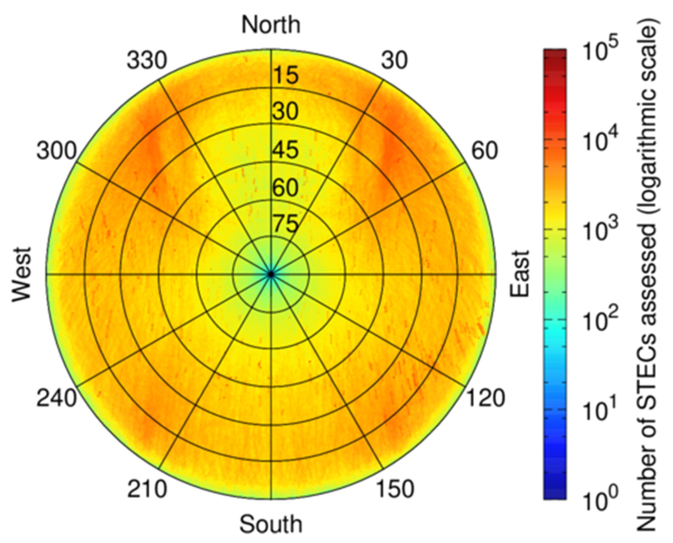
1st Dec	754	90	32	21	24	10	3	168042064

summarizes the number of STECs computed in the present study along 2019. They correspond to a total number of 2125 million STECs, 168 of which are VTECs. The processing involved up to 92 satellites tracked by up to 796 stations of the entire IGS MGEX network. In this manner, any possible combination of elevation and azimuth is thoroughly assessed with actual data measurements, actual station coordinates, and actual satellite orbits and clocks. Unlike [6], the extreme redundancy of stations allows addressing the vertical case, which uses a simplified algorithm with respect to the slant case (see Figure 10 in [6] for an overview of the hierarchy of the functions). In this sense, Figure 2 depicts a sky plot example for 1st of March 2019 accumulating the 190 million STECS from 796 stations and 92 satellites into a single image, as if they occurred at a unique location.

4.1. Analysis of Discrepancies

After processing such a large amount of data, only few discrepancies arise, which is a very positive outcome. Numerically, over 2125 million STECs are equal, which account for 99.998% of the total.

Table 2. Details of the comparison between ESA and JRC libraries implementations. For every day assessed within 2019, we count the total number of stations and STECs, specifying the number of equal STECs and the different STECs for the discrepancy types detailed in Section 4.1.

Date	STA	STECs	EQUAL STECs		DIFFERENT STECs
					Case 1		Case 2
	TOTAL	TOTAL	TOTAL	(%)	TOTAL	(%)	TOTAL	(%)
1st Jan	777	170746858	170744369	99.9985	0	0	2489	0.0015
1st Feb	785	186957831	186954954	99.9985	2	1.13 × 10−6	2877	0.0015
1st Mar	796	190740837	190738001	99.9985	0	0	2836	0.0015
1st Apr	795	176862405	176859745	99.9985	0	0	2658	0.0015
1st May	786	177651747	177648785	99.9983	0	0	2962	0.0017
1st Jun	791	177102278	177098998	99.9981	0	0	3280	0.0019
1st Jul	790	178653441	178650745	99.9985	0	0	2696	0.0015
1st Ago	793	180363367	180360010	99.9981	0	0	3357	0.0019
1st Sep	797	178434929	178430159	99.9973	0	0	4770	0.0027
1st Oct	782	176079189	176073057	99.9965	0	0	6132	0.0035
1st Nov	739	163914243	163910332	99.9976	0	0	3911	0.0024
1st Dec	754	168042064	168037938	99.9975	0	0	4126	0.0025
TOTAL		2125549189	2125507093	99.9980	2	1.13 × 107	42,094	0.00198

summarizes the discrepancies found on every day. Such discrepancies have been classified into two different types:

i.

Case 1: Both JRC and ESA software calculate a STEC value, but there is a numerical discrepancy.

ii.

Case 2: JRC software does not calculate a STEC value for that particular case, whereas ESA assigns a zero value.

Case 1: 2 STEC computed values are different for station "SIN1" on 1st April 2019. However, the discrepancy occurs at the fifth and last decimal place, hence, it is attributed to the rounding error and can be safely disregarded.

Case 2: For 42,094 STECs, which account for 0.0019% of the total, we found that the behavior of the two NeQuick-G implementations differs. These particular STECs correspond to satellite elevations less than 0.5 degrees. This result suggests that it is a limitation of the NeQuick-G model and not an error attributable to the implementations. According to [5], there is one specific case where the geometry between receiver and satellite is considered as invalid:

If invalid ray, i.e., |pdZeta| > 90.0 and pstRay →dR < Reset return value error to true

where pdZeta is the zenith angle of point 2 seen from point 1 (being point 1 and p2 the positions of satellite (p2) and receiver (p1), respectively), pstRay corresponds to the pointer ray, which is the straight line passing through p1 and p2, and dR stands for the range of the point from the center of the Earth.

Additionally, in fact, this would correspond to these particular cases. How do the different implementations deal with it? The JRC implementations do not return any STEC output, whereas the ESA implementation returns a null (i.e., zero) STEC value. The first option would be more aligned with the if-condition named “invalid ray” shown above, which has been foreseen in the official document [5]. In contrast, yielding a zero STEC can pose a large miss-modeling when the user computes its coordinates. Understanding these discrepancies is important when evaluating the ionospheric predictions of a 3D ionospheric model, which would be the case of NeQuick-G and the main goal of this manuscript. However, these particular differences are not critical for positioning purposes since the minimum elevation masks usually employed by Earth users range between 5 to 10 degrees.

In light of the divergence found for elevations less than 0.5 degrees, and brought to the attention of one of the reviewers, we have also considered the case where elevations become negative i.e., under a radio occultation (RO) scenario.

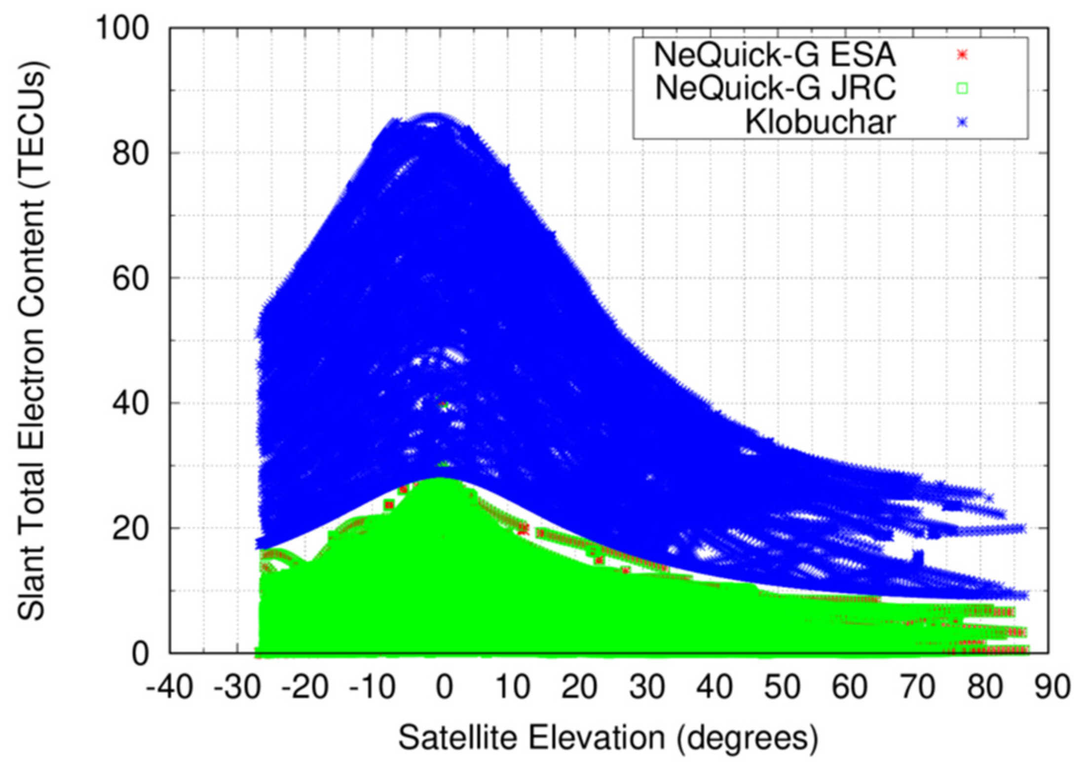
Case 3: In order to explore the behavior of the two NeQuick-G implementations for negative elevations, it has been needed to use data from a low Earth orbit (LEO) satellite since it is not possible to track a GNSS satellite with negative elevations from a GNSS station on ground. The selected RO mission is COSMIC-2 [28] and the processed DOY is 274 for year 2019 (i.e., 1st of October 2019). Results are shown in Figure 3, expressed in total electron content units (TECUs), where 1 TECU corresponds to 0.162 m of delay at the L1 frequency. To better interpret the results, the Klobuchar model has also been used to calculate STECs, although it is an ICA tuned for users close to the ground and hence, for LEO satellites clearly over-estimates the electron content between the on-board receiver and the GPS transmitter.

As one can deduct from Figure 3, NeQuick-G seems to be also capable of modeling STECs of RO conditions. That is, with negative satellite elevations down to few tens of degrees. The two implementations of ESA and JRC yield identical STECs, except for the discrepancy aforementioned in Case 2. The examined 24 h contains a total of 142,778 STECs, in which 24 rays at elevations comprised from −19° to −27° cannot be computed in the JRC implementation, whereas the ESA code outputs a zero STEC for those cases.

Although Figure 3 shows us that both ICAs are able to calculate STECs for negative elevations, the question posed is, how realistic are those outputs? The ground station EBRE was selected to compare the STECs computed using NeQuick-G and Klobuchar, respectively, against those of COSMIC-2. The reference values are the GF combination of carrier-phase measurements, having estimated their carrier-phase ambiguity $\langle B_{GF}\rangle$ with the CCL procedure. Figure 4 depicts that NeQuick-G largely underestimates the STECs from the LEO but reproduces quite well the STECs computed for a permanent receiver on ground. Therefore, at the light of these preliminary comparatives, NeQuick-G and Klobuchar seem not suitable for GNSS scenarios involving RO conditions (i.e., negative elevations).

4.2. Analysis of Execution Time

As mentioned, the UNIX utility “time” has been used in order to measure the time needed to execute each ICA in a racked computer Intel(R) Xeon(R) CPU E5-2650 0 @ 2.00 GHz. Although gLAB supports multithreading, for the purpose of this analysis, every gLAB process used one single-thread. All times presented will be referred to this particular computer.

In terms of execution time, initially, the ESA NeQuick-G code resulted in being 31% slower than that of JRC. In order to be fair with the inter-comparison, the ESA code was thoroughly reviewed in order to eliminate any superfluous and unnecessary instruction. By doing this, the execution time of ESA was significantly improved and the final results are going to be discussed as follows.

The NeQuick-G implementations took 808,407 s for ESA and 712,287 s for JRC, to complete the whole test benchmark (which corresponds to an average of 86.13 and 75.89 s of processing time per station, respectively). This implies that JRC implementation is 11.84% faster than the ESA one. In order to eliminate the overhead of using NeQuick-G as a library, we embedded the JRC implementation inside gLAB source code. The execution time reduced the results of the JRC library by 2.25%, down to 696,231 s (74.17 s per station), which corresponds to an improvement of 13.87% with respect to the ESA implementation in form of library. The reduction is mainly attributed to the fact that the 12 CCIRs and the MODIP are stored within the source code as variables at the compilation time, whereas when in the form of a library, they are accessed as external files. Finally, in order to complete our ICA assessment, the Klobuchar model also ran for the same whole test benchmark. The execution time was 154,869 s (16.5 s per station), reducing 77.76% (i.e., a factor 4.5) the time of the quickest NeQuick-G implementation of JRC.

As pointed out in the introduction, the execution time of NeQuick-G is a crucial point to take into account. Several initiatives have been already presented in order to reduce its computational burden (see for instance [13,29,30] in chronological order). More precisely, in [29], the ionospheric disturbance flags broadcast in the Galileo navigation message are used to control the tolerance and number of iterations in the iterative process within the TEC integration in the NeQuick-G algorithm. In [30], some optimizations were tested that range from changes in the model itself by storing pre-computed parameters in look-up-tables to changing the integration routine parameters. In [13], different integration methods were tested to try and reduce the computational burden of NeQuick-G, which is correlated to the number of calls inside the TEC calculation to the ionospheric model.

4.3. Analysis of the Memory Consumption

The study includes an analysis in terms of memory requirements for implementing the NeQuick-G ICA by request of one of the reviewers. Although memory resources are no longer a concern in modern desktop computers, it can be a limiting factor in some mass market segments such as embedded devices (i.e., smartphones or other handheld devices). In this regard, some initiatives have been already proposed to assess the compromise between the computational burden of NeQuick-G and its accuracy in smartphones [31].

Let us remember that NeQuick-G is a SW candidate to be integrated in low cost equipment with little random access memory (RAM) available and to be massively produced. RAM used by NeQuick-G ESA and JRC are by default the same. In practice: RAM memory required for both implementations is approximately 50 Kbytes. It is worth noticing that most of the memory consumption is required by the storage of CCIR and MODIP files. Provided these constants are assumed to be fixed and are stored in read only memory (ROM), the amount of RAM required can be reduced. In fact, this is an option available in the NeQuick-G implementation from the JRC termed “FTR_MODIP_CCIR_AS_CONSTANTS” that reduces the RAM usage to 13 Kbytes by not coping to the RAM the MODIP coefficients, nor the spherical harmonic coefficients from CCIR maps. For comparison purposes, we also examined the Klobuchar model, which uses a total of 184 bytes of memory, including the memory allocated for the 8 parameters broadcast in the GPS navigation message.

4.4. Analysis of the STEC Accuracy

Figure 5 depicts the results of the consistency test applied to the STEC computed by NeQuick-G (red) and Klobuchar (blue) aggregating the 12 days of 2019 used for the whole analysis. Recall that the residuals are computed with respect to IAR reference STEC values. We present the cumulative distribution function (CDF) of errors up to 10 TECUs in the top plot, where the NeQuick-G over performs Klobuchar. The bottom plot shows a zoom of the percentiles greater than 90%, in which we can observe how for errors greater than 12.15 TECUs (percentile 96.23th), the Klobuchar model produces STECs with lower errors. As already pointed out in the methodology section, the values on the tails of the error distributions influence the overall RMS value.

Table 3. Results of the consistency test between unambiguous and unbiased reference ionospheric values and the prediction computed by Galileo and GPS ICAs.

Metric	STEC Residuals (TECU)
	NeQuick	Klobuchar
Mode	0.07	0.08
Mean	3.32	4.04
50%	2.09	3.11
68%	3.35	4.62
95%	10.64	11.07
99%	20.72	17.87
99.9%	37.89	30.30
RMS	5.29	5.54

provides a more complete statistical description of the CDFs depicted in Figure 5 than merely the RMS, by summarizing some percentiles values numerically. It can be seen that for the lowest percentiles the NeQuick-G model reduces up to 49% the residual errors of Klobuchar. It can also be observed that for the 99% percentile and greater, the Klobuchar errors are smaller than those of NeQuick-G. This provides a greater insight to the model performance than the RMS, which only differs in 5%.

4.5. Analysis of the PVT Accuracy

Figure 6 presents the CDF of the 3D positioning errors obtained when using the NeQuick-G and Klobuchar models. In a similar manner than in the previous analysis, we depict the CDF for rather small PVT errors in the top panel and a zoom of the CDF values greater than 90% in the bottom panel. As commented in the methodology section, for every ICA, we performed the estimation of the PVT with code-only pseudorange measurements and with CCL measurements. In this regard, it can be seen how the CDF curves of NeQuick-G ICA improve those of Klobuchar, up to 5.76 m (percentile 99.18th) for code-pseudorange measurements and up to 4.98 m (percentile 98.29th) for CCL measurements. This reflects the contribution of the code pseudorange measurements to the PVT errors. The effect of the tails of the PVT error distribution can be observed in the bottom panel; PVT errors obtained with CCL measurements are smaller than those of code-pseudorange measurements up to at 4.18 m (percentile 97.13th) in NeQuick-G and 5.23 m (percentile 98.60th) in Klobuchar. The worsening of CCL with respect to code pseudorange is attributable to a smaller number of satellites used to compute the PVT solution, after the necessary cycle-slip detection for the CCL process. As we can see, this only affects the large percentiles of

Table 4. Percentile values of the PVT 3D positioning errors obtained with NeQuick-G and Klobuchar using code-pseudorange measurements and CCL measurements.

Metric	3D Positioning Error with C1P (m)		3D Positioning Error with CCL (m)
	NeQuick-G	Klobuchar	NeQuick-G	Klobuchar
Mode	0.93	1.12	0.58	1.21
Mean	1.47	1.97	1.26	1.83
50%	1.20	1.76	0.93	1.62
68%	1.61	2.30	1.29	2.05
95%	3.52	4.07	3.40	3.81
99%	5.50	5.56	5.90	5.73
99.9%	8.92	8.47	13.02	12.82
RMS	1.83	2.28	1.79	2.21

, and, in turn, the RMS values.

5. Conclusions

The authors conclude that both ESA and JRC implementations of NeQuick-G are suitable candidates to be integrated into gLAB, according to the results of the present extensive testing campaign involving over 2125 million STECs of permanent stations and a COSMIC-2 LEO satellite. Both have shown to be compliant with the official reference document and their robustness against real scenarios.

The final selection has been the JRC implementation embedded inside the gLAB source code (i.e., not called as an external library). The reasons that support our choice are: it does not yield a null STEC value when the geometry of the ray is considered to be bad following [5], it is 13.88% faster than the ESA implementation, and it is distributed with a EUPL license which allows a worldwide-unlimited distribution within gLAB.

Once the Galileo ICA has been integrated into gLAB, it is possible to compare it against the GPS ICA in terms of accuracy in the range domain and in the terms of accuracy in the position domain, which ultimately, is what gLAB users are interested in. NeQuick-G outperforms the Klobuchar model in the STEC residuals up to 12.15 TECUs (percentile 96.23th) and in the 3D position errors, up to 5.76 m (percentile 99.18th) for code-pseudorange positioning. Nevertheless, the performance gain of NeQuick-G should be balanced against the model complexity and execution time.